Toward the full short-time statistics of an active Brownian particle on the plane

Abstract

We study the position distribution of a single active Brownian particle (ABP) on the plane. We show that this distribution has a compact support, the boundary of which is an expanding circle. We focus on a short-time regime and employ the optimal fluctuation method (OFM) to study large deviations of the particle position coordinates $x$ and $y$. We determine the optimal paths of the ABP, conditioned on reaching specified values of $x$ and $y$, and the large deviation functions of the marginal distributions of $x$, and of $y$. These marginal distributions match continuously with “near tails” of the $x$ and $y$ distributions of typical fluctuations, studied earlier. We also calculate the large deviation function of the joint $x$ and $y$ distribution $P(x,y,t)$ in a vicinity of a special “zero-noise” point, and show that $\ln P(x,y,t)$ has a nontrivial self-similar structure as a function of $x$, $y$ and $t$. The joint distribution vanishes extremely fast at the expanding circle, exhibiting an essential singularity there. This singularity is inherited by the marginal $x$- and $y$-distributions. We argue that this fingerprint of the short-time dynamics remains there at all times.

I Introduction

Spatio-temporal dynamics of active self-propelled particles has been a subject of much current interest, both theoretically and experimentally. Contrary to passive Brownian particles, that are driven by thermal noise, generated via the collisions with molecules in a surrounding fluid, a self-propelled active particle consumes energy directly from the environment and moves ballistically in a stochastically evolving direction with an intrinsic velocity $v_{0}$. Such active particles occur in many biological and soft matter systems including E. coli bacteria, fish schools, colloidal surfers amongst others (for reviews, see e.g. Refs. Romanczuk ; soft ; BechingerRev ; Marchetti2017 ). Interaction between self-propelled particles leads to new phases and other interesting collective properties. Numerous recent studies have revealed that, even without interaction, just a single self-propelled particle displays interesting and complex spatio-temporal patterns that are yet to be fully understood. Three simple models of a single self-propelled particle have been studied extensively: active Brownian motion (ABM), run-and-tumble particle and active Ornstein-Uhlenbeck process. In this paper, we focus on the ABM only and study its position distribution in two dimensions at short times (or equivalently in the strongly-active limit) when the position distribution is highly anisotropic and non-Gaussian. We show that, at short times, the large deviation properties of the position distribution can be extracted analytically using the optimal fluctuation method.

The ABM in two dimensions is defined as follows. Let $(x(t),y(t))$ denote the position of the self-propelled particle at time $t$. There is an intrinsic velocity vector attached to the particle (like a “spin”) $\vec{v}=(v_{0}\,\cos\phi(t),v_{0}\,\sin\phi(t))$, where $\phi(t)$ denotes the angle of orientation of the spin vector at time $t$. The orientation angle $\phi(t)$ performs a rotational Brownian motion with diffusion constant $D$. We assume that there is no direct translational noise present. The three degrees of freedom $x$, $y$ and $\phi$ then evolve in time according to the equations

$$\dot{x} = v_{0}\cos\phi(t),$$ (1)

$$\dot{y} = v_{0}\sin\phi(t),$$ (2)

$$\dot{\phi} = \sqrt{2\,D}\,\eta(t)\,,$$ (3)

where $\eta(t)$ is a Gaussian white noise with zero mean and a correlator $\langle\eta(t)\eta(t^{\prime})\rangle=\delta(t-t^{\prime})$. We assume that the particle starts from the origin, $x(0)=0$ and $y(0)=0$, with an initial orientation angle $\phi(0)$. The most basic question in this problem concerns the position distribution $P(x,y,t)$ of the particle in the $xy$ plane at time $t$ BechingerRev ; Marchetti2017 ; Solon2015 ; GPB2015 ; Seifert ; Franosch ; Basu2018 ; GL2018 ; Basu2019 ; SDC2020 .

To establish some basic properties of the distribution $P(x,y,t)$, let us first integrate (1) and (2) up to time $t$ starting from the origin

$$x(t) = v_{0}\,\int_{0}^{t}\cos\phi(t^{\prime})\,dt^{\prime}\,,$$ (4)

$$y(t) = v_{0}\,\int_{0}^{t}\sin\phi(t^{\prime})\,dt^{\prime}\,.$$ (5)

Taking squares of Eqs. (4) and (5) and adding the two equations, we obtain, for arbitrary $t\geq 0$:

$$x^{2}(t)+y^{2}(t) = v_{0}^{2}\,\int_{0}^{t}\int_{0}^{t}\cos\left[\phi(t_{1})-\phi(t_{2})\right]\,dt_{1}\,dt_{2}$$ (6)

$$\leq v_{0}^{2}\,t^{2}\,.$$

That is, the particle cannot be found beyond the expanding circle of radius $v_{0}t$, as to be expected on physical grounds. Moreover, the equality in Eq. (6) is satisfied if and only if $\phi(t_{1})=\phi(t_{2})$ for all $t_{1}$ and $t_{2}$ in the time interval $[0,t]$, i.e., if $\phi(t^{\prime})=\phi(0)$ for all $t^{\prime}\in[0,t]$. Therefore, the equality $x^{2}(t)+y^{2}(t)=v_{0}^{2}\,t^{2}$ holds only at the zero-noise point $(v_{0}\,t\,\cos\phi(0),v_{0}\,t\,\sin\phi(0))$ on the circumference of the circle of radius $v_{0}t$. At any other point on the circumference, the strict inequality holds: again, as to be expected. That is, the distribution $P(x,y,t)$ must be supported over the circle of radius $v_{0}\,t$ and, moreover, it must strictly vanish at all points on the circumference of the circle except at $(v_{0}\,t\,\cos\phi(0),v_{0}\,t\,\sin\phi(0))$. However, calculating $P(x,y,t)$ inside this circle is a challenging problem.

In fact, the ABM model was originally introduced in the mathematics literature, as the ‘random curvature’ model, by Mumford Mumford . He studied random algebraic curves in two dimensions in the context of computer vision, much before the ABM re-surfaced in the literature on active systems. The position distribution $P(x,y,t)$ can, in principle, be obtained by integrating out the orientational degree of freedom from the full probability density, $P(x,y,t)=\int P(x,y,\phi,t)\,d\phi$, where $P(x,y,\phi,t)$ satisfies the Fokker-Planck equation

$$\frac{\partial}{\partial t}P(x,y,\phi,t)=-v_{0}\left(\cos\phi\frac{\partial P}{\partial x}+\sin\phi\frac{\partial P}{\partial y}\right)+D\,\frac{\partial^{2}P}{\partial\phi^{2}}$$ (7)

with the initial condition,

$$P(x,y,\phi,t=0)=\delta(x)\,\delta(y)\,\delta(\phi-\phi(0))\,.$$

However, solving this Fokker-Planck equation and extracting $P(x,y,t)$ explicitly is hard (to quote Mumford, “I have looked for an explicit formula for $P$ but in vain” Mumford ). When averaged over the initial orientation $\phi(0)$ distributed uniformly in $[0,2\pi]$ (that makes $P(x,y,t)$ isotropic at all times), it is possible to write a formal expression for the Fourier transform $f(k,t)=\langle e^{i\vec{k}\cdot\vec{r}(t)}\rangle$ in terms of the eigenfunctions of Mathieu operator Franosch . Nevertheless, to explicitly extract from this formal expression the position distribution $P(x,y,t)$ in the real space is not easy.

The origin of the difficulty in the deceptively simple process (1)-(3) is in the nonlinearity of the functions $\cos\phi$ and $\sin\phi$, leading to a strongly non-Gaussian character of the orientationally driven noises acting on $x$ and $y$. Moreover, writing $\dot{x}=v_{0}\,\cos\phi(t)=\xi_{x}(t)$ and $\dot{y}=v_{0}\,\sin\phi(t)=\xi_{y}(t)$, we see that the noises $\xi_{x}(t)$ and $\xi_{y}(t)$ are both correlated in time. Using the Brownian properties of $\phi(t)$, the two-time correlation function of $\xi_{x}(t)$ can be easily computed  Basu2018

$$\langle\xi_{x}(t_{1})\xi_{x}(t_{2})\rangle\simeq\frac{v_{0}^{2}}{2}\exp\left[-D\,|t_{1}-t_{2}|\right]\,,$$ (8)

for large $t_{1}$ and $t_{2}$ with $|t_{1}-t_{2}|$ fixed, and similarly for $\xi_{y}(t)$. Thus, for short times, $t\ll D^{-1}$, the noise $\xi_{x}(t)$ is strongly correlated in time (as opposed to passive Brownian motion where the noise is delta-correlated). This makes the process non-Markovian and hence more difficult to analyse. The short-time limit $t\ll D^{-1}$ is called the strongly active limit.

In contrast, for $t\gg D^{-1}$, the noise correlator converges to $\langle\xi_{x}(t_{1})\xi_{x}(t_{2})\rangle\to 2\,D_{\text{eff}}\,\delta(t_{1}-t_{2})$ with an effective diffusion constant $D_{\text{eff}}=v_{0}^{2}/(2D_{R})$. Thus, in this strongly passive limit $t\gg D^{-1}$, the ABM effectively reduces to an ordinary $2$-d Brownian motion, and the position distribution, irrespective of the initial orientation $\phi(0)$, converges to an isotropic Gaussian form

$$P(x,y,t)\simeq\frac{1}{4\,D_{\rm eff}\,t}\,\exp\left[-\frac{(x^{2}+y^{2})}{4\,D_{\rm eff}\,t}\right]\,,$$ (9)

which holds for typical fluctuations, i.e., when $x\sim\sqrt{t}$ and $y\sim\sqrt{t}$. For large atypical fluctuations, when $r=\sqrt{x^{2}+y^{2}}\sim v_{0}\,t$, the position distribution is described by the large deviation form

$$P(x,y,t)\sim\exp{\left[-tD_{R}\,\Psi\left(\frac{\sqrt{x^{2}+y^{2}}}{v_{0}\,t}\right)\right]}\,,$$ (10)

where the rate function $\Psi(z)$ was recently computed analytically Basu2019 .

It was pointed out in Ref. Basu2018 that in the strongly active short-time regime $t\ll D^{-1}$, the position distribution at time $t$ remembers the initial orientation $\phi(0)$ and is strongly anisotropic and non-Gaussian, which are fingerprints of ‘activity’ that gets washed out at late times when $t\gg D^{-1}$. For a fixed initial orientation, say $\phi(0)=0$, it was shown in Ref Basu2018 that $P(x,y,t)$, at $t\ll D^{-1}$, is peaked at $(x=v_{0}\,t,y=0)$ with typical fluctuations of $x$ and $y$ scaling as $v_{0}\,t-x\sim t^{2}$ and $y\sim t^{3/2}$. The position distribution, in this typical regime, is described by the scaling form Basu2018

$$P(x,y,t)\simeq\frac{1}{\sqrt{2}\,v_{0}^{2}\,D^{3/2}\,t^{7/2}}\,{\tilde{P}}\left(\frac{v_{0}t-x}{v_{0}\,D\,t^{2}},\frac{y}{v_{0}\,\sqrt{2\,D}\,t^{3/2}}\right)\,,$$ (11)

where the double Laplace transform of the scaling function ${\tilde{P}}(a_{1},a_{2})$ was computed exactly Basu2018 . Inverting explicitly this Laplace transform to extract $P(x,y,t)$ in the typical regime of $x$ and $y$ is difficult and has not been performed up to now. In contrast, the marginal distributions $p_{x}(x,t)=\int dy\,P(x,y,t)$ and $p_{y}(y,t)=\int dx\,P(x,y,t)$ were explicitly computed in the typical fluctuation regime, leading to the expressions

$$p_{x}(x,t) = \frac{1}{v_{0}\,D\,t^{2}}\,f_{x}\left(\frac{v_{0}\,t-x}{v_{0}\,D\,t^{2}}\right)\,,$$ (12)

$$p_{y}(y,t) = \frac{1}{v_{0}\,\sqrt{2D},t^{3/2}}\,f_{y}\left(\frac{y}{v_{0}\,\sqrt{2D}\,t^{3/2}}\right)\,,$$ (13)

The scaling function $f_{x}(z)$, supported over $z\in[0,\infty]$, is highly non-Gaussian and has the asymptotic tails Basu2018

$$f_{x}(z)\simeq\begin{cases}&\frac{1}{2\,\sqrt{\pi\,z^{3}}}\,e^{-1/(8\,z)}\quad{\rm as}\quad z\to 0\,,\\ \\ &\frac{1}{\sqrt{2\,z}}\,e^{-\pi^{2}\,z/8}\quad{\rm as}\quad z\to\infty\,.\end{cases}$$ (14)

In contrast, the scaling function for the $y$ marginal is a pure Gaussian Basu2018

$$f_{y}(z)=\sqrt{\frac{3}{2\,\pi}}\,e^{-3z^{2}/2}\,,\quad z\in[-\infty,\infty]\,.$$ (15)

However, the tails of the marginal distributions $p_{x}(x,t)$, $p_{y}(y,t)$, and the joint distribution $P(x,y,t)$ that characterize the atypical fluctuations of the positions $x$ and $y$, on a scale $x\sim v_{0}\,t$ and $y\sim v_{0}\,t$ at short times $t\ll D^{-1}$, are yet to be understood.

In this paper, we derive these large deviation tails by using the optimal fluctuation method. Our main results can be summarized as follows. For the marginal distributions we show that

$$-\ln p_{x}(x,t) \simeq \frac{1}{2Dt}\,s_{X}\left(X=\frac{x}{v_{0}\,t}\right)\,,$$ (16)

$$-\ln p_{y}(y,t) \simeq \frac{1}{2Dt}\,s_{Y}\left(Y=\frac{y}{v_{0}\,t}\right)\,,$$ (17)

where the two rate functions $s_{X}(X)$ and $s_{Y}(Y)$ are computed analytically in Eqs. (38) and (39), and Eqs. (49) and (50), respectively. We show that when $X\ll 1$ and $Y\ll 1$, these large deviation tails match smoothly with the typical behaviors in Eq. (12) and (13), respectively. At the edges of their supports, $x=-v_{0}t$ and $y=\pm v_{0}t$, respectively, the marginal distributions vanish extremely rapidly and exhibit essential singularities, see Eqs. (41) and (53). Equations (16) and (17) are asymptotically exact in the limit of $Dt\to 0$.

The joint distribution $P(x,y,t)$ exhibits the large deviation form

$$-\ln P(x,y,t)=\frac{1}{2Dt}\,s\left(X=\frac{x}{v_{0}\,t},Y=\frac{y}{v_{0}\,t}\right)\,.$$ (18)

In a close vicinity of the point $(X=1,Y=0)$ where the joint distribution has its maximum, we show that the rate function $s(X,Y)$ has an interesting self-similar structure:

$$s(X,Y)\simeq(1-X)\,F\left(\frac{1-X}{Y^{2}}\right)\,,$$ (19)

which follows from invariance of the governing equations in this limit under a stretching transformation. We computed the scaling function $F(z)$ analytically, see Eq. (82), and plotted it in Fig. 6. Similarly to the marginal distributions, this large deviation tail matches smoothly with the typical behavior of the joint distribution. Close to the point $(X=1,Y=0)$ Eqs. (18) and (19) become asymptotically exact in the limits of $Dt\to 0$, $1-X\to 0$ and $Y\to 0$ while keeping the ratio $z=(1-X)/Y^{2}$ constant.

The rest of the paper is organized as follows. In Section II we briefly introduce the optimal fluctuation method (OFM) and formulate the OFM problem for the position statistics of the ABP. The complete marginal distributions are calculated in Section III. In Section IV we study the joint distribution. Section V contains a brief summary and discussion. Some technical details are relegated to the three appendices.

II The short-time position statistics and the OFM

We consider the ABM model in two dimensions, defined in Eqs. (1)-(3), with the initial conditions $x(0)=y(0)=0$ and $\phi(0)=0$. Let us first establish some general facts. Purely on dimensional ground, the joint distribution $P(x,y,t)$, for arbitrary $t$, can be written as

$$P(x,y,t)=\frac{1}{v_{0}^{2}t^{2}}\,\Phi\left(X,Y,Dt\right),$$ (20)

where $X=x/(v_{0}t)$ and $Y=y/(v_{0}t)$ are the rescaled coordinates, and

$$\int_{-\infty}^{\infty}\int_{-\infty}^{\infty}dX\,dY\Phi(X,Y,\,D\,t)=1.$$ (21)

In their turn, the exact marginal $x$- and $y$-distributions scale as

$$p_{x}(x,t)=\int_{-\infty}^{\infty}P(x,y,t)dy=\frac{1}{v_{0}t}\,f\left(X,Dt\right),$$ (22)

and

$$p_{y}(y,t)=\int_{-\infty}^{\infty}P(x,y,t)dx=\frac{1}{v_{0}t}\,g\left(Y,Dt\right),$$ (23)

where

$$f(X,Dt) = \int_{-\infty}^{\infty}\Phi(X,Y,Dt)\,dY,$$ (24)

$$g(Y,Dt) = \int_{-\infty}^{-\infty}\Phi(X,Y,Dt)\,dX.$$ (25)

As argued in the introduction, the exact distribution $P(x,y,t)$ vanishes outside the circle of unit radius $X^{2}+Y^{2}=1$. Consequently, the marginal $x$ and $y$ distributions live on the intervals $|X|\leq 1$ and $|Y|\leq 1$, respectively.

Here we will study the short-time behavior, $Dt\ll 1$, of $p_{x}(x,t)$, $p_{y}(y,t)$ and $P(x,y,t)$. Since we are interested in the large deviation regime $X\sim O(1)$ and $Y\sim O(1)$, we can employ the OFM.

II.1 Optimal fluctuation method

At short times we can calculate $P(x,y,t)$ up to a preexponential factor by applying the OFM which, for the Brownian motion, becomes geometrical optics  GF2003 ; Meerson2019 ; SmithMeerson2019 ; MeersonSmith2019 ; Agranovetal2020 ; MM2020 . The OFM boils down to a minimization of the action $S$ of the Brownian motion of the angle $\phi(t^{\prime})$,

$$-\ln P(x,y,t)\simeq S=\frac{1}{4D}\int_{0}^{t}{\dot{\phi}}^{2}(t^{\prime})\,dt^{\prime},$$ (26)

over all paths $\phi(t^{\prime})$ subject to the integral constraints

$$v_{0}\int_{0}^{t}\cos\phi(t^{\prime})dt^{\prime}=x\,,\quad v_{0}\int_{0}^{t}\sin\phi(t^{\prime})dt^{\prime}=y.$$ (27)

The boundary conditions for $\phi(t^{\prime})$, for $0\leq t^{\prime}\leq t$, are

$$\phi(t^{\prime}=0)=0\quad\text{and}\quad\dot{\phi}(t^{\prime}=t)=0,$$ (28)

where the second condition is the free-end boundary condition of the calculus of variations Elsgolts . Going over to the rescaled variables $X=x/(v_{0}t)$, $Y=y/(v_{0}t)$ and ${\tau}=t^{\prime}/t$, we immediately arrive at the OFM scaling behavior, announced in Eq. (18) [compare it with the exact scaling in (20)]. The rescaled OFM action

$$s(X,Y)=\frac{1}{2}\int_{0}^{1}{\dot{\phi}}^{2}(\tau)\,d\tau$$ (29)

plays the role of a rate function. The rescaled integral conditions (27) become

$$\int_{0}^{1}\cos\phi(\tau)d\tau=X$$ (30)

and

$$\int_{0}^{1}\sin\phi(\tau)d\tau=Y\,.$$ (31)

The two boundary conditions in (28) become

$$\phi(\tau=0)=0\quad\text{and}\quad\dot{\phi}(\tau=1)=0\,.$$ (32)

III Marginal distributions

We first study the short-time behavior of the marginal distributions $p_{x}(x,t)$ and $p_{y}(y,t)$.

III.1 Marginal distribution $p_{x}(x,t)$

Within the OFM framework, the marginal $x$-distribution has the form (16), where the rescaled action $s_{X}(X)$ should be evaluated by accounting only for the constraint (30). Introducing a Lagrange multiplier $\lambda$ to enforce this constraint, we can write the effective action as

$$s_{X}(X)=\frac{1}{2}\int_{0}^{1}{\dot{\phi}}^{2}(\tau)\,d\tau-\lambda\left(X-\int_{0}^{1}\cos\phi(\tau)\,d\tau\right)\,.$$ (33)

This action corresponds to the Lagrangian of a Newtonian particle in an effective potential $V(\phi)=-\lambda\,\cos\phi$. The Euler-Lagrange equation reads

$$\ddot{\phi}+\frac{\partial V}{\partial\phi}=\ddot{\phi}+\lambda\sin\phi=0\,.$$ (34)

This is the pendulum equation. Its energy integral is

$$\frac{\dot{\phi}^{2}}{2}-\lambda\cos\phi=E=\text{const}\,.$$ (35)

In view of the boundary conditions (32), the pendulum must start at $\tau=0$ from $\phi=0$ and stop at $\tau=1$. The least-action solution (the optimal path) is such that $\phi(\tau)$ is a monotonic function on the interval $0<\tau<1$, and we can choose it to be monotone increasing footnote1 . Therefore, (35) yields

$$\int_{0}^{\phi(\tau)}\frac{dz}{\sqrt{2\lambda(a+\cos z)}}=\tau.$$ (36)

Here we have already accounted for the condition $\phi(0)=0$ and introduced the parameter $a=E/\lambda$, so that $|a|<1$. The stopping point of the pendulum at $\tau=1$ is at $\phi(\tau=1)\equiv\phi_{*}=\arccos(-a)$, and $0<\phi_{*}<\pi$. Setting $\tau=1$ in (36), we obtain a relation between $\lambda$ and $a$:

$$\sqrt{2\lambda}=\int_{0}^{\phi_{*}}\frac{dz}{\sqrt{a+\cos z}}=\frac{2}{\sqrt{a+1}}\,F\left(\frac{\phi_{*}}{2},\frac{2}{a+1}\right),$$ (37)

where $F(\phi,m)=\int_{0}^{\phi}(1-m\sin^{2}z)^{-1/2}dz$ is the elliptic integral of the first kind. The constraint (30) yields a relation between $a$ and $X$:

$$X=\int_{0}^{1}\cos\phi(\tau)\,d\tau=\int_{0}^{\phi_{*}}\!\!\!\cos\phi\,\frac{d\tau}{d\phi}\,d\phi$$

$$=\int_{0}^{\phi_{*}}\!\!\frac{\cos z\,dz}{\sqrt{2\lambda\,(a+\cos z)}}\!=\!\frac{(a+1)E\left(\frac{\phi_{*}}{2},\frac{2}{a+1}\right)}{F\left(\frac{\phi_{*}}{2},\frac{2}{a+1}\right)}-a,$$ (38)

where $E(\phi,m)=\int_{0}^{\phi}(1-m\sin^{2}z)^{1/2}\,dz$ is the elliptic integral of the second kind, and we have used (37). Now we can express the action $s$ in (33) via $a$. Using the energy integral (35), we obtain

$$s_{X}(a) = {\lambda}\int_{0}^{1}\left(a+\cos\phi\right)\,d\tau={\lambda}\,(a+X)$$ (39)

$$= 2\,F\left(\frac{\phi_{*}}{2},\frac{2}{a+1}\right)\,E\left(\frac{\phi_{*}}{2},\frac{2}{a+1}\right),$$

where we have used Eqs. (30), (37) and (38).

Equations (38) and (39) determine the action $s=s_{X}(X)$ in the parametric form $X=X(a),\;s=s_{X}(a)$. A plot of $s=s_{X}(X)$ is shown in Fig. 1. Also shown are two asymptotes of $s_{X}(X)$, for $1-X\ll 1$ and for $1+X\ll 1$:

$$s_{X}(X)\simeq\begin{cases}&\frac{\pi^{2}}{4}\left(1-X\right),\quad\quad 1-X\ll 1,\\ \\ &\frac{4}{1+X},\quad\quad\quad\quad\quad 1+X\ll 1.\end{cases}$$ (40)

The upper line in (40) correspond to $1+a\ll 1$, the lower line to $1-a\ll 1$.

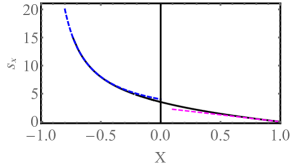
Figure 1: Solid line: the rescaled action $s_{X}(X)$, given by Eqs. (38) and (39). The dashed lines are the asympto- tics (40).

Equation (16) with the OFM rate function, defined parametrically by Eqs. (38) and (39), gives a complete description of large deviations of $x$. The asymptotic $1-X\ll 1$ from (40) describes an exponential tail of $p_{x}(x,t)$,

$$-\ln p_{x}(x,t)\simeq\frac{\pi^{2}(v_{0}t-x)}{8Dv_{0}t^{2}},\quad Dv_{0}t^{2}\ll v_{0}t-x\ll v_{0}t.$$ (41)

The left strong inequality guarantees that the action (26) is large, $S\gg 1$, as required for the applicability of the OFM. The “near tail” (41) agrees with the tail of of the typical behavior of $p_{x}(x,t)$ in the second line of Eq. (14).

The asymptotic $1+X\ll 1$ in (40) describes an essential singularity of the marginal distribution $p_{x}(x,t)$ at the leftmost point of its support, $x=-v_{0}t$, where the distribution vanishes, together with all its $x$-derivatives, extremely fast:

$$-\ln p_{x}(x\to-v_{0}t,t)\simeq\frac{2v_{0}}{D(v_{0}t+x)}.$$ (42)

III.2 Marginal distribution $p_{y}(y,t)$

In this case the OFM ansatz takes the form Of Eq. (17), where the rescaled action $s_{Y}(Y)$ should be evaluated by accounting only for the constraint (31). Introducing a proper Lagrange multiplier $\lambda$, we can write the effective rescaled action as

$$s_{Y}(Y)=\frac{1}{2}\int_{0}^{1}{\dot{\phi}}^{2}(\tau)\,d\tau+\lambda\left(Y-\int_{0}^{1}\sin\phi(\tau)\,d\tau\right)\,.$$ (43)

This is the Lagrangian of a Newtonian particle in an effective potential $V(\phi)=\lambda\,\sin\phi$. The Euler-Lagrange equation reads

$$\ddot{\phi}+\frac{\partial V}{\partial\phi}=\ddot{\phi}+\lambda\cos\phi=0,$$ (44)

with the energy integral

$$\frac{\dot{\phi}^{2}}{2}+\lambda\,\sin\phi=E\,.$$ (45)

As the $y$-distribution is symmetric with respect to $y=0$, it suffices to consider $y>0$. Here $\phi(\tau)$ increases monotonically from $\phi=0$ until the pendulum stops at $\tau=1$. The calculations are similar to those for the $p_{x}(x,t)$. We define, as before, $a=E/{\lambda}$ (note that $|a|<1$) and integrate Eq. (45), using the boundary conditions $\phi(\tau=0)=0$ and ${\dot{\phi}}(\tau=1)=0$. This gives

$$\sqrt{2\lambda}=\int_{0}^{\phi(1)}\frac{d\phi}{\sqrt{a-\sin\phi}}\,,$$ (46)

where $\sin\phi(1)=a$. Defining $\phi_{*}=\arccos(-a)$, we obtain $\phi(1)=\phi_{*}-\pi/2$. Making a change of variable $\phi=z-\pi/2$, one can express the integral in Eq. (46) in terms of the elliptic function $F(\phi,m)$, defined earlier. We obtain

$$\sqrt{2\lambda}=\frac{2}{\sqrt{a+1}}\,\left[F\left(\frac{\phi_{*}}{2},\frac{2}{a+1}\right)-F\left(\frac{\pi}{4},\frac{2}{a+1}\right)\right]\,.$$ (47)

Using Eq. (45), we express the constraint (31) as

$$Y = \int_{0}^{1}\sin\phi(\tau)\,d\tau=\int_{0}^{\phi(1)}\sin\phi(\tau)\,\frac{d\tau}{d\phi}\,d\phi$$ (48)

$$= \frac{1}{\sqrt{2\lambda}}\,\int_{0}^{\phi(1)}\frac{\sin\phi\,d\phi}{\sqrt{a-\sin\phi}}$$

$$= \frac{1}{\sqrt{2\lambda}}\left[a-\int_{0}^{\phi(1)}\sqrt{a-\sin\phi}\,d\phi\right]\,,$$

where we used the identity $\sin\phi=a-(a-\sin\phi)$ in arriving at the third line from the second line. Making the same change of variable $\phi=z-\pi/2$, we can express the integral in terms of the elliptic function $E(\phi,m)$. Finally, eliminating $\sqrt{2\lambda}$ from Eqs. (48) and (47), we obtain

$$Y=a-(a+1)\,\frac{E\left(\frac{\phi_{*}}{2},\frac{2}{a+1}\right)-E\left(\frac{\pi}{4},\frac{2}{a+1}\right)}{F\left(\frac{\phi_{*}}{2},\frac{2}{a+1}\right)-F\left(\frac{\pi}{4},\frac{2}{a+1}\right)}\,.$$ (49)

The action $s$ in (43) can also be evaluated:

$$s_{Y}(a) = \lambda(a-Y)$$ (50)

$$= 2\,\left[F\left(\frac{\phi_{*}}{2},\frac{2}{a+1}\right)-F\left(\frac{\pi}{4},\frac{2}{a+1}\right)\right]$$

$$\times \left[E\left(\frac{\phi_{*}}{2},\frac{2}{a+1}\right)-E\left(\frac{\pi}{4},\frac{2}{a+1}\right)\right]\,,$$

where we used Eq. (47) for $\lambda$ and Eq. (49) for $Y$. Again, we obtained $s_{Y}(Y)$ in a parametric form, determined by Eqs. (49) and (50). A plot of $s_{Y}(Y)$ vs. $Y$, is shown in Fig. 2. One can also derive the following asymptotic behaviors of $s_{Y}(Y)$ for $|Y|\ll 1$ and $1-Y\ll 1$:

$$s_{Y}(Y)\simeq\begin{cases}&(3/2)Y^{2},\quad\quad\quad\quad\quad\quad|Y|\ll 1,\\ \\ &\frac{2(3-2\sqrt{2})}{1-|Y|},\quad\quad\quad\quad\quad 1-|Y|\ll 1.\end{cases}$$ (51)

These two asymptotics are also plotted in Fig. 2.

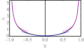
Figure 2: Solid line: the rescaled action $s_{Y}(Y)$, given by Eqs. (38) and (39). The dashed lines are asymptotics (51).

Using the asymptotic behavior (51) for $|Y|\ll 1$ in Eq. (17), and normalizing to unity, we obtain a Gaussian distribution which describes typical fluctuations of $y$, that is small distances, $|y|\ll v_{0}t$:

$$p_{y}(y,t)\simeq\frac{1}{\sqrt{2\pi\sigma_{y}^{2}}}\,e^{-\frac{y^{2}}{2\sigma_{y}^{2}}},\quad\text{where}\quad\sigma_{y}^{2}=\frac{2}{3}v_{0}^{2}Dt^{3},$$ (52)

This distribution is in perfect agreement with the typical behavior in (15). The complete $y$-distribution, however, is strongly non-Gaussian, as one can see from Eq. (50). In particular, it vanishes extremely rapidly at the leftmost and rightmost points of its support, $y=\pm v_{0}t$:

$$-\ln p_{y}(|y|\to v_{0}t,t)\simeq\frac{(3-2\sqrt{2})v_{0}}{D(v_{0}t-|y|)},$$ (53)

and has an essential singularity there, which is similar to that of the $x$-distribution at $x=v_{0}t$, see Eq. (42).

IV Joint distribution $P(x,y,t)$

Now we consider the joint distribution $P(x,y,t)$ in the $(X,Y)$ plane where $X=x/(v_{0}t)$ and $Y=x/(v_{0}t)$ are the rescaled co-ordinates. As we showed in the Introduction, the joint distribution is supported on the circle $X^{2}+Y^{2}=1$ of unit radius. For the initial condition $\phi(0)=0$, the distribution is peaked at $(X=1,Y=0)$ and vanishes at all other points on the circumference of the circle. At short times $P(x,y,t)$ obeys the OFM scaling behavior (18), and the rescaled action $s(X,Y)$ can be written as

$$s(X,Y) = \frac{1}{2}\int_{0}^{1}{\dot{\phi}}^{2}(\tau)\,d\tau-\lambda_{1}\,\left(X-\int_{0}^{1}\cos\phi(\tau)\,d\tau\right)$$ (54)

$$+ \lambda_{2}\,\left(Y-\int_{0}^{1}\sin\phi(\tau)\,d\tau\right)\,.$$

The two Lagrange multipliers $\lambda_{1}$ and $\lambda_{2}$ enforce the two constraints in Eqs. (30) and (31), respectively. In principle, one can determine the complete joint distribution in this formalism. This would require solving the effective mechanical problem, defined by the action (54), exactly. The exact solution can be obtained in elliptic functions. In this paper, however, we restrict ourselves for simplicity to a close vicinity of the point $(X=1,Y=0)$ where the probability density is the largest. Near this point we can use a small-angle approximation, which considerably simplifies the OFM analysis.

Indeed, when $X$ is very close to $1$, and $Y$ is small, it is clear from Eqs. (30) and (31), that $\phi(\tau)$ stays close to $0$ for all $0\leq\tau\leq 1$. This justifies the small-angle approximation, $\cos\phi\simeq 1-\phi^{2}/2$ and $\sin\phi\simeq\phi$. In this approximation the rescaled OFM action in (54) becomes

$$s(X,Y) \simeq \frac{1}{2}\int_{0}^{1}{\dot{\phi}}^{2}(\tau)\,d\tau-\lambda_{1}\left(X-1+\frac{1}{2}\int_{0}^{1}\phi^{2}(\tau)\,d\tau\right)$$ (55)

$$+ \lambda_{2}\left(Y-\int_{0}^{1}\phi(\tau)\,d\tau\right)$$

subject to the constraints

$$X = 1-\frac{1}{2}\int_{0}^{1}\phi^{2}(\tau)\,d\tau\,,$$ (56)

$$Y = \int_{0}^{1}\phi(\tau)\,d\tau\,.$$ (57)

The approximate effective action $s(X,Y)$ in Eq. (55) corresponds to the Lagrangian of a Newtonian particle in a parabolic potential

$$V(\phi)=\frac{\lambda_{1}}{2}\,\phi^{2}+\lambda_{2}\,\phi\,.$$ (58)

The Euler-Lagrange equation for the optimal path $\phi(t)$ reads

$$\ddot{\phi}=-\frac{\partial V(\phi)}{\partial\phi}=-\lambda_{1}\,\phi-\lambda_{2}=-\lambda_{1}(\phi+B)\,,$$ (59)

where $B=\lambda_{2}/\lambda_{1}$. The solution is elementary, but with a twist: It turns out that there are two branches of the solution, depending on the sign of $\lambda_{1}$. Let us consider the two cases separately.

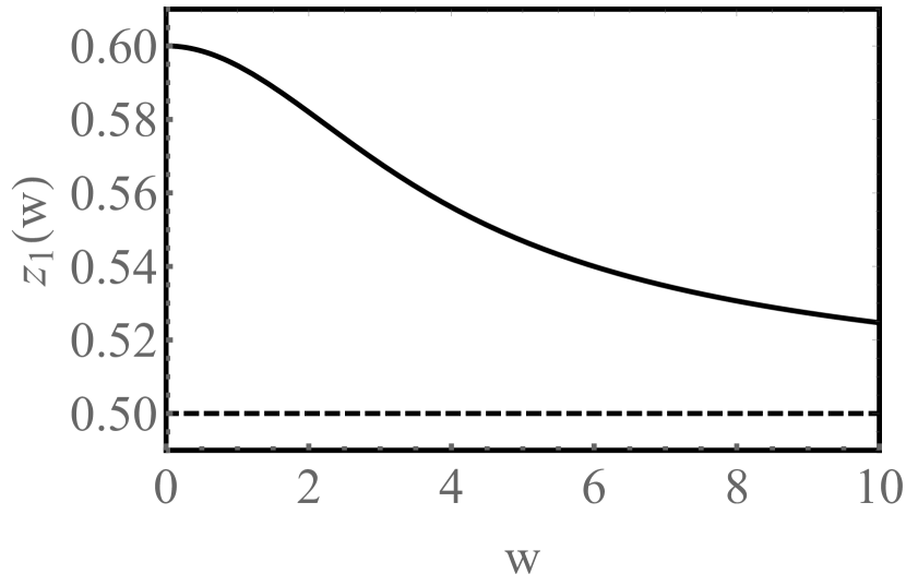
(a)

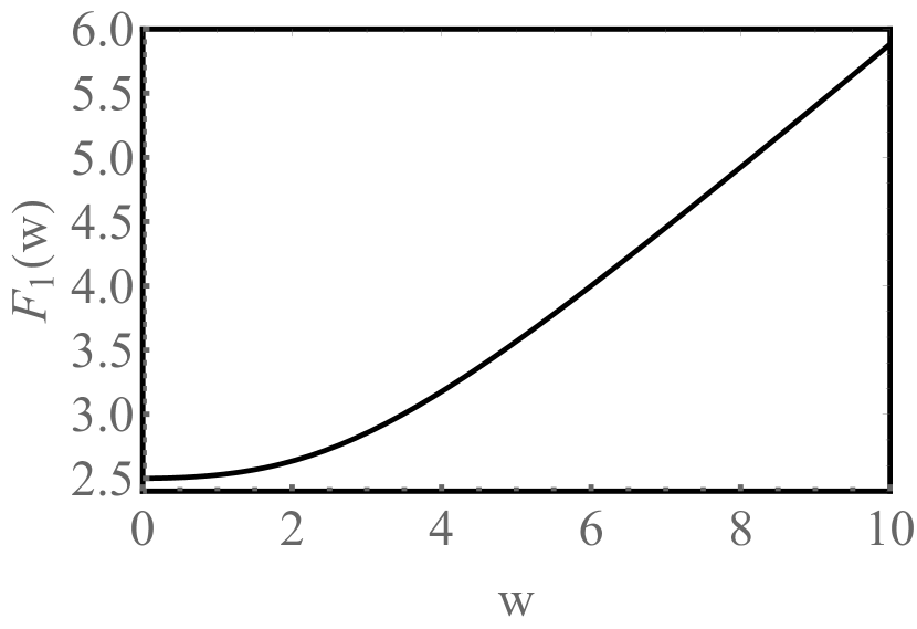
(b)

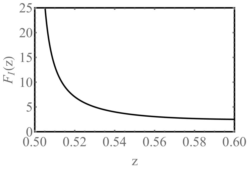
(c)

Figure 3: (a) The function $z_{1}(w)$ vs. $w$ from (67). As $w$ increases, $z_{1}(w)$ decreases monotonically from $z_{1}(0)=3/5$ and approaches $z_{1}=1/2$ as $w\to\infty$. (b) The function $F_{1}(w)$ vs. $w$ from (68). It increases monotonically with $w$ starting from $F_{1}(0)=5/2$. Asymptotically, $F_{1}(w)\to w/2$ as $w\to\infty$. (c) The scaling function $F_{\rm I}(z)$ vs. $z$, defined for $1/2\leq z\leq 3/5$ and determined parametrically by Eqs.  (77) and (76). When $z\to 3/5$, $F_{\rm I}(z)\to 5/2$, while for $z\to 1/2$, $F_{\rm I}(z)$ diverges as $[8\,(z-1/2)]^{-1}$.

IV.0.1 $\lambda_{1}\leq 0$: Branch I

For $\lambda_{1}\leq 0$ the particle moves in an inverted parabolic potential. Let us set $\lambda_{1}=-w^{2}$ with $w\geq 0$. Solving Eq. (59) with the boundary conditions $\phi(\tau=0)=0$ and ${\dot{\phi}}(\tau=1)=0$, we obtain

$$\phi(\tau)=B\,\left[\frac{\cosh\left(w(\tau-1)\right)}{\cosh w}-1\right]\,,\quad 0\leq\tau\leq 1\,.$$ (60)

This solution is monotonic on the whole time interval $\tau\in[0,1]$: the Newtonian particle moves in one direction. Indeed, the time derivative

$${\dot{\phi}}(\tau)=B\,w\,\frac{\sinh\left[w(\tau-1)\right]}{\cosh w}$$ (61)

does not change sign on the interval $0\leq\tau<1$ and vanishes only at the end of the interval $\tau=1$.

The two constants $w$ and $B$ in (60) are just reparametrizations of $\lambda_{1}$ and $\lambda_{2}$, and they have to be determined from the two constraints (56) and (57). Plugging the solution (60) into these constraints gives

$$1-X = \frac{B^{2}}{4}\,\left[3\left(1-\frac{\tanh w}{w}\right)-\tanh^{2}w\right]\,,$$ (62)

$$Y = B\,\left(\frac{\tanh w}{w}-1\right)\,.$$ (63)

Eliminating $B$ from Eqs. (62) and (63), we determine $w$ in terms of $X$ and $Y$:

$$\frac{1-X}{Y^{2}}=\frac{3\left(1-\tanh w/w\right)-\tanh^{2}w}{4\,\left(\tanh w/w-1\right)^{2}}\,.$$ (64)

Furthermore, by substituting the solution (60)) in the action (55) and eliminating $B^{2}$ using (62), we obtain

$$s(X,Y)=(1-X)\,\frac{w^{2}\,\left(\tanh^{2}w+\tanh w/w-1\right)}{3\left(1-\tanh w/w\right)-\tanh^{2}w}\,.$$ (65)

Therefore, the action has a self-similar structure:

$$s(X,Y)=(1-X)\,F_{\rm I}\left(\frac{1-X}{Y^{2}}\right)\,,$$ (66)

where the scaling function $F_{\rm I}(z)$ is parametrically determined by the equations

$$z=z_{1}(w) = \frac{3\,\left(1-\tanh w/w\right)-\tanh^{2}w}{4\,(1-\tanh w/w)^{2}}\,,$$ (67)

$$F_{\rm I}=F_{1}(w) = \frac{w^{2}\,\left(\tanh^{2}w+\tanh w/w-1\right)}{3\,\left(1-\tanh w/w\right)-\tanh^{2}w}\,.$$ (68)

A plot of the function $z_{1}(w)$ vs. $w$ is shown in Fig. 3(a). This function has the following asymptotic behaviors:

$$z_{1}(w)\simeq\begin{cases}&\frac{3}{5}-\frac{w^{2}}{175}+\ldots\quad\quad w\to 0\,,\\ \\ &\frac{1}{2}+\frac{1}{4w}+\ldots\quad\quad w\to\infty\,.\end{cases}$$ (69)

A plot of $F_{1}(w)$ vs. $w$ is shown in Fig. 5(b), and the asymptotic behaviors are

$$F_{1}(w)\simeq\begin{cases}&\frac{5}{2}+\frac{w^{2}}{42}+\ldots\quad\quad w\to 0\,,\\ \\ &\frac{w}{2}+\frac{3}{4}+\ldots\quad\quad w\to\infty\,.\end{cases}$$ (70)

The scaling function $F_{\rm I}(z)$, obtained parametrically from $F_{1}(w)$ and $z_{1}(w)$ in Eqs. (68) and (67) in the range $1/2\leq z\leq 3/5$, is plotted vs. $z$ in Fig. 3(c). It has the limiting behaviors

$$F_{\rm I}(z)\simeq\begin{cases}&\frac{1}{8\,(z-1/2)}+\frac{3}{4}+\ldots\,,\quad\quad z\to 1/2^{+}\,,\\ \\ &\frac{5}{2}+\frac{175}{42}\,(\frac{3}{5}-z)+\ldots\,,\quad\quad z\to\frac{3}{5}\,.\end{cases}$$ (71)

We will refer to this range of $z\in[1/2,3/5]$ as branch I. Here the optimal path $\phi(\tau)$ is monotonic on the whole time interval $\tau\in[0,1]$.

IV.0.2 $\lambda_{1}\geq 0$: Branch II

In this case we can set $\lambda_{1}=\omega^{2}$ (with $\omega\geq 0$) and solve (59) with the boundary conditions $\phi(\tau=0)=0$ and $\dot{\phi}(\tau=1)=0$. The solution,

$$\phi(\tau)=B\,\left[\frac{\cos\left(w(\tau-1)\right)}{\cos w}-1\right]\,,\quad 0\leq\tau\leq 1\,,$$ (72)

can be obtained by replacing $w=i\,\omega$ in Eq. (60). In contrast to the branch I, where the optimal path was always monotonic, here one can have both monotonic and non-monotonic paths depending on the range of $\omega$. To see this, consider the time derivative

$$\dot{\phi}(\tau)=B\,\omega\,\frac{\sin[\omega\,(1-\tau)]}{\cos\omega}\,.$$ (73)

As $\tau$ increases from $0$, the first zero of $\dot{\phi}$ occurs when $\omega\,(1-\tau)=\pi$, i.e. at $\tau=\tau_{c}=1-\pi/\omega$. If $\tau_{c}>1$, i.e. $0<\omega<\pi$, $\dot{\phi}$ does not vanish in the interval $0\leq\tau\leq 1$, and the optimal path is monotonic. On the contrary, if $\omega>\pi$, we have $0\leq\tau_{c}\leq 1$ and the path is nonmonotonic: our Newtonian particle changes its direction of motion at $\tau=\tau_{c}\leq 1$ before reaching $\tau=1$.

The rest of calculations are very similar to the preceding case: one only needs to replace $w$ by $i\,\omega$ everywhere. In particular, Eq. (64) is now replaced by

$$\frac{1-X}{Y^{2}}=\frac{3\,\left(1-\tan\omega/\omega\right)+\tan^{2}\omega}{4\,(1-\tan\omega/\omega)^{2}}\,.$$ (74)

As a result, the action $s(X,Y)$ has the same self-similar form as in (65),

$$s(X,Y)=(1-X)\,F_{\rm II}\left(\frac{1-X}{Y^{2}}\right)\,,$$ (75)

but the scaling function $F_{\rm II}(z)$ is now parametrically determined by the equations

$$z=z_{2}(\omega) = \frac{3\,\left(1-\tan\omega/\omega\right)+\tan^{2}\omega}{4\,(1-\tan\omega/\omega)^{2}}\,,$$ (76)

$$F_{\rm II}=F_{2}(\omega) = \frac{\omega^{2}\left(1-\tan\omega/\omega+\tan^{2}\omega\right)}{3\,\left(1-\tan\omega/\omega\right)+\tan^{2}\omega}\,.$$ (77)

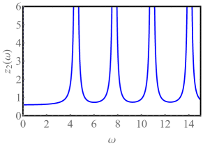
Figure 4: The function $z_{2}(\omega)$ vs. $\omega$ from (76). It has an infinite number of branches, but only the first branch corresponds to the optimal path. For this branch $z_{2}(\omega)$ diverges at $\omega=\omega^{*}=4.49341\dots$, which is the smallest positive root of the equation $\tan\omega=\omega$.

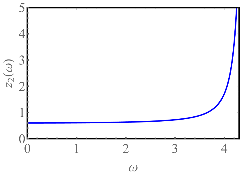
(a)

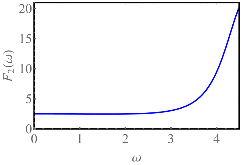
(b)

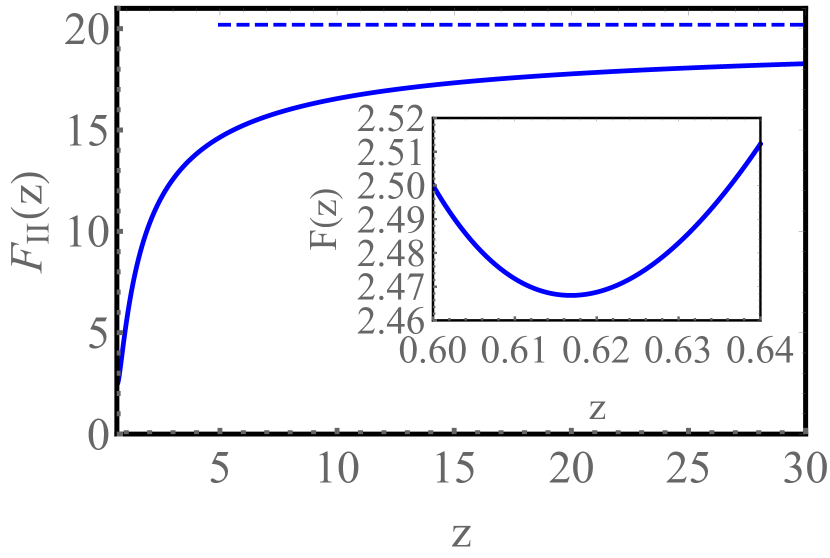
(c)

Figure 5: (a) The function $z_{2}(\omega)$ vs. $\omega$ from (76). It increases monotonically from $z_{2}(0)=3/5$ and diverges as $\omega$ approaches $\omega^{*}=4.49341$. (b) The function $F_{2}(\omega)$ vs. $\omega$, as defined by (77). It starts from $F_{2}(0)=5/2$, slightly decreases [see the inset in (c)], and then grows monotonically until $\omega=\omega^{*}=4.49341\dots$, reaching the value $F_{2}(\omega^{*})=(\omega^{*})^{2}=20.1907\dots$. (c) The function $F_{\rm II}(z)$ vs. $z$ , defined for $3/5\leq z<\infty$ and described in a parametric form by Eqs. (77) and (76). The horizontal dashed line is the large-$z$ asymptote $F_{\rm II}(z\to\infty)=(\omega^{*})^{2}=20.1907\dots$. The function $F_{\rm II}(z)$ reaches a minimum value $\pi^{2}/4$ at $z=\pi^{2}/16=0.61685\dots$, see the inset.

Note that the function $z_{2}(\omega)$ in (76) has multiple branches, see Fig. 4. As a result, for a fixed $z=z_{2}(\omega)$, there are multiple solutions for $\omega$. The function, associated with the first branch in Fig. 4, diverges at $\omega=\omega^{*}=4.49341\dots$, which is the smallest positive root of the equation $\tan\omega=\omega$, corresponding to a pole in Eq. (76). As one can show, the solutions, corresponding to the other branches, lead to larger values of the action $s=(1-X)F_{2}(\omega)$ for a fixed $X$, where $F_{2}(\omega)$ is given in (77). Hence, for the optimal (least action) path, we must select the first branch in Fig. 4, i.e. restrict ourselves to $0\leq\omega\leq\omega^{*}$. In this range of $\omega$ the function $z_{2}(\omega)$ is monotonically increasing, see Fig. 5(a), with the limiting behaviors

$$z_{2}(\omega)\simeq\begin{cases}&\frac{3}{5}+\frac{\omega^{2}}{175}+\ldots\,,\quad\quad\omega\to 0,\\ \\ &\frac{1}{4\,(\omega^{*}-\omega)^{2}}+\ldots\,,\quad\quad\omega\to\omega^{*}\,.\end{cases}$$ (78)

The function $F_{2}(\omega)$ vs. $\omega$ is plotted in Fig. 5(b). It starts from $F_{2}(0)=5/2$, first decreases with increasing $\omega$, reaches a minimum value $\pi^{2}/4$ at $\omega=\pi/2$ and then grows monotonically untill $\omega=\omega^{*}$. It has the limiting behaviors

$$F_{2}(\omega)\simeq\begin{cases}&\frac{5}{2}-\frac{\omega^{2}}{42}+\ldots\,,\quad\quad\omega\to 0,\\ \\ &(\omega^{*})^{2}-4\,\omega^{*}(\omega^{*}-\omega)+\ldots\,,\quad\quad\omega\to\omega^{*}\,.\end{cases}$$ (79)

The scaling function $F_{\rm II}(z)$ for $z\geq 3/5$, determined parametrically by Eqs. (77) and (76), is plotted in Fig. 5(c). As $z\to\infty$, $F_{\rm II}(z)$ approaches the constant $(\omega^{*})^{2}=20.1907\dots$. The limiting behaviors of $F_{\rm II}(z)$ are given by

$$F_{\rm II}(z)\simeq\begin{cases}&\frac{5}{2}-\frac{175}{42}\,(z-\frac{3}{5})+\ldots\,,\quad\quad z\to\frac{3}{5}\,,\\ \\ &(\omega^{*})^{2}-\frac{2\,\omega^{*}}{\sqrt{z}}+\ldots\,,\quad\quad z\to\infty\,.\end{cases}$$ (80)

We will refer to the solution for $z\geq 3/5$ as branch II. Here the optimal path $\phi(\tau)$ is monotonic on the time interval $\tau\in[0,1]$ for $0\leq\omega<\pi$, and non-monotonic for $\pi<\omega<\omega^{*}$.

IV.0.3 Summary

To summarize the results of this section, the joint probability $P(x,y,t)$ at short times, as predicted by the OFM at $1-X\ll 1$ and $|Y|\ll 1$, is given by Eq. (18) with the self-similar rate function

$$s(X,Y)=(1-X)\,F\left(\frac{1-X}{Y^{2}}\right)\,,$$ (81)

where

$$F(z)=\begin{cases}&\!\!\!F_{\rm I}(z),\;\frac{1}{2}\leq z\leq\frac{3}{5},\;\text{Eqs.~{}(\ref{zw_2.1}) and~{}(\ref{Fz_2.1})},\\ \\ &\!\!\!F_{\rm II}(z),\;z\geq\frac{3}{5},\;\text{Eqs.~{}(\ref{zw.1}) and~{}(\ref{Fz.1})}.\end{cases}$$ (82)

The branches I and II of the scaling function $F(z)$ join smoothly at $z=3/5$, where $F(z)=5/2$. The asymptotic behaviors of $F(z)$ are the following:

$$F(z)\simeq\begin{cases}&\frac{1}{8\,(z-1/2)}+\ldots,\quad\quad z\to 1/2,\\ \\ &(\omega^{*})^{2}-\frac{2\,\omega^{*}}{\sqrt{z}}\ldots\quad\quad z\to\infty.\end{cases}$$ (83)

where $\omega^{*}=4.49341\dots$ is the smallest positive root of the equation $\tan\omega=\omega$. Figure 6 shows a plot of $F(z)$ over the full range $z\geq 1/2$.

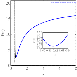
Figure 6: The scaling function $F(z)$ in the full range $z\geq 1/2$, obtained by combining $F(z)=F_{\rm I}(z)$ for $1/2\leq z\leq 3/5$ (branch I: the left one) and $F(z)=F_{\rm II}(z)$ for $z\geq 3/5$ (branch II: the right one). The horizontal dashed line is the large-$z$ asymptote $F(z\to\infty)=(\omega^{*})^{2}=20.1907\dots$. The vertical dashed line is the asymptote $z=1/2$. The two branches join smoothly at $z=3/5$, where $F(z)=5/2$. $F(z)$ reaches the minimum value $\pi^{2}/4$ at $z=\pi^{2}/16=0.61685\dots$, see the inset.

Figure 7: The isolines $s=0.1$, $0.2$, $1$ and $2$ of the rate function $s(X,Y)$ near $X=1$ and $Y=0$, as described by Eq. (81). The dotted line $|Y|=\sqrt{(5/3)(1-X)}$ is the boundary between the two branches I and II. The dashed line corresponds to the boundary of support of the distribution $|Y|=\sqrt{2(1-X)}$, which is the leading-order approximation, close to $X=1$ and $Y=0$, to the exact boundary of support $X^{2}+Y^{2}=1$. The rate function in the region $Y<0$ (not shown) is symmetric, with respect to $Y=0$, to the rate function in the region $Y>0$.

In its turn, Fig. 7 shows a contour plot of the rate function $s(X,Y)$, described by Eq. (75). There is a single point $(X=1,\,Y=0)$ where $s=0$. This point corresponds to the trivial (noiseless) optimal path $\phi(t)=0$. Then there are nested contours with increasing values of $s$ as one moves away from the point $(X=1,\,Y=0)$. The OFM solution exists only for $z>1/2$, that is for $Y^{2}<2(1-X)$. Using the asymptotics of $F(z)$ in the first line of (83), we see that, as $z\to 1/2$ from above, $s(X,Y)$ in Eq.(81) diverges:

$$s(X,Y)\simeq\frac{1-X}{8(z-1/2)}\,,\quad\text{where}\quad z=\frac{1-X}{Y^{2}}\,.$$ (84)

Consequently, the joint distribution $P(x,y,t)$ vanishes at $z=1/2$ extremely fast, via an essential singularity:

$$P(X,Y,t) \sim \exp\left[-\frac{16(1-X)}{Dt(z-1/2)}\right]\,.$$ (85)

Indeed, Fig. 7 shows a very steep growth of $s$ as we approach the limiting parabola $Y^{2}=2(1-X)$. For $z\leq 1/2$, that is at $Y^{2}>2(1-X)$, $P(x,y,t)$ is identically zero. All these features are in agreement with the exact analysis in the Introduction. In particular, close to $X=1$ and $Y=0$, the parabola $Y^{2}=2(1-X)$ is nothing but the leading-order approximation to the exact boundary of support of the joint distribution: the circle $X^{2}+Y^{2}=1$.

The self-similarity of the rate function (81) close to the zero-noise point is a natural consequence of an invariance property of the governing equations (29), (56) and (57) and the homogeneous boundary conditions (32). Under a stretching transformation $\phi\to c\,\phi$, where $c=\text{const}$, $s$ becomes $c^{2}s$, $1-X$ becomes $c^{2}(1-X)$, and $Y$ becomes $c\,Y$. As a result, both $s/(1-X)$ and $(1-X)/Y^{2}$ remain invariant, leading to the self-similar structure of $s(X,Y)$.

Overall, the applicability conditions of our asymptotic (18) and (81) of the joint distribution $P(x,y,t)$ are

$$Dv_{0}t^{2}\ll v_{0}t-x\ll v_{0}t\quad\text{and}\quad|y|\ll v_{0}t\,,$$ (86)

where the strong inequality $Dv_{0}t^{2}\ll v_{0}t-x$ guarantees that the action $S$ from Eq. (26) is much larger than unity. Equations (18) and (81) become asymptotically exact if we take the limits of $Dt\to 0$, $1-X\to 0$ and $Y\to 0$ while keeping the ratio $z=(1-X)/Y^{2}$ constant.

Finally, in Appendix A we show that the OFM prediction (18) and (81) for $P(x,y,t)$ in the vicinity of the point $(X=1,\,Y=0)$ perfectly agrees, at $Dv_{0}t^{2}\ll v_{0}t-x$ with the “near tail” of the expression for the joint distribution of typical fluctuations, derived by a different method in Ref. Basu2018 .

V Summary and discussion

Even a single active Brownian particle (ABP) on the plane exhibits unusual and non-intuitive properties. Here we studied the position statistics of the ABP at short times, when the initial conditions are still important, and the activity aspects are the most pronounced. We employed the optimal fluctuation method (OFM), which is well suited for studying large deviations of the position coordinates $x$ and $y$ of the ABP from their expected values. Besides the large deviation functions themselves, the OFM predicts important additional observable quantities: the optimal paths of the particle, conditioned on reaching specified values of the coordinates.

At all times, the joint distribution $P(x,y,t)$ has a compact support, the boundary of which is a uniformly expanding circle $x^{2}+y^{2}=v_{0}^{2}t^{2}$. The circumference of this circle includes the zero-noise point $(x=v_{0}t,\,y=0)$, where $P(x,y,t)$ has its maximum. The joint distribution vanishes in all other points of the circumference and outside of the circle.

Returning to short times: we showed that, close to the zero-noise point, the logarithm of $P(x,y,t)$ has an interesting self-similar structure, see Eqs. (18) and (81). This joint distribution matches smoothly with the tail of the joint distribution of typical fluctuations of $x$ and $y$, previously found by a different method in Ref. Basu2018 . Determining the complete joint statistics of $x$ and $y$ inside the expanding circle is left for a future work. Here we determined the complete marginal $x$- and $y$-distributions, see Secs. III.1 and III.2. One important feature of the marginals is that they vanish extremely fast, via essential singularities, at the edges of their support: at $x=-v_{0}t$ for the $x$-marginal, and at $y=\pm v_{0}t$ for the $y$-marginal. Since the corresponding $x$- and $y$- OFM actions diverge there, the essential singularities are not limited to short times and are expected to hold at all times. These large-deviation features are informative fingerprints of the short-time dynamics at long times, see also Ref. Basu2019 .

Appendix A Matching of the typical behavior of $P(x,y,t)$ with its large deviation form obtained via OFM

In Sec. IV we employed the OFM to evaluate, up to a pre-exponential factor, the joint distribution $P(x,y,t)$ at short times near $X=1$ and $Y=0$. The results are given by Eqs. (18) and (81), and they involve two branches of solution, I and II. Here we show that these results match perfectly with the left tail of the expression for $P(x,y,t)$, which describes typical fluctuations of $x$ and $y$ and was obtained, by a different method, in Ref. Basu2018 .

To see this, we consider Eq. (8) of Ref. Basu2018 , where the double Laplace transform of the joint distribution in the region of typical fluctuations was computed at short times near $x=v_{0}\,t$ and $y=0$. More precisely, it was shown in Ref. Basu2018 that for $Dt\ll 1$, and setting $x-v_{0}t\sim t^{2}$ and $y\sim t^{3/2}$, the joint distribution in this typical regime takes the scaling form as in (11). [which of course is compatible with the exact scaling behavior (20)]. The double Laplace transform of the scaling function ${\tilde{P}}(a_{1},a_{2})$ as computed explicitly using path integral method Basu2018

$$\int\int{\tilde{P}}(a_{1},a_{2})\,e^{-p_{1}a_{1}-p_{2}a_{2}}\,da_{1}\,da_{2}=\frac{\exp\left[p_{2}^{2}\,C(p_{1})\right]}{\sqrt{\cosh\sqrt{2p_{1}}}}\,,$$ (87)

where

$$C(p_{1})=\frac{1}{4\,p_{1}}\,\left(1-\frac{\tanh\sqrt{2p_{1}}}{\sqrt{2p_{1}}}\right)\,.$$ (88)

Inverting formally this Laplace transform, we get

$${\tilde{P}}(a_{1},a_{2})=\int\frac{dp_{1}}{2\pi i}\frac{e^{a_{1}p_{1}}}{\sqrt{\cosh\sqrt{2p_{1}}}}\int\frac{dp_{2}}{2\pi i}e^{p_{2}a_{2}+p_{2}^{2}\,C(p_{1})}\,,$$ (89)

where the integrals are over the Bromwich contours in the complex $p_{1}$ and the complex $p_{2}$ planes, respectively. The integration over $p_{2}$ can be performed exactly as it is just a Gaussian integral, leading to a single Laplace integral in the complex $p_{1}$ plane,

$${\tilde{P}}(a_{1},a_{2})=\int\frac{dp_{1}}{2\pi i}\frac{e^{a_{1}p_{1}-a_{2}^{2}/{4\,C(p_{1})}}}{\sqrt{4\,\pi\,C(p_{1})\,\cosh\sqrt{2p_{1}}}}\,,$$ (90)

where $C(p_{1})$ is given in (88). It is convenient to rewrite this integral in a more suggestive form

$${\tilde{P}}(a_{1},a_{2})=\int\frac{dp_{1}}{2\pi i}\frac{e^{-\frac{a_{1}}{2}\,\mathcal{F}(p_{1},z)}}{\sqrt{4\,\pi\,C(p_{1})\,\cosh\sqrt{2p_{1}}}}\,,$$ (91)

where we set

$$\mathcal{F}(p_{1},z)=\frac{1}{4\,z\,C(p_{1})}-2\,p_{1}\quad{\rm and}\quad z=\frac{a_{1}}{2\,a_{2}^{2}}\,.$$ (92)

So far Eqs. (91) and (92) are exact. It remains to perform the complex integral over $p_{1}$ in (91). The exact evaluation of this integral seems difficult. However, for large $a_{1}$ and $a_{2}$, with the ratio $z=a_{1}/(2\,a_{2}^{2})$ fixed, we can evaluate the integral by the saddle point method. The saddle point $p_{1}^{*}$ in the complex $p_{1}$ plane is obtained from the saddle-point equation

$$\frac{\partial\mathcal{F}(p_{1},z)}{\partial p_{1}}\Big{|}_{p_{1}=p_{1}^{*}}=0\,.$$ (93)

By analyzing (93), one can see that there is a saddle point for all $z\geq 1/2$. For $1/2\leq z\leq 3/5$, the saddle point occurs at a real positive $p_{1}$. Setting $p_{1}=w^{2}/2$, we find, after some algebra, that the saddle point equation (93) exactly coincides with (67) for the branch I of the OFM solution. The associated saddle point action $\mathcal{F}(w^{2}/2,z)$ yields the OFM function $F_{1}(w)$ for branch I in (68). Consequently, the tail of the joint distribution $P(x,y,t)$ of the typical fluctuations, for large $a_{1}$ and $a_{2}$ but with $z=a_{1}/(2\,a_{2}^{2})$ fixed, behaves (up to a pre-exponential factor) as

$$P(x,y,t)\sim\exp\left[-\frac{a_{1}}{2}\,\mathcal{F}\left(\frac{w^{2}}{2},z\right)\right]\,.$$ (94)

We recall that $a_{1}=(v_{0}\,t-x)/(v_{0}\,D\,t^{2})$ and $a_{2}=y/(v_{0}\,\sqrt{2\,D}\,t^{3/2})$. Therefore,

$$z=\frac{a_{1}}{2\,a_{2}^{2}}=\frac{v_{0}\,t\,(v_{0}\,t-x)}{y^{2}}\,.$$ (95)

In terms of the rescaled positions $X$ and $Y$ we obtain

$$z=\frac{1-X}{Y^{2}}\,,$$ (96)

which coincides with the scaling ratio, defined in (64). Similarly, the factor $a_{1}/2$ inside the exponent in (94) reads

$$\frac{a_{1}}{2}=\frac{1}{2Dt}\,(1-X)\,.$$ (97)

As a result, the tail of the joint distribution $P(x,y,t)$, describing the typical fluctuations, matches exactly with the OFM tail for $1/2\leq z\leq 3/5$.

Similarly, for $z\geq 3/5$, it turns out that the saddle point of (93) is on the negative side of the real $p_{1}$ axis. Setting $p_{1}=-\omega^{2}/2$, and carrying out exactly the same analysis as above, one can reconstruct the OFM solution for branch II, i.e., for $\lambda_{1}\geq 0$. Therefore, the matching between the asymptotics of the joint distributions $P(x,y,t)$ for the typical fluctuations and for the large deviations (the latter described by the OFM) occurs for all $z\geq 1/2$.

Appendix B Asymptotics of the marginal distributions from the joint distribution

Here we show how one can obtain the exponential asymptotic (41) of the near tail of $p_{x}(x,t)$, and the Gaussian asymptotic (52) of $p_{y}(y,t)$, from the OFM expressions (18) and (81) for the joint distribution $P(x,y,t)$ near the point $(x=v_{0}t,\,y=0)$.

The marginal distribution $p_{x}(x,t)$ is given by the integral of $P(x,y,t)$ over $y$. At short times this integral can be evaluated by the saddle-point method. Working with our OFM expressions, which were derived up to pre-exponential factors, we should ignore any such factors in the calculation. We obtain, therefore,

$$p_{x}(x,t)\sim\int\limits_{-\sqrt{2(1-X)}}^{\sqrt{2(1-X)}}dY\,\exp\left[-\frac{1-X}{2Dt}\,F\left(\frac{1-X}{Y^{2}}\right)\right].$$ (98)

A change of the integration variable from $Y$ to $z=(1-X)/Y^{2}$ brings us to

$$p_{x}(x,t)\sim\int_{0}^{\infty}dz\,\exp\left[-\frac{1-X}{2Dt}\,F(z)\right]\,$$ (99)

where we ignored all pre-exponential factors, both inside and outside the integrals. The saddle point is at $z=\pi^{2}/16$, where $F(z)=F_{\rm{II}}(z)$ has its minimum value $\pi^{2}/4$, and we obtain

$$p_{x}(x,t)\sim\exp\left[-\frac{\pi^{2}(1-X)}{8Dt})\right]\,.$$ (100)

Back to the variable $x$, this expression coincides with the near-tail asymptptic (41).

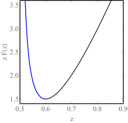
Figure 8: A plot of the function $zF(z)$, where $F(z)$ is defined in (82).

The marginal distribution $p_{y}(y,t)$ is given by the integral of $P(x,y,t)$ over $x$, and we obtain

$$p_{y}(y,t)\sim\int\limits_{-1}^{1-Y^{2}/2}dX\,\exp\left[-\frac{1-X}{2Dt}\,F\left(\frac{1-X}{Y^{2}}\right)\right].$$ (101)

The lower integration limit $-1$ is of course beyond the applicability domain of our $P(x,y,t)$, but this fact is inconsequential, because at short times the integral is dominated by a close vicinity of the upper integration limit. Going over from $X$ to $z$, we obtain

$$p_{y}(y,t)\sim\int_{1/2}^{\infty}dz\,\exp\left[-\frac{Y^{2}}{2Dt}zF(z)\right]\,.$$ (102)

Now the saddle point is the minimum point of the function $zF(z)$. A plot of the function $zF(z)$ vs. $z$ is shown in Fig. 8. The minimum value $3/2$ is achieved at $z=3/5$, that is at the matching point of the two branches $F_{\rm{I}}(z)$ and $F_{\rm{II}}(z)$. As a result,

$$p_{y}(y,t)\sim\exp\left(-\frac{3Y^{2}}{4Dt}\right).$$ (103)

This Gaussian can be properly normalized, leading to Eq. (52).

References

- (1) P. Romanczuk, M. Bär, W. Ebeling, B. Lindner, and L. Schimansky-Geier, Eur. Phys. J. Special Topics 202, 1 (2012).
- (2) M. C. Marchetti, J. F. Joanny, S. Ramaswamy, T. B. Liverpool, J. Prost, M. Rao, and R. Aditi Simha, Rev. Mod. Phys. 85, 1143 (2013).
- (3) C. Bechinger, R. Di Leonardo, H. Löwen, C. Reichhardt, G. Volpe, and G. Volpe, Rev. Mod. Phys. 88, 045006 (2016).
- (4) É. Fodor, and M. C. Marchetti, Physica A 504, 106 (2018).
- (5) A. P. Solon, M. E. Cates, and J. Tailleur, Eur. Phys. J. Special Topics 224, 1231 (2015).
- (6) R. Grossmann, F. Peruani, and M. Bär, Eur. Phys. J. Special Topics 224, 1377 (2015).
- (7) P. Pietzonka, K. Kleinbeck, and U. Seifert, New J. Phys. 18, 052001 (2016).
- (8) C. Kurzthaler, C. Devailly, J. Arlt, T. Franosch, W. C. K. Poon, V. A. Martinez, and A. T. Brown, Phys. Rev. Lett. 121, 078001 (2018).
- (9) U. Basu, S. N. Majumdar, A. Rosso, and G. Schehr, Phys. Rev. E 98, 062121 (2018).
- (10) T. GrandPre, and D. T. Limmer, Phys. Rev. E 98, 060601(R) (2018).
- (11) U. Basu, S. N. Majumdar, A. Rosso, and G. Schehr, Phys. Rev. E 100, 062116 (2019).
- (12) A. Shee, A. Dhar, and D. Chaudhuri, preprint arXiv: 2002.01815
- (13) D. Mumford, Elastica and Computer Vision, in Algebraic Geometry and its Applications, edited by C. L. Bajaj (Springer, New York, 1994).
- (14) A. Grosberg and H. Frisch, J. Phys. A: Math. Gen. 36, 8955 (2003).
- (15) B. Meerson, J. Stat. Mech. 013210 (2019).
- (16) N. R. Smith and B. Meerson, J. Stat. Mech. 023205 (2019).
- (17) B. Meerson and N. R. Smith, J. Phys. A: Math. Theor. 52, 415001 (2019).
- (18) T. Agranov, P. Zilber, N. R. Smith, T. Admon, Y. Roichman and B. Meerson, Phys. Rev. Res. 2, 013174 (2020).
- (19) S. N. Majumdar and B. Meerson, J. Stat. Mech. 023202 (2020).
- (20) L. Elsgolts, Differential Equations and the Calculus of Variations (Mir, Moscow, 1977).
- (21) There is also a monotone-decreasing solution, symmetric to this one with respect to the -axis. It has exactly the same action.