Towards a self-consistent Boltzmann’s kinetic model of fluid turbulence

Abstract

A closure for the effective relaxation time of the Boltzmann-BGK kinetic equation for fluid turbulence is presented, based on a double-averaging procedure over both kinetic and turbulent fluctuations. The resulting effective relaxation time appears to agree with values obtained via a renormalization group treatment of the Navier-Stokes equation only at low values of $k/T$, the ratio of turbulent kinetic energy to fluid temperature. For $k/T>0.1$ the kinetic treatment delivers a significantly longer effective relaxation time.

1 Introduction

The basic equations of fluid mechanics are known for two centuries, and yet, fluid turbulence keeps standing as one of the most challenging and compelling problems in modern science, holding back progress across many fluid-related disciplines and application in science and engineering [1].

Computer simulations have moved great lengths in the direction of unraveling the complexity of fluid flows, and yet, even most powerful foreseeable (non-quantum) computers fall short of providing access to the direct simulation of most flows of practical interest, such as a full car or airplane, not to mention geophysics, astrophysics and cosmology.

Hence, major efforts are devoted to the task of devising the effects of the small unresolved scales on the large and resolved ones, an art known as turbulence modeling (TM) [2].

A central idea of TM is the notion of eddy viscosity, whereby the collective degrees of freedom of turbulence ("eddies") are treated in full analogy with molecules in kinetic theory [3]. This means that the large eddies experience a sort of Brownian motion due to the erratic collisions with small eddies, leading to the notion of "eddy viscosity". This concept has proved extremely valuable but suffers of a basic flaw, namely the assumption of scale separation between short and large eddies. While suitable for molecules, such scale-separation fails for fluid turbulence, owing to the continuum spectrum of turbulent eddies.

Thus, what one needs is a theoretical and computational framework capable of dealing with the non-perturbative aspects of eddy interactions across scales of motion, and most notably with the interactions between eddies of nearby size.

Kinetic theory is ideally positioned to offer such a framework, since the Boltzmann equation requires no separation between micro and macroscopic scales. In more technical terms, it applies at any value of the Knudsen number, leading to hydrodynamics in the limit of zero Knudsen numbers.

However, the Boltzmann equation has been traditionally disregarded by the turbulence community mainly account of its computational complexity: why solving a $(6+1)$-dimensional equation to attack a problem which lives in $(3+1)-d$ only?

Over the last decade, this position has been revisited thanks to the vigorous development of the lattice Boltzmann (LB) method, which is based on a minimal Boltzmann equation, living in a discrete and uniform lattice [4].

More precisely, turbulence models based on suitable extensions of the LB have been developed and applied to a variety of ideal and real-life turbulent flows [5, 6, 7].

Notwithstanding their practical success, such an approach has been criticised on account of lack of self-consistency, namely the fact of coupling the LB to a macroscopic equations for the fluctuating kinetic energy, which is derived from coarse-graining of the macroscopic fluid equations.

In this paper we (partially) mend this weakness by showing that a very simple kinetic closure leads to a formulation very similar to the one obtained in the macroscopic approach.

2 Kinetic equation for turbulent eddies

The main idea of the kinetic approach to fluid turbulence is to coarse-grain the Boltzmann kinetic equation before taking the Chapman-Enskog limit from the kinetic to the hydrodynamic level [8, 5, 6]. This contrasts with the standard hydrodynamic approach , which consists in coarse-graining the Navier-Stokes equations.

Symbolically:

$$U_{h}(x;t)={\mathcal{P}}_{x}\cdot{\mathcal{P}}_{v}\cdot f(x,v;t)$$ (1)

for the hydrodynamic approach, versus the kinetic one:

$$U_{k}(x;t)={\mathcal{P}}_{v}\cdot{\mathcal{P}}_{x}\cdot f(x,v;t).$$ (2)

In the above, ${\mathcal{P}}_{x}$ denotes a space-filtering projection operator, while ${\mathcal{P}}_{v}$ denotes the velocity projector associated with Chapman-Enskog asymptotics. In full generality, we expect the two projectors to commute only whenever the coarse-grained mean-free path $\Lambda_{m}$ remains sufficiently smaller than the lattice spacing $\Delta$, i.e.

$$Kn_{\Delta}=\Delta/\Lambda_{m}\ll 1$$

This condition is tantamount to assuming a scale-separation between the resolved and unresolved eddies, an assumption that, while inevitable in the hydrodynamic picture, is guaranteed to fail for eddies in the vicinity of the lattice cutoff $\Delta$. This very plain observation highlights the potential of the kinetic approach to deliver a genuine new class of turbulence models, free of scale-separation assumptions, hence more suitable to handle strong non-equilibrium turbulence, as it typically occurs in the vicinity of solid boundaries.

To implement the above program, we start from the Boltzmann equation in single-time relaxation form (BGK) [9]:

$$\partial f=\frac{1}{\tau_{0}}(f^{eq}-f)$$

where $\partial\equiv\partial_{t}+v\partial_{x}$ is the Lagrangian derivative along the molecular velocity (streaming operator) and $\tau_{0}$ is the molecular relaxation time .

In the above $f(x,v;t)$ is the probability of finding a molecule at position $x$ with velocity $v$ at time $t$ and $f^{eq}$ is a local Maxwellian at temperature $T$ and average fluid velocity $u(x,t)$. Vector indices are relaxed for simplicity.

The basic coarse-grained kinetic quantities are defined as follows:

$$F\equiv<f>,$$ (3)

$$F^{eq}\equiv f^{eq}(<f>),$$ (4)

$$\delta F^{eq}\equiv<f^{eq}(f)>-f^{eq}(<f>)$$ (5)

the latter being the contribution of the nonlinear turbulent fluctuations $u^{\prime}=u-U$, $U=<u>$, $<u^{\prime}>=0$, to the coarse-grained equilibrium, brackets denoting ensemble averaging over turbulent fluctuations.

In the renormalization group language, one would like to understand how the Boltzmann-BGK equation transforms under the following rescaling:

$$x\to bx,\;t\to bt,\;u\to u,\;v\to v,\;\tau\to b^{\alpha}\tau$$ (6)

where $\tau_{R}\equiv b^{\alpha}\tau$ is the renormalised relaxation time, accounting for coarse-grained nonlinear contributions. In particular, if $\alpha>1$, the lattice Knudsen number increases in the large-scale limit, so that space filtering and the Chapman-Enskog expansion do not necessarily commute, thus leading to a potentially new class of kinetic turbomodels with no hydrodynamic counterpart [8, 10].

Formal coarse graining (filtering) of the kinetic equation delivers:

$$\partial F=-\frac{1}{\tau_{0}}(\delta F^{neq}+\delta F^{eq})$$ (7)

where we $\delta F^{neq}\equiv F-F^{eq}$ is the coarse-grained non-equilibrium and $\delta F^{eq}$ is the contribution from the nonlinear fluctuations of the fine-grained local equilibrium $f^{eq}$.

From the above, we formally derive the following "renormalised" relaxation time (RRT):

$$\frac{\tau_{R}}{\tau_{0}}=\frac{1}{1-R}$$ (8)

where we have set

$$R=\delta F^{eq}/\delta F^{neq}$$ (9)

In other words, the RRT depends only on the ratio between the turbulent and kinetic fluctuations. Note that in the absence of coarse-graining, $\delta F^{eq}=0$, and $\tau_{R}\to\tau_{0}$, as it should be by mere consistency.

Three distinguished regimes are apparent.

1) Contraction regime ($R<0$): the turbulent fluctuations carry an opposite sign as compared to the kinetic ones, so that the renormalized relaxation time is shorter than the bare one (contraction). This is an unlikely situation, which may eventually occur for supersmooth regimes, in which the velocity fluctuations scale superlinearly with the size of the eddies, $\delta u(l)\propto l^{1+\alpha}$, $\alpha>0$, so that $\tau(l)=l/\delta u(l)\sim l^{-\alpha}$.

2) Dilatation regime ($0<R<1$): the turbulent fluctuations carry the same sign as the non-equilibrium ones, but they are smaller in amplitude. Consequently, the RRT exceeds the bare relaxation time and diverges in the limit $R\to 1$.

The relation (8) shows that largest RRT’s arise in connection to turbulent fluctuations getting close to the kinetic ones, yet smaller. The physical interpretation is that in the range $0<R<1$, the renormalised equilibrium $<f^{eq}>$ gets closer to the actual coarse-grained distribution $<f>$ than the bare coarse-grained equilibrium $f^{eq}(<f>)$, which is tantamount to a dilatation of the renormalised relaxation time (RRT). In this regime scale separation breaks-down and the kinetic approach is expected to deliver genuinely new results.

Unstable regime ($R>1$): the turbulent fluctuations still carry the same sign as kinetic ones, but now they are larger in amplitude. As a result, $\tau_{R}$ becomes formally negative, which hints at an instability, since it is as if in order to attain the equilibrium, the system should go back in time, which manifestly it cannot do. While we are in no position to assess the realizability of such regime, we simply observe that occasional instabilities are definitely part of the picture in the case of non-equilibrium turbulence (gusts of intermittency).

Leaving a more detailed inspection of these three regimes to a future publication, we next proceed to a quantitative assessment of both turbulent and kinetic fluctuations.

3 Turbulent fluctuations: coarse-grained equilibria

Under the assumption of ergodicity, coarse-graining can be formulated as a space-time filter of the form:

$$F(x,v,t)\equiv<f>=\int K(x-x^{\prime},t-t^{\prime})f^{eq}(x^{\prime},v,t^{\prime})dx^{\prime}dt^{\prime}$$

In practice, this all but a convenient procedure, for it requires homogeneous directions to average upon, which are hardly available in real-life geometries [11].

Hence, we take a different route, first developed by Yakhot [12, 13], which replaces spacetime averaging with ensemble averaging in kinetic space. More precisely, one decomposes the molecular velocity as follows:

$$v=U+u^{\prime}+v^{\prime}\equiv V+u^{\prime}$$

where $u^{\prime}$ are the turbulent fluctuations, $v^{\prime}$ are the kinetic ones and we have set $V=U+v^{\prime}$.

By ergodicity, we assume that the filtering in space can be replaced by a (functional) average over the turbulent fluctuations, namely:

$$F(U+v^{\prime})=\int f(U+v^{\prime}+u^{\prime})P(u^{\prime}|U)du^{\prime}$$

Next we make the plausible assumption that the one-point velocity fluctuations are gaussian distributed with variance $k=<u^{\prime 2}>/2$, the "turbulent temperature", i.e., in $d$ spatial dimensions:

$$P(u^{\prime}|U)=(2\pi k)^{-d/2}e^{-u^{\prime 2}/2k}$$ (10)

Note that for one-point fluctuations in homogenous turbulence, this assumption is a pretty safe one.

Since the local equilibrium is gaussian, and so is the one-point distribution, the above integral can be performed analytically, to deliver a "Doppler" shifted gaussian with temperature $T\to T+k$, where $k=<u^{\prime 2}>/2$ is the turbulent kinetic energy (we have set $k_{B}=1$ and unit density since we deal with incompressible flows).

Thus, the coarse-grained BGK equation reads as follows:

$$\partial F=\frac{1}{\tau_{0}}(F^{eq}_{k+T}-F)$$ (11)

which looks exactly the same as the original one, only with a Doppler shifted equilibrium.

The equation is not closed, though, as it requires the dynamics of the turbulent kinetic energy $k$.

This can be derived by multiplying the BGK equation by $u^{\prime 2}/2$ and performing the double integration upon $v^{\prime}$ and $u^{\prime}$, namely

$$k(x,t)=<<u^{\prime 2}>>=\int F(U+u^{\prime}+v^{\prime};x,t)P(u^{\prime}|U)u^{\prime 2}du^{\prime}dv^{\prime}.$$ (12)

The resulting equation is [13]:

$$\partial_{t}k+U\partial_{x}k+\partial_{x}<u^{\prime 3}>=-\frac{1}{\tau_{0}}(k-k_{eq})$$ (13)

Performing the algebra and setting cross-correlation terms $<u^{\prime}u^{\prime}v^{\prime}>$ to zero (true only at equilibrium) we obtain $k_{eq}\sim kT/(k+T)=k/(1+k/T)$. This interpolates between $k$ in the limit $k/T<<1$ and $T$ in the opposite limit $k/T>>1$, the former being usually the relevant case for fluid turbulence.

The skewness term $<u^{\prime 3}>$, requires a non-equilibrium closure, examples of which can be found in [12].

Here, however, we wish to pursue a different goal, namely, in line with RG ideas, leave the coarse-grained equilibria invariant and formulate a kinetic closure for the the renormalized relation time $\tau_{R}$.

Based on the above, by definition:

$$\phi(c,\kappa)\equiv\frac{\delta F^{eq}}{F^{eq}}=\frac{(T+k)^{-3/2}e^{-w^{2}/2(T+k)}}{T^{-3/2}e^{-w^{2}/2T}}-1$$ (14)

where $w=v-U$ is the coarse-grained peculiar speed.

A simple rearrangement yields:

$$\phi(c,\kappa)=\frac{e^{\frac{c^{2}}{2}\frac{\kappa}{1+\kappa}}}{(1+\kappa)^{3/2}}-1$$ (15)

where we have defined $\kappa\equiv k/T$ and $c\equiv w/T^{1/2}$.

It can be readily checked that such quantity hardly exceeds $1$, other than for superthermal excitations with $c\gg 1$. Since such superthermal excitations are exponentially suppressed in the molecular fluid, we conclude that $\delta F^{eq}/F^{eq}$ is generally well below $1$ (see Figure 1).

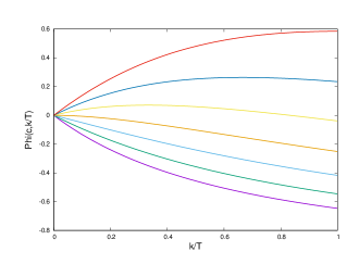
Figure 1: The ratio of turbulent fluctuations to the bare coarse-grained equilibrium as a function of the parameter $k/T$ for different values of the peculiar speed $c^{2}=0,1,2,3,4,5,6$, top to bottom.

For instance, to order $\kappa^{2}$, we obtain:

$$<\delta F^{eq}/F^{eq}>=(1-(3/2)\kappa+(9/4)\kappa^{2})(1+\frac{<c^{2}>}{2}\frac{\kappa}{1+\kappa}+\frac{<c^{4}>}{8}\frac{\kappa^{2}}{(1+\kappa)^{2}})+O(\kappa^{4})$$

where brackets denote integration upon the peculiar velocity. By recalling that in $d=3$, $<c^{2}>=3$, and $<c^{4}>=9$, we obtain:

$$<\delta F^{eq}/F^{eq}>=-\frac{3}{4}\kappa^{2}+O(\kappa^{3})$$ (16)

Since $\kappa\sim 0.1$, this is of the order of $0.01$, thus showing that the scale-separation breaking regime $R\to 1$ is attained through nonequilibrium heterogeneity effects sligthly below such value.

A crucial caveat must be pointed out: the relation $<c^{2}>=3$ and $<c^{4}>=9$ only hold at equilibrium, which means that performing the average with the actual distribution delivers a linear contribution $(<c^{2}>-3)\kappa/2$. The ratio of non-equilibrium to equilibrium distribution scales like the Knudsen number, $Kn\equiv\tau_{R}\partial\sim\tau_{R}/\tau_{tur}$, where $\tau_{tur}$ is a typical turbulent time scale to be discussed in the next section.

In view of such observation, we finally write

$$\Phi\equiv<\delta F^{eq}/F^{eq}>=C_{1}\kappa-\frac{3}{4}\kappa^{2}+O(\kappa^{3})$$ (17)

where $C_{1}\sim Kn$. Hence, the linear contribution in $k/T$ is a genuine non-equilibrium effect.

4 Coarse-grained non-equilibrium

The denominator of eq (8), can be computed by solving the coarse-grained BGK equation in the form $(1+\tau_{R}\partial)F=F^{eq}$. This delivers:

$$\delta F^{neq}=-\{\frac{rz}{1+rz}\}F^{eq}$$ (18)

where we have defined $r=\tau_{R}/\tau_{0}$ and $z\equiv\tau_{0}\partial$ (the Knudsen operator).

Inserting (18) in (8), we obtain a self-consistent operator equation for the renormalized relaxation time $\tau_{R}$.

This is a fully non-local operator equation, since $z$ involves the streaming operator $\partial$, but we shall treat it as an ordinary number by invoking the correspondence rule $\partial=1/\tau_{tur}$, subscript "tur" standing for "turbulent".

By letting $\theta\equiv\tau_{tur}/\tau_{0}$, the relation (18) simplifies to

$$r-1=-(1+\theta)\frac{\phi}{1+\phi}$$ (19)

where we remind that $\phi\equiv\delta F^{eq}/F^{eq}$. Integration upon the peculiar velocity provides

$$r-1=-(1+\theta)\frac{\Phi}{1+\Phi}$$ (20)

where $\Phi=<\phi>$ and we have made the assumption $\phi\ll 1$.

The next task then is to pin down a concrete expression for the unknown timescale $\tau_{tur}$.

A natural correspondence rule is as follows:

$$\frac{1}{\tau_{tur}}={(\frac{1}{\tau_{l}^{2}}+\frac{1}{\tau_{s}^{2}})}^{1/2}$$ (21)

where $\tau_{l}=k/\epsilon$ is the local timescale of homogeneous turbulence and $\tau_{s}=1/S$ is the inhomogeneity scale, $S=\partial_{r}u$ being the shear rate. The ratio of the two, often denoted as strain parameter, $\eta=kS/\epsilon$ is a measure of non-equilibrium between eddies of different size, $\eta=0$ denoting the equilibrium case (no strain).

The above correspondence rule is tantamount to postulating that the time derivative in the streaming operator contributes a term $1/\tau_{l}$, where $\tau_{l}$ is a typical time scale of homogeneous turbulence, namely $\tau_{l}\sim k/\dot{k}$.

Likewise, it appears plausible to assume that the spatial derivative $v\partial_{x}$ contributes a term of order $1/\tau_{s}=S$ where $S\sim\partial_{x}U$ is the large-scale shear. The square is for the sake of positivity, but any higher even power would do.

Putting together the expressions (17) and (20), we we arrive at the following expression (in the limit $k/T\ll 1$):

$$\frac{\tau_{R}}{\tau_{0}}-1=\frac{C_{1}\kappa+C_{2}\kappa^{2}}{1+C_{1}\kappa+C_{2}\kappa^{2}}\;[1+\frac{\tau_{l}/\tau_{0}}{(1+\frac{\tau_{l}^{2}}{\tau_{s}^{2}})^{1/2}}]$$ (22)

where $C_{1}\sim Kn$ and $C_{2}\sim 3/4$.

Noting that the coefficient $C_{1}$ is proportional to the Knudsen number, hence depends on $\tau_{R}$ itself, we rearrange the above expression in the following form:

$$\frac{\tau_{R}}{\tau_{0}}-1=\frac{K_{1}\kappa+K_{2}\kappa^{2}}{1+K_{3}\kappa+O(\kappa^{2})}\;\frac{\tau_{l}/\tau_{0}}{(1+\frac{\tau_{l}^{2}}{\tau_{s}^{2}})^{1/2}}$$ (23)

where $K_{1}=\tau_{0}/\tau_{tur}$, $K_{2}=3/4$, $K_{3}=1+\tau_{0}/\tau_{tur}$ and we have made the the assumption $\tau_{0}/\tau_{tur}\ll 1$.

This is the main result of this paper, in that it provides a kinetic closure for the RRT‘in terms of the ratio $k/T$ and the turbulent timescale $\tau_{tur}$.

5 Comparison with Yakhot-Orszag renormalization group treatment

The above treatment suggest a general expression for the RRT, namely

$$r-1=\Psi^{eq}(k/T)\;\Psi^{neq}(\frac{\tau_{l}}{\tau_{0}},\frac{\tau_{s}}{\tau_{0}})$$ (24)

where $\Psi^{eq}$ and $\Psi^{neq}$ encode the effects of turbulent and kinetic fluctuations, respectively.

It is now instructive to inspect whether the corresponding expressions derived from a RG treatment of the Navier stokes equations i) fit in the above expressions, and if so, ii) whether the "universal" functions $\Psi^{eq}$ and $\Psi^{neq}$ are the same.

The Yakhot-Orszag expression of the renormalized relaxation time derived from a RG treatment of the Navier-Stokes equations, reads as follows [14]:

$$r_{YO}-1=C_{YO}\frac{k}{T}\frac{\tau_{l}/\tau_{0}}{\sqrt{1+\eta^{2}}}$$ (25)

where we have set $\eta=\tau_{s}/\tau_{l}=kS/\epsilon$, and the numerical constant is $C_{YO}\sim 0.08$.

Under the assumption $\tau_{tur}/\tau_{0}\gg 1$, the non-equilibrium component of the YO expression is exactly the same as the kinetic one, equation (21).

As to the equilibrium component, from (25) one reads off:

$$\delta F^{eq}/F^{eq}=\frac{C_{YO}k/T}{1-C_{YO}k/T}$$

In Fig 2 we compare the YO expression above with both kinetic expressions (22) (with $C_{1}=C_{YO}=0.08$) and (23) for two different values of $\theta\equiv\tau_{tur}/\tau_{0}=10,100$.

The figure shows that while all kinetic expressions provide a satisfactory agreement with the YO formulation for $k/T$ below about $0.1$, above such value the kinetic formulations predict a significantly larger relaxation time.

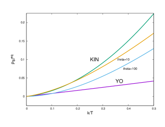
Figure 2: The equilibrium contribution to the renormalized relaxation rate: Yakhot-Orszag (YO), present derivation (KIN), namely expression 22 and 23 with $\theta=10,100$

.

6 Conclusion

We have derived an ab-initio kinetic expression for the renormalized relaxation rate as a function of the dimensionless ratios $k/T$ (turbulent Mach number) and turbulent time scales $\tau_{l}$ and $1/S$.

The kinetic expression shows strong similarity with the Yakhot-Orsag expression, with a much larger quadratic term in the parameter $k/T$. In the range $k/T<0.1$, the numerical values are comparable, but for larger values the kinetic relaxation time significantly exceeds the YO value. It would be interesting to explore the effect of the new expression (23) in hydrokinetic simulations of turbulent flows.

7 Acknowledgments

The author owes a huge debt of knowledge to Hudong Chen, Viktor Yakhot and to the late SA Orszag, a wonderful master and a much missed friend.

This paper was prepared on the occasion of the Simons Symposium "Universality: Turbulence across vast scales". The author is grateful to the Simons Foundation for financial support and great hospitality and to David Spergel and Phil Mocz for very stimulating discussions.

This research has also received funding from the European Research Council, under the European Union’s Horizon 2020 Framework Programme (No. FP/2014- 2020)/ERC Grant Agreement No. 739964 (COPMAT).

References

- [1] U. Frisch, Turbulence, Cambridge U.P., 1995
- [2] P.R. Spalart, Int. J. of Heat and Fluid Flow, 21(3),252 (2000)
- [3] J. Boussinesq, C. R. Acad. Sci. Paris, 71 389-93, (1870)
- [4] R. Benzi, S. Succi, M. Vergassola, Phys. Rep., 1992
- [5] H Chen, S Orszag, I Staroselsky and S Succi, J. Fluid Mech. 519 301, (2004)
- [6] H Chen, S Orszag and I Staroselsky, J. Fluid Mech. 658 294, (2010)
- [7] H Chen, S Kandasamy, S Orszag, R Shock, S Succi and V Yakhot, Science 301 633, (2003)
- [8] H Chen, S Succi and S Orszag, Phys. Rev. E Rap. Comm. 59 R2527, (1999)
- [9] PL Bhatnagar, E Gross and M Krook, Phys. Rev. 94 511, (1954)
- [10] S. Ansumali, I. Karlin, S. Succi, Physica A: Statistical Mechanics and its Applications, 338 (3-4), 379-394, (2001)
- [11] J. Larsson and Q. Wang, Phil. Trans. Roy. Soc. A 372: 20130329. http://dx.doi.org/10.1098/rsta.2013.0329, (2014).
- [12] V. Yakhot, S. Orszag, Turbulence models generators, arXiv.org > nlin > arXiv:0706.4451, (2007)
- [13] H. Chen, I. Staroselsky, V. Yakhot, Phys. Scr. T155, 014040 (2013)
- [14] V. Yakhot, S. Orszag, J. Sci. Comp. 1 (1), 3-51, (1986)