Higgs time crystal in a high-$T_{c}$ superconductor

Abstract

We propose to induce a time crystalline state in a high-$T_{c}$ superconductor, by optically driving a sum resonance of the Higgs mode and a Josephson plasma mode. The generic cubic process that couples these fundamental excitations converts driving of the sum resonance into simultaneous resonant driving of both modes, resulting in an incommensurate subharmonic motion. We use a numerical implementation of a semi-classical driven-dissipative lattice gauge theory on a three-dimensional layered lattice, which models the geometry of cuprate superconductors, to demonstrate the robustness of this motion against thermal fluctuations. We demonstrate this light-induced time crystalline phase for mono- and bilayer systems and show that this order can be detected for pulsed driving under realistic technological conditions.

I Introduction

Optical driving of solids constitutes a new method of designing many-body states. Striking examples of this approach include light-induced superconductivity [1, 2, 3] as well as optical control of charge density wave phases [4]. For these states, the carefully tuned light field either renormalises the phase boundary of the equilibrium phase, as is the case for light-induced superconductivity, or renormalises a near-by metastable state into a stable state of the driven system, as is the case for light-controlled charge density waves.

These observations are part of a larger effort to determine the steady states of periodically driven many-body systems. In a parallel development in cold atom systems, serving as well-defined many-body toy models, the generic regimes that were proposed, see Refs. [5, 6], firstly include renormalised equilibrium states, for which the above mentioned states are examples. Secondly, regimes beyond the equilibrium states emerge, in particular genuine non-equilibrium orders, which have no equilibrium counterpart, and only exist in the driven state. A striking example of a non-equilibrium order is time crystals [7, 8, 9, 10, 11, 12, 13], reported in systems such as ion traps or nitrogen-vacancy centers [14, 15]. Thirdly, for strong driving, chaotic states emerge. These different regimes are achieved for different driving amplitudes and driving frequencies, which constitutes the dynamical phase diagram of the system.

In this paper, we propose to create a light-induced time crystalline state in a high-$T_{c}$ superconductor. This advances light control of superconductors towards genuine non-equilibrium orders, and furthers time crystals in the solid state domain [16]. We characterise the observed non-equilibrium state as a time crystal based on the following criteria [12]: (i) A time crystal spontaneously breaks time-translation symmetry, that is, it exhibits a subharmonic response to the drive. (ii) The subharmonic response is robust against perturbations which respect the time-translation symmetry of the Hamiltonian. (iii) The subharmonic response emerges in a many-body system with a large number of locally coupled degrees of freedom, and it persists for an infinite time.

We call the novel dynamical phase a Higgs time crystal because we induce it via optical driving of a sum resonance of the Higgs mode and a Josephson plasma mode. The Higgs mode and the Josephson plasma mode correspond to the two fundamental collective excitations of a system with broken $U(1)$ symmetry and with an underlying approximate particle-hole symmetry. The Higgs mode is an amplitude oscillation of the order parameter, as depicted in Fig. 1(a) for the $|\psi|^{4}$ theory used in the following. The Higgs mode is a gapped excitation due to the increase of the potential energy in the radial direction. The Josephson plasma mode is a phase oscillation, as indicated. This mode also has a gapped excitation spectrum owing to the electromagnetic interaction of the system. Because of the approximate particle-hole symmetry, these two oscillations are orthogonal to each other [17, 18].

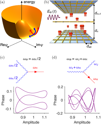
Figure 1: Exciting the Higgs and plasma modes. (a) Illustration of the free energy of a state with broken $U(1)$ symmetry. (b) Illustration of a driven cuprate superconductor modelled as a $U(1)$ gauge theory on an anisotropic lattice. In-plane dynamics is captured by discretising the condensate field in the $ab$-plane. (c) The Higgs mode can be excited resonantly with a driving frequency of $\omega_{\mathrm{dr}}\lesssim\omega_{\mathrm{H}}/2$, by utilising the non-linear coupling between the electromagnetic field and the Higgs field. Upper panel: Diagrammatic representation of the non-linear process. Lower panel: Exemplary dynamical portrait of the phase difference between the superconducting layers and the condensate amplitude in the steady state for 10 driving cycles at zero temperature. (d) We propose to utilise the same non-linear coupling to induce a time-crystalline state by driving the sum resonance of the system at $\omega_{\mathrm{dr}}=\omega_{\mathrm{H}}+\omega_{\mathrm{J}}$. The phase-space trajectories shown in the lower panels of (c) and (d) are obtained using a Josephson junction model for a monolayer cuprate with Higgs frequency $\omega_{\mathrm{H}}/2\pi\approx 6.3$ THz and plasma frequency $\omega_{\mathrm{J}}/2\pi\approx 16.0$ THz, see Table 1 for full parameter set.

To identify the Higgs time crystalline phase, we map out the dynamical phase diagram of optically driven high-$T_{c}$ superconductors as a function of the driving frequency $\omega_{\mathrm{dr}}$ and the driving amplitude $E_{0}$, which is shown in Fig. 2(a), for instance. The time crystalline state is induced by driving the superconductor via the non-linear coupling $\sim a^{2}h$ of the electromagnetic field $a$ and the Higgs field $h$. We demonstrate that driving at the frequency $\omega_{\mathrm{dr}}=\omega_{\mathrm{H}}+\omega_{\mathrm{J}}$ induces a time crystalline phase, where $\omega_{\mathrm{H}}$ is the Higgs frequency and $\omega_{\mathrm{J}}$ is the plasma frequency, as depicted in Fig. 1(d). We note that this non-linear coupling has been confirmed in conventional superconductors [19, 20, 21, 22], while a direct probe of the Higgs field is challenging due to its scalar nature. Further studies on the Higgs mode in high-$T_{c}$ cuprates and organic superconductors are reported in Refs. [23, 24, 25, 26, 27, 28, 29]. Persistent multi-frequency dynamics of the superconducting order parameter has been investigated in Ref. [30].

To describe the dynamics of optically driven superconductors, we develop a lattice gauge simulation that describes the motion of the order parameter of the superconducting state $\psi(\mathbf{r},t)$ and the electromagnetic field $\mathbf{A}(\mathbf{r},t)$. We first utilise our method to show how to induce the time crystalline state, and to determine its regime in the dynamical phase diagram. Furthermore, we demonstrate the robustness of the time crystalline phase against thermal fluctuations, and show that it can be realised and identified under pulsed operation.

II Three-dimensional lattice gauge model

We represent the layered structure of high-$T_{c}$ superconductors via the lattice geometry illustrated in Fig. 1(b). We note that this geometry of CuO₂ layers perpendicular to the $c$-axis has motivated a low-energy description of stacks of Josephson junctions [31, 32, 33], which captures the appearance of Josephson plasma excitations reported in Refs. [34, 35, 36]. Each layer is represented by a square lattice, leading to a discretisation of the fields of the form $\psi(\mathbf{r},t)\to\psi_{l,m,n}(t)\equiv\psi_{\mathbf{r}}(t)$. The in-plane discretisation length $d_{ab}$ constitutes a short-range cut-off well below the in-plane coherence length. In doing so, we generalise the modelling of layered cuprates to a three-dimensional (3D) lattice of Josephson junctions. Each component of the vector potential $A_{i,\mathbf{r}}(t)$ is located between a lattice site $\mathbf{r}$ and its nearest neighbour $\mathbf{r}^{\prime}(i)$ in the $i$-direction, where $i\in\{x,y,z\}$. According to the Peierls substitution, it describes the averaged electric field along the bond of a plaquette in Fig. 1(b).

We focus on temperatures below $T_{c}$, where the dominant low-energy degrees of freedom are Cooper pairs. We describe the Cooper pairs as a condensate of interacting bosons with charge $-2e$, represented by the complex field $\psi_{\mathbf{r}}(t)$. To construct the Hamiltonian of the lattice gauge model, we discretise the Ginzburg-Landau free energy [37] on a layered lattice and add time-dependent terms. We explicitly simulate the coupled dynamics of the condensate and the electromagnetic field. We discretise space by mapping it on a lattice, as mentioned, but implement the compact $U(1)$ lattice gauge theory in the time continuum limit [38]. The particle-hole symmetry inherent to our relativistic model creates stable Higgs oscillations, even in bilayer cuprates where the Higgs frequency is between the two longitudinal Josephson plasma frequencies.

We consider mono- and bilayer cuprate superconductors. For bilayer cuprates, we assign the strong (weak) junctions to the even (odd) layers. The corresponding tunnelling coefficients are $t_{2n}=t_{s}$ and $t_{2n+1}=t_{w}$. The interlayer spacings $d_{2n,2n+1}=d_{s,w}$ are the distances between the CuO₂ planes in the crystal. Note that we suppose the $z$-direction to be aligned with the $c$-axis of the crystal throughout this paper. The Hamiltonian of the lattice gauge model is

$$\mathcal{H}=\mathcal{H}_{\mathrm{sc}}+\mathcal{H}_{\mathrm{em}}+\mathcal{H}_{\mathrm{kin}}.$$ (1)

The first term is the $|\psi|^{4}$ model of the superconducting condensate in the absence of Cooper pair tunnelling:

$$\mathcal{H}_{\mathrm{sc}}=\sum_{\mathbf{r}}\frac{|\pi_{\mathbf{r}}|^{2}}{K\hbar^{2}}-\mu|\psi_{\mathbf{r}}|^{2}+\frac{g}{2}|\psi_{\mathbf{r}}|^{4},$$ (2)

where $\pi_{\mathbf{r}}=K\hbar^{2}\partial_{t}\psi_{\mathbf{r}}^{*}$ is the conjugate momentum of $\psi_{\mathbf{r}}$, $\mu$ is the chemical potential, and $g$ is the interaction strength. This Hamiltonian is particle-hole symmetric due to its invariance under $\psi_{\mathbf{r}}\rightarrow\psi_{\mathbf{r}}^{*}$. The coefficient $K$ describes the magnitude of the dynamical term.

The electromagnetic part $\mathcal{H}_{\mathrm{em}}$ is the discretised form of the free field Hamiltonian, modified by tunable interlayer permittivities $\epsilon_{s,w}$ to capture the screening due to bound charges in the material:

$$\mathcal{H}_{\mathrm{em}}=\sum_{i,\mathbf{r}}\frac{\kappa_{i,\mathbf{r}}\epsilon_{i,\mathbf{r}}\epsilon_{0}}{2}E_{i,\mathbf{r}}^{2}+\frac{\kappa_{z,\mathbf{r}}}{\kappa_{i,\mathbf{r}}\beta_{i,\mathbf{r}}^{2}\mu_{0}}\Bigl{[}1-\cos\bigl{(}\beta_{i,\mathbf{r}}B_{i,\mathbf{r}}\bigr{)}\Bigr{]},$$ (3)

where $E_{i,\mathbf{r}}$ denotes the $i$-component of the electric field. The vector potential is located on the bonds between the superconducting sites. Consequently, this applies to the electric field as well. Note that we choose the temporal gauge for our calculations, i.e., $E_{i,\mathbf{r}}=-\partial_{t}A_{i,\mathbf{r}}$. Meanwhile, the magnetic field components $B_{i,\mathbf{r}}=\epsilon_{ijk}\delta_{j}A_{k,\mathbf{r}}$ are centred about the plaquettes. This arrangement is consistent with the finite-difference time-domain (FDTD) method for solving Maxwell’s equations [39]. We calculate the spatial derivatives according to $\delta_{j}A_{k,\mathbf{r}}=(A_{k,\mathbf{r}^{\prime}(j)}-A_{k,\mathbf{r}})/d_{j,\mathbf{r}}$, where $d_{j,\mathbf{r}}$ is the length of the bond. The dielectric permittivities are $\epsilon_{x,\mathbf{r}}=\epsilon_{y,\mathbf{r}}=1$ and $\epsilon_{z,\mathbf{r}}=\epsilon_{n}$. The other prefactors in Eq. (3) account for the anisotropic lattice geometry. They are defined as $\kappa_{x,\mathbf{r}}=\kappa_{y,\mathbf{r}}=1$ and $\kappa_{z,\mathbf{r}}=d_{n}/d_{c}$, while $\beta_{x,\mathbf{r}}=\beta_{y,\mathbf{r}}=2ed_{ab}d_{n}/\hbar$ and $\beta_{z,\mathbf{r}}=2ed_{ab}^{2}/\hbar$, where $d_{c}=(d_{s}+d_{w})/2$.

The non-linear coupling between the Higgs field and the electromagnetic field derives from the tunnelling term

$$\mathcal{H}_{\mathrm{kin}}=\sum_{i,\mathbf{r}}t_{i,\mathbf{r}}|\psi_{\mathbf{r^{\prime}}(i)}-\psi_{\mathbf{r}}\mathrm{e}^{\mathrm{i}a_{i,\mathbf{r}}}|^{2}.$$ (4)

The unitless vector potential $a_{i,\mathbf{r}}=-2ed_{i,\mathbf{r}}A_{i,\mathbf{r}}/\hbar$ couples to the phase of the superconducting field, ensuring the gauge-invariance of $\mathcal{H}_{\mathrm{kin}}$. The in-plane tunnelling coefficient is $t_{ab}$, and the $c$-axis tunnelling coefficients are $t_{s,w}$.

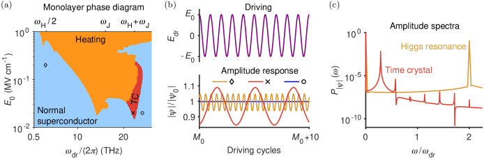
Figure 2: Dynamical phases of a light-driven monolayer cuprate superconductor. (a) Dynamical phase diagram of a monolayer cuprate continuously driven by an electric field with frequency $\omega_{\mathrm{dr}}$ and effective field strength $E_{0}$ at $T=0$. The time crystalline (TC) phase is encoded in red. (b) Driving $E_{\mathrm{dr}}(t)$ and response of the condensate amplitude $|\psi|/|\psi_{0}|(t)$ for the Higgs resonance at $\omega_{\mathrm{dr}}=\omega_{\mathrm{H}}/2$ (diamond), the time crystal (cross), and an off-resonantly driven superconductor (circle). The driving parameters are indicated by the symbols in (a). (c) Power spectra of the condensate amplitude, corresponding to the trajectories of the Higgs resonance and the time crystal presented in (b). The parameters for the monolayer system are the same as in Fig. 1.

We solve the equations of motion for $\psi_{\mathbf{r}}(t)$ and $\mathbf{A}_{\mathbf{r}}(t)$ obtained from the Hamiltonian numerically, employing Heun’s method with an integration step size $\Delta t=1.6~{}\mathrm{as}$. Thermal fluctuations are included by adding dissipation and Langevin noise to the equations of motion for both fields. For example, the time evolution of the superconducting field is given by

$$\partial_{t}\pi_{\mathbf{r}}=-\frac{\partial\mathcal{H}}{\partial\psi_{\mathbf{r}}}-\gamma\pi_{\mathbf{r}}+\xi_{\mathbf{r}},$$ (5)

where $\gamma$ is a damping constant and $\xi_{\mathbf{r}}$ represents white Gaussian noise with zero mean, see Table 1 for noise correlations. We note that the inclusion of in-plane dynamics and arbitrarily strong amplitude fluctuations constitutes a qualitative advance of previous descriptions, such as 1D sine-Gordon models [40, 41].

We determine the response of the superconductor to periodic driving of the electric field along the $c$-axis. The external drive $E_{\mathrm{dr}}(t)$ has the frequency $\omega_{\mathrm{dr}}$ and the effective field strength $E_{0}$. We consider the long-wavelength limit such that the external drive is assumed to be homogeneous in the bulk of the sample. Thus, the time evolution of $E_{z,\mathbf{r}}(t)$ reads

$$\partial_{t}{E}_{z,\mathbf{r}}=\frac{d_{c}}{d_{n}\epsilon_{n}\epsilon_{0}}\frac{\partial\mathcal{H}}{\partial A_{z,\mathbf{r}}}-\gamma E_{z,\mathbf{r}}+\eta_{z,\mathbf{r}}+\frac{\partial_{t}{E}_{\mathrm{dr}}}{\epsilon_{n}},$$ (6)

where $\eta_{z,\mathbf{r}}$ is white Gaussian noise with zero mean. The equations of motion for $E_{x,\mathbf{r}}(t)$ and $E_{y,\mathbf{r}}(t)$ are analogous to Eq. (6), except for the driving term. We characterise the response by evaluating the sample averages of the condensate amplitude $|\psi(t)|$ and the supercurrent density $J(t)$, see also Appendix B.

By applying the optical driving as described, we obtain the full dynamical phase diagram due to the direct coupling of the electromagnetic field to the superconducting order parameter. We note that resonant optical driving of phonon modes has been utilised and discussed in Refs. [1, 2, 3, 40, 41, 42]. Here, we ignore the phononic resonances, so that our predictions are valid away from these resonances. A combined description will be given elsewhere.

III Two-mode model

Before we present the full numerical simulation, we identify the main resonant phenomena of the system. We consider the zero-temperature limit, where the in-plane dynamics can be neglected and the model simplifies to a 1D chain along the $c$-axis. Furthermore, we restrict ourselves to weak driving and a monolayer structure with $t_{s}=t_{w}\equiv t_{\mathrm{J}}$ and $d_{s}=d_{w}\equiv d$. For periodic boundary conditions, the time evolution then reduces to two coupled equations of motion. Keeping only linear terms except for the lowest order coupling between the Higgs field and the unitless vector potential, we find

$$\partial_{t}^{2}a+\gamma\partial_{t}a+\omega_{\mathrm{J}}^{2}a+2\omega_{\mathrm{J}}^{2}ah \approx j_{\mathrm{dr}},$$ (7)

$$\partial_{t}^{2}h+\gamma\partial_{t}h+\omega_{\mathrm{H}}^{2}h+\alpha\omega_{\mathrm{J}}^{2}a^{2} \approx 0,$$ (8)

where $h=(\psi-\psi_{0})/\psi_{0}$ is the Higgs field with $\psi_{0}$ being the equilibrium condensate amplitude, $\gamma$ is the damping constant, and $\alpha$ is the capacitive coupling constant of the junction. Note that the unitless vector potential $a$ equals the phase difference between adjacent planes in this setting. The external drive appears through the current $j_{\mathrm{dr}}$. The Higgs and plasma frequencies are $\omega_{\mathrm{H}}=\sqrt{2\mu/K\hbar^{2}}$ and $\omega_{\mathrm{J}}=\sqrt{t_{\mathrm{J}}/\alpha K\hbar^{2}}$, respectively.

The main finding of this work is the emergence of a time crystalline phase by driving at the sum of the Higgs and plasma frequencies, $\omega_{\mathrm{dr}}=\omega_{\mathrm{J}}+\omega_{\mathrm{H}}$. A cubic interaction process, visualised in Fig. 1(d), allows for simultaneous resonant driving of both the Higgs and the plasma modes [43].

In addition to the sum resonance, we identify various other resonances from the simplified equations of motion. For a response of the vector potential at the driving frequency, i.e., $a=a_{1}\mathrm{cos}(\omega_{\mathrm{dr}}t)$, Eq. (8) simplifies to a forced oscillator with a resonance at $\omega_{\mathrm{dr}}=\omega_{\mathrm{H}}/2$. This recovers the sub-gap Higgs resonance [22]. The sub-gap resonance and the sum resonance originate from the same cubic coupling term $\sim a^{2}h$, as illustrated in Figs. 1(c) and 1(d). Next, we consider the range of driving frequencies where the Higgs field exhibits a second-harmonic response, that is, the external drive induces Higgs oscillations of the form $h=h_{0}+h_{1}\mathrm{cos}(2\omega_{\mathrm{dr}}t)$ through the $a^{2}$ term in Eq. (8). For small driving amplitudes, the $ah$ term in Eq. (7) can be neglected so that the equation reduces to a forced oscillator with a resonance at $\omega_{\mathrm{dr}}=\omega_{\mathrm{J}}$. However, the response is modified once the coupling to the Higgs field becomes significant. Then, Eq. (7) approaches a parametrically driven oscillator. The parametric resonances emerge at $\omega_{\mathrm{dr}}=\omega_{\mathrm{J}}/k$, where $k\in\mathbb{N}$.

IV Dynamical phase diagram

We now present our numerical results in two steps. Firstly, we verify our analytical predictions for the resonances and, in particular, the Higgs time crystal by mapping out the dynamical phase diagrams of mono- and bilayer cuprate superconductors at zero temperature. We will show how the sum resonance is modified in a bilayer system, which has two plasma modes. Secondly, we test the robustness of this phase against thermal fluctuations using finite-temperature simulations.

IV.1 Monolayer cuprate superconductor

Here, we consider a monolayer cuprate with $\omega_{\mathrm{H}}/2\pi\approx 6.3~{}\mathrm{THz}$, $\omega_{\mathrm{J}}/2\pi\approx 16.0~{}\mathrm{THz}$, $\gamma/2\pi=0.5~{}\mathrm{THz}$, and $\alpha=0.33$, see Table 1 for full parameter set. The system is continuously driven at various amplitudes and frequencies in the terahertz regime. In each realisation, the drive is applied for 20 ps and the relevant frequency spectra are computed using the final 10 ps, which amounts to $5<M_{\mathrm{tot}}<300$ driving cycles in the frequency range of interest. The dynamical phase diagram in Fig. 2(a) is mapped out by analysing the normalised power spectra of $|\psi(t)|$ and $J(t)$ defined as $P_{f}(\omega)=\langle f(\omega)f(-\omega)\rangle$, where $\int P_{f}(\omega)d\omega=1$, $f(\omega)=1/\sqrt{T_{s}}\int dt^{\prime}\mathrm{exp}(-\mathrm{i}\omega t^{\prime})f(t^{\prime})$, and $T_{s}=10$ ps is the sampling interval. Specifically, we obtain the spectral entropy for the dynamics of the condensate amplitude, $\mathcal{S}_{|\psi|}=-\int d\omega P_{|\psi|}(\omega)\mathrm{ln}P_{|\psi|}(\omega)$.

The heating regime, which is characterised by a strong depletion of the condensate, is identified based on the threshold $\mathcal{S}_{|\psi|}>2.2\times 10^{-2}$. It indicates the appearance of resonant phases associated with the Higgs and plasma excitations. We note that the two dominant heating tongues are weakly red-detuned from the expected resonance frequencies $\omega_{\mathrm{H}}/2$ and $\omega_{\mathrm{J}}$, respectively. Such a renormalisation of the fundamental frequencies is inherent to strongly driven non-linear systems [44]. This effect is further amplified by the damping terms present in our model. We identify the small tongue at $\omega_{\mathrm{dr}}/2\pi\approx 4.8$ THz as the third order parametric resonance of the Josephson plasma mode around $\omega_{\mathrm{J}}/3$.

For intermediate driving intensity, we observe several dynamical regimes due to resonances. The resonance with the lowest frequency is the Higgs resonance at $\omega_{\mathrm{dr}}=\omega_{\mathrm{H}}/2$. In general, resonant excitation of the Higgs mode is marked by strong modulation of the condensate amplitude as exemplified in Fig. 2(b). Moreover, the Higgs resonance exhibits a commensurate and superharmonic response of $|\psi(t)|$ with respect to the driving $E_{\mathrm{dr}}(t)$ as seen from the closed trajectory in Fig. 1(c) and the sharp peak at $2\omega_{\mathrm{dr}}$ of the condensate amplitude spectrum in Fig. 2(c). We emphasise that driving away from any noticeable resonance, indicated as the blue regime in Fig. 2(a), induces only a single sharp peak in the supercurrent spectrum, namely at the driving frequency. The condensate amplitude oscillates at twice the driving frequency in the blue regime. This also applies to the regime near the Josephson plasma resonance at $\omega_{\mathrm{dr}}=\omega_{\mathrm{J}}$, where the system responds with strong oscillations of the supercurrent.

The red regime in Fig. 2(a), identified via the condition $10^{-4}<\mathcal{S}_{|\psi|}<2.2\times 10^{-2}$, is the Higgs time crystal introduced earlier. We emphasise that its resonance condition $\omega_{\mathrm{dr}}=\omega_{\mathrm{J}}+\omega_{\mathrm{H}}$ differs from the sub-gap frequencies $\omega_{\mathrm{dr}}\lesssim\omega_{\mathrm{H}}/2$ used in standard Higgs spectroscopy. The sum resonance simultaneously couples to the Higgs and plasma resonances as evident from the exemplary mean-field trajectory in Fig. 1(d), where the amplitude oscillation is accompanied by a strong oscillation of the phase difference between the junctions. Despite a smaller driving amplitude $E_{0}$, the plasma mode is excited with larger amplitude than for the Higgs resonance. The strong activation of the plasma mode results in a partial depletion of the condensate as visible in Fig. 2(b), where the time average of the oscillatory motion of the condensate amplitude is below 1. The key feature of the novel phase is the subharmonic response of the condensate amplitude as $|\psi(t)|$ oscillates at $\omega_{\mathrm{H}}$ when the superconductor is driven at $\omega_{\mathrm{dr}}=\omega_{\mathrm{J}}+\omega_{\mathrm{H}}$. This phenomenon is highlighted in Fig. 2(b) and in the strong subharmonic peak in the power spectrum of $|\psi(t)|$ shown in Fig. 2(c). The other dynamical phases respect the time-translation symmetry imposed by the external drive as evidenced by Figs. 2(b) and 2(c).

The subharmonic collective motion is one of the defining features of a time crystal. In addition to being subharmonic, the response of the time crystalline state is also incommensurate to the external driving. That is, the phase-space trajectory traces an open loop for any number of driving cycles, see also Fig. 1(d). Therefore, and more specifically, the state that we propose to create is an incommensurate time crystal in high-$T_{c}$ superconductors. We will confirm its robustness against perturbations of the drive and thermal fluctuations for the bilayer case. We note that the subharmonic response can be expected to be rigid as it emerges for a broad regime of driving parameters rather than a fine-tuned point in the dynamical phase diagram. In addition, our finite-temperature calculations with a large number of lattice sites will highlight the many-body nature of the Higgs time crystal.

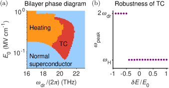
Figure 3: Higgs time crystal in a light-driven bilayer cuprate superconductor. (a) Dynamical phase diagram of a bilayer cuprate continuously driven by an electric field with frequency $\omega_{\mathrm{dr}}$ and effective field strength $E_{0}$ at $T=0$. (b) Robustness of the time crystal (TC) against perturbations of the drive as described in the text. Values of the dominant amplitude frequency $\omega_{\mathrm{peak}}$ close to $\omega_{\mathrm{H}}$ indicate a subharmonic response, whereas maxima at $2\omega_{\mathrm{dr}}$ mark a normal response. The bilayer system has the Higgs frequency $\omega_{\mathrm{H}}/2\pi\approx 6.3$ THz and the two longitudinal Josephson plasma frequencies $\omega_{\mathrm{J}1}/2\pi\approx 2.0~{}\mathrm{THz}$ and $\omega_{\mathrm{J}2}/2\pi\approx 14.3~{}\mathrm{THz}$ at $T=0$, see Table 1 for full parameter set.

IV.2 Bilayer superconductor

We now focus on bilayer cuprates. Due to the staggered tunneling coefficients $t_{s}$ and $t_{w}$ along the $c$-axis, the system has two fundamental longitudinal plasma excitations with frequencies $\omega_{\mathrm{J1}}$ and $\omega_{\mathrm{J2}}$. The dynamical phase diagram at zero temperature in Fig. 3(a) displays a regime, in which a Higgs time crystal is induced by optical driving at a sum resonance. Here, the resonance condition is $\omega_{\mathrm{dr}}=\omega_{\mathrm{H}}+\omega_{\mathrm{J2}}$, so it is the sum of the Higgs frequency and the upper plasma frequency.

First, we examine how perturbing the optical drive itself affects the subharmonic response. To excite the sum resonance, we initially drive the bilayer superconductor with $E_{0}=0.1~{}\mathrm{MV\,cm^{-1}}$ and $\omega_{\mathrm{dr}}/2\pi=21~{}\mathrm{THz}$. At some instant of time $t_{0}$, the driving is altered so that the oscillation amplitude of the field strength depends on its sign for $t>t_{0}$:

$$E_{\mathrm{dr}}(t)=\begin{cases}E_{0}\mathrm{cos}(\omega_{\mathrm{dr}}t)&\mathrm{for}~{}\mathrm{cos}(\omega_{\mathrm{dr}}t)\geq 0,\\ (E_{0}+\delta E)\,\mathrm{cos}(\omega_{\mathrm{dr}}t)&\mathrm{for}~{}\mathrm{cos}(\omega_{\mathrm{dr}}t)<0.\end{cases}$$ (9)

After allowing the system to relax to a steady state, we take the power spectrum of the condensate amplitude and determine the dominant frequency $\omega_{\mathrm{peak}}$. The robustness of the subharmonic response is demonstrated by Fig. 3(b), where perturbations of the driving amplitude between $\delta E/E_{0}=-0.4$ and $\delta E/E_{0}=1$ do not destroy the sum resonance. We have also verified the persistence of the subharmonic response for $10^{5}$ cycles of continuous driving at $T=0$ [43]. Because of experimental and numerical limitations in accessible timescales ($\sim 10^{2}$ driving cycles for our finite-temperature calculations), we will not distinguish here between a ‘true’ time crystal and a slowly decaying time crystal [14, 13].

Figure 4: Higgs time crystal at non-zero temperatures. (a) Comparison between the power spectra of the condensate amplitude at $T=3~{}\mathrm{K}~{}\sim 0.1\,T_{c}$ for $E_{0}=0.2~{}\mathrm{MV\,cm^{-1}}$ and different driving frequencies indicated in the legend. The time crystalline state at $\omega_{\mathrm{dr}}/2\pi=22.4~{}\mathrm{THz}$ is demonstrated by the strongly enhanced subharmonic peak at $\omega_{\mathrm{H}}$. (b) Power spectra of the supercurrent density for the same parameters as in (a). The time crystalline state creates strongly enhanced side peaks at $\omega_{\mathrm{dr}}\pm\omega_{\mathrm{H}}$. (c) Time crystalline fraction $P_{J}(\omega_{\mathrm{dr}}+\omega_{\mathrm{H}})$ in a section of the dynamical phase diagram at $T=3~{}\mathrm{K}~{}\sim 0.1\,T_{c}$, containing the time crystalline phase. (d) Temperature dependence of the optimal time crystalline fraction for a bilayer cuprate superconductor, rescaled by its value at $T=0$. The optimal crystalline fraction at a given temperature corresponds to the maximum value of $P_{J}(\omega_{\mathrm{dr}}+\omega_{\mathrm{H}})$ in the relevant section of the dynamical phase diagram, as exemplified in (c). The error bars in (d) arise from the standard errors of Lorentzian fits to the blue-detuned side peaks. The parameters for the bilayer system are the same as in Fig. 3. The resonance frequencies are shifted at finite temperature.

We note that the time crystalline response is stabilised by the non-linear coupling between the Higgs and plasma modes, which further highlights the collective nature of the Higgs time crystal. Furthermore, the amplitudes of the oscillations are saturated by non-linear processes in the system, see Ref. [45] for example, while the dissipative coupling to the environment limits heating.

Next, we demonstrate the robustness of the Higgs time crystal against thermal fluctuations modelled as Langevin noise in the dynamics of the fields. These fluctuations are a natural test for the rigidity of the subharmonic response against temporal perturbations [13]. When considering thermal fluctuations, we include the in-plane dynamics of the fields in a full 3D simulation. The complete parameter set is summarised in Table 1, implying the Higgs frequency $\omega_{\mathrm{H}}/2\pi\approx 6.3~{}\mathrm{THz}$ and the two longitudinal Josephson plasma frequencies $\omega_{\mathrm{J}1}/2\pi\approx 2.0~{}\mathrm{THz}$ and $\omega_{\mathrm{J}2}/2\pi\approx 14.3~{}\mathrm{THz}$ at $T=0$. For simplicity, we keep the chemical potential fixed in the following finite-temperature calculations, $\mu(T)\equiv\mu$. We choose the parameters within the CuO₂ planes to yield a critical temperature of $T_{c}\sim 30~{}\mathrm{K}$. We find that a discretisation of $48\times 48\times 4$ lattice sites with periodic boundaries is sufficient to obtain fully converged results with respect to the system size. Note that both the Higgs and Josephson plasma frequencies are renormalised at finite temperature [43].

Examples of the power spectra of the condensate amplitude and the supercurrent density at $T=3~{}\mathrm{K}$ are shown in Figs. 4(a) and 4(b), respectively. When the sum resonance is driven, the condensate amplitude exhibits strong subharmonic modulation as evidenced by a sharp peak in the amplitude spectrum in Fig. 4(a). Moreover, we observe in Fig. 4(a) how the modulation of the condensate amplitude is suppressed as the driving frequency is tuned away from the resonance frequency. As shown in Fig. 4(b), we identify an experimentally relevant signature of the superconducting time crystalline phase, which is the appearance of two side peaks at $\omega_{\mathrm{dr}}\pm\omega_{\mathrm{H}}$ in the power spectrum of the supercurrent density. The side peaks vanish as the driving frequency is tuned away from the resonance frequency. Coherent dynamics of supercurrents can be experimentally probed using second-harmonic measurements [46, 47].

To quantify the time crystalline fraction, we use the height of the blue-detuned side peak in the power spectrum of the supercurrent density, $P_{J}(\omega_{\mathrm{dr}}+\omega_{\mathrm{H}})$. Figure 4(d) displays the temperature dependence of the optimal crystalline fraction for a bilayer cuprate, normalised to the optimal time crystalline fraction at $T=0$. The optimal driving parameters at each temperature were inferred from coarse scans such as that in Fig. 4(c). As we expect for time crystals under increasingly strong perturbation, the crystalline fraction decreases with temperature. Nevertheless, the subharmonic response is robust against thermal noise for temperatures up to $T=6~{}\mathrm{K}\sim 0.2\,T_{c}$.

V Pulsed excitation of the
Higgs time crystal

While significant progress has been made in generating continuous-wave terahertz sources [48], typical experiments in optically driven superconductors utilise pulsed excitation, as in most pump-probe experiments. We now point out that the time crystalline phase can be detected when the system is driven with a short pulse, rather than the steady state discussed so far. We consider a pulsed driving scheme by introducing a Gaussian envelope of the periodic driving, that is, $E_{\mathrm{dr}}(t)=E_{0}\mathrm{cos}(\omega_{\mathrm{dr}}t)\,\mathrm{exp}(-t^{2}/2\sigma^{2})$ with the pulse width $\sigma$. In Fig. 5, we present an example of the dynamical response of the bilayer system under pulsed excitation. The response shown in Fig. 5(b) is approximately the Fourier broadened form of Fig. 4(b). The similarity between the two results suggests that the defining features of the Higgs time crystal of continuously driven superconductors are detectable for pulsed driving protocols with realistic pulse lengths. The response can be clearly distinguished from normal dynamical phases by probing the coherent dynamics of the supercurrent. Thus, the Higgs time crystal predicted here can be observed in current state-of-the-art experiments with optically driven high-$T_{c}$ superconductors.

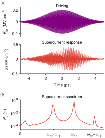
Figure 5: Time crystalline response of a bilayer cuprate superconductor to a driving pulse. (a) Temporal waveform of the pulsed electric field and the induced motion of the supercurrent density shown for one representative trajectory at $T=3~{}\mathrm{K}~{}\sim 0.1\,T_{c}$ with an effective field strength $E_{0}=0.2~{}\mathrm{MV~{}cm}^{-1}$, driving frequency $\omega_{\mathrm{dr}}/2\pi=22.4~{}\mathrm{THz}$, and pulse width $\sigma=2~{}\mathrm{ps}$. (b) Power spectrum of the supercurrent density, measured in the interval between 0 and 2 ps. The parameters for the bilayer system are the same as in Fig. 3.

VI Discussion

In conclusion, we have demonstrated the emergence of a time-crystalline phase in a high-$T_{c}$ superconductor, which is induced by optical driving of a sum resonance of the Higgs mode and a Josephson plasma mode. Using a newly developed lattice gauge simulator, we demonstrate this time crystal for mono- and bilayer cuprates, and show its robustness against thermal fluctuations, for up to $\sim 20\%$ of the critical temperature. As an experimentally accessible signature we observe the emergence of two side peaks at $\omega_{\mathrm{dr}}\pm\omega_{\mathrm{H}}$ in the supercurrent spectra. This signature is also visible in pulsed operation, which mimics realistic experimental conditions.

The emergent time crystalline order that we propose to induce, constitutes a qualitative departure from previous light-induced states in solids, because it is a genuine non-equilibrium state with no equilibrium counterpart. The realisation of such a state expands the scope of the scientific effort to design many-body states by optical driving beyond the paradigm of renormalising equilibrium orders. While even this existing paradigm has been and continues to be thought-provoking and stimulating, the work presented here urges the design and exploration of light-induced non-equilibrium states beyond that framework, and thereby expands the scope of the effort to design quantum matter on demand.

Appendix A Noise correlations

The fluctuation-dissipation theorem requires

$$\langle\mathrm{Re}\{{\xi_{\mathbf{r}}(t)}\}\mathrm{Re}\{{\xi_{\mathbf{r^{\prime}}}(t^{\prime})}\}\rangle =\frac{\gamma K\hbar^{2}k_{\mathrm{B}}T}{V_{0}}\delta_{\mathbf{r}\mathbf{r^{\prime}}}\delta(t-t^{\prime})\,,$$ (10)

$$\langle\mathrm{Im}\{{\xi_{\mathbf{r}}(t)}\}\mathrm{Im}\{{\xi_{\mathbf{r^{\prime}}}(t^{\prime})}\}\rangle =\frac{\gamma K\hbar^{2}k_{\mathrm{B}}T}{V_{0}}\delta_{\mathbf{r}\mathbf{r^{\prime}}}\delta(t-t^{\prime})\,,$$ (11)

$$\langle\mathrm{Re}\{{\xi_{\mathbf{r}}(t)}\}\mathrm{Im}\{{\xi_{\mathbf{r^{\prime}}}(t^{\prime})}\}\rangle =0$$ (12)

for the noise term of the superconducting field, where $V_{0}=d_{ab}^{2}d_{c}$ is the discretisation volume of a single superconducting site. The noise correlations for the electric field are

$$\langle\eta_{x,\mathbf{r}}(t)\eta_{x,\mathbf{r^{\prime}}}(t^{\prime})\rangle =\frac{2\gamma k_{\mathrm{B}}T}{\epsilon_{0}V_{0}}\delta_{\mathbf{r}\mathbf{r^{\prime}}}\delta(t-t^{\prime}),$$ (13)

$$\langle\eta_{y,\mathbf{r}}(t)\eta_{y,\mathbf{r^{\prime}}}(t^{\prime})\rangle =\frac{2\gamma k_{\mathrm{B}}T}{\epsilon_{0}V_{0}}\delta_{\mathbf{r}\mathbf{r^{\prime}}}\delta(t-t^{\prime}),$$ (14)

$$\langle\eta_{z,\mathbf{r}}(t)\eta_{z,\mathbf{r^{\prime}}}(t^{\prime})\rangle =\frac{d_{c}}{d_{n}\epsilon_{n}}\frac{2\gamma k_{\mathrm{B}}T}{\epsilon_{0}V_{0}}\delta_{\mathbf{r}\mathbf{r^{\prime}}}\delta(t-t^{\prime}).$$ (15)

Appendix B Characterisation of the response

We characterise the response of the system to the periodic driving by studying the dynamics of the sample averages of the condensate amplitude and the supercurrent along the $c$-axis. The supercurrent along a single junction in the $c$-direction is given by the Josephson relation

$$J^{z}_{l,m,n}=\frac{4et_{n}d_{c}}{\hbar}\mathrm{Im}\bigl{\{}\psi^{*}_{l,m,n+1}\psi_{l,m,n}e^{ia_{l,m,n}^{z}}\bigr{\}}.$$ (16)

The sample average of the supercurrent density along the $c$-axis can be obtained from

$$J(t)=\frac{d_{s}\overline{J_{s}(t)}+d_{w}\overline{J_{w}(t)}}{d_{s}+d_{w}},$$ (17)

where $\overline{J_{s,w}(t)}$ denotes the spatial average of Josephson currents along either strong or weak junctions. In the case of non-zero temperatures, we average the power spectra $P_{|\psi|}(\omega)$ and $P_{J}(\omega)$ over an ensemble of trajectories. We find that 100 trajectories are enough to obtain convergent results for sampling thermal fluctuations at non-zero temperatures.

Table 1: Model parameters used in the simulations.

	Monolayer	Bilayer
$K~{}(\text{meV}^{-1})$	$\qquad 2.9\times 10^{-5}$	$\qquad 2.9\times 10^{-5}$
$\mu~{}(\text{meV})$	$1.0\times 10^{-2}$	$1.0\times 10^{-2}$
$g~{}(\text{meV \AA}^{3})$	5.0	5.0
$\gamma/2\pi~{}(\text{THz})$	0.5	0.5
$t_{ab}~{}(\text{meV})$	$6.2\times 10^{-1}$	$6.2\times 10^{-1}$
$t_{s}~{}(\text{meV})$	$4.2\times 10^{-2}$	$2.5\times 10^{-2}$
$t_{w}~{}(\text{meV})$		$1.0\times 10^{-3}$
$d_{ab}~{}(\text{\AA})$	15	15
$d_{s}~{}(\text{\AA})$	6	4
$d_{w}~{}(\text{\AA})$		8
$\epsilon_{s}$	1	1
$\epsilon_{w}$		4

Appendix C Model parameters

Table 1 summarises the parameters of our numerical calculations for mono- and bilayer systems, respectively. In both cases, our parameter choice of $\mu$ and $g$ implies an equilibrium condensate density $n_{0}=\mu/g=2\times 10^{21}~{}\mathrm{cm^{-3}}$ at $T=0$. The bilayer system has two longitudinal $c$-axis plasma modes. Their eigenfrequencies are

$$\omega_{\mathrm{J1,J2}}^{2}=\biggl{(}\frac{1}{2}+\alpha_{s}\biggr{)}\Omega_{s}^{2}+\biggl{(}\frac{1}{2}+\alpha_{w}\biggr{)}\Omega_{w}^{2}\mp\sqrt{\biggl{[}\biggl{(}\frac{1}{2}+\alpha_{s}\biggr{)}\Omega_{s}^{2}-\biggl{(}\frac{1}{2}+\alpha_{w}\biggr{)}\Omega_{w}^{2}\biggr{]}^{2}+4\alpha_{s}\alpha_{w}\Omega_{s}^{2}\Omega_{w}^{2}},$$ (18)

as follows from a sine-Gordon analysis at $T=0$ [32, 33]. Here we introduced the bare plasma frequencies of the strong and weak junctions

$$\Omega_{s,w}=\sqrt{\frac{8t_{s,w}n_{0}e^{2}d_{c}d_{s,w}}{\hbar^{2}\epsilon_{s,w}\epsilon_{0}}},$$ (19)

where $d_{c}=(d_{s}+d_{w})/2$. The capacitive coupling constants are given by

$$\alpha_{s,w}=\frac{\epsilon_{s,w}\epsilon_{0}}{8Kn_{0}e^{2}d_{c}d_{s,w}}.$$ (20)

Besides, there is a transverse $c$-axis plasma mode with the eigenfrequency

$$\omega_{\mathrm{T}}^{2}=\frac{1+2\alpha_{s}+2\alpha_{w}}{\alpha_{s}+\alpha_{w}}\,\Bigl{(}\alpha_{s}\Omega_{s}^{2}+\alpha_{w}\Omega_{w}^{2}\Bigr{)}.$$ (21)

We have $\alpha_{s}=0.5$, $\alpha_{w}=1$, $\omega_{\mathrm{J1}}/2\pi\approx 2.0~{}\mathrm{THz}$, $\omega_{\mathrm{J2}}/2\pi\approx 14.3~{}\mathrm{THz}$, and $\omega_{\mathrm{T}}/2\pi\approx 11.8~{}\mathrm{THz}$ for the parameters specified in Table 1. The in-plane plasma frequency amounts to 154 THz.

References

- Fausti et al. [2011] D. Fausti, R. I. Tobey, N. Dean, S. Kaiser, A. Dienst, M. C. Hoffmann, S. Pyon, T. Takayama, H. Takagi, and A. Cavalleri, Light-induced superconductivity in a stripe-ordered cuprate, Science 331, 189 (2011).
- Hu et al. [2014] W. Hu, S. Kaiser, D. Nicoletti, C. R. Hunt, I. Gierz, M. C. Hoffmann, M. Le Tacon, T. Loew, B. Keimer, and A. Cavalleri, Optically enhanced coherent transport in YBa2Cu3O6.5 by ultrafast redistribution of interlayer coupling, Nat. Mater. 13, 705 (2014).
- Cremin et al. [2019] K. A. Cremin, J. Zhang, C. C. Homes, G. D. Gu, Z. Sun, M. M. Fogler, A. J. Millis, D. N. Basov, and R. D. Averitt, Photoenhanced metastable c-axis electrodynamics in stripe-ordered cuprate La1.885Ba0.115CuO4, Proc. Natl. Acad. Sci. USA 116, 19875 (2019).
- Kogar et al. [2019] A. Kogar, A. Zong, P. E. Dolgirev, X. Shen, J. Straquadine, Y.-Q. Bie, X. Wang, T. Rohwer, I.-C. Tung, Y. Yang, R. Li, J. Yang, S. Weathersby, S. Park, M. E. Kozina, E. J. Sie, H. Wen, P. Jarillo-Herrero, I. R. Fisher, X. Wang, and N. Gedik, Light-induced charge density wave in LaTe3, Nat. Phys. 16, 159 (2019).
- Cosme et al. [2018] J. G. Cosme, C. Georges, A. Hemmerich, and L. Mathey, Dynamical control of order in a cavity-BEC system, Phys. Rev. Lett. 121, 153001 (2018).
- Georges et al. [2018] C. Georges, J. G. Cosme, L. Mathey, and A. Hemmerich, Light-induced coherence in an atom-cavity system, Phys. Rev. Lett. 121, 220405 (2018).
- Wilczek [2013] F. Wilczek, Superfluidity and space-time translation symmetry breaking, Phys. Rev. Lett. 111, 250402 (2013).
- Sacha and Zakrzewski [2018] K. Sacha and J. Zakrzewski, Time crystals: a review, Rep. Prog. Phys. 81, 016401 (2018).
- Gambetta et al. [2019] F. M. Gambetta, F. Carollo, M. Marcuzzi, J. P. Garrahan, and I. Lesanovsky, Discrete time crystals in the absence of manifest symmetries or disorder in open quantum systems, Phys. Rev. Lett. 122, 015701 (2019).
- Buca et al. [2019] B. Buca, J. Tindall, and D. Jaksch, Non-stationary coherent quantum many-body dynamics through dissipation, Nat. Commun. 10, 1730 (2019).
- Heugel et al. [2019] T. L. Heugel, M. Oscity, A. Eichler, O. Zilberberg, and R. Chitra, Classical many-body time crystals, Phys. Rev. Lett. 123, 124301 (2019).
- Else et al. [2020] D. V. Else, C. Monroe, C. Nayak, and N. Y. Yao, Discrete time crystals, Annu. Rev. Condens. Matter Phys. 11, 467 (2020).
- Yao et al. [2020] N. Y. Yao, C. Nayak, L. Balents, and M. P. Zaletel, Classical discrete time crystals, Nat. Phys. 16, 438 (2020).
- Choi et al. [2017] S. Choi, J. Choi, R. Landig, G. Kucsko, H. Zhou, J. Isoya, F. Jelezko, S. Onoda, H. Sumiya, V. Khemani, C. von Keyserlingk, N. Y. Yao, E. Demler, and M. D. Lukin, Observation of discrete time-crystalline order in a disordered dipolar many-body system, Nature 543, 221 (2017).
- Zhang et al. [2017] J. Zhang, P. W. Hess, A. Kyprianidis, P. Becker, A. Lee, J. Smith, G. Pagano, I.-D. Potirniche, A. C. Potter, A. Vishwanath, N. Y. Yao, and C. Monroe, Observation of a discrete time crystal, Nature 543, 217 (2017).
- Chew et al. [2020] A. Chew, D. F. Mross, and J. Alicea, Time-crystalline topological superconductors, Phys. Rev. Lett. 124, 096802 (2020).
- Varma [2002] C. M. Varma, Higgs boson in superconductors, J. Low Temp. Phys. 126, 901 (2002).
- Pekker and Varma [2015] D. Pekker and C. Varma, Amplitude/Higgs modes in condensed matter physics, Annu. Rev. Condens. Matter Phys. 6, 269 (2015).
- Matsunaga et al. [2014] R. Matsunaga, N. Tsuji, H. Fujita, A. Sugioka, K. Makise, Y. Uzawa, H. Terai, Z. Wang, H. Aoki, and R. Shimano, Light-induced collective pseudospin precession resonating with Higgs mode in a superconductor, Science 345, 1145 (2014).
- Tsuji and Aoki [2015] N. Tsuji and H. Aoki, Theory of Anderson pseudospin resonance with Higgs mode in superconductors, Phys. Rev. B 92, 064508 (2015).
- Nakamura et al. [2019] S. Nakamura, Y. Iida, Y. Murotani, R. Matsunaga, H. Terai, and R. Shimano, Infrared activation of the Higgs mode by supercurrent injection in superconducting NbN, Phys. Rev. Lett. 122, 257001 (2019).
- Shimano and Tsuji [2020] R. Shimano and N. Tsuji, Higgs mode in superconductors, Annu. Rev. Condens. Matter Phys. 11, 103 (2020).
- Peronaci et al. [2015] F. Peronaci, M. Schiró, and M. Capone, Transient dynamics of -wave superconductors after a sudden excitation, Phys. Rev. Lett. 115, 257001 (2015).
- Katsumi et al. [2018] K. Katsumi, N. Tsuji, Y. I. Hamada, R. Matsunaga, J. Schneeloch, R. D. Zhong, G. D. Gu, H. Aoki, Y. Gallais, and R. Shimano, Higgs mode in the -wave superconductor driven by an intense terahertz pulse, Phys. Rev. Lett. 120, 117001 (2018).
- Buzzi et al. [2019] M. Buzzi, G. Jotzu, A. Cavalleri, J. I. Cirac, E. A. Demler, B. I. Halperin, M. D. Lukin, T. Shi, Y. Wang, and D. Podolsky, Higgs-mediated optical amplification in a non-equilibrium superconductor, arXiv e-prints (2019), arXiv:1908.10879 [cond-mat.supr-con] .
- Chu et al. [2020] H. Chu, M.-J. Kim, K. Katsumi, S. Kovalev, R. D. Dawson, L. Schwarz, N. Yoshikawa, G. Kim, D. Putzky, Z. Z. Li, H. Raffy, S. Germanskiy, J.-C. Deinert, N. Awari, I. Ilyakov, B. Green, M. Chen, M. Bawatna, G. Christiani, G. Logvenov, Y. Gallais, A. V. Boris, B. Keimer, A. P. Schnyder, D. Manske, M. Gensch, Z. Wang, R. Shimano, and S. Kaiser, Phase-resolved Higgs response in superconducting cuprates, Nat. Commun. 11, 1793 (2020).
- Schwarz et al. [2020] L. Schwarz, B. Fauseweh, N. Tsuji, N. Cheng, N. Bittner, H. Krull, M. Berciu, G. S. Uhrig, A. P. Schnyder, S. Kaiser, and D. Manske, Classification and characterization of nonequilibrium Higgs modes in unconventional superconductors, Nat. Commun. 11, 287 (2020).
- Puviani et al. [2020] M. Puviani, L. Schwarz, X.-X. Zhang, S. Kaiser, and D. Manske, Current-assisted Raman activation of the Higgs mode in superconductors, Phys. Rev. B 101, 220507 (2020).
- Yang and Wu [2020] F. Yang and M. W. Wu, Theory of Higgs modes in -wave superconductors, Phys. Rev. B 102, 014511 (2020).
- Yuzbashyan et al. [2006] E. A. Yuzbashyan, O. Tsyplyatyev, and B. L. Altshuler, Relaxation and persistent oscillations of the order parameter in fermionic condensates, Phys. Rev. Lett. 96, 097005 (2006).
- Koyama and Tachiki [1996] T. Koyama and M. Tachiki, I-V characteristics of Josephson-coupled layered superconductors with longitudinal plasma excitations, Phys. Rev. B 54, 16183 (1996).
- van der Marel and Tsvetkov [2001] D. van der Marel and A. A. Tsvetkov, Transverse-optical Josephson plasmons: Equations of motion, Phys. Rev. B 64, 024530 (2001).
- Koyama [2002] T. Koyama, Josephson plasma resonances and optical properties in high- superconductors with alternating junction parameters, J. Phys. Soc. Jpn. 71, 2986 (2002).
- Shibata and Yamada [1998] H. Shibata and T. Yamada, Double josephson plasma resonance in phase , Phys. Rev. Lett. 81, 3519 (1998).
- Dulić et al. [2001] D. Dulić, A. Pimenov, D. van der Marel, D. M. Broun, S. Kamal, W. N. Hardy, A. A. Tsvetkov, I. M. Sutjaha, R. Liang, A. A. Menovsky, A. Loidl, and S. S. Saxena, Observation of the transverse optical plasmon in , Phys. Rev. Lett. 86, 4144 (2001).
- Basov and Timusk [2005] D. N. Basov and T. Timusk, Electrodynamics of high- superconductors, Rev. Mod. Phys. 77, 721 (2005).
- Ginzburg and Landau [1950] V. L. Ginzburg and L. D. Landau, On the theory of superconductivity, Zh. Eksp. Teor. Fiz. 20, 1064 (1950).
- Kogut [1979] J. B. Kogut, An introduction to lattice gauge theory and spin systems, Rev. Mod. Phys. 51, 659 (1979).
- Yee [1966] K. Yee, Numerical solution of initial boundary value problems involving maxwell’s equations in isotropic media, IEEE Trans. Antennas Propag. 14, 302 (1966).
- Denny et al. [2015] S. J. Denny, S. R. Clark, Y. Laplace, A. Cavalleri, and D. Jaksch, Proposed parametric cooling of bilayer cuprate superconductors by terahertz excitation, Phys. Rev. Lett. 114, 137001 (2015).
- Okamoto et al. [2016] J.-i. Okamoto, A. Cavalleri, and L. Mathey, Theory of enhanced interlayer tunneling in optically driven high- superconductors, Phys. Rev. Lett. 117, 227001 (2016).
- Okamoto et al. [2017] J.-i. Okamoto, W. Hu, A. Cavalleri, and L. Mathey, Transiently enhanced interlayer tunneling in optically driven high- superconductors, Phys. Rev. B 96, 144505 (2017).
- [43] See Supplemental Material for a multiple-scale analysis of the sum resonance, rigidity of the Higgs time crystal, conductivity measurements in the time crystalline phase, and information on the thermal phase transition and the temperature dependence of the resonance frequencies.
- Landau and Lifšic [1976] L. D. Landau and E. M. Lifšic, Mechanics, 3rd ed. (Butterworth-Heinemann, Oxford, 1976).
- Nayfeh [1983] A. H. Nayfeh, Combination resonances in the non-linear response of bowed structures to a harmonic excitation, J. Sound Vib. 90, 457 (1983).
- von Hoegen et al. [2018] A. von Hoegen, R. Mankowsky, M. Fechner, M. Först, and A. Cavalleri, Probing the interatomic potential of solids with strong-field nonlinear phononics, Nature 555, 79 (2018).
- von Hoegen et al. [2019] A. von Hoegen, M. Fechner, M. Först, J. Porras, B. Keimer, M. Michael, E. Demler, and A. Cavalleri, Probing coherent charge fluctuations in YBa2Cu3O6+x at wavevectors outside the light cone, arXiv e-prints (2019), arXiv:1911.08284 [cond-mat.supr-con] .
- Welp et al. [2013] U. Welp, K. Kadowaki, and R. Kleiner, Superconducting emitters of THz radiation, Nat. Photon. 7, 702 (2013).