A new 3D model for magnetic particle imaging using realistic magnetic field topologies for algebraic reconstruction

Gaël Bringout1,2, Wolfgang Erb3, Jürgen Frikel4 1 Universität zu Lübeck, Ratzeburger Allee 160, 23562 Lübeck, Germany
2 Physikalisch-Technische Bundesanstalt (PTB), Abbestr. 2-12, 10587 Berlin-Charlottenburg, Germany
3 Università degli Studi di Padova, Via Trieste 63, 35121 Padova, Italy
4 Ostbayerische Technische Hochschule Regensburg, Galgenbergstr. 32, 93053 Regensburg, Germany
gael.bringout@gmail.com, wolfgang.erb@lissajous.it, juergen.frikel@oth-regensburg.de
Abstract

We derive a new 3D model for magnetic particle imaging (MPI) that is able to incorporate realistic magnetic fields in the reconstruction process. In real MPI scanners, the generated magnetic fields have distortions that lead to deformed magnetic low-field volumes (LFV) with the shapes of ellipsoids or bananas instead of ideal field-free points (FFP) or lines (FFL), respectively. Most of the common model-based reconstruction schemes in MPI use however the idealized assumption of an ideal FFP or FFL topology and, thus, generate artifacts in the reconstruction. Our model-based approach is able to deal with these distortions and can generally be applied to dynamic magnetic fields that are approximately parallel to their velocity field. We show how this new 3D model can be discretized and inverted algebraically in order to recover the magnetic particle concentration. To model and describe the magnetic fields, we use decompositions of the fields in spherical harmonics. We complement the description of the new model with several simulations and experiments.

Keywords: Magnetic Particle Imaging (MPI), model-based algebraic reconstruction, description of magnetic fields with spherical harmonics, MPI model for realistic magnetic fields, low-field volume, field-free line, field-free point

1 Introduction

The smart design of magnetic coils for the generation of oscillating magnetic fields is a key challenge in Magnetic Particle Imaging (MPI) [2, 16]. The generated magnetic fields combined with the non-linear magnetization response of the tracer material consisting of superparamagnetic iron oxide nanoparticles (SPIONs) determine the signal acquisition process in MPI and, ultimately, how the distribution of SPIONs can be reconstructed. For this reason an accurate description and analysis of realistic magnetic fields is essential to study modelling and reconstruction in MPI.

Since the first publication in 2005 [6], Magnetic Particle Imaging has undergone major development steps based on a few major designs for the generation of magnetic fields. For two of these topologies, generally referred to as field-free point (FFP) and field-free line (FFL) topology, fully 3D commercial preclinical MPI scanners are available at the present moment that are able to track SPIONs with a high sensitivity and a high temporal resolution. This makes the biomedical imaging modality MPI to a promising tracer-based diagnostic tool, in particulur for blood flow imaging or for quantitative stem cell imaging [19, 22, 24].

In the original scanner design for MPI developed at Philips research (introduced in [6], extended to a full in vivo 3D design in [29]), a static gradient field with a space-homogeneous time-varying drive field is combined in order to magnetize the SPIONs. The two fields are generated in such a way that a moving spot is created in which the resulting magnetic field is low. The center of this low-field spot in which the magnetic field ideally vanishes is called the field-free point (FFP). As soon as the FFP moves over a distribution of SPIONs, the magnetization of the SPIONs starts to flip, inducing a measurable voltage signal in one or several receive coils. From this time-dependent voltage signal the position of the SPIONs can be reconstructed. In the original Philips design, the FFP of the created field moves along a 3D Lissajous trajectory inside a rectangular volume. Later on, also other FFP-trajectories have been introduced in MPI, see [15].

In [28], a second major design principle for magnetic fields was introduced in which the applied magnetic fields ideally vanish along a field-free line (FFL). Compared to the FFP setting, the voltage signal is now created in a much larger low field region along the field-free line, providing a higher sensitivity [28] during the scan. A second main advantage of the FFL topology is the availability of an efficient model-based reconstruction formula based on the inverse Radon transform [18].

For both field topologies, FFP and FFL, models for the reconstruction of the particle density have been derived. However, only in very idealized settings, as for a 1D-FFP along line segments [4, 7, 23] or a non-rotating FFL [2, 5, 18], simple and reliable reconstruction formulas are available. While these simple formulas can be incorporated successfully also in 2D and 3D reconstructions [8, 21, 25], they lead to artifacts once the directions of the magnetic fields are altering quickly, as for instance if the FFP is moving on a 3D Lissajous curve. This discrepancy is due to limited possibilities to describe the magnetization behavior of nonuniform anisotropic SPIONs correctly if the external magnetic fields are changing rapidly their orientation. In this case, complex numerical simulations of the Fokker-Planck equations for coupled Brown/Néel rotations are necessary to describe the imaging properly, see [12, 14, 27].

Moreover, in practice, real magnetic fields involved in the generation of a FFP or a FFL contain distortions. In particular in the FFL setting, the low-field volume (LFV) of the field has more the appearance of a slightly bended banana than that of a stright line [2, 5]. While using the inverse Radon transform for signals created by an ideal FFL yields a reasonable recovery of the particle concentration, this is no longer the case for realistic magnetic fields. In this case, the given distortions lead to serious artifacts in the reconstruction, in particular at the boundary of the field of view (as illustrated in the Tables 4 and 5 below). A further problem arises from the particular dynamic generation of the FFL. In order to accelerate the signal acquisition process, the FFL is continuously rotated with a frequency frotsubscript𝑓rotf_{\mathrm{rot}} [17]. As the classical filtered backprojection is computed on a rectangular grid in Radon space, the regridding from the rotated Radon information causes additional artifacts in the reconstruction.

The goal of this article is to introduce and study a new 3D model for MPI that is able to incorporate realistic magnetic fields, and to provide a simple reconstruction algorithm at the same time. More precisely, for realistic uni-directional time-oscillating magnetic fields we aim at obtaining a model-based reconstruction formula that generalizes the known FFL and 1D-FFP formulas in MPI. This new model-based reconstruction reduces artifacts generated by distortions and the rotation dynamics of the magnetic fields and allows us to calculate the particle concentration in an efficient way based on an algebraic method.

To this end, we introduce a family of magnetic fields in which the field is parallel to its own velocity field. For this family of fields, the direction of the field does not change over time, allowing to substitute the general MPI imaging equation with a simpler 3D integral equation that can be discretized in an efficient way. In the mathematical formulation we use spherical harmonic expansions of magnetic fields (as introduced in [2, 3]) and, as important examples, we show that this modelling framework includes classical (ideal) models, like the 1D-FFP along a straight line [4, 23] and the ideal FFL [18]. In particular, we show that this formulation offers enough flexibility to model realistic magnetic fields, e.g. in a FFL-type setting, by including higher order harmonics into the expansion. The coefficients of the higher order harmonics can be measured in a calibration procedure providing a realistic MPI model for a particular scanner. In this context, our MPI modelling framework can be interpreted as a hybrid between model-based and measurement-based approach in which the parameters of the magnetic fields are determined in a preliminary step.

1.1 Contributions

  • (i)

    We introduce a new modelling framework in MPI based on the expansion of magnetic fields in spherical harmonics and homogeneous harmonic polynomials, and we show how ideal and realistic magnetic field topologies in MPI can be modeled within this framework.

  • (ii)

    We state a new 3D3𝐷3D MPI model for magnetic fields in which the velocity and the acceleration field are parallel. Applied to ideal cases, this general model explains the standard 1D-FFP and FFL reconstruction formulas.

  • (iii)

    We use this new model to obtain a model-based reconstruction that is able to handle realistic magnetic fields in FFL-type imaging. This new model-based approach is able to significantly reduce artifacts in the reconstruction caused by idealized assumptions on the magnetic fields.

  • (iv)

    We give a numerical implementation of this reconstruction scheme and provide several simulations and experiments complementing our results.

1.2 Outline of the paper

We continue this introductury part by giving a brief overview about the general imaging concepts in MPI (Section 2). We further give a mathematical description of important ideal and realistic magnetic field topologies encountered in MPI (Section 3). The new model used for the algebraic reconstruction of the particle concentration with realistic field topologies is derived in Section 4. It is formulated in terms of magnetic fields that are parallel to their velocity field. This familiy of fields contains all relevant ideal and realistic topologies in the considered FFL-type imaging scenario. The numerical details to obtain a discrete system matrix from the given continuous model, including approximation and discretization techniques, are provided in Section 5. Finally, the experiments in Section 6 show that the new algebraic reconstruction approach based on a model with realistic magnetic fields is very promising and outperforms a direct reconstruction using a filtered back projection. We conclude this article in Section 7.

2 Principles of MPI signal generation

2.1 General imaging model in MPI

The basic concept of Magnetic Particle Imaging (MPI) is to recover a density c(𝒓)𝑐𝒓c(\boldsymbol{r}) of SPIONs from their non-linear magnetization in an applied time-varying magnetic field 𝑩(𝒓,t)𝑩𝒓𝑡\boldsymbol{B}(\boldsymbol{r},t). In an MPI scanner, this change in the magnetization of the superparamagnetic particles is measuered in terms of voltage signals induced in one or several receive coils. Neglecting particle-particle interactions, the corresponding general imaging equation is determined by Faraday’s law of induction and is given as ([16, Eq. (2.36)])

uν(t)=μ0ddtΩϱν(𝒓), ¯𝑴(𝑩(𝒓,t))c(𝒓)d𝒓.subscript𝑢𝜈𝑡subscript𝜇0dd𝑡subscriptΩsubscriptbold-italic-ϱ𝜈𝒓 ¯𝑴𝑩𝒓𝑡𝑐𝒓differential-d𝒓u_{\nu}(t)=-\mu_{0}{\frac{\mathrm{d}}{\mathrm{d}t}}\int_{\Omega}\left\langle\boldsymbol{\varrho}_{\nu}(\boldsymbol{r}),\hbox to0.0pt{\hskip 2.89581pt\leavevmode\hbox{\set@color$\overline{\hbox{}}$}\hss}{\leavevmode\hbox{\set@color$\boldsymbol{M}$}}(\boldsymbol{B}(\boldsymbol{r},t))\right\rangle\,c(\boldsymbol{r})\,\mathrm{d}\boldsymbol{r}. (1)

Here, uν(t)subscript𝑢𝜈𝑡u_{\nu}(t) denotes the induced voltage in the receive coil ν{1,,V}𝜈1𝑉\nu\in\{1,\ldots,V\} and ϱν(𝒓)subscriptbold-italic-ϱ𝜈𝒓\boldsymbol{\varrho}_{\nu}(\boldsymbol{r}) the sensitivity vector of the receive coil ν𝜈\nu pointing in direction of the central axis of the coil. The function c(𝒓)𝑐𝒓c(\boldsymbol{r}) denotes the particle density at the point 𝒓𝒓\boldsymbol{r} in the domain Ω3Ωsuperscript3\Omega\subset\mathbb{R}^{3}. Finally, ¯¯\overline{\hbox{}}𝑴𝑴\boldsymbol{M} describes the magnetization response of a single mean SPION depending on the applied magnetic field 𝑩(𝒓,t)𝑩𝒓𝑡\boldsymbol{B}(\boldsymbol{r},t).

This equation describes a general imaging situation in MPI. For a particular measurement setup the sensitivities ϱνsubscriptbold-italic-ϱ𝜈\boldsymbol{\varrho}_{\nu}, the magnetization response function ¯¯\overline{\hbox{}}𝑴𝑴\boldsymbol{M} and the employed magnetic fields 𝑩(𝒓,t)𝑩𝒓𝑡\boldsymbol{B}(\boldsymbol{r},t) have to be modelled or specified.

2.2 Magnetic fields and magnetization

The magnetization ¯¯\overline{\hbox{}}𝑴𝑴\boldsymbol{M} of a single SPION is aligned along the direction of the applied magnetic field 𝑩(𝒓,t)𝑩𝒓𝑡\boldsymbol{B}(\boldsymbol{r},t) and can be written as

 ¯𝑴(𝑩(𝒓,t))= ¯m(|𝑩(𝒓,t)|)𝑩(𝒓,t)|𝑩(𝒓,t)|, ¯𝑴𝑩𝒓𝑡 ¯m𝑩𝒓𝑡𝑩𝒓𝑡𝑩𝒓𝑡\hbox to0.0pt{\hskip 2.89581pt\leavevmode\hbox{\set@color$\overline{\hbox{}}$}\hss}{\leavevmode\hbox{\set@color$\boldsymbol{M}$}}(\boldsymbol{B}(\boldsymbol{r},t))=\hbox to0.0pt{\hskip 1.66667pt\leavevmode\hbox{\set@color$\overline{\hbox{}}$}\hss}{\leavevmode\hbox{\set@color$\mathrm{m}$}}(|\boldsymbol{B}(\boldsymbol{r},t)|)\ \frac{\boldsymbol{B}(\boldsymbol{r},t)}{|\boldsymbol{B}(\boldsymbol{r},t)|}, (2)

A classical way to describe the modulus ¯¯\overline{\hbox{}}mm\mathrm{m} of the magnetization is the Langevin theory of paramagnetism. In this theory the mean modulus ¯¯\overline{\hbox{}}mm\mathrm{m} is modeled as

 ¯m(|𝑩|)=m0L(λ|𝑩|), ¯m𝑩subscript𝑚0𝐿𝜆𝑩\hbox to0.0pt{\hskip 1.66667pt\leavevmode\hbox{\set@color$\overline{\hbox{}}$}\hss}{\leavevmode\hbox{\set@color$\mathrm{m}$}}(|\boldsymbol{B}|)=m_{0}L(\lambda|\boldsymbol{B}|), (3)

with the Langevin function L(x)𝐿𝑥L(x) and the constant λ𝜆\lambda given by

L(x)=cothx1xandλ=μ0m0kBT.formulae-sequence𝐿𝑥hyperbolic-cotangent𝑥1𝑥and𝜆subscript𝜇0subscript𝑚0subscript𝑘B𝑇L(x)=\coth x-\frac{1}{x}\quad\text{and}\quad\lambda=\frac{\mu_{0}m_{0}}{k_{\mathrm{B}}T}.

Here, m0subscript𝑚0m_{0} denotes the magnetic moment of a single SPION, μ0subscript𝜇0\mu_{0} the permeability in free space, kBsubscript𝑘Bk_{\mathrm{B}} the Boltzmann constant and T𝑇T the temperature. The Langevin function L(x)𝐿𝑥L(x) is a point symmetric function with respect to the origin and converges for x±𝑥plus-or-minusx\to\pm\infty to limx±L(x)=±1subscript𝑥plus-or-minus𝐿𝑥plus-or-minus1\lim_{x\to\pm\infty}L(x)=\pm 1. Its derivative is given by

L(x)={13,x=0,1x21sinh2(x),x0.superscript𝐿𝑥cases13𝑥01superscript𝑥21superscript2𝑥𝑥0L^{\prime}(x)=\begin{cases}\displaystyle\frac{1}{3},&x=0,\\[4.30554pt] \frac{1}{x^{2}}-\frac{1}{\sinh^{2}(x)},&x\neq 0.\end{cases} (4)

For the modulus ¯¯\overline{\hbox{}}mm\mathrm{m}, we therefore get  ¯m(|𝑩|)=m0λL(λ|𝑩|)superscript ¯m𝑩subscript𝑚0𝜆superscript𝐿𝜆𝑩\hbox to0.0pt{\hskip 1.66667pt\leavevmode\hbox{\set@color$\overline{\hbox{}}$}\hss}{\leavevmode\hbox{\set@color$\mathrm{m}$}}^{\prime}(|\boldsymbol{B}|)=m_{0}\lambda L^{\prime}(\lambda|\boldsymbol{B}|) and asymptotically lim|𝑩| ¯m(|𝑩|)=m0subscript𝑩 ¯m𝑩subscript𝑚0\lim_{|\boldsymbol{B}|\to\infty}\hbox to0.0pt{\hskip 1.66667pt\leavevmode\hbox{\set@color$\overline{\hbox{}}$}\hss}{\leavevmode\hbox{\set@color$\mathrm{m}$}}(|\boldsymbol{B}|)=m_{0}. For a large vector field strength |𝑩|𝑩|\boldsymbol{B}| the saturation of the magnetization is therefore described by m0subscript𝑚0m_{0}. The derivative  ¯m(0)=m0λ/3superscript ¯m0subscript𝑚0𝜆3\hbox to0.0pt{\hskip 1.66667pt\leavevmode\hbox{\set@color$\overline{\hbox{}}$}\hss}{\leavevmode\hbox{\set@color$\mathrm{m}$}}^{\prime}(0)=m_{0}\lambda/3 is a measure for the magnetic susceptibility of a particle.

2.3 Extension of curl- and divergence-free magnetic fields

In a volume with no magnetic field source and constant permeability μ0subscript𝜇0\mu_{0}, as for instance in the interior of a cylindrical coil, a magnetic field 𝑩𝑩\boldsymbol{B} can be regarded both as a divergence-free and a curl-free vector field (see [2, Section 2.1.2] or [10, Section 5.4]), i.e. it satisfies the two equations

𝑩=0and×𝑩=𝟎.formulae-sequence𝑩0and𝑩0\nabla\cdot\boldsymbol{B}=0\quad\text{and}\quad\nabla\times\boldsymbol{B}=\boldsymbol{0}.

The second identity implies that 𝑩𝑩\boldsymbol{B} is locally a conservative vector field and can be written as the gradient 𝑩=φ𝑩𝑩subscript𝜑𝑩\boldsymbol{B}=\nabla\varphi_{\boldsymbol{B}} of a potential function φ𝑩subscript𝜑𝑩\varphi_{\boldsymbol{B}}. The fact that 𝑩𝑩\boldsymbol{B} is divergence-free then implies that φ𝑩subscript𝜑𝑩\varphi_{\boldsymbol{B}} satisfies the Laplace equation Δφ𝑩=0Δsubscript𝜑𝑩0\Delta\varphi_{\boldsymbol{B}}=0. In particular, assuming that the vector field 𝑩𝑩\boldsymbol{B} is sufficiently smooth, the identity Δφ𝑩=0Δsubscript𝜑𝑩0\Delta\varphi_{\boldsymbol{B}}=0 implies that also every component Bjsubscript𝐵𝑗B_{j} of the vector field 𝑩=(B1,B2,B3)𝑩subscript𝐵1subscript𝐵2subscript𝐵3\boldsymbol{B}=(B_{1},B_{2},B_{3}) is a solution of the Laplace equation ΔBj=0Δsubscript𝐵𝑗0\Delta B_{j}=0, j{1,2,3}𝑗123j\in\{1,2,3\}. As proposed in [3], this fact enables us to extend the components Bjsubscript𝐵𝑗B_{j} of the vector field 𝑩𝑩\boldsymbol{B} in terms of spherical harmonics in order to get a compact description of the magnetic fields in MPI.

2.3.1 Homogeneous harmonic polynomials.

A homogeneous polynomial in 3superscript3\mathbb{R}^{3} of degree l0𝑙subscript0l\in\mathbb{N}_{0} is a linear combination of the monomials

xi1yi2zi3,i1+i2+i3=l.superscript𝑥subscript𝑖1superscript𝑦subscript𝑖2superscript𝑧subscript𝑖3subscript𝑖1subscript𝑖2subscript𝑖3𝑙x^{i_{1}}y^{i_{2}}z^{i_{3}},\quad i_{1}+i_{2}+i_{3}=l.

The space 𝒫lsubscript𝒫𝑙\mathcal{P}_{l} of all homogeneous polynomials of degree l𝑙l has the dimension

dim𝒫l=(l+1)(l+2)2.dimensionsubscript𝒫𝑙𝑙1𝑙22\dim\mathcal{P}_{l}=\frac{(l+1)(l+2)}{2}.

Herein, the subspace lsubscript𝑙\mathcal{H}_{l} of homogeneous harmonic polynomials of degree l𝑙l is given by the polynomials p𝒫l𝑝subscript𝒫𝑙p\in\mathcal{P}_{l} satisfying the Laplace equation

Δp(x,y,z)=0.Δ𝑝𝑥𝑦𝑧0\Delta p(x,y,z)=0.

In this way, the spaces lsubscript𝑙\mathcal{H}_{l} are natural candidates to approximate and expand the components Bisubscript𝐵𝑖B_{i} of the magnetic field 𝑩𝑩\boldsymbol{B}. The dimension of the harmonic spaces lsubscript𝑙\mathcal{H}_{l} is given by diml=dim𝒫ldim𝒫l2=2l+1dimensionsubscript𝑙dimensionsubscript𝒫𝑙dimensionsubscript𝒫𝑙22𝑙1\dim\mathcal{H}_{l}=\dim\mathcal{P}_{l}-\dim\mathcal{P}_{l-2}=2l+1.

2.3.2 Spherical harmonics.

A homogeneous harmonic polynomial pl𝑝subscript𝑙p\in\mathcal{H}_{l} of degree l0𝑙subscript0l\in\mathbb{N}_{0} can be written in spherical coordinates (r,θ,φ)𝑟𝜃𝜑(r,\theta,\varphi) as a linear combination of particular basis functions defined in terms of spherical harmonics. Namely, with the spherical coordinates given by

(x,y,z)=(rsinθcosφ,rsinθsinφ,rcosθ),𝑥𝑦𝑧𝑟𝜃𝜑𝑟𝜃𝜑𝑟𝜃(x,y,z)=(r\sin\theta\cos\varphi,r\sin\theta\sin\varphi,r\cos\theta),

the polynomials

pl,m(r,θ,φ)=rlYl,m(θ,φ),m=l,,l,formulae-sequencesubscript𝑝𝑙𝑚𝑟𝜃𝜑superscript𝑟𝑙subscript𝑌𝑙𝑚𝜃𝜑𝑚𝑙𝑙p_{l,m}(r,\theta,\varphi)=r^{l}Y_{l,m}(\theta,\varphi),\quad m=-l,\ldots,l,

form a basis for the space lsubscript𝑙\mathcal{H}_{l} of harmonic polynomials. Here, Yl,m(θ,φ)subscript𝑌𝑙𝑚𝜃𝜑Y_{l,m}(\theta,\varphi) denote the 2l+12𝑙12l+1 real-valued Schmidt semi-normalized spherical harmonics of degree l𝑙l given by

Yl,m(θ,φ)={2(lm)!(l+m)!Plm(cosθ)cos(mφ)if m{1,,l},Pl0(cosθ)if m=0,2(lm)!(l+m)!Pl|m|(cosθ)sin(|m|φ)if m{1,2,,l},subscript𝑌𝑙𝑚𝜃𝜑cases2𝑙𝑚𝑙𝑚superscriptsubscript𝑃𝑙𝑚𝜃𝑚𝜑if m{1,,l},superscriptsubscript𝑃𝑙0𝜃if m=0,2𝑙𝑚𝑙𝑚superscriptsubscript𝑃𝑙𝑚𝜃𝑚𝜑if m{1,2,,l},Y_{l,m}(\theta,\varphi)=\left\{\begin{array}[]{ll}\textstyle\sqrt{2\frac{(l-m)!}{(l+m)!}}P_{l}^{m}(\cos\theta)\cos(m\varphi)&\text{if $m\in\{1,\ldots,l\}$,}\\ P_{l}^{0}(\cos\theta)&\text{if $m=0$,}\\ \textstyle\sqrt{2\frac{(l-m)!}{(l+m)!}}P_{l}^{|m|}(\cos\theta)\sin(|m|\varphi)&\text{if $m\in\{-1,-2,\ldots,-l\}$,}\end{array}\right.

where Plmsuperscriptsubscript𝑃𝑙𝑚P_{l}^{m}, l,m𝑙𝑚l,m\in\mathbb{N}, 0ml0𝑚𝑙0\leq m\leq l, denote the associated Legendre polynomials given by

Plm(x)=12ll!(1x2)m/2dl+mdxl+m(x21)l.superscriptsubscript𝑃𝑙𝑚𝑥1superscript2𝑙𝑙superscript1superscript𝑥2𝑚2superscriptd𝑙𝑚dsuperscript𝑥𝑙𝑚superscriptsuperscript𝑥21𝑙P_{l}^{m}(x)={\frac{1}{2^{l}l!}}(1-x^{2})^{m/2}\ {\frac{\mathrm{d}^{l+m}}{\mathrm{d}x^{l+m}}}(x^{2}-1)^{l}.

Note that we omit the frequently used Condon-Shortly phase (1)msuperscript1𝑚(-1)^{m} in the definition of Plmsuperscriptsubscript𝑃𝑙𝑚P_{l}^{m} (see [10, Section 3.5]). In Table 1, the spherical harmonics and the corresponding harmonic polynomials up to degree l=2𝑙2l=2 are listed.

Table 1: Spherical harmonics and harmonic homogeneous polynomials of degree l2𝑙2l\leq 2.
Degree l𝑙l Yl,m(θ,φ)subscript𝑌𝑙𝑚𝜃𝜑Y_{l,m}(\theta,\varphi) pl,m(𝒓)subscript𝑝𝑙𝑚𝒓p_{l,m}(\boldsymbol{r})
00 Y0,0(θ,φ)=1subscript𝑌00𝜃𝜑1\begin{array}[]{l}Y_{0,0}(\theta,\varphi)=1\end{array} p0,0(𝒓)=1subscript𝑝00𝒓1\begin{array}[]{l}p_{0,0}(\boldsymbol{r})=1\end{array}
111 Y1,1(θ,φ)=sinθcosφY1,0(θ,φ)=cosθY1,1(θ,φ)=sinθsinφsubscript𝑌11𝜃𝜑𝜃𝜑subscript𝑌10𝜃𝜑𝜃subscript𝑌11𝜃𝜑𝜃𝜑\begin{array}[]{l}Y_{1,1}(\theta,\varphi)=\sin\theta\cos\varphi\\ Y_{1,0}(\theta,\varphi)=\cos\theta\\ Y_{1,-1}(\theta,\varphi)=\sin\theta\sin\varphi\end{array} p1,1(𝒓)=xp1,0(𝒓)=zp1,1(𝒓)=ysubscript𝑝11𝒓𝑥subscript𝑝10𝒓𝑧subscript𝑝11𝒓𝑦\begin{array}[]{l}p_{1,1}(\boldsymbol{r})=x\\ p_{1,0}(\boldsymbol{r})=z\\ p_{1,-1}(\boldsymbol{r})=y\end{array}
222 Y2,2(θ,φ)=32sin2θcos2φY2,1(θ,φ)=3sinθcosθcosφY2,0(θ,φ)=12(3cos2θ1)Y2,1(θ,φ)=3sinθcosθsinφY2,2(θ,φ)=32sin2θsin2φsubscript𝑌22𝜃𝜑32superscript2𝜃2𝜑subscript𝑌21𝜃𝜑3𝜃𝜃𝜑subscript𝑌20𝜃𝜑123superscript2𝜃1subscript𝑌21𝜃𝜑3𝜃𝜃𝜑subscript𝑌22𝜃𝜑32superscript2𝜃2𝜑\begin{array}[]{l}Y_{2,2}(\theta,\varphi)=\frac{\sqrt{3}}{2}\sin^{2}\theta\cos 2\varphi\\ Y_{2,1}(\theta,\varphi)=\sqrt{3}\sin\theta\cos\theta\cos\varphi\\ Y_{2,0}(\theta,\varphi)=\frac{1}{2}(3\cos^{2}\theta-1)\\ Y_{2,-1}(\theta,\varphi)=\sqrt{3}\sin\theta\cos\theta\sin\varphi\\ Y_{2,-2}(\theta,\varphi)=\frac{\sqrt{3}}{2}\sin^{2}\theta\sin 2\varphi\end{array} p2,2(𝒓)=32(x2y2)p2,1(𝒓)=3xzp2,0(𝒓)=z212x212y2p2,1(𝒓)=3yzp2,2(𝒓)=3xysubscript𝑝22𝒓32superscript𝑥2superscript𝑦2subscript𝑝21𝒓3𝑥𝑧subscript𝑝20𝒓superscript𝑧212superscript𝑥212superscript𝑦2subscript𝑝21𝒓3𝑦𝑧subscript𝑝22𝒓3𝑥𝑦\begin{array}[]{l}p_{2,2}(\boldsymbol{r})=\frac{\sqrt{3}}{2}(x^{2}-y^{2})\\ p_{2,1}(\boldsymbol{r})=\sqrt{3}xz\\ p_{2,0}(\boldsymbol{r})=z^{2}-\frac{1}{2}x^{2}-\frac{1}{2}y^{2}\\ p_{2,-1}(\boldsymbol{r})=\sqrt{3}yz\\ p_{2,-2}(\boldsymbol{r})=\sqrt{3}xy\end{array}

2.3.3 Expansion of the components Bjsubscript𝐵𝑗B_{j} in spherical harmonics.

If the components Bjsubscript𝐵𝑗B_{j} of the magnetic field 𝑩=(B1,B2,B3)𝑩subscript𝐵1subscript𝐵2subscript𝐵3\boldsymbol{B}=(B_{1},B_{2},B_{3}) satisfy the Laplace equation, we can expand them in terms of homogeneous harmonic polynomials and obtain the decomposition

Bj(x,y,z)=l=0m=llcl,mjpl,m(x,y,z),j{1,2,3},formulae-sequencesubscript𝐵𝑗𝑥𝑦𝑧superscriptsubscript𝑙0superscriptsubscript𝑚𝑙𝑙superscriptsubscript𝑐𝑙𝑚𝑗subscript𝑝𝑙𝑚𝑥𝑦𝑧𝑗123B_{j}(x,y,z)=\sum_{l=0}^{\infty}\sum_{m=-l}^{l}c_{l,m}^{j}p_{l,m}(x,y,z),\quad j\in\{1,2,3\},

or, in spherical coordinates,

Bj(r,θ,φ)=l=0m=llcl,mjrlYl,m(θ,φ),j{1,2,3}.formulae-sequencesubscript𝐵𝑗𝑟𝜃𝜑superscriptsubscript𝑙0superscriptsubscript𝑚𝑙𝑙superscriptsubscript𝑐𝑙𝑚𝑗superscript𝑟𝑙subscript𝑌𝑙𝑚𝜃𝜑𝑗123B_{j}(r,\theta,\varphi)=\sum_{l=0}^{\infty}\sum_{m=-l}^{l}c_{l,m}^{j}r^{l}Y_{l,m}(\theta,\varphi),\quad j\in\{1,2,3\}.

We assume that the magnetic fields are properly smooth, so that there are no issues with convergence at this place.

3 Ideal and realistic magnetic fields in MPI

All major magnetic field topologies in MPI can be written compactly in terms of spherical harmonic expansions for a few involved generating fields. In the following, we review the classical (ideal) magnetic field topologies in MPI and provide their representations with respect to spherical harmonics. We also explain how such expansions can be obtained for the realistic magnetic field topologies.

3.1 Ideal field-free point (FFP) on 3D-Lissajous trajectory.

Table 2: Spherical harmonic encoding of a 3D-Lissajous FFP
Coil name B1subscript𝐵1B_{1} B2subscript𝐵2B_{2} B3subscript𝐵3B_{3} Time dependent part
Selection c111=gsuperscriptsubscript𝑐111𝑔c_{11}^{1}=-g c112=gsuperscriptsubscript𝑐112𝑔c_{1-1}^{2}=-g c103=2gsuperscriptsubscript𝑐1032𝑔c_{10}^{3}=2g 111
x-drive c001=dxsuperscriptsubscript𝑐001subscript𝑑𝑥c_{00}^{1}=d_{x} sin2πfxt2𝜋subscript𝑓𝑥𝑡\sin 2\pi f_{x}t
y-drive c002=dysuperscriptsubscript𝑐002subscript𝑑𝑦c_{00}^{2}=d_{y} sin2πfyt2𝜋subscript𝑓𝑦𝑡\sin 2\pi f_{y}t
z-drive c003=dzsuperscriptsubscript𝑐003subscript𝑑𝑧c_{00}^{3}=d_{z} sin2πfzt2𝜋subscript𝑓𝑧𝑡\sin 2\pi f_{z}t

As a first example we consider the building elements of the magnetic field 𝑩(𝒓,t)𝑩𝒓𝑡\boldsymbol{B}(\boldsymbol{r},t) in the original Philips design [29]. In this field topology a FFP along a 3D-Lissajous trajectory inside a cuboid domain is created. The spherical harmonic coefficients of the involved drive and selection fields are summarized in Table 2. Here, the constant g𝑔g denotes the gradient strength of the selection field, dxsubscript𝑑𝑥d_{x}, dysubscript𝑑𝑦d_{y}, dzsubscript𝑑𝑧d_{z}, and fxsubscript𝑓𝑥f_{x}, fysubscript𝑓𝑦f_{y}, fzsubscript𝑓𝑧f_{z} the amplitudes and frequencies of the time-dependent drive field. The entire magnetic field 𝑩(𝒓,t)𝑩𝒓𝑡\boldsymbol{B}(\boldsymbol{r},t) to generate the 3D-FFP on the Lissajous curve is then given by

𝑩(𝒓,t)𝑩𝒓𝑡\displaystyle\boldsymbol{B}(\boldsymbol{r},t) =𝑩Selection(𝒓)+𝑩xdrive(𝒓)sin2πfxtabsentsubscript𝑩Selection𝒓subscript𝑩xdrive𝒓2𝜋subscript𝑓𝑥𝑡\displaystyle=\boldsymbol{B}_{\mathrm{Selection}}(\boldsymbol{r})+\boldsymbol{B}_{\mathrm{x-drive}}(\boldsymbol{r})\;\sin 2\pi f_{x}t
+𝑩ydrive(𝒓)sin2πfyt+𝑩zdrive(𝒓)sin2πfztsubscript𝑩ydrive𝒓2𝜋subscript𝑓𝑦𝑡subscript𝑩zdrive𝒓2𝜋subscript𝑓𝑧𝑡\displaystyle+\boldsymbol{B}_{\mathrm{y-drive}}(\boldsymbol{r})\;\sin 2\pi f_{y}t+\boldsymbol{B}_{\mathrm{z-drive}}(\boldsymbol{r})\;\sin 2\pi f_{z}t
=g(xy2z)+(dxsin2πfxtdysin2πfytdzsin2πfzt).absent𝑔matrix𝑥𝑦2𝑧matrixsubscript𝑑𝑥2𝜋subscript𝑓𝑥𝑡subscript𝑑𝑦2𝜋subscript𝑓𝑦𝑡subscript𝑑𝑧2𝜋subscript𝑓𝑧𝑡\displaystyle=g\begin{pmatrix}-x\\ -y\\ 2z\end{pmatrix}+\begin{pmatrix}d_{x}\sin 2\pi f_{x}t\\ d_{y}\sin 2\pi f_{y}t\\ d_{z}\sin 2\pi f_{z}t\end{pmatrix}. (5)

The vector field 𝑩(𝒓,t)𝑩𝒓𝑡\boldsymbol{B}(\boldsymbol{r},t) is curl- and divergence free with the potential function

φ𝑩(𝒓,t)=g(z2x22y22)+dxxsin(2πfxt)+dyysin(2πfyt)+dzzsin(2πfzt).subscript𝜑𝑩𝒓𝑡𝑔superscript𝑧2superscript𝑥22superscript𝑦22subscript𝑑𝑥𝑥2𝜋subscript𝑓𝑥𝑡subscript𝑑𝑦𝑦2𝜋subscript𝑓𝑦𝑡subscript𝑑𝑧𝑧2𝜋subscript𝑓𝑧𝑡\varphi_{\boldsymbol{B}}(\boldsymbol{r},t)=g(z^{2}-\textstyle\frac{x^{2}}{2}-\textstyle\frac{y^{2}}{2})+d_{x}x\sin(2\pi f_{x}t)+d_{y}y\sin(2\pi f_{y}t)+d_{z}z\sin(2\pi f_{z}t).

The field-free point 𝒓FFP(t)subscript𝒓FFP𝑡\boldsymbol{r}_{\mathrm{FFP}}(t) itself is the point in 3superscript3\mathbb{R}^{3} at which the magnetic field 𝑩(𝒓,t)𝑩𝒓𝑡\boldsymbol{B}(\boldsymbol{r},t) vanishes, i.e., 𝑩(𝒓FFP(t),t)=𝟎𝑩subscript𝒓FFP𝑡𝑡0\boldsymbol{B}(\boldsymbol{r}_{\mathrm{FFP}}(t),t)=\boldsymbol{0}. In this example, we have

𝒓FFP(t)subscript𝒓FFP𝑡\displaystyle\boldsymbol{r}_{\mathrm{FFP}}(t) =(dxgsin2πfxt,dygsin2πfyt,dz2gsin2πfzt).absentsubscript𝑑𝑥𝑔2𝜋subscript𝑓𝑥𝑡subscript𝑑𝑦𝑔2𝜋subscript𝑓𝑦𝑡subscript𝑑𝑧2𝑔2𝜋subscript𝑓𝑧𝑡\displaystyle=\left(\frac{d_{x}}{g}\sin 2\pi f_{x}t,\frac{d_{y}}{g}\sin 2\pi f_{y}t,-\frac{d_{z}}{2g}\sin 2\pi f_{z}t\right).

In particular, the FFP moves along a Lissjous trajectory inside the cuboid domain [|dxg|,|dxg|]×[|dyg|,|dyg|]×[|dz2g|,|dz2g|]3subscript𝑑𝑥𝑔subscript𝑑𝑥𝑔subscript𝑑𝑦𝑔subscript𝑑𝑦𝑔subscript𝑑𝑧2𝑔subscript𝑑𝑧2𝑔superscript3[-|\frac{d_{x}}{g}|,|\frac{d_{x}}{g}|]\times[-|\frac{d_{y}}{g}|,|\frac{d_{y}}{g}|]\times[-|\frac{d_{z}}{2g}|,|\frac{d_{z}}{2g}|]\subset\mathbb{R}^{3}. For Lissajous FFP topologies, model-based reconstruction approaches in 3D or 2D have limitations due to the complex magnetization behavior of SPIONs. The reconstruction of the particle density for Lissajous FFP topologies is therefore usually performed by measuring the system responses in a rather time-consuming calibration procedure [9, 11, 29].

3.2 Ideal 1D-FFP along line segments.

To generate a FFP that moves along a line segment in 3superscript3\mathbb{R}^{3}, we can apply the field

𝑩(𝒓,t)𝑩𝒓𝑡\displaystyle\boldsymbol{B}(\boldsymbol{r},t) =g(xy2z)+(dxdydz)sin2πfdt.absent𝑔matrix𝑥𝑦2𝑧matrixsubscript𝑑𝑥subscript𝑑𝑦subscript𝑑𝑧2𝜋subscript𝑓d𝑡\displaystyle=g\begin{pmatrix}-x\\ -y\\ 2z\end{pmatrix}+\begin{pmatrix}d_{x}\\ d_{y}\\ d_{z}\end{pmatrix}\sin 2\pi f_{\mathrm{d}}t.

This field can be generated in the same way as the magnetic field (5) for the 3D-FFP by using the same drive-field frequency fd=fx=fy=fzsubscript𝑓dsubscript𝑓𝑥subscript𝑓𝑦subscript𝑓𝑧f_{\mathrm{d}}=f_{x}=f_{y}=f_{z} in all coordinates. The position of the FFP is then given as

𝒓FFP(t)subscript𝒓FFP𝑡\displaystyle\boldsymbol{r}_{\mathrm{FFP}}(t) =𝒗sin(2πfdt),with𝒗=(dxg,dyg,dz2g).formulae-sequenceabsent𝒗2𝜋subscript𝑓d𝑡with𝒗subscript𝑑𝑥𝑔subscript𝑑𝑦𝑔subscript𝑑𝑧2𝑔\displaystyle=\boldsymbol{v}\sin(2\pi f_{\mathrm{d}}t),\quad\text{with}\quad\boldsymbol{v}=\left(\frac{d_{x}}{g},\frac{d_{y}}{g},-\frac{d_{z}}{2g}\right).

The FFP is now moving in the 1D line segment 𝕃𝒗={𝒓=s𝒗|s[1,1]}subscript𝕃𝒗conditional-set𝒓𝑠𝒗𝑠11\mathbb{L}_{\boldsymbol{v}}=\{\boldsymbol{r}=s\boldsymbol{v}\ |\ s\in[-1,1]\}. Such a 1D-FFP topology is generally used for 1D-MPI imaging, see [4, 7, 23].

3.3 Ideal rotating field-free line (FFL) in the xy𝑥𝑦xy-plane

Table 3: Spherical harmonic coefficients of a 2D rotating FFL
Coil name B1subscript𝐵1B_{1} B2subscript𝐵2B_{2} B3subscript𝐵3B_{3} Time dependent part
Select Maxwell c111=gsuperscriptsubscript𝑐111𝑔c_{11}^{1}=-g c112=gsuperscriptsubscript𝑐112𝑔c_{1-1}^{2}=-g c103=2gsuperscriptsubscript𝑐1032𝑔c_{10}^{3}=2g 111
Select Quad 00 c111=gsuperscriptsubscript𝑐111𝑔c_{11}^{1}=g c112=gsuperscriptsubscript𝑐112𝑔c_{1-1}^{2}=-g cos2πfrott2𝜋subscript𝑓rot𝑡\cos 2\pi f_{\mathrm{rot}}t
Select Quad 454545 c111=gsuperscriptsubscript𝑐111𝑔c_{1-1}^{1}=g c112=gsuperscriptsubscript𝑐112𝑔c_{11}^{2}=g sin2πfrott2𝜋subscript𝑓rot𝑡\sin 2\pi f_{\mathrm{rot}}t
x-drive c001=dsuperscriptsubscript𝑐001𝑑c_{00}^{1}=d sin2πfdtsinπfrott2𝜋subscript𝑓d𝑡𝜋subscript𝑓rot𝑡\sin 2\pi f_{\mathrm{d}}t\;\sin\pi f_{\mathrm{rot}}t
y-drive c002=dsuperscriptsubscript𝑐002𝑑c_{00}^{2}=d sin2πfdtcosπfrott2𝜋subscript𝑓d𝑡𝜋subscript𝑓rot𝑡-\sin 2\pi f_{\mathrm{d}}t\;\cos\pi f_{\mathrm{rot}}t

A magnetic field topology to generate a dynamically rotating field-free line (FFL) in the xy𝑥𝑦xy-plane was developed in [5]. The building elements of this rotating FFL are listed in Table 3, see also [2] for a derivation.

The complete magnetic field 𝑩(𝒓,t)𝑩𝒓𝑡\boldsymbol{B}(\boldsymbol{r},t) to generate the rotating FFL is given by

𝑩(𝒓,t)𝑩𝒓𝑡\displaystyle\boldsymbol{B}(\boldsymbol{r},t) =𝑩Maxwell(𝒓)+𝑩Quad0(𝒓)cos(2πfrott)+𝑩Quad45(𝒓)sin(2πfrott)absentsubscript𝑩Maxwell𝒓subscript𝑩Quad0𝒓2𝜋subscript𝑓rot𝑡subscript𝑩Quad45𝒓2𝜋subscript𝑓rot𝑡\displaystyle=\boldsymbol{B}_{\mathrm{Maxwell}}(\boldsymbol{r})+\boldsymbol{B}_{\mathrm{Quad0}}(\boldsymbol{r})\cos(2\pi f_{\mathrm{rot}}t)+\boldsymbol{B}_{\mathrm{Quad45}}(\boldsymbol{r})\sin(2\pi f_{\mathrm{rot}}t)
+𝑩xdrive(𝒓)sin(2πfdt)sin(πfrott)𝑩ydrive(𝒓)sin(2πfdt)cos(πfrott)subscript𝑩xdrive𝒓2𝜋subscript𝑓d𝑡𝜋subscript𝑓rot𝑡subscript𝑩ydrive𝒓2𝜋subscript𝑓d𝑡𝜋subscript𝑓rot𝑡\displaystyle\quad+\boldsymbol{B}_{\mathrm{x-drive}}(\boldsymbol{r})\sin(2\pi f_{\mathrm{d}}t)\sin(\pi f_{\mathrm{rot}}t)-\boldsymbol{B}_{\mathrm{y-drive}}(\boldsymbol{r})\sin(2\pi f_{\mathrm{d}}t)\cos(\pi f_{\mathrm{rot}}t)
=g(xy2z)+g(xy0)cos(2πfrott)+g(yx0)sin(2πfrott)absent𝑔matrix𝑥𝑦2𝑧𝑔matrix𝑥𝑦02𝜋subscript𝑓rot𝑡𝑔matrix𝑦𝑥02𝜋subscript𝑓rot𝑡\displaystyle=g\begin{pmatrix}-x\\ -y\\ 2z\end{pmatrix}+g\begin{pmatrix}x\\ -y\\ 0\end{pmatrix}\cos(2\pi f_{\mathrm{rot}}t)+g\begin{pmatrix}y\\ x\\ 0\end{pmatrix}\sin(2\pi f_{\mathrm{rot}}t)
+(dsin(2πfdt)sin(πfrott)dsin(2πfdt)cos(πfrott)0),matrix𝑑2𝜋subscript𝑓d𝑡𝜋subscript𝑓rot𝑡𝑑2𝜋subscript𝑓d𝑡𝜋subscript𝑓rot𝑡0\displaystyle\quad+\begin{pmatrix}d\sin(2\pi f_{\mathrm{d}}t)\sin(\pi f_{\mathrm{rot}}t)\\ -d\sin(2\pi f_{\mathrm{d}}t)\cos(\pi f_{\mathrm{rot}}t)\\ 0\end{pmatrix}, (6)

where fdsubscript𝑓df_{\mathrm{d}} and frotsubscript𝑓rotf_{\mathrm{rot}} denote the drive and rotation frequencies of the FFL. The potential function φ𝑩subscript𝜑𝑩\varphi_{\boldsymbol{B}} of the conservative vector field 𝑩(𝒓,t)𝑩𝒓𝑡\boldsymbol{B}(\boldsymbol{r},t) has the form

φ𝑩(𝒓,t)=g(z2(xsin(πfrott)ycos(πfrott))2)+d(xsin(πfrott)ycos(πfrott))sin(2πfdt).subscript𝜑𝑩𝒓𝑡𝑔superscript𝑧2superscript𝑥𝜋subscript𝑓rot𝑡𝑦𝜋subscript𝑓rot𝑡2𝑑𝑥𝜋subscript𝑓rot𝑡𝑦𝜋subscript𝑓rot𝑡2𝜋subscript𝑓d𝑡\small\varphi_{\boldsymbol{B}}(\boldsymbol{r},t)=g\Big{(}z^{2}-\big{(}x\sin(\pi f_{\mathrm{rot}}t)-y\cos(\pi f_{\mathrm{rot}}t)\big{)}^{2}\Big{)}+d\big{(}x\sin(\pi f_{\mathrm{rot}}t)-y\cos(\pi f_{\mathrm{rot}}t)\big{)}\sin(2\pi f_{\mathrm{d}}t).

We denote by FFL(t)FFL𝑡\mathrm{FFL}(t) the set of all 𝒓𝒓\boldsymbol{r} at which the field 𝑩(𝒓,t)𝑩𝒓𝑡\boldsymbol{B}(\boldsymbol{r},t) vanishes at t𝑡t\in\mathbb{R}.

Lemma 3.1.

The field-free line FFL(t)FFL𝑡\mathrm{FFL}(t) at a time t𝑡t\in\mathbb{R} can be parametrized as

FFL(t)FFL𝑡\displaystyle\mathrm{FFL}(t) ={(cos(πfrott)sin(πfrott)0)h+d2g(sin(πfrott)sin(2πfdt)cos(πfrott)sin(2πfdt)0)|h}absentconditional-setmatrix𝜋subscript𝑓rot𝑡𝜋subscript𝑓rot𝑡0𝑑2𝑔matrix𝜋subscript𝑓rot𝑡2𝜋subscript𝑓d𝑡𝜋subscript𝑓rot𝑡2𝜋subscript𝑓d𝑡0\displaystyle=\left\{\begin{pmatrix}\cos(\pi f_{\mathrm{rot}}t)\\ \sin(\pi f_{\mathrm{rot}}t)\\ 0\end{pmatrix}h+\frac{d}{2g}\begin{pmatrix}\sin(\pi f_{\mathrm{rot}}t)\sin(2\pi f_{\mathrm{d}}t)\\ -\cos(\pi f_{\mathrm{rot}}t)\sin(2\pi f_{\mathrm{d}}t)\\ 0\end{pmatrix}\ |\ h\in\mathbb{R}\right\}
={(x,y,0):sin(πfrott)xcos(πfrott)y=d2gsin(2πfdt)}.absent:𝑥𝑦0𝜋subscript𝑓rot𝑡𝑥𝜋subscript𝑓rot𝑡𝑦𝑑2𝑔2𝜋subscript𝑓d𝑡\displaystyle=\left\{(x,y,0)\mathrel{\mathop{\mathchar 58\relax}}\;\sin(\pi f_{\mathrm{rot}}t)x-\cos(\pi f_{\mathrm{rot}}t)y=\frac{d}{2g}\sin(2\pi f_{\mathrm{d}}t)\right\}.

The set FFL(t)FFL𝑡\mathrm{FFL}(t) is a line in the xy𝑥𝑦xy-plane perpendicular to (sin(πfrott),cos(πfrott),0)𝜋subscript𝑓rot𝑡𝜋subscript𝑓rot𝑡0(\sin(\pi f_{\mathrm{rot}}t),-\cos(\pi f_{\mathrm{rot}}t),0) and with distance |d2gsin(2πfdt)|𝑑2𝑔2𝜋subscript𝑓d𝑡|\frac{d}{2g}\sin(2\pi f_{\mathrm{d}}t)| to the origin.

Proof.

Every point 𝒓=(x,y,z)𝒓𝑥𝑦𝑧\boldsymbol{r}=(x,y,z) in the set FFL(t)FFL𝑡\mathrm{FFL}(t) satisfies by definition 𝑩(𝒓,t)=𝟎𝑩𝒓𝑡0\boldsymbol{B}(\boldsymbol{r},t)=\boldsymbol{0}. Therefore, the formula (6) for 𝑩(𝒓,t)𝑩𝒓𝑡\boldsymbol{B}(\boldsymbol{r},t) gives z=0𝑧0z=0, and for x𝑥x and y𝑦y the system of equations

g(x(1cos(2πfrott))y(1+cos(2πfrott)))g(yx)sin(2πfrott)=(dsin(2πfdt)sin(πfrott)dsin(2πfdt)cos(πfrott)).𝑔matrix𝑥12𝜋subscript𝑓rot𝑡𝑦12𝜋subscript𝑓rot𝑡𝑔matrix𝑦𝑥2𝜋subscript𝑓rot𝑡matrix𝑑2𝜋subscript𝑓d𝑡𝜋subscript𝑓rot𝑡𝑑2𝜋subscript𝑓d𝑡𝜋subscript𝑓rot𝑡g\begin{pmatrix}x(1-\cos(2\pi f_{\mathrm{rot}}t))\\ y(1+\cos(2\pi f_{\mathrm{rot}}t))\end{pmatrix}-g\begin{pmatrix}y\\ x\end{pmatrix}\sin(2\pi f_{\mathrm{rot}}t)=\begin{pmatrix}d\sin(2\pi f_{\mathrm{d}}t)\sin(\pi f_{\mathrm{rot}}t)\\ -d\sin(2\pi f_{\mathrm{d}}t)\cos(\pi f_{\mathrm{rot}}t)\end{pmatrix}.

Factoring out the term sin(πfrott)𝜋subscript𝑓rot𝑡\sin(\pi f_{\mathrm{rot}}t) in the first line and cos(πfrott)𝜋subscript𝑓rot𝑡\cos(\pi f_{\mathrm{rot}}t) in the second, we can simplify this expression as

(sin(πfrott)xcos(πfrott)yd2gsin(2πfdt))(sin(πfrott)cos(πfrott))=𝟎.𝜋subscript𝑓rot𝑡𝑥𝜋subscript𝑓rot𝑡𝑦𝑑2𝑔2𝜋subscript𝑓d𝑡matrix𝜋subscript𝑓rot𝑡𝜋subscript𝑓rot𝑡0\left(\sin(\pi f_{\mathrm{rot}}t)x-\cos(\pi f_{\mathrm{rot}}t)y-\frac{d}{2g}\sin(2\pi f_{\mathrm{d}}t)\right)\begin{pmatrix}\sin(\pi f_{\mathrm{rot}}t)\\ \cos(\pi f_{\mathrm{rot}}t)\end{pmatrix}=\boldsymbol{0}. (7)

Identity (7) implies that sin(πfrott)xcos(πfrott)yd2gsin(2πfdt)=0𝜋subscript𝑓rot𝑡𝑥𝜋subscript𝑓rot𝑡𝑦𝑑2𝑔2𝜋subscript𝑓d𝑡0\sin(\pi f_{\mathrm{rot}}t)x-\cos(\pi f_{\mathrm{rot}}t)y-\frac{d}{2g}\sin(2\pi f_{\mathrm{d}}t)=0 and, thus, the second stated characterization of the FFL. In particular, it implies that all admissible points (x,y)𝑥𝑦(x,y) lie on a line in the xy𝑥𝑦xy-plane perpendicular to (sin(πfrott),cos(πfrott),0)𝜋subscript𝑓rot𝑡𝜋subscript𝑓rot𝑡0(\sin(\pi f_{\mathrm{rot}}t),-\cos(\pi f_{\mathrm{rot}}t),0). From this normal form of the FFL the parametrized description of the FFL given in Lemma 3.1 follows with a standard linear algebra argument. ∎

3.4 Non-rotating FFL in the xy𝑥𝑦xy plane

We can slightly modify the magnetic fields from the last subsection to generate non-rotating FFL’s. For this, it is only necessary to substitute the time-depending rotating angle 2πfrott2𝜋subscript𝑓rot𝑡2\pi f_{\mathrm{rot}}t in (6) with a fixed angle α[0,2π]𝛼02𝜋\alpha\in[0,2\pi]. The corresponding magnetic field for a non-rotating FFL is given by

𝑩(𝒓,t)=2g((ycosα2xsinα2)sinα2(xsinα2ycosα2)cosα2z)+(dsin(2πfdt)sinα2dsin(2πfdt)cosα20).𝑩𝒓𝑡2𝑔matrix𝑦𝛼2𝑥𝛼2𝛼2𝑥𝛼2𝑦𝛼2𝛼2𝑧matrix𝑑2𝜋subscript𝑓d𝑡𝛼2𝑑2𝜋subscript𝑓d𝑡𝛼20\displaystyle\boldsymbol{B}(\boldsymbol{r},t)=2g\begin{pmatrix}(y\cos\frac{\alpha}{2}-x\sin\frac{\alpha}{2})\sin\frac{\alpha}{2}\\ (x\sin\frac{\alpha}{2}-y\cos\frac{\alpha}{2})\cos\frac{\alpha}{2}\\ z\end{pmatrix}+\begin{pmatrix}d\sin(2\pi f_{\mathrm{d}}t)\sin\frac{\alpha}{2}\\ -d\sin(2\pi f_{\mathrm{d}}t)\cos\frac{\alpha}{2}\\ 0\end{pmatrix}.

From Lemma 3.1 we can derive that FFL(t)FFL𝑡\mathrm{FFL}(t) is in this case given as

FFL(t)FFL𝑡\displaystyle\mathrm{FFL}(t) ={𝒓|𝒆α,𝒓=d2gsin(2πfdt)},absentconditional-set𝒓subscript𝒆𝛼𝒓𝑑2𝑔2𝜋subscript𝑓d𝑡\displaystyle=\left\{\boldsymbol{r}\ |\ \langle\boldsymbol{e}_{\alpha},\boldsymbol{r}\rangle=\frac{d}{2g}\sin(2\pi f_{\mathrm{d}}t)\right\},

where 𝒆α=(sin(α2),cos(α2),0)subscript𝒆𝛼𝛼2𝛼20\boldsymbol{e}_{\alpha}=(\sin\left(\frac{\alpha}{2}\right),-\cos\left(\frac{\alpha}{2}\right),0) denotes the normal vector of the FFL in the xy𝑥𝑦xy-plane. In particular, the direction of the FFL is now independent of the time t𝑡t.

3.5 Realistic magnetic fields in magnetic particle imaging

While the ideal field topologies of the last sections are represented by only a few spherical harmonics, a realistic magnetic field is accurately described by a much larger amount of spherical harmonic coefficients. By incorporating these higher order spherical harmonics in the description of the magnetic fields a refined and scanner-adapted model of the magnetic field topologies is obtained. The magnetic field coefficients in the expansion can be determined by measuring the field at a discrete set of spherical nodes with a subsequent numerical evaluation of the spherical integrals providing the inner product between field and spherical harmonics, see [2, Sect. 2.1.2.]. In a second step, the expansion coefficients can then be incorporated into the MPI model that will be introduced in the next section. We believe that this calibration procedure is much less time consuming than the one used in an entirely measurement-based approach for MPI, in which a complete system matrix has to be measured [9]. Consequently, our approach can be considered as a hybrid reconstruction method in which parts of the model (in our case the generating magnetic fields) are measured.

An example taken from [2] is shown in Fig. 1. While we have seen in Section 3.3 that an ideal y𝑦y-drive field in the generation of a rotating FFL is represented by a single spherical harmonic, a corresponding realistic y𝑦y-drive field contains a large number of higher degree spherical harmonics. These higher degree spherical harmonics have in return an impact on the low field volume of the generated magnetic field. While the ideal magnetic field generates a straight low field volume (see Fig. 3b) a corresponding realistic low field volume has more the curved shape of a banana (Fig. 3c).

(0,0)(1,-1)(1,0)(1,1)(2,-2)(2,-1)(2,0)(2,1)(2,2)(3,-3)(3,-2)(3,-1)(3,-0)(3,1)(3,2)(3,3)(4,-4)(4,-3)(4,-2)(4,-1)(4,0)(4,1)(4,2)(4,3)(4,4)1010.1cylm0.05/μsuperscriptsubscript𝑐𝑦𝑙𝑚0.05𝜇c_{ylm}^{0.05}/\muT\cdotA-1-1{}^{\textrm{-1}}B2-coefficientssubscriptB2-coefficients\text{B}_{\text{2}}\text{-coefficients}(0,0)(1,-1)(1,0)(1,1)(2,-2)(2,-1)(2,0)(2,1)(2,2)(3,-3)(3,-2)(3,-1)(3,-0)(3,1)(3,2)(3,3)(4,-4)(4,-3)(4,-2)(4,-1)(4,0)(4,1)(4,2)(4,3)(4,4)1010.1cxlm0.05/μsuperscriptsubscript𝑐𝑥𝑙𝑚0.05𝜇c_{xlm}^{0.05}/\muT\cdotA-1-1{}^{\textrm{-1}}B1-coefficientssubscriptB1-coefficients\text{B}_{\text{1}}\text{-coefficients}(0,0)(1,-1)(1,0)(1,1)(2,-2)(2,-1)(2,0)(2,1)(2,2)(3,-3)(3,-2)(3,-1)(3,-0)(3,1)(3,2)(3,3)(4,-4)(4,-3)(4,-2)(4,-1)(4,0)(4,1)(4,2)(4,3)(4,4)1010.1Indices (l,m)𝑙𝑚(l,m) of the spherical harmonic coefficientsczlm0.05/μsuperscriptsubscript𝑐𝑧𝑙𝑚0.05𝜇c_{zlm}^{0.05}/\muT\cdotA-1-1{}^{\textrm{-1}}B3-coefficientssubscriptB3-coefficients\text{B}_{\text{3}}\text{-coefficients}
Figure 1: Spherical harmonic decomposition of an MPI y𝑦y-drive coil obtained from the numerical model of a connected coil. The spherical harmonic coefficients cl,mjsuperscriptsubscript𝑐𝑙𝑚𝑗c_{l,m}^{j} are displayed up to degree l=4𝑙4l=4 and 4m44𝑚4-4\leq m\leq 4 in a sphere with radius R=0.05𝑅0.05R=0.05 m. Darker filling color indicates a negative coefficient.

4 A new 3D MPI model for realistic magnetic fields

In this main section, we derive a new model for MPI that incorporates realistic field topologies and allows for a simple reconstruction at the same time. This model is based on the assumption that the applied magnetic field is parallel to its velocity field. This assumption is general enough to guarantee that realistic FFL-type field topologies are included. Further, we will show that the ideal 1D-FFP and FFL reconstruction formulas are special cases of this model.

4.1 An imaging model for magnetic fields with parallel velocity field

A time-dependent magnetic field 𝑩(𝒓,t)𝑩𝒓𝑡\boldsymbol{B}(\boldsymbol{r},t) is called parallel to its velocity field if

𝑩(𝒓,t)ddt𝑩(𝒓,t)conditional𝑩𝒓𝑡dd𝑡𝑩𝒓𝑡\boldsymbol{B}(\boldsymbol{r},t)\ \left\|\ \frac{\mathrm{d}}{\mathrm{d}t}\boldsymbol{B}(\boldsymbol{r},t)\right. (8)

is satisfied for all 𝒓Ω𝒓Ω\boldsymbol{r}\in\Omega and times t𝑡t. In other words, at any position 𝒓Ω𝒓Ω\boldsymbol{r}\in\Omega and time t𝑡t the direction of the velocity ddt𝑩(𝒓,t)dd𝑡𝑩𝒓𝑡\frac{\mathrm{d}}{\mathrm{d}t}\boldsymbol{B}(\boldsymbol{r},t) is pointing in the same or in the reversed direction of the magnetic field 𝑩(𝒓,t)𝑩𝒓𝑡\boldsymbol{B}(\boldsymbol{r},t). If 𝑩(𝒓,t)𝟎𝑩𝒓𝑡0\boldsymbol{B}(\boldsymbol{r},t)\neq\boldsymbol{0} the parallelity (8) implies that the magnetic field 𝑩(𝒓,t)𝑩𝒓𝑡\boldsymbol{B}(\boldsymbol{r},t) does not change it’s direction over time:

ddt𝑩(𝒓,t)|𝑩(𝒓,t)|=1|𝑩(𝒓,t)|(ddt𝑩(𝒓,t)𝑩(𝒓,t)|𝑩(𝒓,t)|ddt𝑩(𝒓,t),𝑩(𝒓,t)|𝑩(𝒓,t)|)=𝟎.dd𝑡𝑩𝒓𝑡𝑩𝒓𝑡1𝑩𝒓𝑡dd𝑡𝑩𝒓𝑡𝑩𝒓𝑡𝑩𝒓𝑡dd𝑡𝑩𝒓𝑡𝑩𝒓𝑡𝑩𝒓𝑡0\frac{\mathrm{d}}{\mathrm{d}t}\frac{\boldsymbol{B}(\boldsymbol{r},t)}{|\boldsymbol{B}(\boldsymbol{r},t)|}=\frac{1}{|\boldsymbol{B}(\boldsymbol{r},t)|}\left(\frac{\mathrm{d}}{\mathrm{d}t}\boldsymbol{B}(\boldsymbol{r},t)-\frac{\boldsymbol{B}(\boldsymbol{r},t)}{|\boldsymbol{B}(\boldsymbol{r},t)|}\left\langle\frac{\mathrm{d}}{\mathrm{d}t}\boldsymbol{B}(\boldsymbol{r},t),\frac{\boldsymbol{B}(\boldsymbol{r},t)}{|\boldsymbol{B}(\boldsymbol{r},t)|}\right\rangle\right)=\boldsymbol{0}.

In particular, in case of parallelity the acceleration of the magnetic field is also only performed tangentially in direction of the field 𝑩(𝒓,t)𝑩𝒓𝑡\boldsymbol{B}(\boldsymbol{r},t). Namely, we have

d2dt2𝑩(𝒓,t)=𝑩(𝒓,t)|𝑩(𝒓,t)|d2dt2|𝑩(𝒓,t)|.superscriptd2dsuperscript𝑡2𝑩𝒓𝑡𝑩𝒓𝑡𝑩𝒓𝑡superscriptd2dsuperscript𝑡2𝑩𝒓𝑡\frac{\mathrm{d}^{2}}{\mathrm{d}t^{2}}\boldsymbol{B}(\boldsymbol{r},t)=\frac{\boldsymbol{B}(\boldsymbol{r},t)}{|\boldsymbol{B}(\boldsymbol{r},t)|}\ \frac{\mathrm{d}^{2}}{\mathrm{d}t^{2}}|\boldsymbol{B}(\boldsymbol{r},t)|.
Theorem 4.1.

We assume that the function  ¯m:: ¯m\hbox to0.0pt{\hskip 1.66667pt\leavevmode\hbox{\set@color$\overline{\hbox{}}$}\hss}{\leavevmode\hbox{\set@color$\mathrm{m}$}}\mathrel{\mathop{\mathchar 58\relax}}\mathbb{R}\to\mathbb{R} is odd and twice continuously differentiable and that the magnetic field 𝐁(𝐫,t)𝐁𝐫𝑡\boldsymbol{B}(\boldsymbol{r},t) is differentiable and parallel to its velocity field. Then the time derivative of the magnetization  ¯𝐌(𝐁(𝐫,t)) ¯𝐌𝐁𝐫𝑡\hbox to0.0pt{\hskip 2.89581pt\leavevmode\hbox{\set@color$\overline{\hbox{}}$}\hss}{\leavevmode\hbox{\set@color$\boldsymbol{M}$}}(\boldsymbol{B}(\boldsymbol{r},t)) defined in (2) can be simplified to

ddt ¯𝐌(𝑩(𝒓,t))= ¯m(|𝑩(𝒓,t)|)ddt𝑩(𝒓,t).dd𝑡 ¯𝐌𝑩𝒓𝑡superscript ¯m𝑩𝒓𝑡dd𝑡𝑩𝒓𝑡\frac{\mathrm{d}}{\mathrm{d}t}\hbox to0.0pt{\hskip 2.89581pt\leavevmode\hbox{\set@color$\overline{\hbox{}}$}\hss}{\leavevmode\hbox{\set@color$\boldsymbol{M}$}}(\boldsymbol{B}(\boldsymbol{r},t))=\hbox to0.0pt{\hskip 1.66667pt\leavevmode\hbox{\set@color$\overline{\hbox{}}$}\hss}{\leavevmode\hbox{\set@color$\mathrm{m}$}}^{\prime}(|\boldsymbol{B}(\boldsymbol{r},t)|)\,\frac{\mathrm{d}}{\mathrm{d}t}\boldsymbol{B}(\boldsymbol{r},t). (9)

In particular, the general MPI imaging model stated in (1) can be rewritten as

uν(t)=μ03ϱν(𝒓),ddt𝑩(𝒓,t) ¯m(|𝑩(𝒓,t)|)c(𝒓)d𝒓.subscript𝑢𝜈𝑡subscript𝜇0subscriptsuperscript3subscriptbold-italic-ϱ𝜈𝒓dd𝑡𝑩𝒓𝑡superscript ¯m𝑩𝒓𝑡𝑐𝒓differential-d𝒓u_{\nu}(t)=-\mu_{0}\int_{\mathbb{R}^{3}}\Big{\langle}\boldsymbol{\varrho}_{\nu}(\boldsymbol{r}),\frac{\mathrm{d}}{\mathrm{d}t}\boldsymbol{B}(\boldsymbol{r},t)\Big{\rangle}\;\hbox to0.0pt{\hskip 1.66667pt\leavevmode\hbox{\set@color$\overline{\hbox{}}$}\hss}{\leavevmode\hbox{\set@color$\mathrm{m}$}}^{\prime}(|\boldsymbol{B}(\boldsymbol{r},t)|)\,c(\boldsymbol{r})\,\mathrm{d}\boldsymbol{r}. (10)
Proof.

In the case that 𝑩(𝒓,t)𝟎𝑩𝒓𝑡0\boldsymbol{B}(\boldsymbol{r},t)\neq\boldsymbol{0}, we use the chain rule to calculate the derivative of the vector field  ¯𝑴(𝑩(𝒓,t)) ¯𝑴𝑩𝒓𝑡\hbox to0.0pt{\hskip 2.89581pt\leavevmode\hbox{\set@color$\overline{\hbox{}}$}\hss}{\leavevmode\hbox{\set@color$\boldsymbol{M}$}}(\boldsymbol{B}(\boldsymbol{r},t)) given in (2):

ddt ¯𝑴(𝑩(𝒓,t))= ¯m(|𝑩(𝒓,t)|)ddt𝑩(𝒓,t),𝑩(𝒓,t)|𝑩(𝒓,t)|𝑩(𝒓,t)|𝑩(𝒓,t)|+ ¯m(|𝑩(𝒓,t)|)ddt𝑩(𝒓,t)|𝑩(𝒓,t)|.dd𝑡 ¯𝑴𝑩𝒓𝑡superscript ¯m𝑩𝒓𝑡dd𝑡𝑩𝒓𝑡𝑩𝒓𝑡𝑩𝒓𝑡𝑩𝒓𝑡𝑩𝒓𝑡 ¯m𝑩𝒓𝑡dd𝑡𝑩𝒓𝑡𝑩𝒓𝑡\displaystyle\small\frac{\mathrm{d}}{\mathrm{d}t}\hbox to0.0pt{\hskip 2.35623pt\leavevmode\hbox{\set@color$\overline{\hbox{}}$}\hss}{\leavevmode\hbox{\set@color$\boldsymbol{M}$}}(\boldsymbol{B}(\boldsymbol{r},t))=\hbox to0.0pt{\hskip 1.25pt\leavevmode\hbox{\set@color$\overline{\hbox{}}$}\hss}{\leavevmode\hbox{\set@color$\mathrm{m}$}}^{\prime}(|\boldsymbol{B}(\boldsymbol{r},t)|)\left\langle\frac{\mathrm{d}}{\mathrm{d}t}\boldsymbol{B}(\boldsymbol{r},t),\frac{\boldsymbol{B}(\boldsymbol{r},t)}{|\boldsymbol{B}(\boldsymbol{r},t)|}\right\rangle\frac{\boldsymbol{B}(\boldsymbol{r},t)}{|\boldsymbol{B}(\boldsymbol{r},t)|}+\hbox to0.0pt{\hskip 1.25pt\leavevmode\hbox{\set@color$\overline{\hbox{}}$}\hss}{\leavevmode\hbox{\set@color$\mathrm{m}$}}(|\boldsymbol{B}(\boldsymbol{r},t)|)\frac{\mathrm{d}}{\mathrm{d}t}\frac{\boldsymbol{B}(\boldsymbol{r},t)}{|\boldsymbol{B}(\boldsymbol{r},t)|}.

Since 𝑩(𝒓,t)𝑩𝒓𝑡\boldsymbol{B}(\boldsymbol{r},t) is parallel to its velocity field ddt𝑩(𝒓,t)dd𝑡𝑩𝒓𝑡\frac{\mathrm{d}}{\mathrm{d}t}\boldsymbol{B}(\boldsymbol{r},t), we have ddt𝑩(𝒓,t)|𝑩(𝒓,t)|=𝟎dd𝑡𝑩𝒓𝑡𝑩𝒓𝑡0\frac{\mathrm{d}}{\mathrm{d}t}\frac{\boldsymbol{B}(\boldsymbol{r},t)}{|\boldsymbol{B}(\boldsymbol{r},t)|}=\boldsymbol{0} and ddt𝑩(𝒓,t),𝑩(𝒓,t)|𝑩(𝒓,t)|𝑩(𝒓,t)|𝑩(𝒓,t)|=ddt𝑩(𝒓,t)dd𝑡𝑩𝒓𝑡𝑩𝒓𝑡𝑩𝒓𝑡𝑩𝒓𝑡𝑩𝒓𝑡dd𝑡𝑩𝒓𝑡\left\langle\frac{\mathrm{d}}{\mathrm{d}t}\boldsymbol{B}(\boldsymbol{r},t),\frac{\boldsymbol{B}(\boldsymbol{r},t)}{|\boldsymbol{B}(\boldsymbol{r},t)|}\right\rangle\frac{\boldsymbol{B}(\boldsymbol{r},t)}{|\boldsymbol{B}(\boldsymbol{r},t)|}=\frac{\mathrm{d}}{\mathrm{d}t}\boldsymbol{B}(\boldsymbol{r},t), and consequently

ddt ¯𝑴(𝑩(𝒓,t))= ¯m(|𝑩(𝒓,t)|)ddt𝑩(𝒓,t).dd𝑡 ¯𝑴𝑩𝒓𝑡superscript ¯m𝑩𝒓𝑡dd𝑡𝑩𝒓𝑡\displaystyle\frac{\mathrm{d}}{\mathrm{d}t}\hbox to0.0pt{\hskip 2.89581pt\leavevmode\hbox{\set@color$\overline{\hbox{}}$}\hss}{\leavevmode\hbox{\set@color$\boldsymbol{M}$}}(\boldsymbol{B}(\boldsymbol{r},t))=\hbox to0.0pt{\hskip 1.66667pt\leavevmode\hbox{\set@color$\overline{\hbox{}}$}\hss}{\leavevmode\hbox{\set@color$\mathrm{m}$}}^{\prime}(|\boldsymbol{B}(\boldsymbol{r},t)|)\,\frac{\mathrm{d}}{\mathrm{d}t}\boldsymbol{B}(\boldsymbol{r},t).

In the case that 𝑩(𝒓,t)=𝟎𝑩𝒓𝑡0\boldsymbol{B}(\boldsymbol{r},t)=\boldsymbol{0}, we take a closer look to the univariate function  ¯m(x)/x ¯m𝑥𝑥\hbox to0.0pt{\hskip 1.66667pt\leavevmode\hbox{\set@color$\overline{\hbox{}}$}\hss}{\leavevmode\hbox{\set@color$\mathrm{m}$}}(x)/x. Since ¯¯\overline{\hbox{}}mm\mathrm{m} is odd and twice differentiable, we have

 ¯m(x)xx0 ¯m(0)andddx ¯m(x)x= ¯m(x)x ¯m(x)x2x0 ¯m′′(0)=0, ¯m𝑥𝑥𝑥0superscript ¯m0anddd𝑥 ¯m𝑥𝑥superscript ¯m𝑥𝑥 ¯m𝑥superscript𝑥2𝑥0superscript ¯m′′00\frac{\hbox to0.0pt{\hskip 1.66667pt\leavevmode\hbox{\set@color$\overline{\hbox{}}$}\hss}{\leavevmode\hbox{\set@color$\mathrm{m}$}}(x)}{x}\underset{x\to 0}{\longrightarrow}\hbox to0.0pt{\hskip 1.66667pt\leavevmode\hbox{\set@color$\overline{\hbox{}}$}\hss}{\leavevmode\hbox{\set@color$\mathrm{m}$}}^{\prime}(0)\quad\text{and}\quad\frac{\mathrm{d}}{\mathrm{d}x}\frac{\hbox to0.0pt{\hskip 1.66667pt\leavevmode\hbox{\set@color$\overline{\hbox{}}$}\hss}{\leavevmode\hbox{\set@color$\mathrm{m}$}}(x)}{x}=\frac{\hbox to0.0pt{\hskip 1.66667pt\leavevmode\hbox{\set@color$\overline{\hbox{}}$}\hss}{\leavevmode\hbox{\set@color$\mathrm{m}$}}^{\prime}(x)x-\hbox to0.0pt{\hskip 1.66667pt\leavevmode\hbox{\set@color$\overline{\hbox{}}$}\hss}{\leavevmode\hbox{\set@color$\mathrm{m}$}}(x)}{x^{2}}\underset{x\to 0}{\longrightarrow}\hbox to0.0pt{\hskip 1.66667pt\leavevmode\hbox{\set@color$\overline{\hbox{}}$}\hss}{\leavevmode\hbox{\set@color$\mathrm{m}$}}^{\prime\prime}(0)=0,

and, thus, that the derivative of the function  ¯m(x)/x ¯m𝑥𝑥\hbox to0.0pt{\hskip 1.66667pt\leavevmode\hbox{\set@color$\overline{\hbox{}}$}\hss}{\leavevmode\hbox{\set@color$\mathrm{m}$}}(x)/x vanishes at x=0𝑥0x=0. Therefore, we get also in the case 𝑩(𝒓,t)=𝟎𝑩𝒓𝑡0\boldsymbol{B}(\boldsymbol{r},t)=\boldsymbol{0}:

ddt ¯𝑴(𝑩(𝒓,t))=ddt( ¯m(|𝑩(𝒓,t)|)|𝑩(𝒓,t)|𝑩(𝒓,t))= ¯m(0)ddt𝑩(𝒓,t).dd𝑡 ¯𝑴𝑩𝒓𝑡dd𝑡 ¯m𝑩𝒓𝑡𝑩𝒓𝑡𝑩𝒓𝑡superscript ¯m0dd𝑡𝑩𝒓𝑡\displaystyle\frac{\mathrm{d}}{\mathrm{d}t}\hbox to0.0pt{\hskip 2.89581pt\leavevmode\hbox{\set@color$\overline{\hbox{}}$}\hss}{\leavevmode\hbox{\set@color$\boldsymbol{M}$}}(\boldsymbol{B}(\boldsymbol{r},t))=\frac{\mathrm{d}}{\mathrm{d}t}\left(\frac{\hbox to0.0pt{\hskip 1.66667pt\leavevmode\hbox{\set@color$\overline{\hbox{}}$}\hss}{\leavevmode\hbox{\set@color$\mathrm{m}$}}(|\boldsymbol{B}(\boldsymbol{r},t)|)}{|\boldsymbol{B}(\boldsymbol{r},t)|}\boldsymbol{B}(\boldsymbol{r},t)\right)=\hbox to0.0pt{\hskip 1.66667pt\leavevmode\hbox{\set@color$\overline{\hbox{}}$}\hss}{\leavevmode\hbox{\set@color$\mathrm{m}$}}^{\prime}(0)\frac{\mathrm{d}}{\mathrm{d}t}\boldsymbol{B}(\boldsymbol{r},t).

4.2 The 1D-MPI imaging equation for a FFP along a line segment

We show that the original 1D-MPI reconstruction formula for a 1D-FFP moving on an interval or a line segment in 2superscript2\mathbb{R}^{2} can be deduced from Theorem 4.1. In Subsection 3.2, we already showed that the magnetic field 𝑩(𝒓,t)=g(x,y,2z)+(dx,dy,dz)sin2πfdt𝑩𝒓𝑡𝑔𝑥𝑦2𝑧subscript𝑑𝑥subscript𝑑𝑦subscript𝑑𝑧2𝜋subscript𝑓d𝑡\boldsymbol{B}(\boldsymbol{r},t)=g(-x,-y,2z)+(d_{x},d_{y},d_{z})\sin 2\pi f_{\mathrm{d}}t leads to the FFP 𝒓FFP(t)=𝒗sin(2πfdt)subscript𝒓FFP𝑡𝒗2𝜋subscript𝑓d𝑡\boldsymbol{r}_{\mathrm{FFP}}(t)=\boldsymbol{v}\sin(2\pi f_{\mathrm{d}}t) oscillating on the line segment 𝕃𝒗={𝒓=s𝒗|s[1,1]}subscript𝕃𝒗conditional-set𝒓𝑠𝒗𝑠11\mathbb{L}_{\boldsymbol{v}}=\{\boldsymbol{r}=s\boldsymbol{v}\ |\ s\in[-1,1]\} in direction 𝒗=(dxg,dyg,dz2g)𝒗subscript𝑑𝑥𝑔subscript𝑑𝑦𝑔subscript𝑑𝑧2𝑔\boldsymbol{v}=(\frac{d_{x}}{g},\frac{d_{y}}{g},-\frac{d_{z}}{2g}). For all points 𝒓𝒓\boldsymbol{r} in this line segment 𝕃𝒗subscript𝕃𝒗\mathbb{L}_{\boldsymbol{v}}, the magnetic field 𝑩(𝒓,t)𝑩𝒓𝑡\boldsymbol{B}(\boldsymbol{r},t) is parallel to its velocity field ddt𝑩(𝒓,t)dd𝑡𝑩𝒓𝑡\frac{\mathrm{d}}{\mathrm{d}t}\boldsymbol{B}(\boldsymbol{r},t). Therefore, if the support suppc=Ω3supp𝑐Ωsuperscript3\operatorname*{\mathrm{supp}}c=\Omega\subset\mathbb{R}^{3} of the particle concentration is located in a close volume around the line segment 𝕃𝒗subscript𝕃𝒗\mathbb{L}_{\boldsymbol{v}} we can use the simplified imaging equation (10) as a model for the MPI signal generation process. Using the gradient matrix G=diag(g,g,2g)𝐺diag𝑔𝑔2𝑔G=\operatorname*{\mathrm{diag}}(-g,-g,2g), we can write equation (10) as

uν(t)=2πμ0fdcos(2πfdt)Ωϱν(𝒓),G𝒗 ¯m(|G(𝒓𝒓FFP(t))|)c(𝒓)d𝒓.subscript𝑢𝜈𝑡2𝜋subscript𝜇0subscript𝑓d2𝜋subscript𝑓d𝑡subscriptΩsubscriptbold-italic-ϱ𝜈𝒓𝐺𝒗superscript ¯m𝐺𝒓subscript𝒓FFP𝑡𝑐𝒓differential-d𝒓u_{\nu}(t)=-2\pi\mu_{0}f_{\mathrm{d}}\cos(2\pi f_{\mathrm{d}}t)\int_{\Omega}\big{\langle}\boldsymbol{\varrho}_{\nu}(\boldsymbol{r}),G\boldsymbol{v}\big{\rangle}\;\hbox to0.0pt{\hskip 1.66667pt\leavevmode\hbox{\set@color$\overline{\hbox{}}$}\hss}{\leavevmode\hbox{\set@color$\mathrm{m}$}}^{\prime}(|G(\boldsymbol{r}-\boldsymbol{r}_{\mathrm{FFP}}(t))|)\,c(\boldsymbol{r})\,\mathrm{d}\boldsymbol{r}.

Assuming that the coil sensitivity is constant ϱν(𝒓)=ϱνsubscriptbold-italic-ϱ𝜈𝒓subscriptbold-italic-ϱ𝜈\boldsymbol{\varrho}_{\nu}(\boldsymbol{r})=\boldsymbol{\varrho}_{\nu}, this equation simplifies to the 1D-MPI model

uν(t)=2πμ0fdcos(2πfdt)ϱν,G𝒗(c ¯m(|G|))(𝒓FFP(t)),u_{\nu}(t)=-2\pi\mu_{0}f_{\mathrm{d}}\cos(2\pi f_{\mathrm{d}}t)\big{\langle}\boldsymbol{\varrho}_{\nu},G\boldsymbol{v}\big{\rangle}\Big{(}c\ast\hbox to0.0pt{\hskip 1.66667pt\leavevmode\hbox{\set@color$\overline{\hbox{}}$}\hss}{\leavevmode\hbox{\set@color$\mathrm{m}$}}^{\prime}(|G\cdot|)\Big{)}(\boldsymbol{r}_{\mathrm{FFP}}(t)), (11)

where c ¯m(|G|)c\ast\hbox to0.0pt{\hskip 1.66667pt\leavevmode\hbox{\set@color$\overline{\hbox{}}$}\hss}{\leavevmode\hbox{\set@color$\mathrm{m}$}}^{\prime}(|G\cdot|) denotes the convolution of the particle concentration c𝑐c with the function  ¯m(|G|)\hbox to0.0pt{\hskip 1.66667pt\leavevmode\hbox{\set@color$\overline{\hbox{}}$}\hss}{\leavevmode\hbox{\set@color$\mathrm{m}$}}^{\prime}(|G\cdot|). If the Langevin model of magnetization is used, we can further express  ¯msuperscript ¯m\hbox to0.0pt{\hskip 1.66667pt\leavevmode\hbox{\set@color$\overline{\hbox{}}$}\hss}{\leavevmode\hbox{\set@color$\mathrm{m}$}}^{\prime} in terms of the derivative (4) of the Langevin function.

Remark 1.

Although the convolution defined in (11) is defined in terms of a three dimensional integral, the model in (11) is conceptually a one-dimensional model for the reconstruction of the particle concentration c𝑐c along the line segment 𝕃𝒗subscript𝕃𝒗\mathbb{L}_{\boldsymbol{v}}. In a more idealized setting, we can also restrict the particle concentration c𝑐c to the line {𝒓=s𝒗|s}conditional-set𝒓𝑠𝒗𝑠\{\boldsymbol{r}=s\boldsymbol{v}\ |\ s\in\mathbb{R}\} and formulate the model (11) in terms of a one dimensional convolution along this line. This 1D model was first formulated in [23]. In [4], a profound mathematical analysis of the corresponding imaging operator was conducted.

4.3 The 2D-MPI imaging equation for an ideal FFL

Also the reconstruction formula for 2D-MPI imaging with an ideal FFL is a special case of Theorem 4.1. In Section 3.4, the magnetic field

𝑩(𝒓,t)=2g((𝒆α,𝒓d2gsin(2πfdt))sinα2(𝒆α,𝒓d2gsin(2πfdt))cosα2z)𝑩𝒓𝑡2𝑔matrixsubscript𝒆𝛼𝒓𝑑2𝑔2𝜋subscript𝑓d𝑡𝛼2subscript𝒆𝛼𝒓𝑑2𝑔2𝜋subscript𝑓d𝑡𝛼2𝑧\displaystyle\boldsymbol{B}(\boldsymbol{r},t)=2g\begin{pmatrix}-\big{(}\langle\boldsymbol{e}_{\alpha},\boldsymbol{r}\rangle-\frac{d}{2g}\sin(2\pi f_{\mathrm{d}}t)\big{)}\sin\frac{\alpha}{2}\\ \phantom{-}\big{(}\langle\boldsymbol{e}_{\alpha},\boldsymbol{r}\rangle-\frac{d}{2g}\sin(2\pi f_{\mathrm{d}}t)\big{)}\cos\frac{\alpha}{2}\\ z\end{pmatrix}

was used to generate the non-rotating FFL(t)={𝒓|𝒆α,𝒓=d2gsin(2πfdt)}FFL𝑡conditional-set𝒓subscript𝒆𝛼𝒓𝑑2𝑔2𝜋subscript𝑓d𝑡\mathrm{FFL}(t)=\{\boldsymbol{r}\ |\ \langle\boldsymbol{e}_{\alpha},\boldsymbol{r}\rangle=\frac{d}{2g}\sin(2\pi f_{\mathrm{d}}t)\}. Here, 𝒆α=(sin(α2),cos(α2),0)subscript𝒆𝛼𝛼2𝛼20\boldsymbol{e}_{\alpha}=(\sin\left(\frac{\alpha}{2}\right),-\cos\left(\frac{\alpha}{2}\right),0) denotes the normal vector of the FFL in the xy𝑥𝑦xy-plane. The particular definition of 𝑩(𝒓,t)𝑩𝒓𝑡\boldsymbol{B}(\boldsymbol{r},t) implies that for all points 𝒓𝒓\boldsymbol{r} in the xy𝑥𝑦xy-plane the magnetic field 𝑩(𝒓,t)𝑩𝒓𝑡\boldsymbol{B}(\boldsymbol{r},t) is parallel to its velocity field ddt𝑩(𝒓,t)dd𝑡𝑩𝒓𝑡\frac{\mathrm{d}}{\mathrm{d}t}\boldsymbol{B}(\boldsymbol{r},t). Thus, if we assume that the support suppc=Ω3supp𝑐Ωsuperscript3\operatorname*{\mathrm{supp}}c=\Omega\subset\mathbb{R}^{3} is a compact 2D region in the xy𝑥𝑦xy plane, we can use the simplified imaging equation (10) for a model-based reconstruction. Inserting the magnetic field of the non-rotating FFL in the model equation (10) and using a simplified 2D integral over the domain ΩΩ\Omega in the xy𝑥𝑦xy-plane, we get the formula

uν(t)subscript𝑢𝜈𝑡\displaystyle u_{\nu}(t) =2πdμ0fdcos(2πfdt)Ωϱν(𝒓),𝒆α ¯m(2g|𝒆α,𝒓d2gsin(2πfdt)|)c(𝒓)d𝒓.absent2𝜋𝑑subscript𝜇0subscript𝑓d2𝜋subscript𝑓d𝑡subscriptΩsubscriptbold-italic-ϱ𝜈𝒓subscript𝒆𝛼superscript ¯m2𝑔subscript𝒆𝛼𝒓𝑑2𝑔2𝜋subscript𝑓d𝑡𝑐𝒓differential-d𝒓\displaystyle=-2\pi d\mu_{0}f_{\mathrm{d}}\cos(2\pi f_{\mathrm{d}}t)\!\int_{\Omega}\!\big{\langle}\boldsymbol{\varrho}_{\nu}(\boldsymbol{r}),\boldsymbol{e}_{\alpha}\big{\rangle}\;\hbox to0.0pt{\hskip 1.66667pt\leavevmode\hbox{\set@color$\overline{\hbox{}}$}\hss}{\leavevmode\hbox{\set@color$\mathrm{m}$}}^{\prime}\left(2g\left|\langle\boldsymbol{e}_{\alpha},\boldsymbol{r}\rangle-\textstyle\frac{d}{2g}\sin(2\pi f_{\mathrm{d}}t)\right|\right)c(\boldsymbol{r})\,\mathrm{d}\boldsymbol{r}.

The vector 𝒆α=(cosα2,sinα2,0)superscriptsubscript𝒆𝛼perpendicular-to𝛼2𝛼20\boldsymbol{e}_{\alpha}^{\perp}=(\cos\frac{\alpha}{2},\sin\frac{\alpha}{2},0) is perpendicular to 𝒆αsubscript𝒆𝛼\boldsymbol{e}_{\alpha} in the xy𝑥𝑦xy plane. With the basis vectors 𝒆αsubscript𝒆𝛼\boldsymbol{e}_{\alpha} and 𝒆αsuperscriptsubscript𝒆𝛼perpendicular-to\boldsymbol{e}_{\alpha}^{\perp}, we can write every point 𝒓𝒓\boldsymbol{r} in the xy𝑥𝑦xy-plane as 𝒓=s𝒆α+w𝒆α𝒓𝑠subscript𝒆𝛼𝑤superscriptsubscript𝒆𝛼perpendicular-to\boldsymbol{r}=s\boldsymbol{e}_{\alpha}+w\boldsymbol{e}_{\alpha}^{\perp}. Using Fubini’s theorem, we rewrite the bivariate integral above as the iterated integral

uν(t)subscript𝑢𝜈𝑡\displaystyle u_{\nu}(t) =2πdμ0fdcos(2πfdt)Ωϱν(s,w),𝒆α ¯m(2g|sd2gsin(2πfdt)|)c(s,w)dsdw.absent2𝜋𝑑subscript𝜇0subscript𝑓d2𝜋subscript𝑓d𝑡subscriptΩsubscriptbold-italic-ϱ𝜈𝑠𝑤subscript𝒆𝛼superscript ¯m2𝑔𝑠𝑑2𝑔2𝜋subscript𝑓d𝑡𝑐𝑠𝑤differential-d𝑠differential-d𝑤\displaystyle=-2\pi d\mu_{0}f_{\mathrm{d}}\cos(2\pi f_{\mathrm{d}}t)\!\!\int_{\Omega}\!\!\big{\langle}\boldsymbol{\varrho}_{\nu}(s,w),\boldsymbol{e}_{\alpha}\big{\rangle}\,\hbox to0.0pt{\hskip 1.66667pt\leavevmode\hbox{\set@color$\overline{\hbox{}}$}\hss}{\leavevmode\hbox{\set@color$\mathrm{m}$}}^{\prime}\!\!\left(2g\left|s-\textstyle\frac{d}{2g}\sin(2\pi f_{\mathrm{d}}t)\right|\right)\!c(s,w)\,\mathrm{d}s\,\mathrm{d}w.

Assuming that the coil sensitivity is constant ϱν(𝒓)=ϱνsubscriptbold-italic-ϱ𝜈𝒓subscriptbold-italic-ϱ𝜈\boldsymbol{\varrho}_{\nu}(\boldsymbol{r})=\boldsymbol{\varrho}_{\nu}, this equation simplifies to

uν(t)subscript𝑢𝜈𝑡\displaystyle u_{\nu}(t) =2πdμ0fdcos(2πfdt)ϱν,𝒆α ¯m(2g|sd2gsin(2πfdt)|)c(s,w)dwdsabsent2𝜋𝑑subscript𝜇0subscript𝑓d2𝜋subscript𝑓d𝑡subscriptbold-italic-ϱ𝜈subscript𝒆𝛼subscriptsuperscript ¯m2𝑔𝑠𝑑2𝑔2𝜋subscript𝑓d𝑡subscript𝑐𝑠𝑤differential-d𝑤differential-d𝑠\displaystyle=-2\pi d\mu_{0}f_{\mathrm{d}}\cos(2\pi f_{\mathrm{d}}t)\big{\langle}\boldsymbol{\varrho}_{\nu},\boldsymbol{e}_{\alpha}\big{\rangle}\int_{\mathbb{R}}\hbox to0.0pt{\hskip 1.66667pt\leavevmode\hbox{\set@color$\overline{\hbox{}}$}\hss}{\leavevmode\hbox{\set@color$\mathrm{m}$}}^{\prime}\left(2g\left|s-\textstyle\frac{d}{2g}\sin(2\pi f_{\mathrm{d}}t)\right|\right)\!\int_{\mathbb{R}}\!c(s,w)\,\mathrm{d}w\,\mathrm{d}s
=2πdμ0fdcos(2πfdt)ϱν,𝒆α ¯m(2g|sd2gsin(2πfdt)|)c(𝒆α,s)ds,absent2𝜋𝑑subscript𝜇0subscript𝑓d2𝜋subscript𝑓d𝑡subscriptbold-italic-ϱ𝜈subscript𝒆𝛼subscriptsuperscript ¯m2𝑔𝑠𝑑2𝑔2𝜋subscript𝑓d𝑡𝑐subscript𝒆𝛼𝑠differential-d𝑠\displaystyle=-2\pi d\mu_{0}f_{\mathrm{d}}\cos(2\pi f_{\mathrm{d}}t)\big{\langle}\boldsymbol{\varrho}_{\nu},\boldsymbol{e}_{\alpha}\big{\rangle}\int_{\mathbb{R}}\hbox to0.0pt{\hskip 1.66667pt\leavevmode\hbox{\set@color$\overline{\hbox{}}$}\hss}{\leavevmode\hbox{\set@color$\mathrm{m}$}}^{\prime}\left(2g\left|s-\textstyle\frac{d}{2g}\sin(2\pi f_{\mathrm{d}}t)\right|\right)\mathcal{R}c(\boldsymbol{e}_{\alpha},s)\,\mathrm{d}s,

where c(𝒆α,s)𝑐subscript𝒆𝛼𝑠\mathcal{R}c(\boldsymbol{e}_{\alpha},s) denotes the Radon transform of c𝑐c for the line given by 𝒓,𝒆α=s𝒓subscript𝒆𝛼𝑠\langle\boldsymbol{r},\boldsymbol{e}_{\alpha}\rangle=s. For an ideal non-rotating FFL we therefore get the imaging model

uν(t)=2πdμ0fdcos(2πfdt)ϱν,𝒆α( ¯m(|2g|)c(𝒆α,))(d2gsin(2πfdt)),u_{\nu}(t)=-2\pi d\mu_{0}f_{\mathrm{d}}\cos(2\pi f_{\mathrm{d}}t)\big{\langle}\boldsymbol{\varrho}_{\nu},\boldsymbol{e}_{\alpha}\big{\rangle}\Big{(}\hbox to0.0pt{\hskip 1.66667pt\leavevmode\hbox{\set@color$\overline{\hbox{}}$}\hss}{\leavevmode\hbox{\set@color$\mathrm{m}$}}^{\prime}(|2g\cdot|)\ast\mathcal{R}c(\boldsymbol{e}_{\alpha},\cdot)\Big{)}(\textstyle\frac{d}{2g}\sin\big{(}2\pi f_{\mathrm{d}}t)\big{)}, (12)

where \ast denotes the standard one-dimensional convolution between the kernel function  ¯m(|2gs|)superscript ¯m2𝑔𝑠\hbox to0.0pt{\hskip 1.66667pt\leavevmode\hbox{\set@color$\overline{\hbox{}}$}\hss}{\leavevmode\hbox{\set@color$\mathrm{m}$}}^{\prime}(|2gs|) and the Radon transform c(𝒆α,s)𝑐subscript𝒆𝛼𝑠\mathcal{R}c(\boldsymbol{e}_{\alpha},s).

Remark 2.

Formula (12) provides a direct way to reconstruct the particle concentration c𝑐c from the voltage signal uνsubscript𝑢𝜈u_{\nu} [1, 2, 5, 18]. Dividing the voltage signal uνsubscript𝑢𝜈u_{\nu} by the velocity and sensitivity factor 2πdμ0fdcos(2πfdt)ϱν,𝒆α2𝜋𝑑subscript𝜇0subscript𝑓d2𝜋subscript𝑓d𝑡subscriptbold-italic-ϱ𝜈subscript𝒆𝛼-2\pi d\mu_{0}f_{\mathrm{d}}\cos(2\pi f_{\mathrm{d}}t)\big{\langle}\boldsymbol{\varrho}_{\nu},\boldsymbol{e}_{\alpha}\big{\rangle} and regridding the so obtained time signal onto the interval [d2g,d2g]𝑑2𝑔𝑑2𝑔[-\frac{d}{2g},\frac{d}{2g}], we get an expression for ( ¯m(|2g|)c(𝒆α,))(s)(\hbox to0.0pt{\hskip 1.66667pt\leavevmode\hbox{\set@color$\overline{\hbox{}}$}\hss}{\leavevmode\hbox{\set@color$\mathrm{m}$}}^{\prime}(|2g\cdot|)\ast\mathcal{R}c(\boldsymbol{e}_{\alpha},\cdot))(s). Deconvolution then yields the Radon transform c(𝒆α,s)𝑐subscript𝒆𝛼𝑠\mathcal{R}c(\boldsymbol{e}_{\alpha},s) of the concentration c𝑐c. By applying the filtered back projection (FBP) to the Radon data c(𝒆α,s)𝑐subscript𝒆𝛼𝑠\mathcal{R}c(\boldsymbol{e}_{\alpha},s) we finally can reconstruct c𝑐c. Note that in some works, the deconvolution step is omitted in the reconstruction, see [20].

Remark 3.

For a rotating FFL as given in Section 3.3, the imaging equation (10) leads to the same formula (12), with the only difference that the fixed angle α𝛼\alpha is replaced with the rotating angle α(t)=2πfrott𝛼𝑡2𝜋subscript𝑓rot𝑡\alpha(t)=2\pi f_{\mathrm{rot}}t. Note that in this case the parallelity assumption of Theorem 4.1 is not satisfied. However, if fd>>frotmuch-greater-thansubscript𝑓dsubscript𝑓rotf_{\mathrm{d}}>>f_{\mathrm{rot}}, parallelity of the magnetic field 𝑩(𝒓,t)𝑩𝒓𝑡\boldsymbol{B}(\boldsymbol{r},t) to its velocity field is almost given and the simplified imaging equation (10) provides a good approximation to the general imaging equation (1).

4.4 An approximative model for realistic magnetic fields

If the magnetic field 𝑩(𝒓,t)𝑩𝒓𝑡\boldsymbol{B}(\boldsymbol{r},t) does not provide an ideal FFP or FFL, we have in general not an analytic inversion formula for the reconstruction of the particle distribution c𝑐c. Nevertheless, we can use the imaging equation (10) to derive a discrete model-based MPI equation in the case that the magnetic fields are parallel to its velocity field. This allows us also for more complex magnetic fields to reconstruct the particle density c𝑐c algebraically from a modelled system matrix.

As a first step towards a discretization of the integral in (10), we approximate the derivative  ¯m(x)superscript ¯m𝑥\hbox to0.0pt{\hskip 1.66667pt\leavevmode\hbox{\set@color$\overline{\hbox{}}$}\hss}{\leavevmode\hbox{\set@color$\mathrm{m}$}}^{\prime}(x) for |x|<b𝑥𝑏|x|<b using a piecewise constant function. The function  ¯msuperscript ¯m\hbox to0.0pt{\hskip 1.66667pt\leavevmode\hbox{\set@color$\overline{\hbox{}}$}\hss}{\leavevmode\hbox{\set@color$\mathrm{m}$}}^{\prime} is in general localized in a small region around the origin. In this way,  ¯m(|𝑩(𝒓,t)|)superscript ¯m𝑩𝒓𝑡\hbox to0.0pt{\hskip 1.66667pt\leavevmode\hbox{\set@color$\overline{\hbox{}}$}\hss}{\leavevmode\hbox{\set@color$\mathrm{m}$}}^{\prime}(|\boldsymbol{B}(\boldsymbol{r},t)|) gets essentially large only in the low-field volume (LFV) of the magnetic field 𝑩(𝒓,t)𝑩𝒓𝑡\boldsymbol{B}(\boldsymbol{r},t), i.e., in those regions in which the modulus |𝑩(𝒓,t)|𝑩𝒓𝑡|\boldsymbol{B}(\boldsymbol{r},t)| is small. The chosen threshold b>0𝑏0b>0 therefore gives a bound for the LFV of 𝑩(𝒓,t)𝑩𝒓𝑡\boldsymbol{B}(\boldsymbol{r},t) in which  ¯msuperscript ¯m\hbox to0.0pt{\hskip 1.66667pt\leavevmode\hbox{\set@color$\overline{\hbox{}}$}\hss}{\leavevmode\hbox{\set@color$\mathrm{m}$}}^{\prime} is large enough to give an impact for the integral equation (10).

In the following, we restrict our attention to the approximation of the function  ¯msuperscript ¯m\hbox to0.0pt{\hskip 1.66667pt\leavevmode\hbox{\set@color$\overline{\hbox{}}$}\hss}{\leavevmode\hbox{\set@color$\mathrm{m}$}}^{\prime} in the positive interval [0,b)0𝑏[0,b). We consider N𝑁N nodes 0<x1<<xN<b0subscript𝑥1subscript𝑥𝑁𝑏0<x_{1}<\cdots<x_{N}<b and set xN+1=bsubscript𝑥𝑁1𝑏x_{N+1}=b, x0=0subscript𝑥00x_{0}=0. The approximation of  ¯msuperscript ¯m\hbox to0.0pt{\hskip 1.66667pt\leavevmode\hbox{\set@color$\overline{\hbox{}}$}\hss}{\leavevmode\hbox{\set@color$\mathrm{m}$}}^{\prime} with piecewise constant functions is defined on the intervals In=[xn,xn+1)subscript𝐼𝑛subscript𝑥𝑛subscript𝑥𝑛1I_{n}=[x_{n},x_{n+1}), n=0,,N𝑛0𝑁n=0,\ldots,N. We construct

 ¯mN(x)=n=0NsnχIn(|x|)superscriptsubscript ¯m𝑁𝑥superscriptsubscript𝑛0𝑁subscript𝑠𝑛subscript𝜒subscript𝐼𝑛𝑥\hbox to0.0pt{\hskip 1.66667pt\leavevmode\hbox{\set@color$\overline{\hbox{}}$}\hss}{\leavevmode\hbox{\set@color$\mathrm{m}$}}_{N}^{\prime}(x)=\sum_{n=0}^{N}s_{n}\chi_{I_{n}}(|x|) (13)

in such a way that limN ¯mN(x)= ¯m(x)subscript𝑁superscriptsubscript ¯m𝑁𝑥superscript ¯m𝑥\lim_{N\to\infty}\hbox to0.0pt{\hskip 1.66667pt\leavevmode\hbox{\set@color$\overline{\hbox{}}$}\hss}{\leavevmode\hbox{\set@color$\mathrm{m}$}}_{N}^{\prime}(x)=\hbox to0.0pt{\hskip 1.66667pt\leavevmode\hbox{\set@color$\overline{\hbox{}}$}\hss}{\leavevmode\hbox{\set@color$\mathrm{m}$}}^{\prime}(x) for all x[0,b)𝑥0𝑏x\in[0,b). Two schemes to obtain the nodes xnsubscript𝑥𝑛x_{n} and the values snsubscript𝑠𝑛s_{n}, n=0,,N𝑛0𝑁n=0,\ldots,N, are given in Section 5 (we will use the Langevin function (3) to model ¯¯\overline{\hbox{}}mm\mathrm{m}). This construction allows us to approximate the time-derivative of the magnetization derived in (9) with a piecewise constant function:

 ¯mN(|𝑩(𝒓,t)|)ddt𝑩(𝒓,t)superscriptsubscript ¯m𝑁𝑩𝒓𝑡dd𝑡𝑩𝒓𝑡\displaystyle\hbox to0.0pt{\hskip 1.66667pt\leavevmode\hbox{\set@color$\overline{\hbox{}}$}\hss}{\leavevmode\hbox{\set@color$\mathrm{m}$}}_{N}^{\prime}(|\boldsymbol{B}(\boldsymbol{r},t)|)\,\frac{\mathrm{d}}{\mathrm{d}t}\boldsymbol{B}(\boldsymbol{r},t) ={snddt𝑩(𝒓,t)if|𝑩(𝒓,t)|In,𝟎if|𝑩(𝒓,t)|babsentcasessubscript𝑠𝑛dd𝑡𝑩𝒓𝑡if𝑩𝒓𝑡subscript𝐼𝑛0if𝑩𝒓𝑡𝑏\displaystyle=\left\{\begin{array}[]{ll}\displaystyle s_{n}\,\frac{\mathrm{d}}{\mathrm{d}t}\boldsymbol{B}(\boldsymbol{r},t)&\text{if}\;|\boldsymbol{B}(\boldsymbol{r},t)|\in I_{n},\\[8.61108pt] \boldsymbol{0}&\text{if}\;|\boldsymbol{B}(\boldsymbol{r},t)|\geq b\end{array}\right.
=n=0NsnχIn(|𝑩(𝒓,t)|)ddt𝑩(𝒓,t).absentsuperscriptsubscript𝑛0𝑁subscript𝑠𝑛subscript𝜒subscript𝐼𝑛𝑩𝒓𝑡dd𝑡𝑩𝒓𝑡\displaystyle=\sum_{n=0}^{N}s_{n}\,\chi_{I_{n}}(|\boldsymbol{B}(\boldsymbol{r},t)|)\,\frac{\mathrm{d}}{\mathrm{d}t}\boldsymbol{B}(\boldsymbol{r},t).

Using the approximate derivative  ¯mNsuperscriptsubscript ¯m𝑁\hbox to0.0pt{\hskip 1.66667pt\leavevmode\hbox{\set@color$\overline{\hbox{}}$}\hss}{\leavevmode\hbox{\set@color$\mathrm{m}$}}_{N}^{\prime} instead of  ¯msuperscript ¯m\hbox to0.0pt{\hskip 1.66667pt\leavevmode\hbox{\set@color$\overline{\hbox{}}$}\hss}{\leavevmode\hbox{\set@color$\mathrm{m}$}}^{\prime}, the imaging equation given in equation (10) can be written as

uν(t)=μ0i=0NsnFn(t)ϱν(𝒓),ddt𝑩(𝒓,t)c(𝒓)𝑑𝒓,subscript𝑢𝜈𝑡subscript𝜇0superscriptsubscript𝑖0𝑁subscript𝑠𝑛subscriptsubscript𝐹𝑛𝑡subscriptbold-italic-ϱ𝜈𝒓dd𝑡𝑩𝒓𝑡𝑐𝒓differential-d𝒓u_{\nu}(t)=-\mu_{0}\sum_{i=0}^{N}s_{n}\int_{F_{n}(t)}\left\langle\boldsymbol{\varrho}_{\nu}(\boldsymbol{r}),\frac{\mathrm{d}}{\mathrm{d}t}\boldsymbol{B}(\boldsymbol{r},t)\right\rangle\;c(\boldsymbol{r})d\boldsymbol{r}, (14)

where

Fn(t)={𝒓Ω||𝑩(𝒓,t)|In}.subscript𝐹𝑛𝑡conditional-set𝒓Ω𝑩𝒓𝑡subscript𝐼𝑛F_{n}(t)=\{\boldsymbol{r}\in\Omega\ |\ |\boldsymbol{B}(\boldsymbol{r},t)|\in I_{n}\}. (15)

Introducing the kernel functions

Kν(𝒓,t)=μ0ϱν(𝒓),ddt𝑩(𝒓,t),subscript𝐾𝜈𝒓𝑡subscript𝜇0subscriptbold-italic-ϱ𝜈𝒓dd𝑡𝑩𝒓𝑡K_{\nu}(\boldsymbol{r},t)=-\mu_{0}\left\langle\boldsymbol{\varrho}_{\nu}(\boldsymbol{r}),\frac{\mathrm{d}}{\mathrm{d}t}\boldsymbol{B}(\boldsymbol{r},t)\right\rangle,

we finally obtain the integral equation

uν(t)=n=0NsnFn(t)Kν(𝒓,t)c(𝒓)𝑑𝒓.subscript𝑢𝜈𝑡superscriptsubscript𝑛0𝑁subscript𝑠𝑛subscriptsubscript𝐹𝑛𝑡subscript𝐾𝜈𝒓𝑡𝑐𝒓differential-d𝒓u_{\nu}(t)=\sum_{n=0}^{N}s_{n}\int_{F_{n}(t)}K_{\nu}(\boldsymbol{r},t)c(\boldsymbol{r})d\boldsymbol{r}. (16)

We have the following limiting relation between the approximate model (16) and the orignal equation (10).

Theorem 4.2.

Let suppc=Ω3supp𝑐Ωsuperscript3\operatorname*{\mathrm{supp}}c=\Omega\subset\mathbb{R}^{3} be a compact set, the function Kν(𝐫,t)c(𝐫)subscript𝐾𝜈𝐫𝑡𝑐𝐫K_{\nu}(\boldsymbol{r},t)c(\boldsymbol{r}) be integrable over ΩΩ\Omega and ¯¯\overline{\hbox{}}mm\mathrm{m} be twice continuously differentiable. Set b>0𝑏0b>0 such that

maxt[0,T0]max𝒓Ω|B(𝒓,t)|<b.subscript𝑡0subscript𝑇0subscript𝒓Ω𝐵𝒓𝑡𝑏\max_{t\in[0,T_{0}]}\max_{\boldsymbol{r}\in\Omega}|B(\boldsymbol{r},t)|<b.

Let  ¯mNsuperscriptsubscript ¯m𝑁\hbox to0.0pt{\hskip 1.66667pt\leavevmode\hbox{\set@color$\overline{\hbox{}}$}\hss}{\leavevmode\hbox{\set@color$\mathrm{m}$}}_{N}^{\prime} be an approximation of  ¯msuperscript ¯m\hbox to0.0pt{\hskip 1.66667pt\leavevmode\hbox{\set@color$\overline{\hbox{}}$}\hss}{\leavevmode\hbox{\set@color$\mathrm{m}$}}^{\prime} given in (13) such that limN ¯mN(x)= ¯m(x)subscript𝑁superscriptsubscript ¯m𝑁𝑥superscript ¯m𝑥\lim_{N\to\infty}\hbox to0.0pt{\hskip 1.66667pt\leavevmode\hbox{\set@color$\overline{\hbox{}}$}\hss}{\leavevmode\hbox{\set@color$\mathrm{m}$}}_{N}^{\prime}(x)=\hbox to0.0pt{\hskip 1.66667pt\leavevmode\hbox{\set@color$\overline{\hbox{}}$}\hss}{\leavevmode\hbox{\set@color$\mathrm{m}$}}^{\prime}(x) uniformly on [0,b)0𝑏[0,b). Then, for t[0,T0]𝑡0subscript𝑇0t\in[0,T_{0}], we have

limNn=0NsnFn(t)Kν(𝒓,t)c(𝒓)𝑑𝒓=Ω ¯m(|B(𝒓,t)|)Kν(𝒓,t)c(𝒓)𝑑𝒓.subscript𝑁superscriptsubscript𝑛0𝑁subscript𝑠𝑛subscriptsubscript𝐹𝑛𝑡subscript𝐾𝜈𝒓𝑡𝑐𝒓differential-d𝒓subscriptΩsuperscript ¯m𝐵𝒓𝑡subscript𝐾𝜈𝒓𝑡𝑐𝒓differential-d𝒓\lim_{N\to\infty}\sum_{n=0}^{N}s_{n}\int_{F_{n}(t)}K_{\nu}(\boldsymbol{r},t)c(\boldsymbol{r})d\boldsymbol{r}=\int_{\Omega}\hbox to0.0pt{\hskip 1.66667pt\leavevmode\hbox{\set@color$\overline{\hbox{}}$}\hss}{\leavevmode\hbox{\set@color$\mathrm{m}$}}^{\prime}(|B(\boldsymbol{r},t)|)K_{\nu}(\boldsymbol{r},t)c(\boldsymbol{r})d\boldsymbol{r}.
Proof.

If ¯¯\overline{\hbox{}}mm\mathrm{m} is twice continuously differentiable, Theorem 5.1 below together with one of the node selection strategies given in Section 5.2 guarantees the existence of a piecewise uniform approximation  ¯mNsuperscriptsubscript ¯m𝑁\hbox to0.0pt{\hskip 1.66667pt\leavevmode\hbox{\set@color$\overline{\hbox{}}$}\hss}{\leavevmode\hbox{\set@color$\mathrm{m}$}}_{N}^{\prime} of  ¯msuperscript ¯m\hbox to0.0pt{\hskip 1.66667pt\leavevmode\hbox{\set@color$\overline{\hbox{}}$}\hss}{\leavevmode\hbox{\set@color$\mathrm{m}$}}^{\prime} on the interval [0,b)0𝑏[0,b). In fact, Theorem 5.1 shows that both constructions given in Section 5.1 are adequate. For t[0,T0]𝑡0subscript𝑇0t\in[0,T_{0}], the domain ΩΩ\Omega corresponds to the disjoint union n=0NFn(t)superscriptsubscript𝑛0𝑁subscript𝐹𝑛𝑡\bigcup_{n=0}^{N}F_{n}(t) and the uniform convergence of  ¯mNsuperscriptsubscript ¯m𝑁\hbox to0.0pt{\hskip 1.66667pt\leavevmode\hbox{\set@color$\overline{\hbox{}}$}\hss}{\leavevmode\hbox{\set@color$\mathrm{m}$}}_{N}^{\prime} yields

limNn=0NsnFn(t)Kν(𝒓,t)c(𝒓)𝑑𝒓subscript𝑁superscriptsubscript𝑛0𝑁subscript𝑠𝑛subscriptsubscript𝐹𝑛𝑡subscript𝐾𝜈𝒓𝑡𝑐𝒓differential-d𝒓\displaystyle\lim_{N\to\infty}\sum_{n=0}^{N}s_{n}\int_{F_{n}(t)}K_{\nu}(\boldsymbol{r},t)c(\boldsymbol{r})d\boldsymbol{r} =limNΩn=0NsnχIn(|𝑩(𝒓,t)|)Kν(𝒓,t)c(𝒓)d𝒓absentsubscript𝑁subscriptΩsuperscriptsubscript𝑛0𝑁subscript𝑠𝑛subscript𝜒subscript𝐼𝑛𝑩𝒓𝑡subscript𝐾𝜈𝒓𝑡𝑐𝒓𝑑𝒓\displaystyle=\lim_{N\to\infty}\int_{\Omega}\sum_{n=0}^{N}s_{n}\chi_{I_{n}}(|\boldsymbol{B}(\boldsymbol{\boldsymbol{r}},t)|)K_{\nu}(\boldsymbol{r},t)c(\boldsymbol{r})d\boldsymbol{r}
=Ω ¯m(|B(𝒓,t)|)Kν(𝒓,t)c(𝒓)𝑑𝒓.absentsubscriptΩsuperscript ¯m𝐵𝒓𝑡subscript𝐾𝜈𝒓𝑡𝑐𝒓differential-d𝒓\displaystyle=\int_{\Omega}\hbox to0.0pt{\hskip 1.66667pt\leavevmode\hbox{\set@color$\overline{\hbox{}}$}\hss}{\leavevmode\hbox{\set@color$\mathrm{m}$}}^{\prime}(|B(\boldsymbol{r},t)|)K_{\nu}(\boldsymbol{r},t)c(\boldsymbol{r})d\boldsymbol{r}.

We will use the approximate imaging equation given in (16) to obtain a model-based algebraic reconstruction formula. We can regard (16) however also as an approximative MPI imaging model in case that the magnetic field 𝑩(𝒓,t)𝑩𝒓𝑡\boldsymbol{B}(\boldsymbol{r},t) is, as in Theorem 4.1, parallel to its velocity field.

5 Numerical implementation of the new model

5.1 Piecewise linear approximation of the magnetization function ¯¯\overline{\hbox{}}mm\mathrm{m}

In this section, we shortly provide two ways on how to approximate the magnetization function ¯¯\overline{\hbox{}}mm\mathrm{m} with a piecewise linear function  ¯mNsubscript ¯m𝑁\hbox to0.0pt{\hskip 1.66667pt\leavevmode\hbox{\set@color$\overline{\hbox{}}$}\hss}{\leavevmode\hbox{\set@color$\mathrm{m}$}}_{N}, and, at the same time, on how to approximate the derivative  ¯msuperscript ¯m\hbox to0.0pt{\hskip 1.66667pt\leavevmode\hbox{\set@color$\overline{\hbox{}}$}\hss}{\leavevmode\hbox{\set@color$\mathrm{m}$}}^{\prime} with a piecewise constant function  ¯mNsuperscriptsubscript ¯m𝑁\hbox to0.0pt{\hskip 1.66667pt\leavevmode\hbox{\set@color$\overline{\hbox{}}$}\hss}{\leavevmode\hbox{\set@color$\mathrm{m}$}}_{N}^{\prime}. The approximation  ¯mNsubscript ¯m𝑁\hbox to0.0pt{\hskip 1.66667pt\leavevmode\hbox{\set@color$\overline{\hbox{}}$}\hss}{\leavevmode\hbox{\set@color$\mathrm{m}$}}_{N} on the positive half-axis consists of a polygon with N+2𝑁2N+2 linear polynomials. For this, we consider N𝑁N nodes 0<x1<<xN<b0subscript𝑥1subscript𝑥𝑁𝑏0<x_{1}<\cdots<x_{N}<b and set xN+1=bsubscript𝑥𝑁1𝑏x_{N+1}=b, x0=0subscript𝑥00x_{0}=0. The linear polynomials are defined on the intervals In=[xn,xn+1)subscript𝐼𝑛subscript𝑥𝑛subscript𝑥𝑛1I_{n}=[x_{n},x_{n+1}), n=0,,N𝑛0𝑁n=0,\ldots,N, and on IN+1=[xN+1,)subscript𝐼𝑁1subscript𝑥𝑁1I_{N+1}=[x_{N+1},\infty).

  • 1)

    (Secant approximation scheme) For n{0,,N}𝑛0𝑁n\in\{0,\ldots,N\}, set

    sn= ¯m(xn+1) ¯m(xn)xn+1xn.subscript𝑠𝑛 ¯msubscript𝑥𝑛1 ¯msubscript𝑥𝑛subscript𝑥𝑛1subscript𝑥𝑛s_{n}=\frac{\hbox to0.0pt{\hskip 1.66667pt\leavevmode\hbox{\set@color$\overline{\hbox{}}$}\hss}{\leavevmode\hbox{\set@color$\mathrm{m}$}}(x_{n+1})-\hbox to0.0pt{\hskip 1.66667pt\leavevmode\hbox{\set@color$\overline{\hbox{}}$}\hss}{\leavevmode\hbox{\set@color$\mathrm{m}$}}(x_{n})}{x_{n+1}-x_{n}}.
  • 2)

    (Tangent approximation scheme) For n{0,,N}𝑛0𝑁n\in\{0,\ldots,N\}, set

    sn={ ¯m(0)if n=0, ¯m(xn+1+xn2)if n>0.subscript𝑠𝑛casessuperscript ¯m0if n=0superscript ¯msubscript𝑥𝑛1subscript𝑥𝑛2if n>0s_{n}=\left\{\begin{array}[]{ll}\hbox to0.0pt{\hskip 1.66667pt\leavevmode\hbox{\set@color$\overline{\hbox{}}$}\hss}{\leavevmode\hbox{\set@color$\mathrm{m}$}}^{\prime}(0)&\text{if $n=0$},\\ \hbox to0.0pt{\hskip 1.66667pt\leavevmode\hbox{\set@color$\overline{\hbox{}}$}\hss}{\leavevmode\hbox{\set@color$\mathrm{m}$}}^{\prime}(\frac{x_{n+1}+x_{n}}{2})&\text{if $n>0$}.\end{array}\right.

For both choices, we get for x0𝑥0x\geq 0 the following approximants for the magnetization ¯¯\overline{\hbox{}}mm\mathrm{m} and its derivative  ¯msuperscript ¯m\hbox to0.0pt{\hskip 1.66667pt\leavevmode\hbox{\set@color$\overline{\hbox{}}$}\hss}{\leavevmode\hbox{\set@color$\mathrm{m}$}}^{\prime}:

 ¯mN(x)=n=0NsnχIn(x), ¯mN(x)=0xn=0NsnχIn(y)dy.formulae-sequencesuperscriptsubscript ¯m𝑁𝑥superscriptsubscript𝑛0𝑁subscript𝑠𝑛subscript𝜒subscript𝐼𝑛𝑥subscript ¯m𝑁𝑥superscriptsubscript0𝑥superscriptsubscript𝑛0𝑁subscript𝑠𝑛subscript𝜒subscript𝐼𝑛𝑦𝑑𝑦\displaystyle\hbox to0.0pt{\hskip 1.66667pt\leavevmode\hbox{\set@color$\overline{\hbox{}}$}\hss}{\leavevmode\hbox{\set@color$\mathrm{m}$}}_{N}^{\prime}(x)=\sum_{n=0}^{N}s_{n}\chi_{I_{n}}(x),\quad\hbox to0.0pt{\hskip 1.66667pt\leavevmode\hbox{\set@color$\overline{\hbox{}}$}\hss}{\leavevmode\hbox{\set@color$\mathrm{m}$}}_{N}(x)=\int_{0}^{x}\sum_{n=0}^{N}s_{n}\chi_{I_{n}}(y)dy.

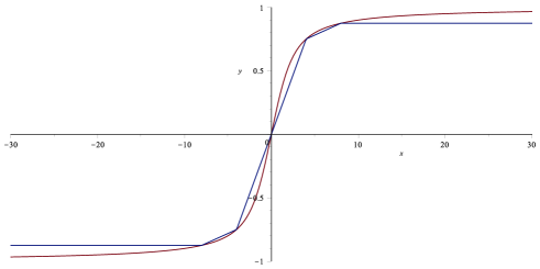
An illustration of the approximation  ¯mNsubscript ¯m𝑁\hbox to0.0pt{\hskip 1.66667pt\leavevmode\hbox{\set@color$\overline{\hbox{}}$}\hss}{\leavevmode\hbox{\set@color$\mathrm{m}$}}_{N} for the secant scheme is shown in Fig. 2. For negative x𝑥x, we expand  ¯mNsubscript ¯m𝑁\hbox to0.0pt{\hskip 1.66667pt\leavevmode\hbox{\set@color$\overline{\hbox{}}$}\hss}{\leavevmode\hbox{\set@color$\mathrm{m}$}}_{N} and  ¯mNsuperscriptsubscript ¯m𝑁\hbox to0.0pt{\hskip 1.66667pt\leavevmode\hbox{\set@color$\overline{\hbox{}}$}\hss}{\leavevmode\hbox{\set@color$\mathrm{m}$}}_{N}^{\prime} such that  ¯mNsubscript ¯m𝑁\hbox to0.0pt{\hskip 1.66667pt\leavevmode\hbox{\set@color$\overline{\hbox{}}$}\hss}{\leavevmode\hbox{\set@color$\mathrm{m}$}}_{N} is odd and  ¯msuperscript ¯m\hbox to0.0pt{\hskip 1.66667pt\leavevmode\hbox{\set@color$\overline{\hbox{}}$}\hss}{\leavevmode\hbox{\set@color$\mathrm{m}$}}^{\prime} is even on \mathbb{R}, i.e.,

 ¯mN(x)= ¯mN(x), ¯mN(x)= ¯mN(x)forx.formulae-sequencesuperscriptsubscript ¯m𝑁𝑥superscriptsubscript ¯m𝑁𝑥formulae-sequencesubscript ¯m𝑁𝑥subscript ¯m𝑁𝑥for𝑥\hbox to0.0pt{\hskip 1.66667pt\leavevmode\hbox{\set@color$\overline{\hbox{}}$}\hss}{\leavevmode\hbox{\set@color$\mathrm{m}$}}_{N}^{\prime}(x)=\hbox to0.0pt{\hskip 1.66667pt\leavevmode\hbox{\set@color$\overline{\hbox{}}$}\hss}{\leavevmode\hbox{\set@color$\mathrm{m}$}}_{N}^{\prime}(-x),\qquad\hbox to0.0pt{\hskip 1.66667pt\leavevmode\hbox{\set@color$\overline{\hbox{}}$}\hss}{\leavevmode\hbox{\set@color$\mathrm{m}$}}_{N}(x)=-\hbox to0.0pt{\hskip 1.66667pt\leavevmode\hbox{\set@color$\overline{\hbox{}}$}\hss}{\leavevmode\hbox{\set@color$\mathrm{m}$}}_{N}(-x)\qquad\text{for}\;x\in\mathbb{R}.
Example 5.1.

For the tangent scheme, we obtain a simple approximation of the derivative  ¯msuperscript ¯m\hbox to0.0pt{\hskip 1.66667pt\leavevmode\hbox{\set@color$\overline{\hbox{}}$}\hss}{\leavevmode\hbox{\set@color$\mathrm{m}$}}^{\prime} already for N=0𝑁0N=0. In this case, using the Langevin model (3) to describe ¯¯\overline{\hbox{}}mm\mathrm{m} and formula (4) for the derivative, we get the approximation

 ¯mN(x)={m0λ3,0x<b,0,xb.superscriptsubscript ¯m𝑁𝑥casessubscript𝑚0𝜆30𝑥𝑏0𝑥𝑏\hbox to0.0pt{\hskip 1.66667pt\leavevmode\hbox{\set@color$\overline{\hbox{}}$}\hss}{\leavevmode\hbox{\set@color$\mathrm{m}$}}_{N}^{\prime}(x)=\begin{cases}\displaystyle\frac{m_{0}\lambda}{3},&0\leq x<b,\\[4.30554pt] 0,&x\geq b.\end{cases} (17)

Then, if

F0(t)={𝒓3:|𝑩(𝒓,t)|<b}subscript𝐹0𝑡𝒓superscript3:𝑩𝒓𝑡𝑏F_{0}(t)=\{\boldsymbol{r}\in\mathbb{R}^{3}\mathrel{\mathop{\mathchar 58\relax}}\;|\boldsymbol{B}(\boldsymbol{r},t)|<b\}

denotes the low field volume (LFV) at time t𝑡t in which the modulus of the magnetic field is smaller than b𝑏b, we obtain in (16) the simple integral equation

uν(t)=μ0m0λ3F0(t)ϱν(𝒓),ddt𝑩(𝒓,t)c(𝒓)𝑑𝒓,subscript𝑢𝜈𝑡subscript𝜇0subscript𝑚0𝜆3subscriptsubscript𝐹0𝑡subscriptbold-italic-ϱ𝜈𝒓dd𝑡𝑩𝒓𝑡𝑐𝒓differential-d𝒓u_{\nu}(t)=-\frac{\mu_{0}m_{0}\lambda}{3}\int_{F_{0}(t)}\left\langle\boldsymbol{\varrho}_{\nu}(\boldsymbol{r}),\frac{\mathrm{d}}{\mathrm{d}t}\boldsymbol{B}(\boldsymbol{r},t)\right\rangle\;c(\boldsymbol{r})\,d\boldsymbol{r},

i.e., the voltage signal uνsubscript𝑢𝜈u_{\nu} is approximately generated by integrating the particle density together with the velocity term ϱν(𝒓),ddt𝑩(𝒓,t)subscriptbold-italic-ϱ𝜈𝒓dd𝑡𝑩𝒓𝑡\left\langle\boldsymbol{\varrho}_{\nu}(\boldsymbol{r}),\frac{\mathrm{d}}{\mathrm{d}t}\boldsymbol{B}(\boldsymbol{r},t)\right\rangle over the LFV F0(t)subscript𝐹0𝑡F_{0}(t).

Refer to caption
Figure 2: Piecewise approximation of the Langevin function L𝐿L by the secant scheme.
Theorem 5.1.

If ¯¯\overline{\hbox{}}mm\mathrm{m} is twice continuously differentiable then, for both, the tangent and the secant approximation scheme, we have the properties:

supx[0,b)| ¯m(x) ¯mN(x)|subscriptsupremum𝑥0𝑏superscript ¯m𝑥superscriptsubscript ¯m𝑁𝑥\displaystyle\sup_{x\in[0,b)}|\hbox to0.0pt{\hskip 1.66667pt\leavevmode\hbox{\set@color$\overline{\hbox{}}$}\hss}{\leavevmode\hbox{\set@color$\mathrm{m}$}}^{\prime}(x)-\hbox to0.0pt{\hskip 1.66667pt\leavevmode\hbox{\set@color$\overline{\hbox{}}$}\hss}{\leavevmode\hbox{\set@color$\mathrm{m}$}}_{N}^{\prime}(x)| supx[0,b)| ¯m′′(x)|maxk{0,,N}(xk+1xk),absentsubscriptsupremum𝑥0𝑏superscript ¯m′′𝑥subscript𝑘0𝑁subscript𝑥𝑘1subscript𝑥𝑘\displaystyle\leq\sup_{x\in[0,b)}|\hbox to0.0pt{\hskip 1.66667pt\leavevmode\hbox{\set@color$\overline{\hbox{}}$}\hss}{\leavevmode\hbox{\set@color$\mathrm{m}$}}^{\prime\prime}(x)|\max_{k\in\{0,\ldots,N\}}(x_{k+1}-x_{k}), (18)
supx[0,b)| ¯m(x) ¯mN(x)|subscriptsupremum𝑥0𝑏 ¯m𝑥subscript ¯m𝑁𝑥\displaystyle\sup_{x\in[0,b)}|\hbox to0.0pt{\hskip 1.66667pt\leavevmode\hbox{\set@color$\overline{\hbox{}}$}\hss}{\leavevmode\hbox{\set@color$\mathrm{m}$}}(x)-\hbox to0.0pt{\hskip 1.66667pt\leavevmode\hbox{\set@color$\overline{\hbox{}}$}\hss}{\leavevmode\hbox{\set@color$\mathrm{m}$}}_{N}(x)| supx[0,b)| ¯m′′(x)|k=0N(xk+1xk)2.absentsubscriptsupremum𝑥0𝑏superscript ¯m′′𝑥superscriptsubscript𝑘0𝑁superscriptsubscript𝑥𝑘1subscript𝑥𝑘2\displaystyle\leq\sup_{x\in[0,b)}|\hbox to0.0pt{\hskip 1.66667pt\leavevmode\hbox{\set@color$\overline{\hbox{}}$}\hss}{\leavevmode\hbox{\set@color$\mathrm{m}$}}^{\prime\prime}(x)|\ \sum_{k=0}^{N}(x_{k+1}-x_{k})^{2}. (19)
Proof.

For both, the tangent and the secant scheme, the mean value theorem on the interval Iksubscript𝐼𝑘I_{k} provides the estimates

| ¯m(x) ¯mN(x)|supxIk| ¯m′′(x)|(xk+1xk).superscript ¯m𝑥superscriptsubscript ¯m𝑁𝑥subscriptsupremum𝑥subscript𝐼𝑘superscript ¯m′′𝑥subscript𝑥𝑘1subscript𝑥𝑘|\hbox to0.0pt{\hskip 1.66667pt\leavevmode\hbox{\set@color$\overline{\hbox{}}$}\hss}{\leavevmode\hbox{\set@color$\mathrm{m}$}}^{\prime}(x)-\hbox to0.0pt{\hskip 1.66667pt\leavevmode\hbox{\set@color$\overline{\hbox{}}$}\hss}{\leavevmode\hbox{\set@color$\mathrm{m}$}}_{N}^{\prime}(x)|\leq\sup_{x\in I_{k}}|\hbox to0.0pt{\hskip 1.66667pt\leavevmode\hbox{\set@color$\overline{\hbox{}}$}\hss}{\leavevmode\hbox{\set@color$\mathrm{m}$}}^{\prime\prime}(x)|(x_{k+1}-x_{k}).

This immediately implies (18). We can use this estimate also to obtain (19):

| ¯m(x) ¯mN(x)| ¯m𝑥subscript ¯m𝑁𝑥\displaystyle|\hbox to0.0pt{\hskip 1.66667pt\leavevmode\hbox{\set@color$\overline{\hbox{}}$}\hss}{\leavevmode\hbox{\set@color$\mathrm{m}$}}(x)-\hbox to0.0pt{\hskip 1.66667pt\leavevmode\hbox{\set@color$\overline{\hbox{}}$}\hss}{\leavevmode\hbox{\set@color$\mathrm{m}$}}_{N}(x)| =|0x( ¯m(x) ¯mN(x))dx|k=0NIk| ¯m(x) ¯mN(x)|dxabsentsuperscriptsubscript0𝑥superscript ¯m𝑥superscriptsubscript ¯m𝑁𝑥differential-d𝑥superscriptsubscript𝑘0𝑁subscriptsubscript𝐼𝑘superscript ¯m𝑥superscriptsubscript ¯m𝑁𝑥differential-d𝑥\displaystyle=\left|\int_{0}^{x}(\hbox to0.0pt{\hskip 1.66667pt\leavevmode\hbox{\set@color$\overline{\hbox{}}$}\hss}{\leavevmode\hbox{\set@color$\mathrm{m}$}}^{\prime}(x)-\hbox to0.0pt{\hskip 1.66667pt\leavevmode\hbox{\set@color$\overline{\hbox{}}$}\hss}{\leavevmode\hbox{\set@color$\mathrm{m}$}}_{N}^{\prime}(x))\,\mathrm{d}x\right|\leq\sum_{k=0}^{N}\int_{I_{k}}|\hbox to0.0pt{\hskip 1.66667pt\leavevmode\hbox{\set@color$\overline{\hbox{}}$}\hss}{\leavevmode\hbox{\set@color$\mathrm{m}$}}^{\prime}(x)-\hbox to0.0pt{\hskip 1.66667pt\leavevmode\hbox{\set@color$\overline{\hbox{}}$}\hss}{\leavevmode\hbox{\set@color$\mathrm{m}$}}_{N}^{\prime}(x)|\,\mathrm{d}x
supx[0,b)| ¯m′′(x)|k=0N(xk+1xk)2.absentsubscriptsupremum𝑥0𝑏superscript ¯m′′𝑥superscriptsubscript𝑘0𝑁superscriptsubscript𝑥𝑘1subscript𝑥𝑘2\displaystyle\leq\sup_{x\in[0,b)}|\hbox to0.0pt{\hskip 1.66667pt\leavevmode\hbox{\set@color$\overline{\hbox{}}$}\hss}{\leavevmode\hbox{\set@color$\mathrm{m}$}}^{\prime\prime}(x)|\ \sum_{k=0}^{N}(x_{k+1}-x_{k})^{2}. (20)

5.2 Selection of the nodes

The nodes x1,,xNsubscript𝑥1subscript𝑥𝑁x_{1},\ldots,x_{N} in the interval (0,b)0𝑏(0,b) can be chosen in several different ways. Based on our result in Theorem 5.1, we provide two simple options:

  • 1)

    Equidistant points (the simplest choice):

    xk=bkN+1,k{0,,N+1}.formulae-sequencesubscript𝑥𝑘𝑏𝑘𝑁1𝑘0𝑁1x_{k}=\frac{b\,k}{N+1},\qquad k\in\{0,\ldots,N+1\}.
  • 2)

    L1subscript𝐿1L_{1}-optimal points: choose x1,,xNsubscript𝑥1subscript𝑥𝑁x_{1},\ldots,x_{N} in (0,b)0𝑏(0,b) such that the L1superscript𝐿1L^{1}-norm

    0b| ¯m(x) ¯mN(x)|dxsuperscriptsubscript0𝑏superscript ¯m𝑥superscriptsubscript ¯m𝑁𝑥differential-d𝑥\int_{0}^{b}|\hbox to0.0pt{\hskip 1.66667pt\leavevmode\hbox{\set@color$\overline{\hbox{}}$}\hss}{\leavevmode\hbox{\set@color$\mathrm{m}$}}^{\prime}(x)-\hbox to0.0pt{\hskip 1.66667pt\leavevmode\hbox{\set@color$\overline{\hbox{}}$}\hss}{\leavevmode\hbox{\set@color$\mathrm{m}$}}_{N}^{\prime}(x)|\,\mathrm{d}x

    is minimized.

Theorem 5.1 ensures that both choices lead to a uniform convergence of  ¯mNsuperscriptsubscript ¯m𝑁\hbox to0.0pt{\hskip 1.66667pt\leavevmode\hbox{\set@color$\overline{\hbox{}}$}\hss}{\leavevmode\hbox{\set@color$\mathrm{m}$}}_{N}^{\prime} towards  ¯msuperscript ¯m\hbox to0.0pt{\hskip 1.66667pt\leavevmode\hbox{\set@color$\overline{\hbox{}}$}\hss}{\leavevmode\hbox{\set@color$\mathrm{m}$}}^{\prime} on the interval [0,b)0𝑏[0,b). The L1subscript𝐿1L_{1}-optimized variant yields a better approximation quality for the derivative  ¯msuperscript ¯m\hbox to0.0pt{\hskip 1.66667pt\leavevmode\hbox{\set@color$\overline{\hbox{}}$}\hss}{\leavevmode\hbox{\set@color$\mathrm{m}$}}^{\prime} as well as for the magnetization function ¯¯\overline{\hbox{}}mm\mathrm{m}. This can be seen particularly in the estimate (20), in which an L1subscript𝐿1L_{1}- optimal ensemble makes the second inequality redundant.

In case of the tangent scheme, we give an explicit formula for the L1subscript𝐿1L_{1}-norm. We assume that the derivative  ¯msuperscript ¯m\hbox to0.0pt{\hskip 1.66667pt\leavevmode\hbox{\set@color$\overline{\hbox{}}$}\hss}{\leavevmode\hbox{\set@color$\mathrm{m}$}}^{\prime} is positive and strictly monotonically decreasing when x0𝑥0x\geq 0. This is indeed the case if the magnetization ¯¯\overline{\hbox{}}mm\mathrm{m} is given as in (3) by the Langevin model. Then, we get the explicit formula

0b| ¯m(x) ¯mN(x)|dxsuperscriptsubscript0𝑏superscript ¯m𝑥superscriptsubscript ¯m𝑁𝑥differential-d𝑥\displaystyle\int_{0}^{b}|\hbox to0.0pt{\hskip 1.66667pt\leavevmode\hbox{\set@color$\overline{\hbox{}}$}\hss}{\leavevmode\hbox{\set@color$\mathrm{m}$}}^{\prime}(x)-\hbox to0.0pt{\hskip 1.66667pt\leavevmode\hbox{\set@color$\overline{\hbox{}}$}\hss}{\leavevmode\hbox{\set@color$\mathrm{m}$}}_{N}^{\prime}(x)|\,\mathrm{d}x =k=0NIk| ¯m(x)sk|dxabsentsuperscriptsubscript𝑘0𝑁subscriptsubscript𝐼𝑘superscript ¯m𝑥subscript𝑠𝑘differential-d𝑥\displaystyle=\sum_{k=0}^{N}\int_{I_{k}}|\hbox to0.0pt{\hskip 1.66667pt\leavevmode\hbox{\set@color$\overline{\hbox{}}$}\hss}{\leavevmode\hbox{\set@color$\mathrm{m}$}}^{\prime}(x)-s_{k}|\,\mathrm{d}x
=k=0N(xkxk+xk+12 ¯m(x)dxxk+xk+12xk+1 ¯m(x)dx)absentsuperscriptsubscript𝑘0𝑁superscriptsubscriptsubscript𝑥𝑘subscript𝑥𝑘subscript𝑥𝑘12superscript ¯m𝑥differential-d𝑥superscriptsubscriptsubscript𝑥𝑘subscript𝑥𝑘12subscript𝑥𝑘1superscript ¯m𝑥differential-d𝑥\displaystyle=\sum_{k=0}^{N}\left(\int_{x_{k}}^{\frac{x_{k}+x_{k+1}}{2}}\hbox to0.0pt{\hskip 1.66667pt\leavevmode\hbox{\set@color$\overline{\hbox{}}$}\hss}{\leavevmode\hbox{\set@color$\mathrm{m}$}}^{\prime}(x)\,\mathrm{d}x-\int_{\frac{x_{k}+x_{k+1}}{2}}^{x_{k+1}}\hbox to0.0pt{\hskip 1.66667pt\leavevmode\hbox{\set@color$\overline{\hbox{}}$}\hss}{\leavevmode\hbox{\set@color$\mathrm{m}$}}^{\prime}(x)\,\mathrm{d}x\right)
=k=0N(2 ¯m(xk+xk+12) ¯m(xk+1) ¯m(xk))=F(x1,,xN).absentsuperscriptsubscript𝑘0𝑁2 ¯msubscript𝑥𝑘subscript𝑥𝑘12 ¯msubscript𝑥𝑘1 ¯msubscript𝑥𝑘𝐹subscript𝑥1subscript𝑥𝑁\displaystyle=\sum_{k=0}^{N}\left(2\,\hbox to0.0pt{\hskip 1.66667pt\leavevmode\hbox{\set@color$\overline{\hbox{}}$}\hss}{\leavevmode\hbox{\set@color$\mathrm{m}$}}(\textstyle\frac{x_{k}+x_{k+1}}{2})-\hbox to0.0pt{\hskip 1.66667pt\leavevmode\hbox{\set@color$\overline{\hbox{}}$}\hss}{\leavevmode\hbox{\set@color$\mathrm{m}$}}(x_{k+1})-\hbox to0.0pt{\hskip 1.66667pt\leavevmode\hbox{\set@color$\overline{\hbox{}}$}\hss}{\leavevmode\hbox{\set@color$\mathrm{m}$}}(x_{k})\right)=F(x_{1},\ldots,x_{N}).

Thus, in order to find the ensamble in which the L1superscript𝐿1L^{1}-norm gets minimal, we only have to minimize the functional F𝐹F.

5.3 Full discretization and model-based imaging matrix

We assume to have T𝑇T discrete time measurements 𝒖ν=(uν(t1),,uν(tT))subscript𝒖𝜈subscript𝑢𝜈subscript𝑡1subscript𝑢𝜈subscript𝑡𝑇\boldsymbol{u}_{\nu}=(u_{\nu}(t_{1}),\dots,u_{\nu}(t_{T})) of the voltage signal uνsubscript𝑢𝜈u_{\nu}. To discretize the particle density c(𝒓)𝑐𝒓c(\boldsymbol{r}), we use the representation

c(𝒓)=k=1Kckδk(𝒓)𝑐𝒓superscriptsubscript𝑘1𝐾subscript𝑐𝑘subscript𝛿𝑘𝒓c(\boldsymbol{r})=\sum_{k=1}^{K}c_{k}\delta_{k}(\boldsymbol{r})

of c𝑐c in a given set of basis functions δksubscript𝛿𝑘\delta_{k}, k=1,,K𝑘1𝐾k=1,\ldots,K. In our implementation, we use a pixel basis, i.e., δk=χQksubscript𝛿𝑘subscript𝜒subscript𝑄𝑘\delta_{k}=\chi_{Q_{k}} for rectangular pixel regions Qksubscript𝑄𝑘Q_{k} centered at the pixel locations 𝒓ksubscript𝒓𝑘\boldsymbol{r}_{k}. Therefore, we have ck=c(𝒓k)subscript𝑐𝑘𝑐subscript𝒓𝑘c_{k}=c(\boldsymbol{r}_{k}).

The approximate model equation stated in (14) can now be discretized as

uν(tj)=n=0Nsnk=1KckFn(tj)Kν(𝒓,tj)δk(𝒓)𝑑𝒓.subscript𝑢𝜈subscript𝑡𝑗superscriptsubscript𝑛0𝑁subscript𝑠𝑛superscriptsubscript𝑘1𝐾subscript𝑐𝑘subscriptsubscript𝐹𝑛subscript𝑡𝑗subscript𝐾𝜈𝒓subscript𝑡𝑗subscript𝛿𝑘𝒓differential-d𝒓u_{\nu}(t_{j})=\sum_{n=0}^{N}s_{n}\sum_{k=1}^{K}c_{k}\int_{F_{n}(t_{j})}K_{\nu}(\boldsymbol{r},t_{j})\delta_{k}(\boldsymbol{r})d\boldsymbol{r}.

We denote by Sν,nT×Ksubscript𝑆𝜈𝑛superscript𝑇𝐾S_{\nu,n}\in\mathbb{R}^{T\times K} the rectangular matrix with the entries

(Sν,n)j,k=Fn(tj)Kν(𝒓,tj)δk(𝒓)𝑑𝒓=Fn(tj)QkKν(𝒓,tj)𝑑𝒓.subscriptsubscript𝑆𝜈𝑛𝑗𝑘subscriptsubscript𝐹𝑛subscript𝑡𝑗subscript𝐾𝜈𝒓subscript𝑡𝑗subscript𝛿𝑘𝒓differential-d𝒓subscriptsubscript𝐹𝑛subscript𝑡𝑗subscript𝑄𝑘subscript𝐾𝜈𝒓subscript𝑡𝑗differential-d𝒓(S_{\nu,n})_{j,k}=\int_{F_{n}(t_{j})}K_{\nu}(\boldsymbol{r},t_{j})\delta_{k}(\boldsymbol{r})d\boldsymbol{r}=\int_{F_{n}(t_{j})\cap Q_{k}}K_{\nu}(\boldsymbol{r},t_{j})d\boldsymbol{r}.

Then, a model-based discrete imaging equation to recover the particle concentration can be written as

𝒖ν=(n=0NsnSν,n)𝒄=Sν𝒄,subscript𝒖𝜈superscriptsubscript𝑛0𝑁subscript𝑠𝑛subscript𝑆𝜈𝑛𝒄subscript𝑆𝜈𝒄\boldsymbol{u}_{\nu}=\left(\sum_{n=0}^{N}s_{n}S_{\nu,n}\right)\boldsymbol{c}=S_{\nu}\boldsymbol{c}, (21)

where 𝒄=(c1,,cK)𝒄subscript𝑐1subscript𝑐𝐾\boldsymbol{c}=(c_{1},\dots,c_{K}) are the sought concentration values and SνT×Ksubscript𝑆𝜈superscript𝑇𝐾S_{\nu}\in\mathbb{R}^{T\times K} is the modeled system matrix for the receive coil ν𝜈\nu.

5.4 Algebraic reconstruction of the particle concentration

In order to solve the system of equations (21) for the particle concentration 𝒄𝒄\boldsymbol{c}, we combine the information of all V𝑉V receive coils. In this way, we get the system

(𝒖1𝒖V)𝒖=(S1SV)S𝒄.subscriptmatrixsubscript𝒖1subscript𝒖𝑉𝒖subscriptmatrixsubscript𝑆1subscript𝑆𝑉𝑆𝒄\underbrace{\begin{pmatrix}\boldsymbol{u}_{1}\\ \vdots\\ \boldsymbol{u}_{V}\end{pmatrix}}_{\boldsymbol{u}}=\underbrace{\begin{pmatrix}S_{1}\\ \vdots\\ S_{V}\end{pmatrix}}_{S}\boldsymbol{c}.

From this system we extract the particle concentration 𝒄𝒄\boldsymbol{c} by calculating the solution of the normal equation STS𝒄=ST𝒖superscript𝑆𝑇𝑆𝒄superscript𝑆𝑇𝒖S^{T}S\boldsymbol{c}=S^{T}\boldsymbol{u} iteratively using the LSQR algorithm together with an early stopping rule.

Remark 4.

Although the particle reconstruction in MPI is in general an ill-posed inverse problem [4, 13, 21], at that stage, we did not incorporate additional regularization for the solution of the linear system 𝒖=S𝒄𝒖𝑆𝒄\boldsymbol{u}=S\boldsymbol{c}. The various discretization steps applied in our model and the early stopping of the LSQR procedure already provide a certain regularization of the problem. In combination with our model, one could of course apply also more advanced regularization schemes as for instance described in [26].

6 Experiments

Based on the phantom presented in Fig. 3a, two types of magnetic field topologies are used to study the influence on the reconstruction: an ideal rotating FFL magnetic field, represented by a few low-degree spherical harmonics, as described in Section 3.3; and a realistic one, obtained from either a realistic numerical model of the magnetic coil or from measurements. A concrete example of such a realistic field is given in Section 3.5.
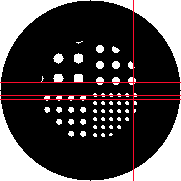
Refer to caption
(a)
Refer to caption
(b)
Refer to caption
(c)
Figure 3: Ideal and realistic rotating FFL’s: LABEL:sub@subfig:phantom A phantom composed of circles (in white) of 4, 6, 8 and 10 mm diameter inside a 100 mm diameter circle. The reconstructions along the illustrated horizontal and vertical lines are shown in Fig. 7, 9 and 11. LABEL:sub@subfig:LFV_Ideal and LABEL:sub@subfig:LFV_Real show the LFV (in red) with a field amplitude smaller than 2 mT for an ideal and a realistic field topology, respectively (frotsubscript𝑓rotf_{\mathrm{rot}}=100 Hz).

The influence of the higher degree spherical harmonics on the LFV can be observed by comparing Fig. 3b which illustrates the LFV at 2 mT for ideal topologies at a given time t=17.25μ𝑡17.25𝜇t=17.25~{}\mus in our sequence, with Fig. 3c which shows the corresponding LFV for the realistic field topology used afterwards in our simulations. The LFV compared to an ideal FFL is slightly bended and interrupted on the upper part. To highlight the effect of these differences on the reconstructed particle concentrations, we run now experiments comparing side by side the images obtained either by a filtered back-projection (FBP) for ideal and realistic fields or by our algebraic method.

6.1 General experimental parameters

For all the presented results, the drive field frequency is fixed at fdsubscript𝑓df_{\mathrm{d}}=25 kHz and the line rotation frequency frotsubscript𝑓rotf_{\mathrm{rot}} is varied from 100 Hz to 1000 Hz. Due to a RAM limitation of 1 TB in our system, a rotation frequency of 10 Hz has not be conducted. Thus, 250 and 25 projections were used for the 100 Hz and 1000 Hz reconstruction, respectively. It is common to set the drive frequency between <1 kHz to 150 kHz and the rotation frequency from <1 Hz to 100 Hz. The sampling frequency is set to 8 Mhz (4 Mhz for FBP), thus obtaining 160 points per projection (80 for FBP) and emulating the common properties of the acquisition hardware used. Note that in order to do a frequency filtering on the measured signal, the whole rotation was always simulated to obtain a perfectly resolved spectra. Indeed, the hardware of an actual MPI scanner always filters out a frequency range around fdsubscript𝑓df_{\mathrm{d}}. To reproduce this effect, we always removed all the information below 1.4 fdsubscript𝑓df_{\mathrm{d}} from the measured signal. Furthermore, a Gaussian noise was added to all simulations. For the signal simulation, a spatial discretization of 1×1×11111\times 1\times 1 mm3 was used, whereas a discretization of 1.3×1.3×11.31.311.3\times 1.3\times 1 mm3 was used for the system matrix. The solution of the proposed discretized MPI model (21) was solved using Matlab’s LSQR implementation, which was always stopped after 202020 iterations. This has been optimized on a simulation using a rotation frequency frotsubscript𝑓rotf_{\mathrm{rot}} of 100100100 Hz, a threshold of b=10𝑏10b=10 mT and kept constant for all further tests.

6.2 Comparison with the filtered back projection

Refer to caption
(a)
Refer to caption
(b)
Figure 4: Two sinograms of the phantom from Fig. 3a used as input data for the algorithms. LABEL:sub@subfig:sino_normal Sinogram of a phantom in which the maximal displacement of the Radon transform is adapted to the support of the phantom. It is used to generate the reconstruction shown in Table 4. LABEL:sub@subfig:sino_padded Same sinogram padded with zero, to increase the reconstruction area of the FBP.

We compare our method with the filtered back projection (FBP), which is commonly used for FFL systems to perform the image reconstruction [1, 20]. The FBP implementation of Matlab (Version 7.11.0) was used to performed the first test. The Radon projections are obtained by the reconstruction steps described in Remark 2, using half a period of a drive field sweep with frequency fdsubscript𝑓df_{\mathrm{d}} for fixed approximate angles α2πfrott𝛼2𝜋subscript𝑓rot𝑡\alpha\approx 2\pi f_{\mathrm{rot}}t and for discrete s=d2gsin(2πfdt)𝑠𝑑2𝑔2𝜋subscript𝑓d𝑡s=\frac{d}{2g}\sin\big{(}2\pi f_{\mathrm{d}}t) in a subinterval of [d2g,d2g]𝑑2𝑔𝑑2𝑔[-\frac{d}{2g},\frac{d}{2g}]. The so obtained Radon data is assembled into a sinogram and then reconstructed using the FBP.

The sinogram obtained using the ideal model of a rabbit sized FFL MPI scanner [2] is presented in Fig. 4a. To fully asses the differences between the reconstruction methods over the whole scanner opening, the sinogram is further padded with zeros, as shown in Fig. 4b.

The results of the FBP are compared with the images obtained by our method. The system matrix Sνsubscript𝑆𝜈S_{\nu} for the algebraic reconstruction in (21) is constructed using the threshold b=10mT𝑏10mTb=10~{}\mathrm{mT} and the secant approximation scheme with N=30𝑁30N=30 equidistant nodes for the discretization of the Langevin function. The information about the magnetic field 𝑩(𝒓,t)𝑩𝒓𝑡\boldsymbol{B}(\boldsymbol{r},t) and its time-derivative is obtained by measurements or simulations.

Tables 4 and 5 highlight the main advantages of our method. Indeed, the presented model-based reconstruction method compensates the main artefacts introduced by the idealized assumptions in the FBP reconstruction. Looking at the Table 4, the rotation artifacts which appeared in all images produced by the FBP independently of the field complexity and only linked to the continuous rotation of the LFV during an acquisition are compensated. The distortion artifacts visible on both Tables, introduced by the complex field topology are also corrected. This can be further observed by the corrected distances between two points of the phantom.

Ideal FFL and FBP Realistic FFL and FBP Realistic FFL & our method

100 Hz

[Uncaptioned image] [Uncaptioned image] [Uncaptioned image]

1000 Hz

[Uncaptioned image] [Uncaptioned image] [Uncaptioned image]
Table 4: Comparison of reconstructions for different rotating FFL topologies using frot=100subscript𝑓rot100f_{\mathrm{rot}}=100 Hz (1. row), frot=1000subscript𝑓rot1000f_{\mathrm{rot}}=1000 Hz (2. row), and identically chosen fields of view.
Ideal FFL and FBP Realistic FFL and FBP Realistic FFL & our method

100 Hz

[Uncaptioned image] [Uncaptioned image] [Uncaptioned image]
Table 5: Reconstructions of Table 4 (first row) using an enlarged field of view. A sinogram padded with zero, as illustrated in Fig. 4b, is used to extend the reconstruction area of the FBP.

6.3 Influence of amplitude threshold

We further study the influence of the threshold b𝑏b on the reconstruction quality. In Fig. 5 we can see how this threshold determines the volume of the LFV used in the discrete imaging equation (21) to model the generation of the MPI signal.
Refer to caption11-10.50.5-0.5000.50.50.5111
(a)
Refer to caption11-10.50.5-0.5000.50.50.5111
(b)
Figure 5: Influence of the threshold b𝑏b on the information included in the system matrix Sνsubscript𝑆𝜈S_{\nu} for frotsubscript𝑓rotf_{\mathrm{rot}}=100 Hz at t=17.25 μ𝜇\mus using the secant approximation scheme with N=30𝑁30N=30 equidistant nodes. The normalized entries of the system function Sνsubscript𝑆𝜈S_{\nu} are displayed: LABEL:sub@subfig:SM_2mT for a threshold of b=2𝑏2b=2 mT and LABEL:sub@subfig:SM_10mT for a threshold of b=10𝑏10b=10 mT.
Refer to caption
(a)
Refer to caption
(b)
Refer to caption
(c)
Refer to caption
(d)
Refer to caption
(e)
Refer to caption
(f)
Figure 6: Reconstruction with thresholds 1, 2, 3, 4, 5 and 10 mT shown in LABEL:sub@subfig:Thresholds_1mT to LABEL:sub@subfig:Thresholds_10mT.
0123105absentsuperscript105\cdot 10^{-5}2nd line0123105absentsuperscript105\cdot 10^{-5}1st Line1 mT2 mT3 mT4 mT10 mTPhantom0123105absentsuperscript105\cdot 10^{-5}3rd Line002020204040406060608080801001001001201201201401401400123105absentsuperscript105\cdot 10^{-5}4th Line
Figure 7: Comparison of the line profiles (as shown in Fig. 3a) for the reconstructions obtained with our method using different thresholds b𝑏b and the original phantom.

The reconstructions in Fig. 6 and the line profiles in Fig. 7 show that the choice of the threshold b𝑏b has a strong impact on the reconstruction quality in the entire field of view (FOV) when b𝑏b is in the range 1 to 4 mT. On the other hand, if b𝑏b is between 4 and 10 mT only small differences are visible on the periphery of the FOV. Thus, in this example a threshold b𝑏b of 10 mT is sufficient, and a threshold of 4 mT yields already very good results for the central part of the FOV. Note that a smaller threshold is desirable from a computational point of view in order to benefit from a sparser representation of the system matrix Sνsubscript𝑆𝜈S_{\nu}.

6.4 Discretization effects

In two additional tests, we study discretization effects on the reconstruction. In the first test, we search for the optimal number of equidistant nodes N𝑁N for the piecewise approximation of the Langevin function in the tangential approximation scheme on an example with frotsubscript𝑓rotf_{\mathrm{rot}}=100 Hz and a threshold b=10𝑏10b=10 mT. The corresponding results are illustrated in Fig. 8 and Fig. 9. It is visible that already for N=8𝑁8N=8 the piecewise approximation of the Langevin function provides acceptable reconstructions.

In a second experiment, we test three different discretization techniques for the Langevin function on an example with frotsubscript𝑓rotf_{\mathrm{rot}}=100 Hz, threshold b=10𝑏10b=10 mT and N=30𝑁30N=30 nodes. As shown in Figure 10 and Fig. 11, all three discretizations provide comparable reconstruction results.
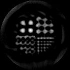
Refer to caption
(a)
Refer to caption
(b)
Refer to caption
(c)
Refer to caption
(d)
Figure 8: Reconstruction with different number N𝑁N of nodes in the discretization of the Langevin function. The results given here are for 3, 4, 8 and 30 nodes.
0123105absentsuperscript105\cdot 10^{-5}2nd line0123105absentsuperscript105\cdot 10^{-5}1st Line34830Phantom0123105absentsuperscript105\cdot 10^{-5}3rd Line002020204040406060608080801001001001201201201401401400123105absentsuperscript105\cdot 10^{-5}4th Line
Figure 9: Line profiles (as shown in Fig. 3a) for the reconstructions obtained with our method using different numbers N𝑁N for the approximation of the Langevin function.
Refer to caption
(a)
Refer to caption
(b)
Refer to caption
(c)
Figure 10: Reconstruction with three different discretization schemes. LABEL:sub@subfig:thr1 Secant, equidistant; LABEL:sub@subfig:thr2 Tangent, equidistant; LABEL:sub@subfig:thr3 Tangent, L1subscript𝐿1L_{1}-optimal.
0123105absentsuperscript105\cdot 10^{-5}2nd line0123105absentsuperscript105\cdot 10^{-5}1st Line Secant equidistant Tangent equidistant Tangent L1superscript𝐿1L^{1}-optimal Phantom0123105absentsuperscript105\cdot 10^{-5}3rd Line002020204040406060608080801001001001201201201401401400123105absentsuperscript105\cdot 10^{-5}4th Line
Figure 11: Line profiles (as shown in Fig. 3a) for the reconstructions obtained with our method using the three discretization techniques given in Fig. 10.

7 Conclusion

We introduced a new 3D modelling framework for magnetic particle imaging that includes classical MPI models based on ideal 1D-FFP and FFL magnetic fields, as well as realistic magnetic field topologies. Via expansions in spherical harmonics, this framework allows to incorporate realistic magnetic fields in the imaging model such that the reconstruction process can be adapted to a given scanner topology. In this sense, our framework can be regarded as a hybrid model-based approach for MPI in which the applied magnetic fields are measured in a preliminary calibration step and then included in the 3D model.

Compared to an ideal FFP or FFL topology, the magnetic fields generated in real MPI scanners have distortions that lead to distorted low-field volumes. Our model-based approach is able to deal with these distortions and can generally be applied for magnetic fields that are parallel to their velocity field. We showed how this new 3D model can be approximated and discretized numerically in order to obtain a finite system matrix for the reconstruction of the magnetic particles.

To obtain the final magnetic particle distribution, we inverted the resulting system matrix algebraically using a finite number of LSQR iterations and no further tuning. This was sufficient to evaluate the enhanced reconstruction properties of our proposed model, leaves however room for further improvements. In particular, the incorporation of more advanced regularization techniques is likely to have an additional positive effect on the reconstruction quality of our model.

Acknowledgements

The authors of this article were involved in the activities of the DFG-funded scientific network MathMPI (ER777/1-1) and thank the German Research Foundation for the support.

References

References

  • [1] K. Bente, M. Weber, M. Graeeser, T. F. Sattel, M. Erbe, and T. M. Buzug. Electronic field free line rotation and relaxation deconvolution in magnetic particle imaging. IEEE Trans. Med. Imag., 34(2):644–651, 2014.
  • [2] G. Bringout. Field Free Line Magnetic Particle Imaging: Characterisation and imaging device up-scaling. PhD thesis, Universität zu Lübeck, 2016.
  • [3] G. Bringout and T. M. Buzug. A robust and compact representation for magnetic fields in magnetic particle imaging. Biomedical Engineering, 59:646–650, 2014.
  • [4] W. Erb, A. Weinmann, M. Ahlborg, C. Brandt, G. Bringout, T. M. Buzug, J. Frikel, C. Kaethner, T. Knopp, T. März, M. Möddel, M. Storath, and A. Weber. Mathematical Analysis of the 1D Model and Reconstruction Schemes for Magnetic Particle Imaging. Inverse Problems, 34:055012, 2018.
  • [5] M. Erbe. Field Free Line Magnetic Particle Imaging. Springer Vieweg, 2014.
  • [6] B. Gleich and J. Weizenecker. Tomographic imaging using the nonlinear response of magnetic particles. Nature, 435:1214–1217, 2005.
  • [7] P. Goodwill and S. Conolly. The X-space formulation of the magnetic particle imaging process: 1-D signal, resolution, bandwidth, SNR, SAR, and magnetostimulation. IEEE Trans. Med. Imaging, 29:1851–1859, 2010.
  • [8] P. Goodwill and S. Conolly. Multidimensional X-space magnetic particle imaging. IEEE Trans. Med. Imaging, 30:1581–1590, 2011.
  • [9] M. Grüttner, T. Knopp, J. Franke, M. Heidenreich, J. Rahmer, A. Halkola, C. Kaethner, J. Borgert, and T. M. Buzug. On the formulation of the image reconstruction problem in magnetic particle imaging. Biomedical Engineering, 58(6):583–591, 2013.
  • [10] J. D. Jackson. Classical electrodynamics. Wiley, New York, NY, 3rd ed. edition, 1999.
  • [11] C. Kaethner, W. Erb, M. Ahlborg, P. Szwargulski, T. Knopp, and T. M. Buzug. Non-equispaced system matrix acquisition for magnetic particle imaging based on Lissajous node points. IEEE Trans. Med. Imag., 35(11):2476–2485, 2016.
  • [12] T. Kluth. Mathematical models for magnetic particle imaging. Inverse Problems, 34(8):083001, 2018.
  • [13] T. Kluth, B. Jin, and G. Li. On the degree of ill-posedness of multi-dimensional magnetic particle imaging. Inverse Problems, 34(9):095006, 2018.
  • [14] T. Kluth, P. Szwargulski, and T. Knopp. Towards accurate modeling of the multidimensional magnetic particle imaging physics. New Journal of Physics, 21(10):103032, 2019.
  • [15] T. Knopp, S. Biederer, T. Sattel, J. Weizenecker, B. Gleich, J. Borgert, and T. M. Buzug. Trajectory analysis for magnetic particle imaging. Phys. Med. Biol., 54:385–397, 2009.
  • [16] T. Knopp and T. M. Buzug. Magnetic Particle Imaging: An Introduction to Imaging Principles and Scanner Instrumentation. Springer, 2012.
  • [17] T. Knopp, M. Erbe, S. Biederer, T. F. Sattel, and T. M. Buzug. Efficient generation of a magnetic field-free line. Medical Physics, 37:35–38, 2010.
  • [18] T. Knopp, M. Erbe, T. Sattel, S. Biederer, and T. M. Buzug. A Fourier slice theorem for magnetic particle imaging using a field-free line. Inverse Problems, 27:095004, 2011.
  • [19] T. Knopp, N. Gdaniec, and M. Möddel. Magnetic particle imaging: from proof of principle to preclinical applications. Phys. Med. Biol., 64(14):124–178, 2017.
  • [20] J. J. Konkle, P. W. Goodwill, E. U. Saritas, B. Zheng, K. Lu, and S. M. Conolly. Twenty-fold acceleration of 3d projection reconstruction MPI. Biomedical Engineering, 58(6):565–576, 2013.
  • [21] T. März and A. Weinmann. Model-based reconstruction for magnetic particle imaging in 2d and 3d. Inverse Problems and Imaging, 10(4), 2016.
  • [22] N. Panagiotopoulos, R. Duschka, M. Ahlborg, G. Bringout, C. Debbeler, M. Graeser, C. Kaethner, K. Lüdtke-Buzug, H. Medimagh, J. Stelzner, T. M. Buzug, J. Barkhausen, F. M. Vogt, and J. Haegele. Magnetic particle imaging - current developments and future directions. International Journal of Nanomedicine, 10:3097–3114, 2015.
  • [23] J. Rahmer, J. Weizenecker, B. Gleich, and J. Borgert. Signal encoding in magnetic particle imaging: properties of the system function. BMC Medical Imaging, 9:4, 2009.
  • [24] E. Saritas, P. Goodwill, L. Croft, J. Konkle, K. Lu, B. Zheng, and S. Conolly. Magnetic particle imaging (MPI) for NMR and MRI researchers. J. of Magnetic Resonance, 229:116–126, 2013.
  • [25] H. Schomberg. Magnetic particle imaging: model and reconstruction. In 2010 IEEE Inter- national Symposium on Biomedical Imaging: From Nano to Macro, pages 992–995, 2010.
  • [26] M. Storath, C. Brandt, M. Hofmann, T. Knopp, J. Salamon, A. Weber, and A. Weinmann. Edge preserving and noise reducing reconstruction for magnetic particle imaging. IEEE Trans. Med. Imag., 36(1):74–85, 2017.
  • [27] J. Weizenecker. The Fokker–Planck equation for coupled Brown–Néel-rotation. Phys. Med. Biol., 63(3):035004, 2018.
  • [28] J. Weizenecker, B. Gleich, and J. Borgert. Magnetic particle imaging using a field free line. Journal of Physics D: Applied Physics, 41(10):105009, 2008.
  • [29] J. Weizenecker, B. Gleich, J. Rahmer, H. Dahnke, and J. Borgert. Three-dimensional real-time in vivo magnetic particle imaging. Phys. Med. Biol., 54(5):L1–L10, 2009.
AS
amplitude spectrum
ASD
amplitude spectral density
ART
algebraic reconstruction technique
BEM
boundary element method
CS
coordinate system
CT
computed tomography
DCT
discrete cosine transform
DFT
discrete Fourier transform
FBP
filtered back-projection
FC
Fourier coefficient
FEM
finite element method
FFL
field-free line
FFP
field-free point
FOV
field of view
HMIEFA
highest maximal induced electrical field amplitude
ISIC
idealised scanner made of idealised coils
LFV
low-field volume
LNA
low-noise amplifier
MC
multipole coefficient
MIEFA
maximal induced electrical field amplitude
MPI
magnetic particle imaging
MRI
magnetic resonance imaging
MSE
multipole series expansion
nHMIEFA
normalised highest maximal induced electrical field amplitude
nMIEFA
normalised maximal induced electrical field amplitude
PNS
peripheral nerve stimulation
PS
power spectrum
PSD
power spectral density
QPQC
quadratic programming problem with quadratic constrains
RMS
root mean square
SAR
specific absorption rate
SF
system function
SHC
spherical harmonic coefficient
SPION
superparamagnetic iron oxide nanoparticle
SPIONs
superparamagnetic iron oxide nanoparticles
SNR
signal to noise ratio
SHSE
spherical harmonic series expansion
THD
total harmonic distortion
tSF
truncated system function