Abstract

In the previous papers, it is pointed out that a supersymmetric double-well matrix model corresponds to a two-dimensional type IIA superstring theory on a Ramond-Ramond background at the level of correlation functions. This was confirmed by agreement between their planar correlation functions. The supersymmetry in the matrix model corresponds to the target space supersymmetry and it is shown to be spontaneously broken by nonperturbative effect. Furthermore, in the matrix model we computed one-point functions of single-trace operators to all order of genus expansion in its double scaling limit. We found that this expansion is stringy and not Borel summable and hence there arises an ambiguity in applying the Borel resummation technique. We confirmed that resurgence works here, namely this ambiguity in perturbative series in a zero-instanton sector is exactly canceled by another ambiguity in a one-instanton sector obtained by instanton calculation. In this paper we extend this analysis and study resurgence structure of the two-point functions of the single trace operators. By using results in the random matrix theory, we derive two-point functions at arbitrary genus and see that the perturbative series in the zero-instanton sector again has an ambiguity. We find that the two-point functions inevitably have logarithmic singularity even at higher genus. In this derivation we obtain a new result of the two-point function expressed by the one-point function at the leading order in the soft-edge scaling limit of the random matrix theory. We also compute an ambiguity in the one-instanton sector by using the Airy kernel, and confirm that ambiguities in both sectors cancel each other at the leading order in the double scaling limit. We thus clarify resurgence structure of the two-point functions in the supersymmetric double-well matrix model.

1 Introduction

So far string theory has been defined only perturbatively except peculiar cases with much higher symmetry or much fewer degrees of freedom. It is, however, understood that its nonperturbative effect is more relevant than in field theory and that they would play an important role in determining vacuum structure of string theory.

On the other hand, resurgence [1, 2, 3, 4, 5, 6, 7, 8] has attracted lots of attention because it enables us to extract nonperturbative information of our interest from data of higher-order perturbative expansion. Thus it is reasonable to expect that resurgence provides a powerful tool in analyzing nonperturbative aspects of string theory with respect to the string coupling constant. However, when we try to apply the resurgence to string theory, one of the biggest problems is difficulty in getting higher-genus contribution. In general, in order to obtain information on nonperturbative effect precisely, we need details of higher order in perturbative expansion, which are in general hard to deduce. In order to find perturbative expansion up to higher genus, we may consider theory with higher symmetry or without much degrees of freedom. Then we in turn have another problem that in such cases perturbative expansion itself often behaves well and that resurgence may not work to extract nonperturbative information from it.

Another interest in resurgence is connection to nontrivial phenomena in which nonperturbative effect would play an important role such as confinement or symmetry breaking. It would be nice to clarify how resurgence are related to these interesting physics.

From these motivations, in the previous papers, we considered a supersymmetric double-well matrix model [51, 52] and derived one-point functions at arbitrary genus [53]. Then we confirmed resurgence works for the one-point functions by calculating both their perturbative expansion and one-instanton contribution [54]. This model is proposed as nonperturbative formulation of type IIA superstring theory on a Ramond-Ramond background [55, 56]. In fact, we have confirmed that the double scaling limit of this model can be taken and the perturbative expansion of the one-point functions has stringy behavior, namely expansion in terms of the string coupling constant with finite coefficient which grows as $(2h)!$ at sufficiently high genus $h$. Furthermore, the most important property of this model is that under the double scaling limit, the supersymmetry (SUSY) of this model is shown to be broken spontaneously and nonperturbatively [55, 57]. Thus our main interest in this model is relation between spontaneous SUSY breaking and resurgence structure. In fact, by computing an order parameter of SUSY breaking, we have recognized that an instanton in the matrix model triggers the SUSY breaking and that resurgence structure correctly reproduces its effect in the one-point functions. Since the instanton effect takes form of $\exp(-C/g_{s})$ where $C$ is a positive constant and $g_{s}$ is the string coupling constant, the SUSY breaking would be possibly caused by generation or condensation of a D-brane-like object. Thus there is possibility that this model would provide new and interesting mechanism of spontaneous SUSY breaking in superstring theory. The key in applying resurgence to this model is to consider correlation functions of non-supersymmetric (non-SUSY) operators. In fact, although the SUSY is broken in our model, the breaking is nonperturbative and the SUSY is preserved at all order in perturbation theory [55]. Reflecting this fact, in the computation of the perturbative expansion of the correlation functions of non-SUSY operators, the Nicolai mapping is still available and calculation is reduced to that of the Gaussian matrix model in which nice results have been already obtained [58]. We found that perturbative expansions of one-point functions of non-SUSY operators show non-Borel summable, stringy behavior and that resurgence works here. Thus we can overcome the problem mentioned above on non-Borel summable perturbative expansion in supersymmetric, non-trivial theory.

In this paper we extend the results in [53, 54] and study resurgence structure of two-point functions of non-SUSY operators in our model under the double scaling limit. More precisely, we compute the two-point functions both at arbitrary genus and on the one-instanton background. We then identify ambiguities in both results and confirm they cancel each other. There are several motivations of this extension. From string theory point of view, first of all, the result of multi-point functions at arbitrary genus itself is invaluable. Although our model has SUSY, it enjoys spontaneous SUSY breaking and its S-matrix is not trivial. It would be rare that we can get perturbative expansion at all order in such a nontrivial theory. Another motivation of considering the two-point function is the presence of logarithmic scaling violation. In [59] we showed that some planar two-point functions have new critical behavior as a power of log. Recalling the case of the two-dimensional bosonic string[60], we may anticipate such logarithmic behavior would disappear at higher genus. From our result, we can explicitly check if this is the case.

Our study also has motivations from resurgence. In general, resurgence structure becomes different for different quantities even in the same theory. Thus it would be intriguing to check how resurgence structure changes according to correlation functions in question. Furthermore, it should be confirmed that from perturbative expansions of several correlation functions, we can deduce the same nonperturbative effect if its origin is identical. We also expect that this kind of analysis would provide a clue to unified picture of resurgence structure for all correlation functions. Finally, by considering the two-point function, we have two integration variables and then we have more saddle points describing instantons, which leads to rich structure of resurgence. Hence this kind of study would give some insight for future study of resurgence.

The organization of this paper is as follows. In the next section, we give a brief review of the supersymmetric double-well matrix model. Correlation functions are expressed in terms of eigenvalues and are defined in each instanton sector. In section 3, we explain how to compute correlation functions in our matrix model by utilizing the Nicolai mapping. In section 4, we consider contribution from the zero-instanton sector to the two-point function, and find that there exists an ambiguity after applying the Borel resummation technique. Then in section 5, we see that contribution from the one-instanton sector also has another ambiguity, and confirm that these ambiguities exactly cancel each other at the leading order. The last section is devoted to conclusions and discussions.

2 Review of the supersymmetric matrix model

In this section, we give a brief review of the supersymmetric double-well matrix model which has been proposed as a nonperturbative formulation of type IIA superstring theory in two dimensions. Definitions and notations are exactly the same as in [54]. Most of the review in this section overlaps with section 2 there.

2.1 The model and double scaling limit

We study a supersymmetric double-well matrix model with the action

$$S=N\text{tr}\left[\frac{1}{2}B^{2}+iB(\phi^{2}-\mu^{2})+\bar{\psi}(\phi\psi+\psi\phi)\right],$$ (2.1)

where $B$ and $\phi$ are $N\times N$ Hermitian matrices, and $\psi$ and $\bar{\psi}$ are $N\times N$ Grassmann-odd matrices. $\mu^{2}$ is a parameter of the model. The action $S$ is invariant under SUSY transformations generated by $Q$ and $\bar{Q}$:

$$Q\phi=\psi, Q\psi=0, Q\bar{\psi}=-iB, QB=0,$$

$$\bar{Q}\phi=-\bar{\psi}, \bar{Q}\bar{\psi}=0, \bar{Q}\psi=-iB, \bar{Q}B=0,$$ (2.2)

which are nilpotent: $Q^{2}=\bar{Q}^{2}=\{Q,\bar{Q}\}=0$. After integrating out the auxiliary variable $B$ in (2.1), the scalar potential of $\phi$ reads

$$V(\phi)=\frac{1}{2}(\phi^{2}-\mu^{2})^{2}.$$ (2.3)

In the planar limit ($N\rightarrow\infty$ with $\mu^{2}$ fixed) of this model, there are infinitely degenerate supersymmetric vacua parametrized by filling fractions $(\nu_{+},\nu_{-})$ for $\mu^{2}\geq 2$. They represent configurations that $\nu_{\pm}N$ of the eigenvalues of $\phi$ are around the minimum $\pm|\mu|$ of the double-well potential (2.3) [51, 52]. On the other hand, for $\mu^{2}<2$ we have a unique vacuum without SUSY. The boundary $\mu^{2}=2$ is a critical point of the third-order phase transition. In the planar limit, it is explicitly shown in [56, 59] that several types of correlation functions in the matrix model reproduce tree amplitudes in two-dimensional type IIA superstring theory on a nontrivial Ramond-Ramond background. In addition, we have considered the following double scaling limit [55] that approaches the critical point from the inside of the supersymmetric phase:

$$N\rightarrow\infty,\quad\mu^{2}\rightarrow 2+0,\quad\mbox{with}\quad s=N^{\frac{2}{3}}(\mu^{2}-2):\mbox{~{}fixed}.$$ (2.4)

In this limit the matrix model is expected to provide a nonperturbative formulation of the superstring theory with string coupling constant $g_{s}$ proportional to $s^{-\frac{3}{2}}$, where the two supersymmetries in (2.2) correspond to the target-space supersymmetries[56, 59]. From this viewpoint the planar limit mentioned above is regarded as $g_{s}\rightarrow 0$ limit. In fact, in [53] one-point functions for the single-trace operators of powers of $\phi$ are explicitly calculated at arbitrary genus and are found to be finite at each genus under the double scaling limit (2.4). Furthermore, its coefficients show stringy behavior $(2h)!$ with genus $h\gg 1$. In[55, 57], we also found that contribution from matrix-model instantons (isolated eigenvalues of $\phi$ located at the top of the effective potential) to the free energy is finite and takes form of $\exp\left(-C/g_{s}\right)$ with a positive constant $C$ of ${\cal O}(1)$. The most remarkable feature of the model ever found is that these instantons cause spontaneous supersymmetry breaking in the matrix model, which implies violation of target-space supersymmetry induced by D-brane like objects in the corresponding superstring theory.

2.2 Correlation functions in fixed filling fraction

In this subsection, we define correlation functions of our model (2.1) in a fixed filling fraction. The partition function is expressed in terms of the eigenvalues of $\phi$ as

$$Z \equiv(-1)^{N^{2}}\int d^{N^{2}}B\,d^{N^{2}}\phi\,\left(d^{N^{2}}\psi\,d^{N^{2}}\bar{\psi}\right)\,e^{-S}$$

$$=\tilde{C}_{N}\int_{-\infty}^{\infty}\left(\prod_{i=1}^{N}2\lambda_{i}d\lambda_{i}\right)\triangle(\lambda^{2})^{2}\,e^{-N\sum_{i=1}^{N}\frac{1}{2}(\lambda_{i}^{2}-\mu^{2})^{2}},$$ (2.5)

where the normalization of the integration measure is fixed as

$$\int d^{N^{2}}\phi\,e^{-N\text{tr}\,\left(\frac{1}{2}\phi^{2}\right)}=\int d^{N^{2}}B\,e^{-N\text{tr}\,\left(\frac{1}{2}B^{2}\right)}=1,$$

$$(-1)^{N^{2}}\int\left(d^{N^{2}}\psi\,d^{N^{2}}\bar{\psi}\right)\,e^{-N\text{tr}\,\left(\bar{\psi}\psi\right)}=1.$$ (2.6)

$\tilde{C}_{N}$ is a constant dependent only on $N$: $\tilde{C}_{N}=(2\pi)^{-\frac{N}{2}}N^{\frac{N^{2}}{2}}\left(\prod_{k=0}^{N}k!\right)^{-1}$ [52], and $\triangle(x)$ is the Vandermonde determinant for eigenvalues $x_{i}$ ($i=1,\cdots,N$): $\triangle(x)\equiv\prod_{i>j}(x_{i}-x_{j})$. By dividing the integration region of each $\lambda_{i}$ according to the filling fraction, the total partition function can be expressed as a sum of each partition function with a fixed filling fraction:

$$Z=\sum_{\nu_{-}N=0}^{N}\frac{N!}{(\nu_{+}N)!(\nu_{-}N)!}\,Z_{(\nu_{+},\nu_{-})},$$

$$Z_{(\nu_{+},\nu_{-})}\equiv\tilde{C}_{N}\int_{0}^{\infty}\left(\prod_{i=1}^{\nu_{+}N}2\lambda_{i}d\lambda_{i}\right)\int_{-\infty}^{0}\left(\prod_{j=\nu_{+}N+1}^{N}2\lambda_{j}d\lambda_{j}\right)\triangle(\lambda^{2})^{2}\,e^{-N\sum_{m=1}^{N}\frac{1}{2}(\lambda_{m}^{2}-\mu^{2})^{2}}.$$ (2.7)

By changing the integration variables $\lambda_{j}\rightarrow-\lambda_{j}$ ($j=\nu_{+}N+1,\cdots,N$), it is easy to find that $Z_{(\nu_{+},\nu_{-})}=(-1)^{\nu_{-}N}Z_{(1,0)}$ and that the total partition function vanishes.

We then define the correlation function of $K$ single-trace operators for functions of $\phi$: $\frac{1}{N}\text{tr}\,f_{a}(\phi)$ ($a=1,\cdots,K$) in the filling fraction $(\nu_{+},\nu_{-})$ as

$$\left\langle\prod_{a=1}^{K}\frac{1}{N}\text{tr}\,f_{a}(\phi)\right\rangle^{(\nu_{+},\nu_{-})}\equiv \frac{\tilde{C}_{N}}{Z_{(\nu_{+},\nu_{-})}}\int_{0}^{\infty}\left(\prod_{i=1}^{\nu_{+}N}2\lambda_{i}d\lambda_{i}\right)\int_{-\infty}^{0}\left(\prod_{j=\nu_{+}N+1}^{N}2\lambda_{j}d\lambda_{j}\right)\triangle(\lambda^{2})^{2}$$

$$\times\left(\prod_{a=1}^{K}\frac{1}{N}\sum_{i=1}^{N}f_{a}(\lambda_{i})\right)\,e^{-N\sum_{m=1}^{N}\frac{1}{2}(\lambda_{m}^{2}-\mu^{2})^{2}},$$ (2.8)

and extract its connected part in the $1/N$-expansion:

$$\left\langle\prod_{a=1}^{K}\frac{1}{N}\text{tr}\,f_{a}(\phi)\right\rangle_{c}^{(\nu_{+},\nu_{-})}=\sum_{h=0}^{\infty}\frac{1}{N^{2h+2K-2}}\,\left\langle\prod_{a=1}^{K}\frac{1}{N}\text{tr}\,f_{a}(\phi)\right\rangle_{c,h}^{(\nu_{+},\nu_{-})},$$ (2.9)

where $\left\langle\,\cdot\,\right\rangle_{c,\,h}^{(\nu_{+},\nu_{-})}$ denotes the connected correlation function on a handle-$h$ random surface with the $N$-dependence factored out; i.e., the quantity of ${\cal O}(N^{0})$. Hereafter we consider the case where $f_{a}(\phi)$ is a monomial of $\phi$: $f_{a}(\phi)=\phi^{p}$ ($p\in\bm{N}$). When $p$ is even, the correlation functions of $\frac{1}{N}\text{tr}\,\phi^{p}$’s are expressed as linear combinations of those of operators $\frac{1}{N}\text{tr}\,B^{k}$ ($k\in\bm{N}$), which are supersymmetric. Hence they become just polynomials of $s$. On the other hand, when $p$ is odd, $\frac{1}{N}\text{tr}\,\phi^{p}$ is not supersymmetric, and their correlation functions show nonanalytic behavior on $s$ [59]. Thus in this paper in order to study resurgence structure, we focus on the two-point function of the odd-power operators $\left\langle\frac{1}{N}\text{tr}\,\phi^{p}\frac{1}{N}\text{tr}\,\phi^{q}\right\rangle_{c,h}^{(1,0)}$ for odd $p,q$: (2.9) with $K=2$, $f_{1}(\phi)=\phi^{p}$, and $f_{2}(\phi)=\phi^{q}$ in the filling fraction $(\nu_{+},\nu_{-})=(1,0)$.

2.3 Correlation functions in fixed instanton sector

In this subsection, we divide correlation functions in the $(\nu_{+},\nu_{-})=(1,0)$ sector into contributions from sectors with definite instanton numbers as done in [55]. In (2.7), the partition function $Z_{(1,0)}$ is expressed as the integrations of $N$ eigenvalues along the positive real axis $\bm{R}_{+}=[0,\infty)$. The eigenvalue distribution in the planar limit is given as [51, 59]

$$\left.\left\langle\frac{1}{N}\sum_{i=1}^{N}\delta(x-\lambda_{i})\right\rangle^{(1,0)}\right|_{\text{planar}}=\begin{cases}\frac{x}{\pi}\sqrt{(x^{2}-a^{2})(b^{2}-x^{2})}&(a\leq x\leq b)\\ 0&(\text{otherwise})\end{cases},$$ (2.10)

with $a=\sqrt{\mu^{2}-2}$ and $b=\sqrt{\mu^{2}+2}$, which means that all the eigenvalues are confined in the interval $[a,b]$. Dividing the integration region of each eigenvalue $\bm{R}_{+}$ into the inside and outside of the interval:

$$\int_{0}^{\infty}d\lambda_{i}=\int_{a}^{b}d\lambda_{i}+\int_{\bm{R}_{+}\setminus[a,b]}d\lambda_{i},$$ (2.11)

we decompose the partition function as

$$Z_{(1,0)}=\sum_{p=0}^{N}\left.Z_{(1,0)}\right|_{p\text{-inst.}},$$ (2.12)

$$\left.Z_{(1,0)}\right|_{p\text{-inst.}}={}\begin{pmatrix}N\\ p\end{pmatrix}\tilde{C}_{N}\int_{a}^{b}\prod_{i=1}^{N-p}2\lambda_{i}d\lambda_{i}\int_{\bm{R}_{+}\setminus[a,b]}\prod_{j=1}^{p}2\lambda_{j}d\lambda_{j}\,\Delta(\lambda^{2})^{2}e^{-N\sum_{m=1}^{N}\frac{1}{2}(\lambda_{m}^{2}-\mu^{2})^{2}}.$$ (2.13)

Each contribution with fixed $p$ is regarded as the partition function in the $p$-instanton sector. In fact, an instanton in our model corresponds to a saddle point of effective potential $V_{\text{eff}}(\lambda_{i})$ with respect to a single eigenvalue $\lambda_{i}$, which is obtained by integrating out all the eigenvalues other than $\lambda_{i}$ in (2.5). Its saddle point turns out to be the origin $\lambda_{i}=0$ [55]. For large $s$ (small $g_{s}$) under the double scaling limit (2.4), the main contribution from the outside of the interval $\bm{R}_{+}\setminus[a,b]$ is provided by such an instanton located at the origin. According to [55, 57], the partition function (2.13) in the $p$-instanton sector reads

$$\left.Z_{(1,0)}\right|_{\text{$p$-inst.}}=\left(\frac{e^{-\frac{4}{3}s^{\frac{3}{2}}}}{16\pi s^{\frac{3}{2}}}\right)^{p}\left(1+{\cal O}\left(s^{-\frac{3}{2}}\right)\right)$$ (2.14)

in the double scaling limit with $s\gg 1$ fixed. Hence (2.12) is a trans-series expanded by the instanton weight $e^{-\frac{4}{3}s^{\frac{3}{2}}}/(16\pi s^{\frac{3}{2}})$. Similarly, the correlation functions are also decomposed by contribution from each instanton sector, which is written as a trans-series:

$$\left\langle\prod_{a=1}^{K}{{\cal O}}_{a}\right\rangle^{(1,0)}_{c}=\sum_{p=0}^{N}\left.\left\langle\prod_{a=1}^{K}{{\cal O}}_{a}\right\rangle^{(1,0)}_{c}\right|_{\text{$p$-inst.}},$$ (2.15)

$$\left.\left\langle\prod_{a=1}^{K}{{\cal O}}_{a}\right\rangle^{(1,0)}_{c}\right|_{\text{$p$-inst.}}\propto\left(e^{-\frac{4}{3}s^{\frac{3}{2}}}\right)^{p}\quad\text{under the double scaling limit}.$$ (2.16)

In (2.16) we note that the power of $s$ other than the instanton factor $\left(e^{-\frac{4}{3}s^{\frac{3}{2}}}\right)^{p}$ depends on ${{\cal O}}_{a}$’s and is in general different from that of the partition function in (2.14). In this paper we argue that in the two-point functions of the odd operators ${{\cal O}}_{1}=\frac{1}{N}\text{tr}\,\phi^{p}$, ${{\cal O}}_{2}=\frac{1}{N}\text{tr}\,\phi^{q}$ ($p,q$: odd), both $\left.\left\langle\prod_{a=1}^{2}{{\cal O}}_{a}\right\rangle^{(1,0)}_{c}\right|_{\text{$0$-inst.}}$ and $\left.\left\langle\prod_{a=1}^{2}{{\cal O}}_{a}\right\rangle^{(1,0)}_{c}\right|_{\text{$1$-inst.}}$ have ambiguities, but they cancel each other and hence the trans-series in (2.15) is well-defined at the leading order of the large-$s$ expansion up to the one-instanton contribution $p=0,1$.

3 Non-SUSY correlation functions via the Gaussian matrix model

In this section, we show that correlation functions of the operators $\frac{1}{N}\text{tr}\,\phi^{p}$ with odd $p$ in the filling fraction $(\nu_{+},\nu_{-})=(1,0)$ can be expressed by those of the Gaussian matrix model. The point is that the Nicolai mapping can be applied there even if the operators are not supersymmetric.

3.1 $\phi^{2}$-resolvent

Extending the derivation in [53, 54], we begin with the connected $K$-point function of the $\phi^{2}$-resolvent in the filling fraction $(1,0)$

$$\left\langle\prod_{a=1}^{K}R_{2}(z_{a}^{2})\right\rangle^{(1,0)}_{c}=\left\langle\prod_{a=1}^{K}\left(\frac{1}{N}\text{tr}\,\frac{1}{z_{a}^{2}-\phi^{2}}\right)\right\rangle^{(1,0)}_{c}.$$ (3.1)

In terms of the eigenvalues, $R_{2}(z^{2})$ becomes

$$\frac{1}{N}\sum_{i=1}^{N}\frac{1}{z^{2}-\lambda_{i}^{2}}=\frac{1}{N}\frac{1}{2z}\sum_{i=1}^{N}\left(\frac{1}{z-\lambda_{i}}+\frac{1}{z+\lambda_{i}}\right),$$ (3.2)

and $1/\left(z-\lambda_{i}\right)$ ($1/\left(z+\lambda_{i}\right)$) has poles only on the positive (negative) real axis for the filling fraction $(1,0)$. Thus suppose $C_{0}$ is a contour which encloses only the poles at $z=\lambda_{i}$ for ${}^{\forall}i$ counterclockwise and $f(z)$ is an any function of $z$,

$$\prod_{a=1}^{K}\left(\frac{1}{2\pi i}\oint_{C_{0}}dz_{a}\,2z_{a}f_{a}(z_{a})\right)\left\langle\prod_{a=1}^{K}R_{2}(z_{a}^{2})\right\rangle_{c}^{(1,0)}$$

$$=\left\langle\prod_{a=1}^{K}\left(\frac{1}{2\pi i}\oint_{C_{0}}dz_{a}\,f_{a}(z_{a})\frac{1}{N}\sum_{i_{a}=1}^{N}\frac{1}{z_{a}-\lambda_{i_{a}}}\right)\right\rangle_{c}^{(1,0)}$$

$$=\left\langle\prod_{a=1}^{K}\frac{1}{N}\sum_{i_{a}=1}^{N}f_{a}(\lambda_{i_{a}})\right\rangle_{c}^{(1,0)}=\left\langle\prod_{a=1}^{K}\frac{1}{N}\text{tr}\,f_{a}(\phi)\right\rangle_{c}^{(1,0)}.$$ (3.3)

In particular, in the zero-instanton sector, all $\lambda_{i}$ are in the interval $[a,b]$ mentioned below (2.10), and therefore,

$$\left.\left\langle\prod_{a=1}^{K}\frac{1}{N}\text{tr}\,f_{a}(\phi)\right\rangle_{c}^{(1,0)}\right|_{\text{0-inst.}}=\prod_{a=1}^{K}\left(\frac{1}{2\pi i}\oint_{C}dz_{a}\,2z_{a}f_{a}(z_{a})\right)\left\langle\prod_{a=1}^{K}R_{2}(z_{a}^{2})\right\rangle_{c}^{(1,0)}$$ (3.4)

where $C$ denotes a contour encircling the interval $[a,b]$ counterclockwise as depicted in Fig. 1. Since $C$ does not contain $z_{a}=0$ inside, contribution from the instanton at the origin is not included in (3.4).

Fig. 1: Integration contour $C$ on the complex $z_{a}$-plane.

The key here is that even if $\frac{1}{N}\text{tr}\,f_{a}(\phi)$’s are non-SUSY, (3.4) enables us to compute their correlation functions via those of the $\phi^{2}$-resolvent, and that the latter can be expressed by the Gaussian matrix model via the Nicolai mapping.

3.2 Nicolai mapping

By setting $x_{i}=\mu^{2}-\lambda_{i}^{2}$, we have

$$Z^{(1,0)}\left\langle\prod_{a=1}^{K}R_{2}(z_{a}^{2})\right\rangle^{(1,0)}$$

$$=\tilde{C}_{N}\int_{0}^{\infty}\left(\prod_{i}2\lambda_{i}d\lambda_{i}\right)\Delta(\lambda^{2})^{2}\left(\prod_{a=1}^{K}\frac{1}{N}\sum_{i_{a}=1}^{N}\frac{1}{z_{a}^{2}-\lambda_{i_{a}}^{2}}\right)e^{-N\sum_{i}\frac{1}{2}(\lambda_{i}^{2}-\mu^{2})^{2}}$$

$$=\tilde{C}_{N}\int_{-\infty}^{\mu^{2}}\prod_{i}dx_{i}\,\Delta(x)^{2}\left(\prod_{a=1}^{K}\frac{1}{N}\sum_{i_{a}=1}^{N}\frac{1}{z_{a}^{2}-\mu^{2}+x_{i_{a}}}\right)e^{-N\sum_{i}\frac{1}{2}x_{i}^{2}}$$

$$=(-1)^{K}Z^{(G^{\prime})}\left\langle\prod_{a=1}^{K}R_{M}(\mu^{2}-z_{a}^{2})\right\rangle^{(G^{\prime})}.$$ (3.5)

Here $(G^{\prime})$ denotes quantities of the Gaussian matrix model of an $N\times N$ Hermitian matrix $M$ with the upper boundary $\mu^{2}$ for its eigenvalues $x_{i}$ ($i=1,\cdots,N$):

$$Z^{(G^{\prime})}=\tilde{C}_{N}\int_{-\infty}^{\mu^{2}}\prod_{i}dx_{i}\,\Delta(x)^{2}\,e^{-N\sum_{i}\frac{1}{2}x_{i}^{2}}$$

$$\left\langle\prod_{a=1}^{K}\frac{1}{N}\text{tr}\,f_{a}(M)\right\rangle^{(G^{\prime})}=\frac{1}{Z^{(G^{\prime})}}\int_{-\infty}^{\mu^{2}}\prod_{i}dx_{i}\,\Delta(x)^{2}\prod_{a=1}^{K}\left(\frac{1}{N}\sum_{i}f_{a}(x_{i})\right)e^{-N\sum_{i}\frac{1}{2}x_{i}^{2}},$$ (3.6)

and $R_{M}(z)$ is the resolvent of this Gaussian matrix model: $R_{M}(z)\equiv\frac{1}{N}\text{tr}\,\frac{1}{z-M}$. By considering $K=0$ case above, we find $Z^{(1,0)}=Z^{(G^{\prime})}$ and hence

$$\left\langle\prod_{a=1}^{K}R_{2}(z_{a}^{2})\right\rangle^{(1,0)}=(-1)^{K}\left\langle\prod_{a=1}^{K}R_{M}(\mu^{2}-z_{a}^{2})\right\rangle^{(G^{\prime})}.$$ (3.7)

Taking the connected part, we find

$$\left\langle\prod_{a=1}^{K}R_{2}(z_{a}^{2})\right\rangle^{(1,0)}_{c}=(-1)^{K}\left\langle\prod_{a=1}^{K}R_{M}(\mu^{2}-z_{a}^{2})\right\rangle^{(G^{\prime})}_{c}.$$ (3.8)

Plugging this equation into (3.4), we obtain

$$\left.\left\langle\prod_{a=1}^{K}\frac{1}{N}\text{tr}\,f_{a}(\phi)\right\rangle_{c}^{(1,0)}\right|_{\text{0-inst.}}=\prod_{a=1}^{K}\left(-\frac{1}{2\pi i}\oint_{C}dz_{a}\,2z_{a}f_{a}(z_{a})\right)\left\langle\prod_{a=1}^{K}R_{M}(\mu^{2}-z_{a}^{2})\right\rangle_{c}^{(G)}.$$ (3.9)

Here as observed in [55], in the Gaussian matrix model (3.6), the boundary at $x_{i}=\mu^{2}$ yields nonperturbative effect with respect to the $1/N$-expansion and, therefore, we can replace $\mu^{2}$ with $+\infty$ as far as the $1/N$-expansion is concerned. Thus on the right-hand side in (3.9) we consider the standard Gaussian matrix model where $x_{i}$ runs from $-\infty$ to $\infty$ and this is the reason why we put $(G)$ instead of $(G^{\prime})$ on the correlation function. If we further change the integration variables as $x_{a}=\mu^{2}-z_{a}^{2}$, eq.(3.9) finally becomes

$$\left.\left\langle\prod_{a=1}^{K}\frac{1}{N}\text{tr}\,f_{a}(\phi)\right\rangle_{c}^{(1,0)}\right|_{\text{0-inst.}}=\prod_{a=1}^{K}\left(-\frac{1}{2\pi i}\oint_{\tilde{C}}dx_{a}\,f_{a}((\mu^{2}-x_{a})^{\frac{1}{2}})\right)\left\langle\prod_{a=1}^{K}R_{M}(x_{a})\right\rangle_{c}^{(G)},$$ (3.10)

where $\tilde{C}$ is a contour on the complex $x_{a}$-plane shown in Fig. 2.

Fig. 2: Integration contour $\tilde{C}$ on the complex $x_{a}$-plane.

From this equation, once we get perturbative expansion of the correlation function of the resolvents in the Gaussian matrix model, we can derive perturbative series of the correlation function of any operators of $\phi$ in the zero-instanton sector in our model, if we can perform the $x_{a}$-integrations.

4 Two-point function in the zero-instanton sector

In [53], based on (3.10) we have obtained the genus expansion at all order of the one-point function of the odd operator $\frac{1}{N}\text{tr}\,\phi^{p}$ ($p$: odd) in the zero-instanton sector under the double scaling limit (2.4). In this section we extend this result and apply (3.10) to the two-point function of the odd operators to find its perturbative series. The genus zero results have been already presented in [59].

4.1 One-point function at arbitrary genus

Before discussing the two-point function, we briefly review the result of the one-point function given in [53]. Since the genus expansion for the one-point function of the resolvent in the standard Gaussian matrix model $\left\langle R_{M}(z)\right\rangle^{(\text{G})}_{c}$ has been obtained at arbitrary genus in the literature e.g. [58], we applied it to (3.10) and arrived at the expression

$$N^{\frac{2}{3}(k+2)}\left.\left\langle\frac{1}{N}\text{tr}\,\phi^{2k+1}\right\rangle^{(1,0)}\right|_{\text{0-inst., univ.}}$$

$$=\frac{\Gamma\left(k+\frac{3}{2}\right)}{2\pi^{\frac{3}{2}}}\Biggl{\{}\sum_{h=0}^{\left[\frac{1}{3}(k+2)\right]}\frac{1}{h!}\left(-\frac{1}{12}\right)^{h}\frac{1}{\Gamma\left(k+3-3h\right)}s^{k+2-3h}\ln s$$

$$\phantom{N^{-\frac{2}{3}(k+2)}}\hskip 28.45274pt+(-1)^{k+1}\sum_{h=\left[\frac{1}{3}(k+2)\right]+1}^{\infty}\frac{1}{h!}\left(\frac{1}{12}\right)^{h}\Gamma\left(3h-k-2\right)s^{k+2-3h}\Biggr{\}}$$ (4.1)

in the double scaling limit (2.4), where $[x]$ denotes the greatest integer less than or equal to $x$. We see that the infinite series in the curly brackets on the right-hand side gives the genus expansion where the power of $g_{s}^{2}\propto s^{-3}$ counts the number of handles. The suffix “univ.” on the left-hand side means that we take the most dominant nonanalytic term at $s=0$ in the limit (2.4) (the universal part). Note that in order to get a finite result, we also need the overall factor $N^{\frac{2}{3}(k+2)}$, which is interpreted as “wave function renormalization” of the operator $\frac{1}{N}\text{tr}\,\phi^{2k+1}$ itself.

4.2 Two-point function at arbitrary genus

By taking the genus expansion in both sides, (3.10) leads to

$$\left.\left\langle\frac{1}{N}\text{tr}\,f(\phi)\frac{1}{N}\text{tr}\,g(\phi)\right\rangle_{c,h}^{(1,0)}\right|_{\text{0-inst.}}$$

$$=\frac{1}{(2\pi i)^{2}}\oint_{\tilde{C}_{x}}dx\oint_{\tilde{C}_{y}}dy\,f((\mu^{2}-x)^{\frac{1}{2}})g((\mu^{2}-y)^{\frac{1}{2}})\left\langle R_{M}(x)R_{M}(y)\right\rangle_{c,h}^{(G)},$$ (4.2)

where $\tilde{C}_{x}$ and $\tilde{C}_{y}$ are the contours on the complex $x$- and $y$-plane as depicted in Fig. 2, respectively. The two-point function of the resolvent in the Gaussian matrix model is given in [58] as

$$\left\langle R_{M}(x)R_{M}(y)\right\rangle_{c,h}^{(G)}=\frac{1}{2(x-y)^{2}}\Gamma_{h}(x,y)$$ (4.3)

$$\text{with}\quad\Gamma_{0}(x,y)=(2\eta^{\prime}_{0}(x)-1)(2\eta_{0}^{\prime}(y)-1)-\widetilde{\eta}_{0}(x)\widetilde{\eta}_{0}(y)-1,$$ (4.4)

$$\phantom{\text{with}}\quad\Gamma_{h}(x,y)=2\eta^{\prime}_{h}(x)(2\eta^{\prime}_{0}(y)-1)+2\eta^{\prime}_{h}(y)(2\eta^{\prime}_{0}(x)-1)+4\sum_{j=1}^{h-1}\eta^{\prime}_{j}(x)\eta^{\prime}_{h-j}(y)$$

$$\phantom{\text{with}\quad\Gamma_{h}(x,y)=}+\sum_{j=0}^{h-1}\eta^{\prime\prime}_{j}(x)\eta^{\prime\prime}_{h-1-j}(y)-\sum_{j=0}^{h}\widetilde{\eta}_{j}(x)\widetilde{\eta}_{h-j}(y)\qquad(h\in\bm{N}),$$ (4.5)

$$\phantom{\text{with}}\quad\eta_{0}(x)=\frac{1}{2}x-\frac{1}{2}(x^{2}-4)^{\frac{1}{2}},\qquad\eta_{j}(x)=\sum_{r=2j}^{3j-1}C_{j,r}(x^{2}-4)^{-r-\frac{1}{2}}\qquad(j\in\bm{N}),$$ (4.6)

$$\phantom{\text{with}}\quad\widetilde{\eta}_{j}(x)=\eta_{j}(x)-x\eta^{\prime}_{j}(x)\qquad(j\in\bm{Z}_{\geq 0}),$$ (4.7)

where $C_{j,r}$ satisfies a recursion relation

$$C_{j+1,r}=\frac{(2r-3)(2r-1)}{r+1}\left((r-1)C_{j,r-2}+(4r-10)C_{j,r-3}\right)\quad(2j+2\leq r\leq 3j+2)$$ (4.8)

with $C_{j,2j-1}=C_{j,3j}=0$ understood and the initial conditions are given by

$$C_{0,-1}=-\frac{1}{2},\qquad C_{1,2}=1.$$ (4.9)

From (4.6), we see that $2\eta^{\prime}_{0}(x)-1$ can be included in $2\eta^{\prime}_{j}(x)$ as $j=0$ case by recogizing that when $j=0$, the sum over $r$ becomes setting $r=-1$ in (4.6). According to this convention, in (4.5) the first and the second term on the right-hand side can be identified with the $j=h$ and $j=0$ case of the third term, and hence

$$\Gamma_{h}(x,y)=4\sum_{j=0}^{h}\eta^{\prime}_{j}(x)\eta^{\prime}_{h-j}(y)+\sum_{j=0}^{h-1}\eta^{\prime\prime}_{j}(x)\eta^{\prime\prime}_{h-1-j}(y)-\sum_{j=0}^{h}\widetilde{\eta}_{j}(x)\widetilde{\eta}_{h-j}(y)\quad(h\in\bm{N}).$$ (4.10)

Plugging the explicit form of $\eta_{j}$ given in (4.6) into (4.10), we obtain for $h\in\bm{Z}_{\geq 0}$

$$\Gamma_{h}(x,y)= 4(x^{2}-4)^{-3h-\frac{1}{2}}(y^{2}-4)^{-3h-\frac{1}{2}}$$

$$\times\biggl{[}\sum_{j=0}^{h}\sum_{r=2j}^{3j-1}\sum_{t=2(h-j)}^{3(h-j)-1}C_{j,r}C_{h-j,t}(x^{2}-4)^{3h-1-r}(y^{2}-4)^{3h-1-t}$$

$$\phantom{\times\biggl{[}}\times\Bigl{\{}(2r+1)(2t+1)xy-\left((r+1)x^{2}-2\right)\left((t+1)y^{2}-2\right)\Bigr{\}}$$

$$\phantom{\times}+\sum_{j=0}^{h-1}\sum_{r=2j}^{3j-1}\sum_{t=2(h-1-j)}^{3(h-1-j)-1}C_{j,r}C_{h-1-j,t}(x^{2}-4)^{3h-2-r}(y^{2}-4)^{3h-2-t}$$

$$\phantom{\times\biggl{[}}\times(2r+1)(2t+1)\left((r+1)x^{2}+2\right)\left((t+1)y^{2}+2\right)\biggr{]}-\delta_{h0}$$

$$\equiv 4(x^{2}-4)^{-3h-\frac{1}{2}}(y^{2}-4)^{-3h-\frac{1}{2}}P_{h}(x,y)-\delta_{h0},$$ (4.11)

where $P_{h}(x,y)$ is the symmetric polynomial of $x$ and $y$, because $\Gamma_{h}(x,y)=\Gamma_{h}(y,x)$.

At first sight, it seems difficult to carry out the integrations with respect to $x$ and $y$ in (4.2) because the denominator in (4.3) makes them coupled. However, it is shown in [58] that there exists a two-point function at the same point

$${}^{\exists}G_{h}(x,x)=\lim_{y\rightarrow x}G_{h}(x,y)=\lim_{y\rightarrow x}\left(\frac{1}{2(x-y)^{2}}\Gamma_{h}(x,y)\right)\quad(h\in\bm{Z}_{\geq 0}).$$ (4.12)

This implies that $\Gamma_{h}(x,y)$ can be divided by $(x-y)^{2}$. More precisely, for $h\in\bm{N}$, this equation means

$${}^{\exists}G_{h}(x,x)= \lim_{y\rightarrow x}\left(\frac{1}{2(x-y)^{2}}4(x^{2}-4)^{-3h-\frac{1}{2}}(y^{2}-4)^{-3h-\frac{1}{2}}P_{h}(x,y)\right)$$

$$= 2(x^{2}-4)^{-6h-1}\lim_{y\rightarrow x}\frac{P_{h}(x,y)}{(x-y)^{2}}.$$ (4.13)

Thus it follows that the polynomial $P_{h}(x,y)$ can be divided by $(x-y)^{2}$: $P_{h}(x,y)=(x-y)^{2}Q_{h}(x,y)$ with $Q_{h}(x,y)$ being a polynomial of $x$ and $y$ as well. From this fact we find that the integrations of $x$ and $y$ are decoupled. This is the main observation in deriving the two-point function.

Let us take a close look at how it works. Plugging (4.3) into (4.2), we get

$$\left.\left\langle\frac{1}{N}\text{tr}\,f(\phi)\frac{1}{N}\text{tr}\,g(\phi)\right\rangle_{c,h}^{(1,0)}\right|_{\text{0-inst.}}$$

$$=\frac{1}{(2\pi i)^{2}}\oint_{\tilde{C}_{x}}dx\oint_{\tilde{C}_{y}}dy\,f((\mu^{2}-x)^{\frac{1}{2}})g((\mu^{2}-y)^{\frac{1}{2}})\frac{1}{2(x-y)^{2}}\Gamma_{h}(x,y).$$ (4.14)

For example, in $h=0$ case, by using (4.4) this becomes

$$\left.\left\langle\frac{1}{N}\text{tr}\,f(\phi)\frac{1}{N}\text{tr}\,g(\phi)\right\rangle_{c,0}^{(1,0)}\right|_{\text{0-inst.}}$$

$$=\frac{1}{(2\pi i)^{2}}\oint_{\tilde{C}_{x}}dx\oint_{\tilde{C}_{y}}dy\,f((\mu^{2}-x)^{\frac{1}{2}})g((\mu^{2}-y)^{\frac{1}{2}})\frac{1}{2(x-y)^{2}}\left(\frac{xy-4}{(x^{2}-4)^{\frac{1}{2}}(y^{2}-4)^{\frac{1}{2}}}-1\right).$$ (4.15)

Then following the same derivation as in [59], it is easy to see that for $f(\phi)=\phi^{2k+1}$ and $g(\phi)=\phi^{2\ell+1}$ this expression reproduces correctly the result there obtained by introducing the source term for the single trace operators. For our purpose it is sufficient to consider (4.14) under the double scaling limit:

$$\mu^{2}=2+N^{-\frac{2}{3}}s,\quad x=2+N^{-\frac{2}{3}}\xi,\quad y=2+N^{-\frac{2}{3}}\zeta.$$ (4.16)

We then find that for $h\in\bm{Z}_{\geq 0}$

$$\left.\left\langle\frac{1}{N}\text{tr}\,f(\phi)\frac{1}{N}\text{tr}\,g(\phi)\right\rangle_{c,h}^{(1,0)}\right|_{\text{0-inst.}}$$

$$=\frac{1}{(2\pi i)^{2}}\oint_{\tilde{C}^{\prime}_{\xi}}d\xi\oint_{\tilde{C}^{\prime}_{\zeta}}d\zeta\,f\left(\left(N^{-\frac{2}{3}}(s-\xi)\right)^{\frac{1}{2}}\right)g\left(\left(N^{-\frac{2}{3}}(s-\zeta)\right)^{\frac{1}{2}}\right)\frac{2}{(\xi-\zeta)^{2}}$$

$$\times\Biggl{[}\xi^{-3h-\frac{1}{2}}\zeta^{-3h-\frac{1}{2}}\biggl{\{}\sum_{j=0}^{h}\sum_{r=2j}^{3j-1}\sum_{t=2(h-j)}^{3(h-j)-1}C_{j,r}C_{h-j,t}(-4N^{-\frac{2}{3}})^{-r-t-3}\xi^{3h-1-r}\zeta^{3h-1-t}$$

$$\phantom{\times\Biggl{[}4\xi^{-3h-\frac{1}{2}}\zeta^{-3h-\frac{1}{2}}\biggl{\{}}\times\Bigl{(}2(2r+3)(2t+1)\xi+2(2r+1)(2t+3)\zeta\Bigr{)}N^{-\frac{2}{3}}$$

$$\phantom{\times\Biggl{[}4\xi^{-3h-\frac{1}{2}}\zeta^{-3h-\frac{1}{2}}\biggl{\{}}+4\sum_{j=0}^{h-1}\sum_{r=2j}^{3j-1}\sum_{t=2(h-1-j)}^{3(h-1-j)-1}C_{j,r}C_{h-1-j,t}(-4N^{-\frac{2}{3}})^{-r-t-5}\xi^{3h-2-r}\zeta^{3h-2-t}$$

$$\phantom{\times\Biggl{[}4\xi^{-3h-\frac{1}{2}}\zeta^{-3h-\frac{1}{2}}\biggl{\{}}\times(2r+1)(2r+3)(2t+1)(2t+3)\biggr{\}}-\delta_{h0}\Biggr{]}\left(1+{\cal O}\left(N^{-\frac{2}{3}}\right)\right),$$ (4.17)

where $\tilde{C}^{\prime}_{\xi}$ and $\tilde{C}^{\prime}_{\zeta}$ are the contours in Fig. 3 on the complex $\xi$- and $\zeta$-plane, respectively.

Fig. 3: Integration contour $\tilde{C}^{\prime}_{\xi}$ on the complex $\xi$-plane.

We here note that in the sum over $r$ and $t$, a term with their largest value of $r$ and $t$ becomes the most dominant contribution under the double scaling limit due to the factor $(-4N^{-\frac{2}{3}})^{-r-t-3}$ or $(-4N^{-\frac{2}{3}})^{-r-t-5}$. Thus picking up the largest $r$ and $t$, we have

$$\left.\left\langle\frac{1}{N}\text{tr}\,f(\phi)\frac{1}{N}\text{tr}\,g(\phi)\right\rangle_{c,h}^{(1,0)}\right|_{\text{0-inst.}}$$

$$=(-1)^{h+1}4^{-3h-1}\left(N^{-\frac{2}{3}}\right)^{-3h}\frac{1}{(2\pi i)^{2}}\oint_{\tilde{C}^{\prime}_{\xi}}d\xi\oint_{\tilde{C}^{\prime}_{\zeta}}d\zeta\,f\left(\left(N^{-\frac{2}{3}}(s-\xi)\right)^{\frac{1}{2}}\right)g\left(\left(N^{-\frac{2}{3}}(s-\zeta)\right)^{\frac{1}{2}}\right)$$

$$\phantom{=}\times\frac{2}{(\xi-\zeta)^{2}}\Biggl{[}\xi^{-3h-\frac{1}{2}}\zeta^{-3h-\frac{1}{2}}\biggl{\{}\sum_{j=0}^{h}C_{j,3j-1}C_{h-j,3(h-j)-1}\xi^{3h-3j}\zeta^{3j}$$

$$\phantom{=\times\frac{2}{(\xi-\zeta)^{2}}\Biggl{[}\xi^{-3h-\frac{1}{2}}\zeta^{-3h-\frac{1}{2}}\biggl{\{}}\times 2\Bigl{(}(6j+1)(6(h-j)-1)\xi+(6j-1)(6(h-j)+1)\zeta\Bigr{)}$$

$$\phantom{=\times\frac{2}{(\xi-\zeta)^{2}}\Biggl{[}\xi^{-3h-\frac{1}{2}}\zeta^{-3}}-16\sum_{j=0}^{h-1}C_{j,3j-1}C_{h-1-j,3(h-1-j)-1}\xi^{3(h-1-j)+2}\zeta^{3j+2}$$

$$\phantom{=\times\frac{2}{(\xi-\zeta)^{2}}\Biggl{[}\xi^{-3h-\frac{1}{2}}\zeta^{-3h-\frac{1}{2}}\biggl{\{}}\times(36j^{2}-1)(36(h-1-j)^{2}-1)\biggr{\}}-\delta_{h0}\Biggr{]}\left(1+{\cal O}\left(N^{-\frac{2}{3}}\right)\right).$$ (4.18)

It is interesting that in the double scaling limit only $C_{j,3j-1}$ among $C_{j,r}$ ($2j\leq r\leq 3j-1$) contributes, which corresponds to the most singular term in the one-point function of the resolvent (4.6) at the edge of its cut $x=2$ where we take the double scaling limit. Hence this is also the case with the one-point fuctions of odd operators [53]. This fact also makes it possible to find an explicit form of the two-point function, because these “highest components” $C_{j,3j-1}$ satisfy a closed recursion relation by themselves, which can be solved explicitly [53] as

$$C_{j,3j-1}=\frac{1}{4\sqrt{\pi}}\left(\frac{16}{3}\right)^{j}\frac{\Gamma\left(3j-\frac{1}{2}\right)}{j!}.$$ (4.19)

Crucial observation in (4.18) is that the polynomial in the curly brackets is proportional to the leading order of $P_{h}(2+N^{-\frac{2}{3}}\xi,2+N^{-\frac{2}{3}}\zeta)$ in the $1/N$-expansion and hence for $h\in\bm{N}$, it must be divided by $(x-y)^{2}=N^{-\frac{4}{3}}(\xi-\zeta)^{2}$, because $P_{h}(x,y)$ itself can be divided and is symmetric. Namely, there exits a symmetric polynomial $\gamma_{h}(\xi,\zeta)$ of $\xi$ and $\zeta$ of order $3h-1$ such that

$$2\sum_{j=0}^{h}C_{j,3j-1}C_{h-j,3(h-j)-1}\xi^{3h-3j}\zeta^{3j}\Bigl{(}(6j+1)(6(h-j)-1)\xi+(6j-1)(6(h-j)+1)\zeta\Bigr{)}$$

$$-16\sum_{j=0}^{h-1}C_{j,3j-1}C_{h-1-j,3(h-1-j)-1}\xi^{3(h-1-j)+2}\zeta^{3j+2}(36j^{2}-1)(36(h-1-j)^{2}-1)$$

$$=(\xi-\zeta)^{2}\gamma_{h}(\xi,\zeta)=(\xi-\zeta)^{2}\sum_{\alpha,\beta\geq 0\atop\alpha+\beta=3h-1}\gamma_{h,\alpha\beta}\xi^{\alpha}\zeta^{\beta}\qquad\qquad\qquad(h\in\bm{N}),$$ (4.20)

where $\gamma_{h,\alpha\beta}=\gamma_{h,\beta\alpha}$. For instance,

$$\gamma_{1}(\xi,\zeta)=-5\zeta^{2}-3\zeta\xi-5\xi^{2},$$

$$\gamma_{2}(\xi,\zeta)=-35(\zeta+\xi)\left(33\zeta^{4}-6\zeta^{3}\xi+35\zeta^{2}\xi^{2}-6\zeta\xi^{3}+33\xi^{4}\right),$$

$$\gamma_{3}(\xi,\zeta)=-70\left(12155\zeta^{8}+10725\zeta^{7}\xi+11011\zeta^{6}\xi^{2}+11066\zeta^{5}\xi^{3}+10926\zeta^{4}\xi^{4}\right.$$

$$\phantom{\gamma_{3}(\xi,\zeta)=-70\left(12155\zeta^{8}\right.}\left.+11066\zeta^{3}\xi^{5}+11011\zeta^{2}\xi^{6}+10725\zeta\xi^{7}+12155\xi^{8}\right),$$

$$\cdots\,.$$ (4.21)

Substituting (4.20) for (4.18), we obtain

$$\left.\left\langle\frac{1}{N}\text{tr}\,\phi^{p}\frac{1}{N}\text{tr}\,\phi^{q}\right\rangle_{c,h}^{(1,0)}\right|_{\text{0-inst.}}$$

$$=(-1)^{h+1}4^{-3h-1}\left(N^{-\frac{2}{3}}\right)^{-3h}\frac{1}{(2\pi i)^{2}}\oint_{\tilde{C}^{\prime}_{\xi}}d\xi\oint_{\tilde{C}^{\prime}_{\zeta}}d\zeta\,f\left(\left(N^{-\frac{2}{3}}(s-\xi)\right)^{\frac{1}{2}}\right)g\left(\left(N^{-\frac{2}{3}}(s-\zeta)\right)^{\frac{1}{2}}\right)$$

$$\phantom{=}\times\sum_{\alpha,\beta\geq 0\atop\alpha+\beta=3h-1}2\gamma_{h,\alpha\beta}\xi^{-3h-\frac{1}{2}+\alpha}\zeta^{-3h-\frac{1}{2}+\beta}\left(1+{\cal O}\left(N^{-\frac{2}{3}}\right)\right)\qquad\qquad(h\in\bm{N}).$$ (4.22)

4.3 Odd-odd two-point function

When $f(\phi)=\phi^{p}$, $g(\phi)=\phi^{q}$ for odd $p$ and $q$, eq.(4.22) becomes for $h\in\bm{N}$

$$\left.\left\langle\frac{1}{N}\text{tr}\,\phi^{p}\frac{1}{N}\text{tr}\,\phi^{q}\right\rangle_{c,h}^{(1,0)}\right|_{\text{0-inst.}}$$

$$=(-1)^{h+1}4^{-3h-1}\left(N^{-\frac{2}{3}}\right)^{\frac{p+q}{2}-3h}\sum_{\alpha,\beta\geq 0\atop\alpha+\beta=3h-1}2\gamma_{h,\alpha\beta}$$

$$\phantom{=}\times\frac{1}{2\pi i}\oint_{\tilde{C}^{\prime}_{\xi}}d\xi\,(s-\xi)^{\frac{p}{2}}\xi^{-3h-\frac{1}{2}+\alpha}\frac{1}{2\pi i}\oint_{\tilde{C}^{\prime}_{\zeta}}d\zeta\,(s-\zeta)^{\frac{q}{2}}\zeta^{-3h-\frac{1}{2}+\beta}\left(1+{\cal O}\left(N^{-\frac{2}{3}}\right)\right).$$ (4.23)

We thus have two decoupled integration each of which takes form of

$$I_{m,n}\equiv \frac{1}{2\pi i}\oint_{\tilde{C}}dx\,(x^{2}-4)^{\frac{m}{2}}(\mu^{2}-x)^{\frac{n}{2}}$$

$$= -\left(N^{-\frac{2}{3}}\right)^{\frac{m+n}{2}+1}(-2i)^{m}\frac{1}{2\pi i}\oint_{\tilde{C}^{\prime}}d\xi\,\xi^{\frac{m}{2}}(s-\xi)^{\frac{n}{2}}\left(1+{\cal O}(N^{-\frac{2}{3}})\right),$$ (4.24)

where $\tilde{C}$ and $\tilde{C}^{\prime}$ are the contours shown in Fig. 2 and Fig. 3, respectively. As shown in [53], this is essentially the one-point function and when $m,n$ are odd, we have already found that

$$I_{m,n}=\left\{\begin{array}[]{l}\displaystyle{-\left(N^{-\frac{2}{3}}\right)^{\frac{m+n}{2}+1}\frac{2^{m}}{\pi^{2}}\frac{\Gamma\left(\frac{m}{2}+1\right)\Gamma\left(\frac{n}{2}+1\right)}{\Gamma\left(\frac{m+n}{2}+2\right)}s^{\frac{m+n}{2}+1}\ln s}\qquad(m+n\geq-2)\\ \\ \displaystyle{\left(-N^{-\frac{2}{3}}\right)^{\frac{m+n}{2}+1}\frac{2^{m}}{\pi^{2}}\Gamma\left(\frac{m}{2}+1\right)\Gamma\left(\frac{n}{2}+1\right)\Gamma\left(-\frac{m+n}{2}-1\right)s^{\frac{m+n}{2}+1}}\\ \phantom{\displaystyle{-\left(N^{-\frac{2}{3}}\right)^{\frac{m+n}{2}+1}\frac{2^{m}}{\pi^{2}}\frac{\Gamma\left(\frac{m}{2}+1\right)\Gamma\left(\frac{n}{2}+1\right)}{\Gamma\left(\frac{m+n}{2}+2\right)}s^{\frac{m+n}{2}+1}\ln s}\qquad}(m+n<-2)\end{array}\right..$$ (4.28)

Here we dropped less singular terms. Namely we have taken the most dominant nonanalytic term at $s=0$. This means that we pick up a universal part of the correlation function which does not depend on detail of regularization [53, 59]. Thus from (4.23) and (4.24), as far as the universal part is concerned, we finally arrive at a strikingly simple formula in the double scaling limit: for odd $p,q$ and $h\in\bm{N}$,

$$\left.\left\langle\frac{1}{N}\text{tr}\,\phi^{p}\frac{1}{N}\text{tr}\,\phi^{q}\right\rangle_{c,h}^{(1,0)}\right|_{\text{0-inst., univ.}}=-8\sum_{\alpha,\beta\geq 0\atop\alpha+\beta=3h-1}\gamma_{h,\alpha\beta}\,I_{-6h-1+2\alpha,p}\,I_{-6h-1+2\beta,q},$$ (4.30)

As an example, (4.21), (LABEL:eq:Iresult), and (4.30) give the universal part of two-point functions of odd operators at genus one $\left\langle\frac{1}{N}\text{tr}\,\phi^{2k+1}\frac{1}{N}\text{tr}\,\phi^{2\ell+1}\right\rangle_{c,1}^{(1,0)}$ ($k\geq\ell$) as

$$k=\ell=0: \left.\left\langle\frac{1}{N}\text{tr}\,\phi\frac{1}{N}\text{tr}\,\phi\right\rangle_{c,1}^{(1,0)}\right|_{\text{0-inst., univ.}}=-N^{\frac{4}{3}}\frac{1}{48\pi^{2}}s^{-2}\ln s,$$

$$k=1,\,\ell=0: \left.\left\langle\frac{1}{N}\text{tr}\,\phi^{3}\frac{1}{N}\text{tr}\,\phi\right\rangle_{c,1}^{(1,0)}\right|_{\text{0-inst., univ.}}=N^{\frac{2}{3}}\frac{1}{64\pi^{2}}s^{-1}\ln s,$$

$$k\geq 2,\,\ell=0: \left.\left\langle\frac{1}{N}\text{tr}\,\phi^{2k+1}\frac{1}{N}\text{tr}\,\phi\right\rangle_{c,1}^{(1,0)}\right|_{\text{0-inst., univ.}}=\left(N^{-\frac{2}{3}}\right)^{k-2}\frac{1}{24\pi^{3}}\frac{\Gamma\left(k+\frac{3}{2}\right)\Gamma\left(\frac{3}{2}\right)}{\Gamma(k-1)}s^{k-2}\left(\ln s\right)^{2},$$

$$k\geq 1,\,\ell=1: \left.\left\langle\frac{1}{N}\text{tr}\,\phi^{2k+1}\frac{1}{N}\text{tr}\,\phi^{3}\right\rangle_{c,1}^{(1,0)}\right|_{\text{0-inst., univ.}}=\left(N^{-\frac{2}{3}}\right)^{k-1}\frac{k}{24\pi^{3}}\frac{\Gamma\left(k+\frac{3}{2}\right)\Gamma\left(\frac{5}{2}\right)}{\Gamma(k)}s^{k-1}\left(\ln s\right)^{2},$$

$$k\geq\ell\geq 2: \left.\left\langle\frac{1}{N}\text{tr}\,\phi^{2k+1}\frac{1}{N}\text{tr}\,\phi^{2\ell+1}\right\rangle_{c,1}^{(1,0)}\right|_{\text{0-inst., univ.}}$$

$$=\left(N^{-\frac{2}{3}}\right)^{k+\ell-2}\frac{1}{24\pi^{3}}\left(k(k-1)+k\ell+\ell(\ell-1)\right)\frac{\Gamma\left(k+\frac{3}{2}\right)\Gamma\left(\ell+\frac{3}{2}\right)}{\Gamma(k+1)\Gamma(\ell+1)}s^{k+\ell-2}\left(\ln s\right)^{2}.$$

It is worth pointing out that as in the case of the one-point function, we reconfirm that the double scaling limit works for the odd operators. Namely, (LABEL:eq:Iresult) and (4.30) implies that

$$\left.\left\langle\frac{1}{N}\text{tr}\,\phi^{2k+1}\frac{1}{N}\text{tr}\,\phi^{2\ell+1}\right\rangle_{c,h}^{(1,0)}\right|_{\text{0-inst., univ.}}\propto\left(N^{-\frac{2}{3}}\right)^{-3h+1+k+\ell}.$$ (4.32)

Recalling the “wave function renormalization” factor $\frac{2}{3}(k+2)$ for the odd operator $\frac{1}{N}\text{tr}\,\phi^{2k+1}$ mentioned below (4.1) and the normalization (2.9), in the whole two-point function $\left.\left\langle\frac{1}{N}\text{tr}\,\phi^{2k+1}\frac{1}{N}\text{tr}\,\phi^{2\ell+1}\right\rangle_{c}^{(1,0)}\right|_{\text{univ.}}$, the genus $h$ contribution takes the form

$$\left.\frac{1}{N^{2h+2}}\left\langle\frac{1}{N}\text{tr}\,\phi^{2k+1}\frac{1}{N}\text{tr}\,\phi^{2\ell+1}\right\rangle_{c,h}^{(1,0)}\right|_{\text{0-inst., univ.}}N^{\frac{2}{3}(k+2)}N^{\frac{2}{3}(\ell+2)}\propto N^{0}$$ (4.33)

and hence each genus contribution becomes a function only of $s$ and contributes on an equal footing. Here we notice that the wave function renormalization does not change between the one-point and two-point functions because it is associated with the operator itself.

In [59] we have already recognized that the two-point functions at genus zero for odd operators is expressed as a product of two hypergeometric functions each of which may have the logarithmic singular behavior. This is how the $(\ln s)^{2}$ appears in them. Now we find that this persists even at higher genus. In fact, (4.30) implies that the two-point functions of odd operators at arbitrary genus are the sum of products of two $I_{m,n}$’s which are essentially the one-point functions with the possible $\ln s$ term as in (LABEL:eq:Iresult). Here (4.30) should not be confused with the large-$N$ factorization because it refers to the connected part of the two-point correlation function. It would be interesting if (4.30) can be derived independently by means of the Schwinger-Dyson equation of our SUSY double-well matrix model.

4.4 Higher genus contribution

As we mentioned at the end of the previous section, eq. (4.30) tells us when the $\ln s$ term appears in the two-point function. We rewrite (4.30) as

$$\left.\left\langle\frac{1}{N}\text{tr}\,\phi^{p}\frac{1}{N}\text{tr}\,\phi^{q}\right\rangle_{c,h}^{(1,0)}\right|_{\text{0-inst., univ.}}= -8\sum_{j=0}^{3h-1}\gamma_{h,j}\,I_{-6h-1+2j,p}\,I_{-2j-3,q}$$

$$\text{with}\qquad\gamma_{h,j}\equiv\gamma_{h,j\,3h-1-j}=\gamma_{h,3h-1-j\,j},$$ (4.34)

and then from (LABEL:eq:Iresult) the first factor $I_{-6h-1+2j,p}$ has $\ln s$ term when $j\geq 3h-\frac{p+1}{2}$, while the second one $I_{-2j-3,q}$ has when $j\leq\frac{q-1}{2}$. Hence the two-point function can involve $(\ln s)^{2}$ factor if and only if there exists $j$ such that $3h-\frac{p+1}{2}\leq j\leq\frac{q-1}{2}$. The necessary condition for the existence is $h\leq\frac{p+q}{6}$. Thus we arrive at an important conclusion that the $(\ln s)^{2}$ term appears only at lower genus depending on $p,q$. By using (LABEL:eq:Iresult), it is given by

$$\left.\left\langle\frac{1}{N}\text{tr}\,\phi^{p}\frac{1}{N}\text{tr}\,\phi^{q}\right\rangle_{c,h}^{(1,0)}\right|_{\text{0-inst., univ.}}= -\frac{1}{2\pi^{4}}\frac{1}{64^{h}}\Gamma\left(\frac{p}{2}+1\right)\Gamma\left(\frac{q}{2}+1\right)(N^{-\frac{2}{3}}s)^{-3h+\frac{p+q}{2}}(\ln s)^{2}$$

$$\times\sum_{j=3h-\frac{p+1}{2}}^{\frac{q-1}{2}}\gamma_{h,j}\frac{\Gamma\left(-3h+j+\frac{1}{2}\right)\Gamma\left(-j-\frac{1}{2}\right)}{\Gamma\left(-3h+j+\frac{p+3}{2}\right)\Gamma\left(-j+\frac{q+1}{2}\right)}.$$ (4.35)

Note that the other terms in the sum on $j$ in (4.34) also have the same power of $N^{-\frac{2}{3}}s$, but a lower power of $\ln s$, and therefore they are subleading.

For the purpose of studying resurgence structure, we only need sufficiently higher genus contribution. Thus let us concentrate on the case $h>\frac{p+q}{6}$ where there is no $(\ln s)^{2}$ term. Since all terms in the sum over $j$ in (4.34) have the same power of $N^{-\frac{2}{3}}s$, if there are terms with extra $\ln s$, they become the most dominant contribution at fixed $h$. Eq. (LABEL:eq:Iresult) implies that such terms appears when $3h-\frac{p+1}{2}\leq j\leq 3h-1$, or $0\leq j\leq\frac{q-1}{2}$ and, therefore,

$$\left.\left\langle\frac{1}{N}\text{tr}\,\phi^{p}\frac{1}{N}\text{tr}\,\phi^{q}\right\rangle_{c,h}^{(1,0)}\right|_{\text{0-inst., univ.}}$$

$$=\frac{1}{2\pi^{4}}\frac{1}{64^{h}}\Gamma\left(\frac{p}{2}+1\right)\Gamma\left(\frac{q}{2}+1\right)(N^{-\frac{2}{3}}s)^{-3h+\frac{p+q}{2}}\ln s$$

$$\phantom{=}\times\Biggl{(}(-1)^{h+\frac{p+1}{2}}\sum_{j=0}^{\frac{q-1}{2}}(-1)^{j}\gamma_{h,j}\frac{\Gamma\left(-j-\frac{1}{2}\right)}{\Gamma\left(-j+\frac{q+1}{2}\right)}\Gamma\left(-3h+j+\frac{1}{2}\right)\Gamma\left(3h-j-\frac{p+1}{2}\right)$$

$$\phantom{==}+(-1)^{\frac{q-1}{2}}\sum_{j=3h-\frac{p+1}{2}}^{3h-1}(-1)^{j}\gamma_{h,j}\Gamma\left(-j-\frac{1}{2}\right)\Gamma\left(j-\frac{q-1}{2}\right)\frac{\Gamma\left(-3h+j+\frac{1}{2}\right)}{\Gamma\left(-3h+j+\frac{p+3}{2}\right)}\Biggr{)}$$

$$=\frac{1}{2\pi^{4}}\left(-\frac{1}{64}\right)^{h}\Gamma\left(\frac{p}{2}+1\right)\Gamma\left(\frac{q}{2}+1\right)(N^{-\frac{2}{3}}s)^{-3h+\frac{p+q}{2}}\ln s$$

$$\phantom{=}\times\Biggl{(}(-1)^{\frac{p+1}{2}}\sum_{j=0}^{\frac{q-1}{2}}(-1)^{j}\gamma_{h,j}\frac{\Gamma\left(-j-\frac{1}{2}\right)}{\Gamma\left(-j+\frac{q+1}{2}\right)}\Gamma\left(-3h+j+\frac{1}{2}\right)\Gamma\left(3h-j-\frac{p+1}{2}\right)$$

$$\phantom{=\times\Biggl{(}}+(p\leftrightarrow q)\Biggr{)}.$$ (4.36)

In appendix A we give a formula of $\gamma_{h,j}$ and in principle we obtain the two-point function at each genus for any odd $p,q$ by plugging it into the above equation. However, in practice, $\gamma_{h,j}$ is too complicated to take the sum on $j$. In the next subsection, we argue that even if we cannot take the sum, still we can derive an explicit form of an ambiguity in the genus expansion from (4.36).

4.5 Borel resummation

Recalling (2.9) and taking account of the wave function renormalization as in (4.1), the genus expansion of the two-point function of the odd operators in the zero-instanton sector is given by

$$N^{\frac{p+q}{3}+2}\left.\left\langle\frac{1}{N}\text{tr}\,\phi^{p}\frac{1}{N}\text{tr}\,\phi^{q}\right\rangle_{c}^{(1,0)}\right|_{\text{0-inst., univ.}}=N^{\frac{p+q}{3}+2}\sum_{h=0}^{\infty}\frac{1}{N^{2h+2}}\left.\left\langle\frac{1}{N}\text{tr}\,\phi^{p}\frac{1}{N}\text{tr}\,\phi^{q}\right\rangle_{c,h}^{(1,0)}\right|_{\text{0-inst., univ.}}.$$ (4.37)

Here the sum on $h$ is classified into lower genus contribution with $h\leq\frac{p+q}{6}$ and higher genus one with $h>\frac{p+q}{6}$. In the former, we have the $(\ln s)^{2}$ term as in (4.35) and in the latter, only the $\ln s$ term appears as in (4.36). The former is only a finite sum without any ambiguity, while the latter is an infinite sum and, as we will see later, it is non-Borel summable with ambiguity. Thus hereafter we concentrate on the higher genus contribution which reads from (4.36) as

$$N^{\frac{p+q}{3}+2}\left.\left\langle\frac{1}{N}\text{tr}\,\phi^{p}\frac{1}{N}\text{tr}\,\phi^{q}\right\rangle_{c}^{(1,0)}\right|_{\text{0-inst., univ.}}$$

$$=\frac{1}{2\pi^{4}}\Gamma\left(\frac{p}{2}+1\right)\Gamma\left(\frac{q}{2}+1\right)s^{\frac{p+q}{2}}\ln s\sum_{h=\mathrm{ceil}\left(\frac{p+q}{6}\right)}^{\infty}\left(-\frac{1}{64s^{3}}\right)^{h}(-1)^{\frac{p+1}{2}}$$

$$\phantom{=}\times\sum_{j=0}^{\frac{q-1}{2}}(-1)^{j}\gamma_{h,j}\frac{\Gamma\left(-j-\frac{1}{2}\right)}{\Gamma\left(-j+\frac{q+1}{2}\right)}\Gamma\left(-3h+j+\frac{1}{2}\right)\Gamma\left(3h-j-\frac{p+1}{2}\right)$$

$$\phantom{=}+(p\leftrightarrow q)+(\text{finite sum}),$$ (4.38)

where $\mathrm{ceil}(a)$ is the least integer that is greater than or equal to $a$. For the same reason, as far as ambiguity is concerned, we have only to take care of the sum on $h$ from $h\gg 1$ to $\infty$: @

$$N^{\frac{p+q}{3}+2}\left.\left\langle\frac{1}{N}\text{tr}\,\phi^{p}\frac{1}{N}\text{tr}\,\phi^{q}\right\rangle_{c}^{(1,0)}\right|_{\text{0-inst., univ.}}$$

$$=\frac{1}{2\pi^{4}}\Gamma\left(\frac{p}{2}+1\right)\Gamma\left(\frac{q}{2}+1\right)s^{\frac{p+q}{2}}\ln s\sum_{h\gg 1}^{\infty}\left(-\frac{1}{64s^{3}}\right)^{h}(-1)^{\frac{p+1}{2}}$$

$$\phantom{=}\times\sum_{j=0}^{\frac{q-1}{2}}(-1)^{j}\gamma_{h,j}\frac{\Gamma\left(-j-\frac{1}{2}\right)}{\Gamma\left(-j+\frac{q+1}{2}\right)}\Gamma\left(-3h+j+\frac{1}{2}\right)\Gamma\left(3h-j-\frac{p+1}{2}\right)$$

$$\phantom{=}+(p\leftrightarrow q)+(\text{finite sum}),$$ (4.39)

where the sum on not large $h$ is included in $(\text{finite sum})$ term. In order to find large order behavior of this genus expansion, we need behavior of $\gamma_{h,j}$. Here it is sufficient to use the fact that

$$\gamma_{h,j}=\frac{\Gamma\left(3h+\frac{1}{2}-j\right)}{h!}\left(\frac{16}{3}\right)^{h}f_{j}(h),$$ (4.40)

where $f_{j}(h)$ is a polynomial of $h$ of degree $j$ as

$$f_{j}(h)=-\frac{3^{j}}{2\sqrt{\pi}}h^{j}+\frac{3^{j-1}}{4\sqrt{\pi}}(j^{2}+2)h^{j-1}+{{\cal O}}(h^{j-2}).$$ (4.41)

These properties of $\gamma_{h,j}$ are proved in appendix B. Plugging (4.40) into (4.39), we get

$$N^{\frac{p+q}{3}+2}\left.\left\langle\frac{1}{N}\text{tr}\,\phi^{p}\frac{1}{N}\text{tr}\,\phi^{q}\right\rangle_{c}^{(1,0)}\right|_{\text{0-inst., univ.}}$$

$$=\frac{1}{2\pi^{4}}\Gamma\left(\frac{p}{2}+1\right)\Gamma\left(\frac{q}{2}+1\right)s^{\frac{p+q}{2}}\ln s\sum_{h\gg 1}^{\infty}\left(-\frac{1}{64s^{3}}\right)^{h}S_{pq}(h)+(p\leftrightarrow q)+(\text{finite sum}),$$ (4.42)

where

$$S_{pq}(h)\equiv(-1)^{\frac{p+1}{2}}\sum_{j=0}^{\frac{q-1}{2}}(-1)^{j}\gamma_{h,j}\frac{\Gamma\left(-j-\frac{1}{2}\right)}{\Gamma\left(-j+\frac{q+1}{2}\right)}\Gamma\left(-3h+j+\frac{1}{2}\right)\Gamma\left(3h-j-\frac{p+1}{2}\right)$$

$$=(-1)^{\frac{p+1}{2}}\sum_{j=0}^{\frac{q-1}{2}}(-1)^{j}\frac{\Gamma\left(3h+\frac{1}{2}-j\right)}{h!}\left(\frac{16}{3}\right)^{h}f_{j}(h)$$

$$\phantom{(-1)^{\frac{p+1}{2}}\sum(-1)^{j}}\times\frac{\Gamma\left(-j-\frac{1}{2}\right)}{\Gamma\left(-j+\frac{q+1}{2}\right)}\Gamma\left(-3h+j+\frac{1}{2}\right)\Gamma\left(3h-j-\frac{p+1}{2}\right)$$

$$=(-1)^{\frac{p+1}{2}}\pi\left(-\frac{16}{3}\right)^{h}\sum_{j=0}^{\frac{q-1}{2}}\frac{\Gamma\left(-j-\frac{1}{2}\right)}{\Gamma\left(-j+\frac{q+1}{2}\right)}\frac{\Gamma\left(3h-j-\frac{p+1}{2}\right)}{h!}f_{j}(h).$$ (4.43)

Combining (4.42) and (4.43), we find that (4.42) is a positive term series whose large order behavior is stringy: $\frac{\Gamma(3h-j-\frac{p+1}{2})}{h!}\sim(2h)!$. This is very similar to the one-point function (4.1) and provides further support that our matrix model describes a string theory in the double scaling limit [61]. In fact, the one-point function is given as [53]

$$\left\langle\frac{1}{N}\text{tr}\,\phi^{p}\right\rangle_{h}^{(1,0)}=C_{h,3h-1}I_{-6h+1,p}$$ (4.44)

for odd $p$. The expression of $I_{m,n}$ in (LABEL:eq:Iresult) implies that it does not have factorial growth associated with $m$ because of $\frac{\Gamma\left(\frac{m}{2}+1\right)}{\Gamma\left(\frac{m+n}{2}+2\right)}$ ($m+n\geq-2$) or $\Gamma\left(\frac{m}{2}+1\right)\Gamma\left(-\frac{m+n}{2}-1\right)$ ($m+n<-2$). Thus it is $C_{h,3h-1}$ that provides $(2h)!$ growth as in (4.19). This is also the case with the two-point function given in (4.34) where two $I$’s do not grow as $(2h)!$, while $\gamma_{h,j}$ does due to (4.40).

Thus (4.42) is a divergent series with convergence radius zero. In order to make it well-defined, let us apply the Borel resummation technique to (4.42). It amounts to inserting

$$1=\frac{1}{\Gamma\left(2h+1\right)}\int_{0}^{\infty}dz\,z^{2h}e^{-z}$$ (4.45)

into (4.42) and interchanging the order of the sum on $h$ and the integration on $z$. Then

$$N^{\frac{p+q}{3}+2}\left.\left\langle\frac{1}{N}\text{tr}\,\phi^{p}\frac{1}{N}\text{tr}\,\phi^{q}\right\rangle_{c}^{(1,0)}\right|_{\text{0-inst., univ., resum}}$$

$$=\frac{1}{2\pi^{4}}\Gamma\left(\frac{p}{2}+1\right)\Gamma\left(\frac{q}{2}+1\right)s^{\frac{p+q}{2}}\ln s\int_{0}^{\infty}dz\,e^{-z}T_{pq}(z)+(p\leftrightarrow q)+(\text{finite sum}),$$ (4.46)

$$T_{pq}(z)\equiv\sum_{h\gg 1}^{\infty}\frac{1}{\Gamma(2h+1)}S_{pq}(h)\left(-\frac{z^{2}}{64s^{3}}\right)^{h}.$$ (4.47)

Using (4.43), $T_{pq}(z)$ becomes

$$T_{pq}(z)= (-1)^{\frac{p+1}{2}}\pi\sum_{j=0}^{\frac{q-1}{2}}\frac{\Gamma\left(-j-\frac{1}{2}\right)}{\Gamma\left(-j+\frac{q+1}{2}\right)}\sum_{h\gg 1}\frac{\Gamma\left(3h-j-\frac{p+1}{2}\right)}{\Gamma(2h+1)h!}f_{j}(h)\left(\frac{z^{2}}{12s^{3}}\right)^{h}.$$ (4.48)

Applying the Stirling formula, we have for $\ell\in\bm{N}$ and large $h$

$$\frac{\Gamma(3h-\ell)}{h!\Gamma(2h+1)}\sim\frac{1}{2\sqrt{\pi}\,3^{\ell+\frac{1}{2}}}\left(\frac{27}{4}\right)^{h}h^{-\ell-\frac{3}{2}}\left[1+\left\{\ell(\ell+1)-\frac{7}{12}\right\}\frac{1}{6h}+{\cal O}(h^{-2})\right]$$

$$=\frac{(-1)^{h+\ell+1}\sqrt{\pi}}{2\cdot 3^{\ell+\frac{1}{2}}}\left(\frac{27}{4}\right)^{h}\biggl{[}\frac{1}{\Gamma(\ell+\frac{3}{2})}\begin{pmatrix}\ell+\frac{1}{2}\\ h\end{pmatrix}$$

$$\phantom{=\frac{(-1)^{h+\ell+1}\sqrt{\pi}}{2\cdot 3^{\ell+\frac{1}{2}}}\left(\frac{27}{4}\right)^{h}\biggl{[}}+\frac{12\ell^{2}+30\ell+17}{36}\,\frac{1}{\Gamma(\ell+\frac{5}{2})}\begin{pmatrix}\ell+\frac{3}{2}\\ h\end{pmatrix}+{\cal O}(h^{-\ell-\frac{7}{2}})\biggr{]}.$$ (4.49)

We here note that since $\binom{\alpha+\frac{1}{2}}{h}$ is of ${\cal O}(h^{-\alpha-\frac{3}{2}})$ for $\alpha\in\bm{N}$, this is just change of a base in terms of which a function of $h$ is expanded. Thus $T_{pq}(z)$ can be rewritten as

$$T_{pq}(z)\sim -\frac{\pi^{\frac{3}{2}}}{2\cdot 3^{\frac{p}{2}+1}}\sum_{j=0}^{\frac{q-1}{2}}\left(-\frac{1}{3}\right)^{j}\frac{\Gamma\left(-j-\frac{1}{2}\right)}{\Gamma\left(-j+\frac{q+1}{2}\right)}\frac{1}{\Gamma\left(j+\frac{p}{2}+2\right)}$$

$$\times\sum_{h\gg 1}^{\infty}\Biggl{[}\binom{j+\frac{p}{2}+1}{h}+{\cal O}(h^{-j-\frac{p}{2}-3})\Biggr{]}f_{j}(h)\left(-\frac{9z^{2}}{16s^{3}}\right)^{h}.$$ (4.50)

In order to take the sum over $h$, we utilize an identity

$$f_{j}(h)\begin{pmatrix}\alpha\\ h\end{pmatrix}=\sum_{k=0}^{j}b_{k}^{(j)}(\alpha)\binom{\alpha-k}{h-k}$$ (4.51)

with $b_{k}^{(j)}(\alpha)$ independent of $h$ which is shown in appendix B. Then we obtain

$$T_{pq}(z)\sim-\frac{\pi^{\frac{3}{2}}}{2\cdot 3^{\frac{p}{2}+1}}\sum_{j=0}^{\frac{q-1}{2}}\left(-\frac{1}{3}\right)^{j}\frac{\Gamma\left(-j-\frac{1}{2}\right)}{\Gamma\left(-j+\frac{q+1}{2}\right)}\frac{1}{\Gamma\left(j+\frac{p}{2}+2\right)}$$

$$\times\sum_{h\gg 1}^{\infty}\Biggl{[}\sum_{k=0}^{j}b_{k}^{(j)}\left(j+\frac{p}{2}+1\right)\binom{j+\frac{p}{2}+1-k}{h-k}+{\cal O}(h^{-j-\frac{p}{2}-3})\Biggr{]}\left(-\frac{9z^{2}}{16s^{3}}\right)^{h},$$ (4.52)

and by noting an identity

$$\sum_{h=0}^{\infty}\binom{\alpha-k}{h-k}x^{h}=x^{k}(1+x)^{\alpha-k}=\sum_{\ell=0}^{k}(-1)^{\ell}\binom{k}{\ell}(1+x)^{\alpha-\ell},$$ (4.53)

we can take the sum on $h$ as

$$T_{pq}(z)\sim -\frac{\pi^{\frac{3}{2}}}{2\cdot 3^{\frac{p}{2}+1}}\sum_{j=0}^{\frac{q-1}{2}}\left(-\frac{1}{3}\right)^{j}\frac{\Gamma\left(-j-\frac{1}{2}\right)}{\Gamma\left(-j+\frac{q+1}{2}\right)}\frac{1}{\Gamma\left(j+\frac{p}{2}+2\right)}$$

$$\times\sum_{k=0}^{j}b_{k}^{(j)}\left(j+\frac{p}{2}+1\right)\sum_{\ell=0}^{k}(-1)^{\ell}\binom{k}{\ell}\left(1-\frac{z^{2}}{z_{0}^{2}}\right)^{j+\frac{p}{2}+1-\ell}+{\cal O}\left(\left(1-\frac{z^{2}}{z_{0}^{2}}\right)^{\frac{p}{2}+2}\right)$$

$$+(\text{finite sum}),$$ (4.54)

where we extend the sum of $h$ from $0$ to $\infty$ because difference is again only a finite sum without any ambiguity, and set

$$z_{0}\equiv\frac{4}{3}s^{\frac{3}{2}}.$$ (4.55)

As shown in (4.46), in order to obtain the Borel resummation of the two-point function, it is necessary to evaluate the integral

$$\int_{0}^{\infty}dz\,e^{-z}T_{pq}(z),$$ (4.56)

and from (4.54), it amounts to considering

$$u_{\alpha}(s)\equiv\int_{0}^{\infty}dz\,e^{-z}\left(1-\frac{z^{2}}{z_{0}^{2}}\right)^{\alpha}.$$ (4.57)

Now we recognize that the two-point function (4.46) is non-Borel summable, because the integrand in (4.57) has a cut from $z=z_{0}$ along the positive real axis for $\alpha\notin\bm{Z}$ and we have two ways to bypass it as shown in Fig. 4.

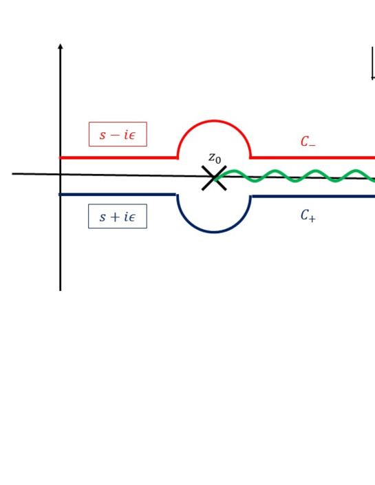
Fig. 4: Integration contours $C_{+}$ and $C_{-}$ on the Borel plane.

We identify an ambiguity as difference between them:

$$\text{Amb.}\,u_{\alpha}(s)\equiv u_{\alpha}(s+i\epsilon)-u_{\alpha}(s-i\epsilon)=\int_{C_{+}}dz\,e^{-z}\left(1-\frac{z^{2}}{z_{0}^{2}}\right)^{\alpha}-\int_{C_{-}}dz\,e^{-z}\left(1-\frac{z^{2}}{z_{0}^{2}}\right)^{\alpha}$$

$$= 2i\sin(\alpha\pi)\int_{z_{0}}^{\infty}dz\,e^{-z}\left(\frac{z^{2}}{z_{0}^{2}}-1\right)^{\alpha}$$

$$= \frac{i}{\sqrt{\pi}}\sin(\alpha\pi)\frac{3^{\alpha-\frac{1}{2}}}{2^{\alpha-\frac{5}{2}}}s^{-\frac{3}{2}\left(\alpha-\frac{1}{2}\right)}\Gamma(\alpha+1)K_{\alpha+\frac{1}{2}}(z_{0})$$

$$\sim 2i\sin(\alpha\pi)\Gamma(\alpha+1)\left(\frac{3}{2}\right)^{\alpha}s^{-\frac{3}{2}\alpha}e^{-\frac{4}{3}s^{\frac{3}{2}}}\left(1+\frac{3}{8}\alpha(\alpha+1)s^{-\frac{3}{2}}+{\cal O}(s^{-3})\right),$$ (4.58)

where we have used the asymptotic form of the modified Bessel function. Important observation here is that $\text{Amb.}\,u_{\alpha}(s)$ with the smallest $\alpha$ becomes the most dominant in the large-$s$ regime. Hence picking up the smallest power of $\left(1-\frac{z^{2}}{z_{0}^{2}}\right)$ in (4.54), we find

$$\text{Amb.}\int_{0}^{\infty}dz\,e^{-z}T_{pq}(z)\sim -\frac{\pi^{\frac{3}{2}}}{2\cdot 3^{\frac{p}{2}+1}}\sum_{j=0}^{\frac{q-1}{2}}\left(-\frac{1}{3}\right)^{j}\frac{\Gamma\left(-j-\frac{1}{2}\right)}{\Gamma\left(-j+\frac{q+1}{2}\right)}\frac{1}{\Gamma\left(j+\frac{p}{2}+2\right)}$$

$$\times b_{j}^{(j)}\left(j+\frac{p}{2}+1\right)(-1)^{j}\,\text{Amb.}\,u_{\frac{p}{2}+1}(s)\left(1+{\cal O}\left(s^{-\frac{3}{2}}\right)\right).$$ (4.59)

Finally we use the result shown in appendix B

$$b_{j}^{(j)}(\alpha)=-\frac{3^{j}}{2\sqrt{\pi}}\frac{\Gamma(\alpha+1)}{\Gamma(\alpha+1-j)},$$ (4.60)

and then from (4.46), we obtain

$$\text{Amb.}\,N^{\frac{p+q}{3}+2}\left.\left\langle\frac{1}{N}\text{tr}\,\phi^{p}\frac{1}{N}\text{tr}\,\phi^{q}\right\rangle_{c}^{(1,0)}\right|_{\text{0-inst., univ.}}$$

$$=i\sin\left(\frac{p}{2}\pi\right)\frac{1}{2^{\frac{p}{2}+2}\pi^{\frac{5}{2}}q}\Gamma\left(\frac{p}{2}+1\right)\frac{\Gamma\left(\frac{q}{2}+1\right)}{\Gamma\left(\frac{q+1}{2}\right)}s^{-\frac{p}{4}+\frac{q}{2}-\frac{3}{2}}e^{-\frac{4}{3}s^{\frac{3}{2}}}\ln s\left(1+{\cal O}(s^{-\frac{3}{2}})\right)+(p\leftrightarrow q),$$ (4.61)

where the sum on $j$ is taken as

$$\sum_{j=0}^{\frac{q-1}{2}}\frac{\Gamma\left(-j-\frac{1}{2}\right)}{\Gamma\left(-j+\frac{q+1}{2}\right)}=-\frac{2\sqrt{\pi}}{q\Gamma\left(\frac{q+1}{2}\right)}.$$ (4.62)

The above derivation implies that all $j$’s in the sum in (4.34) contribute to the leading order in the ambiguity. Without loss of generality we can assume $p\leq q$ and then (4.61) leads to

$$\text{Amb.}\,N^{\frac{p+q}{3}+2}\left.\left\langle\frac{1}{N}\text{tr}\,\phi^{p}\frac{1}{N}\text{tr}\,\phi^{q}\right\rangle_{c}^{(1,0)}\right|_{\text{0-inst., univ.}}$$

$$=i(1+\delta_{pq})\sin\left(\frac{p}{2}\pi\right)\frac{1}{2^{\frac{p}{2}+2}\pi^{\frac{5}{2}}q}\Gamma\left(\frac{p}{2}+1\right)\frac{\Gamma\left(\frac{q}{2}+1\right)}{\Gamma\left(\frac{q+1}{2}\right)}s^{-\frac{p}{4}+\frac{q}{2}-\frac{3}{2}}e^{-\frac{4}{3}s^{\frac{3}{2}}}\ln s\left(1+{\cal O}(s^{-\frac{3}{2}})\right).$$ (4.63)

As in (2.14) it is shown that weight of the one-instanton in our matrix model is proportional to $e^{-\frac{4}{3}s^{\frac{3}{2}}}$ and, therefore, it is likely that the ambiguity in the zero-instanton sector in (4.63) would be canceled by another ambiguity in the one-instanton sector according to resurgence. We will confirm this in the next section.

5 Two-point function in the one-instanton sector

In the previous section, we derived the perturbative series of the two-point function of the odd operators under the double scaling limit. We found that it is non-Borel summable and gave the explicit form of its ambiguity at the leading order of the large-$s$ regime. In this section we consider the two-point function in the one-instanton sector and show that it also has ambiguity, which exactly cancels that in the zero-instanton sector at the leading order in the large-$s$ regime. Thus we confirm that resurgence works in the two-point functions.

5.1 Review of two-point function in the random matrix theory

As in (4.2), the two-point function in our model can be deduced from that in the Gaussian matrix model, where a nice formula for the two-point function has been already known in the literature. Hence we review it in the context of the Gaussian Unitary Ensemble (GUE).

The GUE is defined in terms of the partition function

$$Z^{(G)}\equiv\int dM\,e^{-\frac{N}{2}\text{tr}\,M^{2}}=\tilde{C}_{N}\int_{-\infty}^{\infty}\prod_{i=1}^{N}dx_{i}\,\Delta(x)^{2}\,e^{-N\sum_{i}\frac{1}{2}x_{i}^{2}},$$ (5.1)

where $M$ is an $N\times N$ Hermitian matrix and $x_{i}$ ($i=1,\cdots,M$) are its eigenvalues. Note that in this section we discuss the standard GUE in (5.1), which is different from the one in (3.6) with the upper bound for $x_{i}$ we have already discussed. Associated with (5.1), a joint probability distribution is defined as

$$P(\{x\})\equiv\frac{\tilde{C}_{N}}{Z^{(G)}}\Delta(x)^{2}\,e^{-N\sum_{i}\frac{1}{2}x_{i}^{2}},$$ (5.2)

then

$$\int\prod_{i=1}^{N}dx_{i}\,P({\{x\}})=1.$$ (5.3)

The two-point function, or covariance in the GUE is given as

$$\left\langle\frac{1}{N}\text{tr}\,f(M)\frac{1}{N}\text{tr}\,g(M)\right\rangle^{(G)}=\frac{1}{Z^{(G)}}\int dM\,\frac{1}{N}\text{tr}\,f(M)\frac{1}{N}\text{tr}\,g(M)\,e^{-\frac{N}{2}\text{tr}\,M^{2}}$$

$$=\frac{\tilde{C}_{N}}{Z^{(G)}}\int_{-\infty}^{\infty}\prod_{i=1}^{N}dx_{i}\,\Delta(x)^{2}\frac{1}{N^{2}}\sum_{i,j=1}^{N}f(x_{i})g(x_{j})\,e^{-N\sum_{i}\frac{1}{2}x_{i}^{2}}$$

$$=\frac{\tilde{C}_{N}}{Z^{(G)}}\int_{-\infty}^{\infty}\prod_{i=1}^{N}dx_{i}\,\Delta(x)^{2}\frac{1}{N^{2}}(Nf(x_{1})g(x_{1})+N(N-1)f(x_{1})g(x_{2}))\,e^{-N\sum_{i}\frac{1}{2}x_{i}^{2}}.$$ (5.4)

Introducing the $k$-point correlation function obtained by integrating $P(\{x\})$ with respect to $N-k$ variables

$$R_{k}(x_{1},\cdots,x_{k})\equiv\frac{N!}{(N-k)!}\int_{-\infty}^{\infty}\prod_{i=k+1}^{N}dx_{i}\,P(\{x\}),$$ (5.5)

the two-point function becomes

$$\left\langle\frac{1}{N}\text{tr}\,f(M)\frac{1}{N}\text{tr}\,g(M)\right\rangle^{(G)}$$

$$=\frac{1}{N^{2}}\int_{-\infty}^{\infty}dx\,f(x)g(x)R_{1}(x)+\frac{1}{N^{2}}\int_{-\infty}^{\infty}dxdy\,f(x)g(y)R_{2}(x,y).$$ (5.6)

Now an important role is played by a kernel

$$K(x,y)= e^{-\frac{N}{4}\left(x^{2}+y^{2}\right)}\sum_{n=0}^{N-1}\frac{1}{h_{n}}p_{n}(x)p_{n}(y)$$

$$= e^{-\frac{N}{4}\left(x^{2}+y^{2}\right)}\frac{1}{h_{N-1}}\frac{p_{N}(x)p_{N-1}(y)-p_{N-1}(x)p_{N}(y)}{x-y},$$ (5.7)

where $p_{n}(x)$ ($n=0,\cdots,N-1$) is a monic orthogonal polynomial of degree $n$ satisfying

$$\int_{-\infty}^{\infty}dx\,e^{-\frac{N}{2}x^{2}}p_{m}(x)p_{n}(y)=h_{n}\delta_{mn}.$$ (5.8)

More precisely,

$$p_{n}(x)=\frac{1}{(2N)^{\frac{n}{2}}}H_{n}\left(\sqrt{\frac{N}{2}}x\right),\qquad\text{with}\quad H_{n}(x)=(-1)^{n}e^{x^{2}}\frac{d^{n}}{dx^{n}}e^{-x^{2}},$$

$$h_{n}=\frac{\sqrt{2\pi}n!}{N^{n+\frac{1}{2}}}.$$ (5.9)

The kernel is related to the one-point and two-point functions as

$$R_{1}(x)=K(x,x)=N\rho(x),\qquad\text{with}\quad\rho(x)=\left\langle\frac{1}{N}\delta(x-M)\right\rangle^{(G)},$$

$$R_{2}(x,y)=K(x,x)K(y,y)-K(x,y)^{2}.$$ (5.10)

Substituting these equations for (5.6) yields

$$\left\langle\frac{1}{N}\text{tr}\,f(M)\frac{1}{N}\text{tr}\,g(M)\right\rangle^{(G)}=\left\langle\frac{1}{N}\text{tr}\,f(M)g(M)\right\rangle^{(G)}$$

$$+\left\langle\frac{1}{N}\text{tr}\,f(M)\right\rangle^{(G)}\left\langle\frac{1}{N}\text{tr}\,g(M)\right\rangle^{(G)}-\frac{1}{N^{2}}\int_{-\infty}^{\infty}dxdy\,f(x)g(y)K(x,y)^{2}.$$ (5.11)

Therefore,

$$\left\langle\frac{1}{N}\text{tr}\,f(M)\frac{1}{N}\text{tr}\,g(M)\right\rangle^{(G)}_{c}=\left\langle\frac{1}{N}\text{tr}\,f(M)g(M)\right\rangle^{(G)}-\frac{1}{N^{2}}\int_{-\infty}^{\infty}dxdy\,f(x)g(y)K(x,y)^{2}.$$ (5.12)

5.2 Application to our model

In our model, as in (3.5), the two-point function of odd operators in the filling fraction $(1,0)$ is expressed via the Nicolai mapping as

$$\left\langle\frac{1}{N}\text{tr}\,\phi^{p}\frac{1}{N}\text{tr}\,\phi^{q}\right\rangle^{(1,0)}= \frac{\tilde{C}_{N}}{Z_{(1,0)}}\int_{0}^{\infty}\prod_{k=1}^{N}\left(2\lambda_{k}d\lambda_{k}\right)\Delta(\lambda^{2})^{2}\frac{1}{N^{2}}\sum_{i,j=1}^{N}\lambda_{i}^{p}\lambda_{j}^{q}\,e^{-\frac{N}{2}\sum_{k}(\lambda_{k}^{2}-\mu^{2})^{2}}$$

$$= \frac{\tilde{C}_{N}}{Z_{(1,0)}}\int_{-\infty}^{\mu^{2}}\prod_{k=1}^{N}dx_{k}\,\Delta(x)^{2}\frac{1}{N^{2}}\sum_{i,j=1}^{N}(\mu^{2}-x_{i})^{\frac{p}{2}}(\mu^{2}-x_{j})^{\frac{q}{2}}\,e^{-\frac{N}{2}\sum_{k}x_{k}^{2}}$$

$$= \left\langle\frac{1}{N}\text{tr}\,(\mu^{2}-M)^{\frac{p}{2}}\frac{1}{N}\text{tr}\,(\mu^{2}-M)^{\frac{q}{2}}\right\rangle^{(G^{\prime})},$$ (5.13)

where $(G^{\prime})$ indicates that $x_{i}$ integration has upper boundary $x_{i}=\mu^{2}$ as in (3.6). Since (5.10) follows from existence of the orthogonal polynomials, in the GUE with the boundary we also have a formula of the two-point function similar to (5.12):

$$\left\langle\frac{1}{N}\text{tr}\,f(M)\frac{1}{N}\text{tr}\,g(M)\right\rangle^{(G^{\prime})}_{c}=\left\langle\frac{1}{N}\text{tr}\,f(M)g(M)\right\rangle^{(G^{\prime})}-\frac{1}{N^{2}}\int_{-\infty}^{\mu^{2}}dxdy\,f(x)g(y)K^{(G^{\prime})}(x,y)^{2},$$ (5.14)

where $K^{(G^{\prime})}(x,y)$ is the kernel of the GUE with the boundary. However, as far as the zero- and one-instanton contribution is concerned, we can replace $K^{(G^{\prime})}(x,y)$ with $K(x,y)$ in the standard GUE in (5.7). In fact, the kernel $K^{(G^{\prime})}(x,y)$ in the GUE with the boundary is also given as in (5.7)

$$K^{(G^{\prime})}(x,y)= e^{-\frac{N}{4}\left(x^{2}+y^{2}\right)}\frac{1}{h_{N-1}^{(G^{\prime})}}\frac{p_{N}^{(G^{\prime})}(x)p^{(G^{\prime})}_{N-1}(y)-p^{(G^{\prime})}_{N-1}(x)p_{N}^{(G^{\prime})}(y)}{x-y},$$ (5.15)

where $p_{N}^{(G^{\prime})}$ is the orthogonal polynomial in the presence of the boundary

$$\int_{-\infty}^{\mu^{2}}dx\,e^{-\frac{N}{2}x^{2}}p_{m}^{(G^{\prime})}(x)p_{n}^{(G^{\prime})}(y)=h_{n}^{(G^{\prime})}\delta_{mn}.$$ (5.16)

In [55] we explicitly demonstrate that differences are expanded as

$$\tilde{p}_{n}(x)\equiv p_{n}^{(G^{\prime})}(x)-p_{n}(x)=\tilde{p}_{n}^{(1)}(x)+\tilde{p}_{n}^{(2)}(x)+\cdots,$$

$$\tilde{h}_{n}\equiv h_{n}^{(G^{\prime})}-h_{n}=\tilde{h}_{n}^{(1)}+\tilde{h}_{n}^{(2)}+\cdots$$ (5.17)

by taking account of the boundary effect iteratively and this expansion turns out to be in terms of the instanton number. Then difference of the kernel is written as

$$\tilde{K}(x,y)\equiv K^{(G^{\prime})}(x,y)-K(x,y)=\tilde{K}^{(1)}(x,y)+\tilde{K}^{(2)}(x,y)+\cdots,$$

$$\tilde{K}^{(1)}(x,y)$$

$$=e^{-\frac{N}{4}(x^{2}+y^{2})}\frac{1}{x-y}\Biggl{\{}\frac{1}{h_{N-1}}\left(\tilde{L}_{N}^{(1)}(x)+\tilde{L}_{N-1}^{(1)}(y)-\frac{\tilde{h}_{N-1}^{(1)}}{h_{N-1}}\right)p_{N}(x)p_{N-1}(y)-(x\leftrightarrow y)\Biggr{\}},$$ (5.18)

where

$$\tilde{L}_{n}(x)\equiv\frac{p_{n}^{(G^{\prime})}(x)}{p_{n}(x)}=\tilde{L}_{n}^{(1)}(x)+\tilde{L}_{n}^{(2)}(x)+\cdots.$$ (5.19)

Since later we will find that the second term in (5.14) is relevant for ambiguity in the one-instanton sector, we need to evaluate

$$\int_{-\infty}^{\mu^{2}}dxdy\,f(x)g(y)\tilde{K}^{(1)}(x,y)^{2}.$$ (5.20)

By using the results in [55], it is not difficult to see that the integrations on $x$ and $y$ are dominated by $x=y$ configuration. In fact, since it is shown in [55] that $\tilde{L}_{N}^{(1)}(x)=L(x,1)S_{N}^{(1)}$ where $L(x,1)$ is a function of ${\cal O}(N^{0})$ and $S_{N}$ is an $N$-dependent constant, $x,y$-dependence of $K^{(1)}(x,y)$ is essentially the same. More precisely, $e^{-\frac{x^{2}}{4}}p_{n}(x)$ takes a form of $e^{-\frac{x^{2}}{4}}p_{n}(x)\propto\exp(-Nf_{n}(x))(1+{\cal O}(1/N))$ with a function $f_{n}(x)$ of ${\cal O}(N^{0})$, and hence the saddle points of $x$ and $y$ integrations become the same in the large-$N$ limit, and as a consequence, we need to take $y\rightarrow x$ limit. Then the problem is reduced to the one-point function by (5.10). However, as mentioned in [54], in the case of the one-point function,

$$\int_{-\infty}^{\mu^{2}}dx\,(\mu^{2}-x)^{n}\tilde{\rho}^{(1)}(x)$$ (5.21)

is shown to have $p\geq 2-$instanton weight. Thus in (5.13) we restrict ourselves to up to the one-instanton sector, and by using (5.14) and replacing $K^{(G^{\prime})}(x,y)$ with $K(x,y)$, we obtain

$$\left.\left\langle\frac{1}{N}\text{tr}\,\phi^{p}\frac{1}{N}\text{tr}\,\phi^{q}\right\rangle^{(1,0)}_{c}\right|_{\text{0-inst.}+\text{1-inst.}}= \left.\left\langle\frac{1}{N}\text{tr}\,(\mu^{2}-M)^{\frac{p+q}{2}}\right\rangle^{(G^{\prime})}\right|_{\text{0-inst.}+\text{1-inst.}}$$

$$-\frac{1}{N^{2}}\left.\int_{-\infty}^{\mu^{2}}dxdy\,(\mu^{2}-x)^{\frac{p}{2}}(\mu^{2}-y)^{\frac{q}{2}}K(x,y)^{2}\right|_{\text{0-inst.}+\text{1-inst.}}.$$ (5.22)

When both $p$ and $q$ are odd, the first term on the right-hand side is the regular one-point function and has no ambiguity. Hence we concentrate on the second term

$$G_{pq}\equiv\left.-\frac{1}{N^{2}}\int_{-\infty}^{\mu^{2}}dxdy\,(\mu^{2}-x)^{\frac{p}{2}}(\mu^{2}-y)^{\frac{q}{2}}K(x,y)^{2}\right|_{\text{0-inst.}+\text{1-inst.}}$$ (5.23)

and examine whether it has ambiguity.

Since we are interested in $G_{pq}$ in the double scaling limit, we set

$$\mu^{2}=2+N^{-\frac{2}{3}}s,\quad x=2+N^{-\frac{2}{3}}\xi,\quad y=2+N^{-\frac{2}{3}}\eta.$$ (5.24)

This limit corresponds to the soft edge scaling limit in the random matrix theory, under which the kernel in the GUE becomes the Airy kernel:

$$\lim_{N\rightarrow\infty}N^{-\frac{2}{3}}K(2+N^{-\frac{2}{3}}\xi,2+N^{-\frac{2}{3}}\eta)=K_{\text{Ai}}(\xi,\eta),$$

$$K_{\text{Ai}}(\xi,\eta)\equiv\frac{\text{Ai}(\xi)\text{Ai}^{\prime}(\eta)-\text{Ai}^{\prime}(\xi)\text{Ai}(\eta)}{\xi-\eta},$$ (5.25)

and then $G_{pq}$ is given by

$$G_{pq}=-N^{-\frac{p+q}{3}-2}\int_{-\infty}^{s}d\xi d\eta\,(s-\xi)^{\frac{p}{2}}(s-\eta)^{\frac{q}{2}}K_{\text{Ai}}(\xi,\eta)^{2}.$$ (5.26)

Let us consider $G_{pq}$ in the one-instanton sector. According to (2.13), the integrations on $\lambda_{i}$ and $\lambda_{j}$ on the right-hand side in the first line in (5.13) are now restricted as

$$\int_{0}^{a}2\lambda_{i}d\lambda_{i}\int_{a}^{b}2\lambda_{j}d\lambda_{j}\cdot+\int_{a}^{b}2\lambda_{i}d\lambda_{i}\int_{0}^{a}2\lambda_{j}d\lambda_{j}\cdot,$$ (5.27)

which becomes via the Nicolai mapping $x=\mu^{2}-\lambda_{i}^{2}$, $y=\mu^{2}-\lambda_{j}^{2}$, and (5.24),

$$N^{-\frac{4}{3}}\int_{0}^{s}d\xi\int_{-\infty}^{0}d\eta\,\cdot+N^{-\frac{4}{3}}\int_{-\infty}^{0}d\xi\int_{0}^{s}d\eta\,\cdot.$$ (5.28)

Namely one of the integrations are in the perturbative region and the other in the nonperturbative region. Therefore,

$$\left.N^{\frac{p+q}{3}+2}G_{pq}\right|_{\text{1-inst.}}= -\left(\int_{0}^{s}d\xi\int_{-\infty}^{0}d\eta+\int_{-\infty}^{0}d\xi\int_{0}^{s}d\eta\right)(s-\xi)^{\frac{p}{2}}(s-\eta)^{\frac{q}{2}}K_{\text{Ai}}(\xi,\eta)^{2}$$

$$= -\int_{0}^{s}d\xi\int_{-\infty}^{0}d\eta\,(s-\xi)^{\frac{p}{2}}(s-\eta)^{\frac{q}{2}}K_{\text{Ai}}(\xi,\eta)^{2}+(p\leftrightarrow q).$$ (5.29)

Let us consider the first term where $\xi\in[0,s]$ and $\eta\in(-\infty,0]$. Since later it turns out that relevant contribution comes from $\xi\sim s\gg 1$ and $|\eta|\gg 1$, we use the asymptotic form of the Airy function in the Airy kernel

$$\text{Ai}(\xi)\sim\frac{e^{-z}}{2\sqrt{\pi}\xi^{\frac{1}{4}}}\left(u_{e}(z)+u_{o}(z)\right)\qquad(\xi\gg 1),$$ (5.30)

$$\text{Ai}(\eta)\sim\frac{1}{\sqrt{\pi}|\eta|^{\frac{1}{4}}}\left(\cos\left(w-\frac{\pi}{4}\right)u_{e}(w)+\sin\left(w-\frac{\pi}{4}\right)u_{o}(w)\right)\qquad(-\eta\gg 1),$$ (5.31)

where

$$z\equiv\frac{2}{3}\xi^{\frac{3}{2}},\qquad w\equiv\frac{2}{3}|\eta|^{\frac{3}{2}},$$ (5.32)

and

$$u_{e}(z)=\sum_{k=0}^{\infty}(-1)^{k}\frac{u_{2k}}{z^{2k}},\qquad u_{o}(z)=\sum_{k=0}^{\infty}(-1)^{k}\frac{u_{2k+1}}{z^{2k+1}},$$

$$u_{k}=\frac{(2k+1)(2k+3)\cdots(6k-1)}{216^{k}\,k!}.$$ (5.33)

Plugging these into $K_{\text{Ai}}(\xi,\eta)$ in (5.25), it is rewritten for $\xi\gg 1$, $-\eta\gg 1$ as

$$(\xi-\eta)K_{\text{Ai}}(\xi,\eta)$$

$$=\frac{e^{-z}}{2\pi\xi^{\frac{1}{4}}|\eta|^{\frac{1}{4}}}\Biggl{(} \sin\left(w-\frac{\pi}{4}\right)\left(|\eta|^{\frac{1}{2}}(u_{e}(z)+u_{o}(z))v_{e}(w)+\xi^{\frac{1}{2}}(v_{e}(z)+v_{o}(z))u_{o}(w)\right)$$

$$+ \cos\left(w-\frac{\pi}{4}\right)\left(-|\eta|^{\frac{1}{2}}(u_{e}(z)+u_{o}(z))v_{o}(w)+\xi^{\frac{1}{2}}(v_{e}(z)+v_{o}(z))u_{e}(w)\right)\Biggr{)},$$ (5.34)

where

$$v_{e}(z)=\sum_{k=0}^{\infty}(-1)^{k}\frac{v_{2k}}{z^{2k}},\qquad v_{o}(z)=\sum_{k=0}^{\infty}(-1)^{k}\frac{v_{2k+1}}{z^{2k+1}},$$

$$v_{k}=\frac{6k+1}{1-6k}u_{k}.$$ (5.35)

5.3 Saddle point method

In the presence of $e^{-z}$ in (5.34), we first apply the saddle point method to the integration on $\xi$ in the first term in (5.29). We define $f(\xi,\eta)$ by

$$\left.N^{\frac{p+q}{3}+2}G_{pq}\right|_{\text{1-inst.}}\equiv-\int_{0}^{s}d\xi\int_{-\infty}^{0}d\eta\,e^{-f(\xi,\eta)}+(p\leftrightarrow q),$$ (5.36)

then

$$f(\xi,\eta)= 2z-\frac{p}{2}\ln(s-\xi)-\frac{q}{2}\ln(s-\eta)+2\ln(\xi-\eta)-\frac{1}{2}\ln\xi+\frac{1}{2}\ln|\eta|+2\ln(2\pi)$$

$$-2\ln\Biggl{\{}\left(\frac{|\eta|}{\xi}\right)^{\frac{1}{2}}\left(\sin\left(w-\frac{\pi}{4}\right)-\frac{3}{2}\cos\left(w-\frac{\pi}{4}\right)v_{1}|\eta|^{-\frac{3}{2}}\right)$$

$$\phantom{-2\ln\Biggl{\{}\left(\frac{|\eta|}{\xi}\right)^{\frac{1}{2}}}+\cos\left(w-\frac{\pi}{4}\right)+\frac{3}{2}\sin\left(w-\frac{\pi}{4}\right)u_{1}|\eta|^{-\frac{3}{2}}\Biggr{\}}$$

$$\times\left(1+{\cal O}(\xi^{-\frac{3}{2}})\right)\left(1+{\cal O}(\eta^{-3})\right).$$ (5.37)

We will find later that $|\eta|$ becomes ${\cal O}(s)$ and hence we have to retain $\left(\frac{|\eta|}{\xi}\right)^{\frac{1}{2}}$ term. From this definition, a saddle point with respect to $\xi$: $\partial_{\xi}f(\xi_{*},\eta)=0$ is near $\xi=s$ as

$$\xi_{*}=s+\frac{p}{4s^{\frac{1}{2}}}+{\cal O}(s^{-2}).$$ (5.38)

This justifies the use of the asymptotic formula of the Airy function for $\xi\gg 1$ in (5.30). Here we note that since $\eta\in(-\infty,0]$, $\frac{1}{\xi_{*}-\eta}\leq\frac{1}{\xi_{*}}$ and it is at most of ${\cal O}(s^{-1})$. We also have

$$\partial_{\xi}^{2}f(\xi_{*},\eta)=\frac{8s}{p}+\frac{3(p+4)}{p}s^{-\frac{1}{2}}+{\cal O}(s^{-2}),$$

$$\partial_{\xi}^{n}f(\xi_{*},\eta)=\frac{p}{2}\Gamma(n)\left(-\frac{4s^{\frac{1}{2}}}{p}\right)^{n}\left(1+\frac{n(p+6)}{8}s^{-\frac{3}{2}}+{\cal O}(s^{-3})\right)\qquad(n\geq 3).$$ (5.39)

We recognize here that even if $\partial_{\xi}^{2}f(\xi_{*},\eta)$ is of ${\cal O}(s)$, we have to take account of all order in the Gaussian approximation because $\partial_{\xi}^{n}f(\xi_{*},\eta)$ is of ${\cal O}(s^{\frac{n}{2}})$. Using these equations, the Taylor expansion of $f(\xi,\eta)$ around $\xi=\xi_{*}$ reads

$$f(\xi,\eta)=f(\xi_{*},\eta)+\frac{1}{2}\partial_{\xi}^{2}f(\xi_{*},\eta)(\xi-\xi_{*})^{2}+\sum_{n=3}^{\infty}\frac{1}{n!}\partial_{\xi}^{n}f(\xi_{*},\eta)(\xi-\xi_{*})^{n}$$

$$=f(\xi_{*},\eta)+2s^{\frac{1}{2}}(\xi-\xi_{*})+\frac{3(p+4)}{2p}s^{-\frac{1}{2}}(\xi-\xi_{*})^{2}-\frac{p}{2}\ln\left(1+\frac{4s^{\frac{1}{2}}}{p}(\xi-\xi_{*})\right)+{\cal O}(s^{-2}).$$ (5.40)

By setting

$$t=2s^{\frac{1}{2}}(\xi-\xi_{*}),$$ (5.41)

the integration on $\xi$ becomes

$$\int d\xi\,e^{-f(\xi,\eta)}=e^{-f(\xi_{*},\eta)}\frac{1}{2s^{\frac{1}{2}}}\int dt\,e^{-t}\left(1+\frac{2t}{p}\right)^{\frac{p}{2}}(1+{\cal O}(s^{-\frac{3}{2}})).$$ (5.42)

Now let us consider the integration contour. In performing the integration on $\xi$ in (5.36), we find that the saddle point in (5.38) is not in the integration region. Here we follow the prescription proposed in [54]. Namely, we rotate the integration contour $[0,s]$ by $\pm\pi$ around the branch point $\xi=s$ so that it will pass through the saddle point $\xi=\xi_{*}$ without going through any singularity. More precisely, in order to avoid the cut $[s,\infty)$ of $\ln(s-\xi)$ in (5.37), we have to make the rotation by $\pm\pi$ for $s\rightarrow s\pm i\epsilon$ with $\epsilon>0$. Thus the contour becomes a one on the positive real axis in the opposite direction decreasing $\xi$, and terminating at $\xi=s$. From the definition of $t$ in (5.41), we zoom in the vicinity of the saddle point in the large-$s$ regime and hence the lower limit of the integration (after $\pm\pi$ rotation) is $+\infty$ as usual in the standard saddle point method. On the other hand, even for the variable $t$, the upper edge $\xi=s$ remains finite $t=-\frac{p}{2}+{\cal O}(s^{-\frac{3}{2}})$ due to $\eqref{eq:xi*}$ and (5.41). Thus in this prescription the $\xi$ integration can be performed as

$$\int d\xi\,e^{-f(\xi,\eta)}= e^{-f(\xi_{*},\eta)}\frac{1}{2s^{\frac{1}{2}}}\int_{\infty}^{-\frac{p}{2}}dt\,e^{-t}\left(1+\frac{2t}{p}\right)^{\frac{p}{2}}(1+{\cal O}(s^{-\frac{3}{2}}))$$

$$= -e^{-f(\xi_{*},\eta)}\left(\frac{2}{p}\right)^{\frac{p}{2}}e^{\frac{p}{2}}\frac{1}{2s^{\frac{1}{2}}}\Gamma\left(\frac{p}{2}+1\right)(1+{\cal O}(s^{-\frac{3}{2}})).$$ (5.43)

The steepest descent method by choosing the contour passing through the saddle point in this way should provide the trans-series in the one-instanton sector. In fact, in [54] it is shown that in the case of the one-point function, this prescription works and we can check explicitly the resurgence under it. It should be noticed that as mentioned in [54], the rotations of the contour by $\pm\pi$ according to $s\rightarrow s\pm i\epsilon$ give the same integrand and do not cause any difference. Thus so far there is no ambiguity between $s\rightarrow s\pm i\epsilon$. It is in fact the saddle point value $f(\xi_{*},\eta)$ that makes difference. This situation is also the same as in the case of the one-point function [54]. The origin of ambiguity is, under $s\to s\pm i\epsilon$,

$$\ln(s-\xi_{*})\rightarrow\ln(s\pm i\epsilon-\xi_{*})=\ln(\xi_{*}-s)\pm i\pi.$$ (5.44)

Plugging the saddle point $\eqref{eq:xi*}$ into (5.37) and using (5.43) and (5.44), we get

$$\left.N^{\frac{p+q}{3}+2}G_{pq}\right|_{\text{1-inst.}}$$

$$=e^{\pm\frac{p}{2}\pi i}\frac{1}{2^{\frac{p}{2}+3}\pi^{2}}\Gamma\left(\frac{p}{2}+1\right)s^{-\frac{p}{4}}e^{-\frac{4}{3}s^{\frac{3}{2}}}(1+{\cal O}(s^{-\frac{3}{2}}))$$

$$\times\int_{-\infty}^{0}d\eta\,\frac{1}{|\eta|^{\frac{1}{2}}}(s-\eta)^{\frac{q}{2}-2}\Bigg{\{}|\eta|^{\frac{1}{2}}s^{-\frac{1}{2}}\left(\sin\left(w-\frac{\pi}{4}\right)-\frac{3}{2}\cos\left(w-\frac{\pi}{4}\right)v_{1}|\eta|^{-\frac{3}{2}}\right)$$

$$\phantom{\times\int_{-\infty}^{0}d\eta\,\frac{1}{|\eta|^{\frac{1}{2}}}(s-\eta)^{\frac{q}{2}-2}|\eta|^{\frac{1}{2}}s^{-\frac{1}{2}}}+\left(\cos\left(w-\frac{\pi}{4}\right)+\frac{3}{2}\sin\left(w-\frac{\pi}{4}\right)u_{1}|\eta|^{-\frac{3}{2}}\right)\Biggr{\}}^{2}(1+{\cal O}(\eta^{-3}))$$

$$+(p\leftrightarrow q).$$ (5.45)

5.4 Contribution from perturbative region

Finally let us consider the $\eta$-integration. From (5.45), it reads

$$I_{\eta} \equiv\int_{0}^{\infty}d\eta\,\frac{1}{\eta^{\frac{1}{2}}}(s+\eta)^{\frac{q}{2}-2}$$

$$\times\biggl{\{}\sin\left(w-\frac{\pi}{4}\right)\left(\eta^{\frac{1}{2}}s^{-\frac{1}{2}}+\frac{3}{2}u_{1}\eta^{-\frac{3}{2}}\right)+\cos\left(w-\frac{\pi}{4}\right)\left(1-\frac{3}{2}v_{1}s^{-\frac{1}{2}}\eta^{-1}\right)\biggr{\}}^{2}(1+{\cal O}(\eta^{-3})).$$ (5.46)

Expansion of the curly braces yields both oscillating terms with $\sin(2w)$, $\cos(2w)$, and non-oscillating one. Since $\eta\gg 1$ contribution is relevant for the integration, we anticipate that the former ones oscillate quite rapidly and their integrals vanish. For this reason we assume that they do not contribute and simply drop them. In fact, this prescription enables us to compute the one-point function at higher genus via the Airy kernel $K_{\text{Ai}}(\xi,\xi)$, which exactly reproduces the result derived by another method in [53]. The prescription becomes necessary because we take the double scaling limit at the level of the integrand from (5.23) to (5.26). Originally the kernel consists of the orthogonal polynomials as in (5.15) and in the double scaling limit they have the oscillating behavior. If we were able to take the double scaling limit after the integration on $x$ and $y$ in (5.23), we would not have to make such an assumption. Then the integration on $\eta$ are simplified as

$$I_{\eta}=\frac{1}{2}\int_{0}^{\infty}d\eta\,\left(\frac{1}{s}\eta^{\frac{1}{2}}(s+\eta)^{\frac{q}{2}-2}+\eta^{-\frac{1}{2}}(s+\eta)^{\frac{q}{2}-2}\right)\left(1+{\cal O}(s^{-\frac{1}{2}}\eta^{-1},\eta^{-\frac{3}{2}})\right).$$ (5.47)

Since we are now computing the integration with respect to the one variable in the perturbative region, it is natural to expect that it is related to a quantity in the one-point function. In fact, from the definition (4.24), it is easy to see that the integrals above can be written in terms of $I_{m,n}$ as, for odd $m$,

$$\int_{0}^{\infty}d\xi\,\xi^{\frac{m}{2}}(s+\xi)^{\frac{n}{2}}=\left(N^{-\frac{2}{3}}\right)^{-\frac{m+n}{3}-1}\pi i\left(\frac{i}{2}\right)^{m}I_{m,n}.$$ (5.48)

Hence from (LABEL:eq:Iresult),

$$\left.I_{\eta}\right|_{\text{univ.}}=\frac{1}{2}\left(s^{-1}I_{1,q-4}+I_{-1,q-4}\right)=-\frac{1}{2\sqrt{\pi}}\frac{\Gamma\left(\frac{q}{2}\right)}{\Gamma\left(\frac{q+1}{2}\right)}s^{\frac{q-3}{2}}\ln s\,(1+{\cal O}(s^{-\frac{3}{2}})).$$ (5.49)

Now it becomes clear why we keep $\left(\frac{|\eta|}{\xi}\right)^{\frac{1}{2}}$ term in (5.37). In fact, the saddle point of $\xi$ is of ${\cal O}(s)$ as in (5.38), while the power of $\eta$ increases the power of $s$ according to (LABEL:eq:Iresult). Substituting this for (5.45), we find

$$\left.N^{\frac{p+q}{3}+2}G_{pq}\right|_{\text{1-inst., univ.}}= -e^{\pm\frac{p}{2}\pi i}\frac{1}{2^{\frac{p}{2}+4}\pi^{\frac{5}{2}}}\Gamma\left(\frac{p}{2}+1\right)\frac{\Gamma\left(\frac{q}{2}\right)}{\Gamma\left(\frac{q+1}{2}\right)}s^{-\frac{p}{4}+\frac{q}{2}-\frac{3}{2}}e^{-\frac{4}{3}s^{\frac{3}{2}}}\ln s\,(1+{\cal O}(s^{-\frac{3}{2}}))$$

$$+(p\leftrightarrow q).$$ (5.50)

Thus if we assume $p\leq q$ as in (4.63), the first term is more leading on the right-hand side in this equation. Therefore, the ambiguity in the two-point function in the one-instanton sector is

$$\text{Amb.}\,N^{\frac{p+q}{3}+2}\left.\left\langle\frac{1}{N}\text{tr}\,\phi^{p}\frac{1}{N}\text{tr}\,\phi^{q}\right\rangle_{c}^{(1,0)}\right|_{\text{1-inst., univ.}}$$

$$=-i(1+\delta_{pq})\sin\left(\frac{p}{2}\pi\right)\frac{1}{2^{\frac{p}{2}+3}\pi^{\frac{5}{2}}}\Gamma\left(\frac{p}{2}+1\right)\frac{\Gamma\left(\frac{q}{2}\right)}{\Gamma\left(\frac{q+1}{2}\right)}s^{-\frac{p}{4}+\frac{q}{2}-\frac{3}{2}}e^{-\frac{4}{3}s^{\frac{3}{2}}}\ln s\left(1+{\cal O}(s^{-\frac{3}{2}})\right),$$ (5.51)

which exactly cancels that in the zero-instanton sector given in (4.63). Thus we have confirmed that resurgence works at the leading order in the large-$s$ regime in the double scaling limit. This cancellation strongly supports validity of our prescription in (5.43) rotating the contour by $\pm\pi$. It is also desirable to give more justification of this prescription mathematically via resurgence theory applied to an interval, or Lefschetz thimbles.

Finally, concerning our motivation mentioned in Introduction, we make a comment on a relation to physics, in particular spontaneous SUSY breaking. As shown in [55], it is triggered by the instanton in the supersymmetric double-well matrix model. As mentioned in (2.14), its weight is proportional to $e^{-\frac{4}{3}s^{\frac{3}{2}}}$. Ambiguities in the zero- and one-instanton sector given in (4.63) and (5.51) suggest that they originate from the instanton. Thus the results in this paper as well as the ambiguity in the one-point function found in [54] would reveal a counterpart of the instanton in the type IIA superstring theory. For example, the power of $s$ in front of the instanton weight would provide information on the number of the collective modes around it. We have derived the ambiguity not only in the one-point function in [54] but in the two-point function here and, therefore, it is expected that more detailed information on such a nonperturbative object causing SUSY breaking would be provided from our result.

6 Conclusions and discussions

In this paper, we derived the two-point function of the odd operators in the zero- and one-instanton sector at the leading order in the large-$s$ expansion under the double scaling limit of the SUSY double-well matrix model. We found that the ambiguity arises from the Borel resummation in the zero-instanton sector, and from the saddle point value in the one-instanton sector. The form of the ambiguity is consistent with the weight of the instanton in the matrix model. We explicitly confirmed that the two ambiguities cancel each other and thus clarified resurgence structure. Together with the check of resurgence for the one-point function done in [54], we have clarified resurgence structure of different quantities within the same model. This kind of study would provide some insight and be instructive for development of resurgence theory itself. For example, in our case, in the zero-instanton sector the stringy behavior of $(2h)!$ growth and the Borel non-summability as its consequence follow from the quantities in the Gaussian matrix model like $C_{h,3h-1}$ in (4.19) for the one-point function, and $\gamma_{h,j}$ in (4.34) for the two-point function. They are in common with correlation functions of the odd (non-SUSY) and even (SUSY) operators. Because the latter should be Borel summable, we deduce that their perturbative expansion should terminate at finite order or be alternating. In this way we can identify the origin of factorial growth and operator dependence by comparing resurgence structure of several quantities. In the one-instanton sector, since we have two integration variables, we find the hybrid of perturbative and nonperturbative saddles. This observation would be useful for future study of resurgence structure.

In order to make direct connection between the SUSY breaking and resurgence structure, the correlation functions of the $\phi^{2}$-resolvent (3.1) would play an important role. In fact, by multiplying functions and integrating it, it yields correlation functions of both SUSY (even) and non-SUSY (odd) operators as in (3.3). This implies that these two kinds of correlation functions can be related through those of the $\phi^{2}$-resolvent. Since the correlation functions of the even operators can be used as order parameters of SUSY breaking, this fact will be useful to try to make connection between the SUSY breaking and resurgence structure, which is one of the main motivations of this work as we mentioned in Introduction.

We can consider several applications of the results in this paper. As shown in (3.3), all the correlation functions of $\phi$ can be deduced from those of the $\phi^{2}$-resolvent, which are mapped to those of the resolvent in the Gaussian matrix model as in (3.5). However, the latter is known to be written by the kernel as

$$R_{k}(x_{1},\cdots,x_{k})=\det_{i,j=1,\cdots,k}K(x_{i},x_{j}),$$ (6.52)

and in this paper we concretely present how to evaluate the kernel in the double scaling limit when $x_{i}$ and $x_{j}$ are in the perturbative region or in the nonperturbative region. Thus it is expected that we can compute multi-point functions at arbitrary genus by using the results in this paper as building blocks. Finally, in the context of the GUE, we explicitly divide the two-point function $\Gamma_{h}(x,y)$ in (4.3) by $(x-y)^{2}$ as in (4.20), by which the two integrations in the two-point function can be separated and it can be rewritten as the sum of the products of the one-point functions. Although our result of the quotient in Appendix A is restricted to the leading order in the soft edge scaling limit, it would be quite useful for computation of multi-point functions in several models in which the Nicolai mapping is available.

Appendix A Derivation of $\gamma_{h,j}$

In this appendix, we give an explicit form $\gamma_{h,j}\equiv\gamma_{h,j\,3h-1-j}$ defined in (4.20). Throughout this appendix, we fix the genus $h$ and abbreviate $\gamma_{h,j}$ to $\gamma_{j}$. Hence $\gamma_{j}=\gamma_{3h-1-j}$.

Eq. (4.20) reads for $h\in\bm{N}$

$$2\sum_{j=0}^{h}C_{j,3j-1}C_{h-j,3(h-j)-1}\xi^{3h-3j}\zeta^{3j}\Bigl{(}(6j+1)(6(h-j)-1)\xi+(6j-1)(6(h-j)+1)\zeta\Bigr{)}$$

$$-16\sum_{j=0}^{h-1}C_{j,3j-1}C_{h-1-j,3(h-1-j)-1}\xi^{3(h-1-j)+2}\zeta^{3j+2}(36j^{2}-1)(36(h-1-j)^{2}-1)$$

$$=(\xi-\zeta)^{2}\sum_{j=0}^{3h-1}\gamma_{j}\xi^{3h-1-j}\zeta^{j}=\sum_{j=0}^{3h-1}\gamma_{j}\left(\xi^{3h+1-j}\zeta^{j}-2\xi^{3h-j}\zeta^{j+1}+\xi^{3h-1-j}\zeta^{j+2}\right).$$ (A.1)

Comparing each order in both sides, we have

$${{\cal O}}\left(\xi^{3(h-j)+1}\zeta^{3j}\right):$$

$$2(6j+1)(6(h-j)-1)C_{j,3j-1}C_{h-j,3(h-j)-1}=\gamma_{3j}-2\gamma_{3j-1}+\gamma_{3j-2}\qquad(1\leq j\leq h-1),$$ (A.2)

$${{\cal O}}\left(\xi^{3(h-j)}\zeta^{3j+1}\right):$$

$$2(6j-1)(6(h-j)+1)C_{j,3j-1}C_{h-j,3(h-j)-1}=\gamma_{3j+1}-2\gamma_{3j}+\gamma_{3j-1}\qquad(1\leq j\leq h-1),$$ (A.3)

$${{\cal O}}\left(\xi^{3(h-j)-1}\zeta^{3j+2}\right):$$

$$-16(36j^{2}-1)(36(h-1-j)^{2}-1)C_{j,3j-1}C_{h-1-j,3(h-1-j)-1}=\gamma_{3j+2}-2\gamma_{3j+1}+\gamma_{3j}$$

$$\phantom{2(6j+1)(6(h-j)-1)C_{j,3j-1}C_{h-j,3(h-j)-1}=\gamma_{3j}-2\gamma_{3j-1}+\gamma_{3j-2}\qquad}(0\leq j\leq h-1).$$ (A.4)

We also find from ${{\cal O}}\left(\xi^{3h+1}\right)$, ${{\cal O}}\left(\xi^{3h}\zeta\right)$, ${{\cal O}}\left(\xi\zeta^{3h}\right)$, and ${{\cal O}}\left(\zeta^{3h+1}\right)$ that

$$\gamma_{0}=\gamma_{3h-1}=(1-6h)C_{h,3h-1}=-\frac{1}{2\sqrt{\pi}}\left(\frac{16}{3}\right)^{h}\frac{\Gamma\left(3h+\frac{1}{2}\right)}{h!},$$ (A.5)

$$\gamma_{1}=\gamma_{3h-2}=(3-6h)C_{h,3h-1}=-\frac{3}{4\sqrt{\pi}}\left(\frac{16}{3}\right)^{h}\frac{\Gamma\left(3h-\frac{1}{2}\right)}{h!}(2h-1),$$ (A.6)

where we have used (4.19). From these initial values, we can determine $\gamma_{j}$ iteratively. For example, using (A.4),

$$\gamma_{2}= -\gamma_{0}+2\gamma_{1}-8\left(36(h-1)^{2}-1\right)C_{h-1,3(h-1)-1}$$

$$= -\frac{3}{8\sqrt{\pi}}\left(\frac{16}{3}\right)^{h}\frac{\Gamma\left(3h-\frac{3}{2}\right)}{h!}(12h^{2}-12h+5),$$ (A.7)

and by (A.2),

$$\gamma_{3}= -\gamma_{1}+2\gamma_{2}+14C_{h-1,3(h-1)-1}(6(h-1)-1)$$

$$= -\frac{1}{\sqrt{\pi}}\left(\frac{16}{3}\right)^{h-1}\frac{\Gamma\left(3h-\frac{5}{2}\right)}{h!}(h-1)(72h^{2}-60h+35).$$ (A.8)

Setting $\delta_{j}=\gamma_{j}-\gamma_{j-1}$ ($j\in\bm{N}$), (4.19) and (A.2) leads to

$$\delta_{3j}-\delta_{3j-1} =\left(\gamma_{3j}-\gamma_{3j-1}\right)-\left(\gamma_{3j-1}-\gamma_{3j-2}\right)$$

$$=\frac{1}{2\pi}\left(\frac{16}{3}\right)^{h}\frac{\Gamma\left(3j-\frac{1}{2}\right)}{j!}\frac{\Gamma\left(3(h-j)+\frac{1}{2}\right)}{(h-j)!}\left(3j+\frac{1}{2}\right)\qquad(1\leq j\leq h-1).$$ (A.9)

Similarly, from (A.3) and (A.4),

$$\delta_{3j+1}-\delta_{3j}=\frac{1}{2\pi}\left(\frac{16}{3}\right)^{h}\frac{\Gamma\left(3j+\frac{1}{2}\right)}{j!}\frac{\Gamma\left(3(h-j)-\frac{1}{2}\right)}{(h-j)!}\left(3(h-j)+\frac{1}{2}\right)\qquad(1\leq j\leq h-1),$$ (A.10)

$$\delta_{3j+2}-\delta_{3j+1}=-\frac{3}{\pi}\left(\frac{16}{3}\right)^{h}\frac{\Gamma\left(3j+\frac{3}{2}\right)}{j!}\frac{\Gamma\left(3(h-j)-\frac{3}{2}\right)}{(h-1-j)!}\qquad(0\leq j\leq h-1).$$ (A.11)

Therefore, for $2\leq j\leq h-1$,

$$\delta_{3j}= \sum_{k=2}^{j}\left(\delta_{3k}-\delta_{3k-1}+\delta_{3k-1}-\delta_{3k-2}+\delta_{3k-2}-\delta_{3k-3}\right)+\delta_{3}$$

$$= -\frac{1}{2\pi}\left(\frac{16}{3}\right)^{h}\frac{1}{h}\frac{h-2j}{j!(h-j)!}\Gamma\left(3j+\frac{1}{2}\right)\Gamma\left(3(h-j)+\frac{1}{2}\right),$$ (A.12)

where we have utilized (A.7), (A.8), (A.9), (A.10) and (A.11), and taken the sum on $k$. It is easy to check that this equation holds for $1\leq j\leq h-1$. Likewise, we obtain

$$\delta_{3j+1}= \sum_{k=1}^{j}\left(\delta_{3k+1}-\delta_{3k}+\delta_{3k}-\delta_{3k-1}+\delta_{3k-1}-\delta_{3k-2}\right)+\delta_{1}$$

$$= \frac{1}{\pi}\left(\frac{16}{3}\right)^{h}\frac{\Gamma\left(3j+\frac{3}{2}\right)\Gamma\left(3(h-j)-\frac{1}{2}\right)}{hj!(h-1-j)!},$$ (A.13)

$$\delta_{3j+2}= \sum_{k=1}^{j}\left(\delta_{3k+2}-\delta_{3k+1}+\delta_{3k+1}-\delta_{3k}+\delta_{3k}-\delta_{3k-1}\right)+\delta_{2}$$

$$= -\frac{1}{\pi}\left(\frac{16}{3}\right)^{h}\frac{\Gamma\left(3j+\frac{5}{2}\right)\Gamma\left(3(h-j)-\frac{3}{2}\right)}{hj!(h-1-j)!}$$ (A.14)

for $0\leq j\leq h-1$. Hence

$$\gamma_{3j}=\sum_{k=1}^{j}\left(\delta_{3k}+\delta_{3k-1}+\delta_{3k-2}\right)+\gamma_{0}$$ (A.15)

for $1\leq j\leq h-1$ and each sum yields

$$\gamma_{3j}^{(1)}\equiv \sum_{k=1}^{j}\delta_{3k}+\gamma_{0}$$

$$= \frac{1}{\pi}\left(\frac{16}{3}\right)^{h}\Biggl{[}\frac{1}{2h}\frac{\Gamma\left(3j+\frac{7}{2}\right)}{(j+1)!}\frac{\Gamma\left(3(h-j)-\frac{5}{2}\right)}{(h-j-1)!}$$

$$\times\biggr{\{}-(j+1){}_{5}F_{4}\biggl{(}1,j+\frac{7}{6},j+\frac{3}{2},j+\frac{11}{6},-h+j+1;$$

$$\phantom{\times\biggr{\{}-(j+1){}_{5}F_{4}\bigl{(}}-h+j+\frac{7}{6},-h+j+\frac{3}{2},-h+j+\frac{11}{6},j+1;1\biggr{)}$$

$$\phantom{\times\biggr{\{}}+(h-j-1){}_{5}F_{4}\biggl{(}1,j+\frac{7}{6},j+\frac{3}{2},j+\frac{11}{6},-h+j+2;$$

$$\phantom{\times\biggr{\{}+(h-j-1){}_{5}F_{4}\bigl{(}}-h+j+\frac{7}{6},-h+j+\frac{3}{2},-h+j+\frac{11}{6},j+2;1\biggr{)}\biggr{\}}$$

$$-\frac{\sqrt{\pi}}{2}\frac{\Gamma\left(3h+\frac{1}{2}\right)}{h!}{}_{4}F_{3}\left(\frac{1}{6},\frac{1}{2},\frac{5}{6},1-h;\frac{1}{6}-h,\frac{1}{2}-h,\frac{5}{6}-h;1\right)$$

$$+\frac{15\sqrt{\pi}}{16}\frac{\Gamma\left(3h-\frac{5}{2}\right)}{h!}{}_{4}F_{3}\left(\frac{7}{6},\frac{3}{2},\frac{11}{6},1-h;\frac{7}{6}-h,\frac{3}{2}-h,\frac{11}{6}-h;1\right)\Biggr{]},$$ (A.16)

$$\gamma_{3j}^{(2)}\equiv \sum_{k=1}^{j}\delta_{3k-1}$$

$$= \frac{1}{\pi}\left(\frac{16}{3}\right)^{h}\Biggl{[}\frac{1}{h}\frac{\Gamma\left(3j+\frac{5}{2}\right)}{j!}\frac{\Gamma\left(3(h-j)-\frac{3}{2}\right)}{(h-j-1)!}$$

$$\phantom{\frac{1}{\pi}\left(\frac{16}{3}\right)^{h}\Biggl{[}}\times{}_{5}F_{4}\biggl{(}1,j+\frac{5}{6},j+\frac{7}{6},j+\frac{3}{2},-h+j+1;$$

$$\phantom{\frac{1}{\pi}\left(\frac{16}{3}\right)^{h}\Biggl{[}\times{}_{5}F_{4}\biggl{(}}-h+j+\frac{5}{6},-h+j+\frac{7}{6},-h+j+\frac{3}{2},j+1;1\biggr{)}$$

$$-\frac{3\sqrt{\pi}}{4}\frac{\Gamma\left(3h-\frac{3}{2}\right)}{h!}{}_{4}F_{3}\left(\frac{5}{6},\frac{7}{6},\frac{3}{2},1-h;\frac{5}{6}-h,\frac{7}{6}-h,\frac{3}{2}-h;1\right)\Biggr{]},$$ (A.17)

$$\gamma_{3j}^{(3)}\equiv \sum_{k=1}^{j}\delta_{3k-2}$$

$$= \frac{1}{\pi}\left(\frac{16}{3}\right)^{h}\Biggl{[}-\frac{1}{h}\frac{\Gamma\left(3j+\frac{3}{2}\right)}{j!}\frac{\Gamma\left(3(h-j)-\frac{1}{2}\right)}{(h-j-1)!}$$

$$\phantom{\frac{1}{\pi}\left(\frac{16}{3}\right)^{h}\Biggl{[}}\times{}_{5}F_{4}\biggl{(}1,j+\frac{1}{2},j+\frac{5}{6},j+\frac{7}{6},-h+j+1;$$

$$\phantom{\frac{1}{\pi}\left(\frac{16}{3}\right)^{h}\Biggl{[}\times{}_{5}F_{4}\biggl{(}}-h+j+\frac{1}{2},-h+j+\frac{5}{6},-h+j+\frac{7}{6},j+1;1\biggr{)}$$

$$+\frac{\sqrt{\pi}}{2}\frac{\Gamma\left(3h-\frac{1}{2}\right)}{h!}{}_{4}F_{3}\left(\frac{1}{2},\frac{5}{6},\frac{7}{6},1-h;\frac{1}{2}-h,\frac{5}{6}-h,\frac{7}{6}-h;1\right)\Biggr{]}.$$ (A.18)

It turns out that (A.16) also holds for $j=0$. Using these results, we have obtained $\gamma_{j}$ ($0\leq j\leq 3h-1$) as

$$\gamma_{3j}=\gamma_{3j}^{(1)}+\gamma_{3j}^{(2)}+\gamma_{3j}^{(3)},$$

$$\gamma_{3j+1}=\gamma_{3j}+\delta_{3j+1},$$

$$\gamma_{3j+2}=\gamma_{3j}+\delta_{3j+1}+\delta_{3j+2},$$ (A.19)

where $\delta_{3j+1}$ and $\delta_{3j+2}$ are given in (A.13) and (A.14), respectively. From the discussions in section 4, we recognize that $\gamma_{h}(\xi,\eta)$ defined in (4.20) by using $\gamma_{j}$’s are proportional to the leading term of the two-point function of the resolvent (4.3) divided by $(x-y)^{2}$ under the double scaling limit (2.4). This limit is the soft edge scaling limit of the random matrix theory and from $\Gamma_{h}(x,y)$ we derive any two-point function. Hence our result above would be quite useful in computation of the two-point functions in the random matrix theory because it makes the integrations over $x$ and $y$ decoupled and two independent ones.

Appendix B Properties of $\gamma_{h,j}$

In this appendix, we prove some properties of $\gamma_{h,j}\equiv\gamma_{h,j\,3h-1-j}$ defined in (4.20) which play important roles in derivation of ambiguity in the zero-instanton sector. In this appendix, we assume $j\in\bm{Z}_{\geq 0}$ unless otherwise specified.

Proposition 1.

There exists a polynomial $f_{j}(h)$ of $h$ of degree $j$ satisfying

$$\gamma_{h,j}=\frac{\Gamma\left(3h+\frac{1}{2}-j\right)}{h!}\left(\frac{16}{3}\right)^{h}f_{j}(h).$$ (B.1)

Proof

We prove this by induction. Eqs. (A.5), (A.6), and (A.7) imply that the statement holds for $j=0,1,2$. Suppose $f_{j}(h)$ exists for $j=3k,3k+1,3k+2$ ($k\in\bm{Z}_{\geq 0}$). Then by using (A.12), we have

$$\gamma_{h,3k+3}= \gamma_{h,3k+2}+\delta_{3k+3}$$

$$= \frac{\Gamma\left(3h+\frac{1}{2}-(3k+2)\right)}{h!}\left(\frac{16}{3}\right)^{h}f_{3k+2}(h)$$

$$-\frac{1}{2\pi}\left(\frac{16}{3}\right)^{h}\frac{1}{h}\frac{h-2(k+1)}{(k+1)!(h-(k+1))!}\Gamma\left(3(k+1)+\frac{1}{2}\right)\Gamma\left(3\left(h-(k+1)\right)+\frac{1}{2}\right)$$

$$= \frac{\Gamma\left(3h-3k-\frac{5}{2}\right)}{h!}\left(\frac{16}{3}\right)^{h}\biggl{\{}\left(3h-3k-\frac{5}{2}\right)f_{3k+2}(h)$$

$$-\frac{1}{2\pi}\left(h-2(k+1)\right)\frac{(h-1)!}{(k+1)!(h-(k+1))!}\Gamma\left(3(k+1)+\frac{1}{2}\right)\biggr{\}}.$$ (B.2)

Here it is easy to see that the equation in the curly braces is a polynomial of $h$ of degree $3k+3$. Similarly, we can find that polynomials $f_{3k+4}(h)$ and $f_{3k+5}(h)$ exist. $\quad\blacksquare$

Proposition 2.

$$f_{j}(h)=-\frac{3^{j}}{2\sqrt{\pi}}h^{j}+\frac{3^{j-1}}{4\sqrt{\pi}}(j^{2}+2)h^{j-1}+{{\cal O}}(h^{j-2}).$$ (B.3)

Proof

In the proof of the previous proposition, we found that

$$\gamma_{h,j}= \gamma_{h,j-1}+\delta_{j},$$ (B.4)

$$\gamma_{h,j-1}=\left(\frac{16}{3}\right)^{h}\frac{\Gamma\left(3h+\frac{1}{2}-j\right)}{h!}\left(3h+\frac{1}{2}-j\right)f_{j-1}(h),$$

$$\delta_{j}=\left(\frac{16}{3}\right)^{h}\frac{\Gamma\left(3h+\frac{1}{2}-j\right)}{h!}\left(\text{polynomial of degree}\left[\frac{j}{3}\right]\right).$$

Thus when $j\geq 4$, in arguing ${\cal O}(h^{j-1})$ and ${\cal O}(h^{j-2})$ terms in $f_{j-1}(h)$, we can neglect the contribution from $\delta_{j}$. Setting

$$f_{j}(h)=c_{j}^{(j)}h^{j}+c_{j-1}^{(j)}h^{j-1}+{\cal O}(h^{j-2}),$$ (B.5)

and comparing the terms of ${\cal O}(h^{j})$ and ${\cal O}(h^{j-1})$ in both sides in (B.4), we get

$$c_{j}^{(j)}=3c_{j-1}^{(j-1)},$$

$$c_{j-1}^{(j)}=\left(\frac{1}{2}-j\right)c_{j-1}^{(j-1)}+3c_{j-2}^{(j-1)}$$ (B.6)

for $j\geq 4$. From eqs. (A.5), (A.6), (A.7), and (A.8), we see that the first equation holds even for $j\in\bm{N}$ and that $c_{0}^{(0)}=-\frac{1}{2\sqrt{\pi}}$. Therefore,

$$c_{j}^{(j)}=-\frac{3^{j}}{2\sqrt{\pi}}.$$ (B.7)

Substituting this for the second equation in (B.6) and solving it, we obtain

$$c_{j-1}^{(j)}=\frac{3^{j-1}}{4\sqrt{\pi}}(j^{2}+2),$$ (B.8)

and it is easy to check that it is true for $j\in\bm{N}$. $\quad\blacksquare$

Proposition 3.

$$f_{j}(h)\begin{pmatrix}\alpha\\ h\end{pmatrix}=\sum_{k=0}^{j}b_{k}^{(j)}(\alpha)\binom{\alpha-k}{h-k},$$ (B.9)

where $b_{k}^{(j)}(\alpha)$ ($0\leq k\leq j$) are independent of $h$, and

$$b_{j}^{(j)}(\alpha)=c_{j}^{(j)}\frac{\Gamma(\alpha+1)}{\Gamma(\alpha+1-j)}=-\frac{3^{j}}{2\sqrt{\pi}}\frac{\Gamma(\alpha+1)}{\Gamma(\alpha+1-j)},$$ (B.10)

$$b_{j-1}^{(j)}(\alpha)=-\frac{3^{j-1}}{4\sqrt{\pi}}(j-2)(2j+1)\frac{\Gamma(\alpha+1)}{\Gamma(\alpha+2-j)}\qquad(j\in\bm{N}).$$ (B.11)

Proof

We use the identity

$$h(h-1)\cdots\left(h-(j-1)\right)\binom{\alpha}{h}=\alpha(\alpha-1)\cdots\left(\alpha-(j-1)\right)\binom{\alpha-j}{h-j}.$$ (B.12)

Thus we rewrite $f_{j}(h)$ as

$$f_{j}(h)= c_{j}^{(j)}h^{j}+c_{j-1}^{(j)}h^{j-1}+{\cal O}(h^{j-2})$$

$$= c_{j}^{(j)^{\prime}}h(h-1)\cdots\left(h-(j-1)\right)+c_{j-1}^{(j)^{\prime}}h(h-1)\cdots\left(h-(j-2)\right)+{\cal O}(h^{j-2}).$$ (B.13)

Then

$$c_{j}^{(j)}=c_{j}^{(j)^{\prime}},\qquad c_{j-1}^{(j)^{\prime}}=c_{j-1}^{(j)}+\frac{j(j-1)}{2}c_{j}^{(j)^{\prime}}=-\frac{3^{j-1}}{4\sqrt{\pi}}(j-2)(2j+1),$$ (B.14)

and by (B.12)

$$f_{j}(h)\binom{\alpha}{h}$$

$$=c_{j}^{(j)^{\prime}}h(h-1)\cdots\left(h-(j-1)\right)\binom{\alpha}{h}+c_{j-1}^{(j)^{\prime}}h(h-1)\cdots\left(h-(j-2)\right)\binom{\alpha}{h}+{\cal O}(h^{j-2})\binom{\alpha}{h}$$

$$=c_{j}^{(j)^{\prime}}\frac{\Gamma(\alpha+1)}{\Gamma(\alpha+1-j)}\binom{\alpha-j}{h-j}+c_{j-1}^{(j)^{\prime}}\frac{\Gamma(\alpha+1)}{\Gamma(\alpha+2-j)}\binom{\alpha-j+1}{h-j+1}+\sum_{k=0}^{j-2}b_{k}^{(j)}(\alpha)\binom{\alpha-k}{h-k},$$ (B.15)

where evidently $b_{k}^{(j)}(\alpha)$ ($0\leq k\leq j$) does not depend on $h$, and

$$b_{j}^{(j)}(\alpha)=c_{j}^{(j)^{\prime}}\frac{\Gamma(\alpha+1)}{\Gamma(\alpha+1-j)}=-\frac{3^{j}}{2\sqrt{\pi}}\frac{\Gamma(\alpha+1)}{\Gamma(\alpha+1-j)},$$

$$b_{j-1}^{(j)}(\alpha)=c_{j-1}^{(j)^{\prime}}\frac{\Gamma(\alpha+1)}{\Gamma(\alpha+2-j)}=-\frac{3^{j-1}}{4\sqrt{\pi}}(j-2)(2j+1)\frac{\Gamma(\alpha+1)}{\Gamma(\alpha+2-j)}\qquad(j\in\bm{N}).\quad\blacksquare$$ (B.16)

References

• [1] J. Ecalle, “Les Fonctions Resurgentes,” Vol. I - III (Publ. Math. Orsay, 1981).
• [2] F. Pham, “Vanishing homologies and the n variable saddle point method,” Proc. Symp. Pure Math 2 (1983), no. 40 319-333.
• [3] M. V. Berry and C. J. Howls, “Hyperasymptotics for integrals with saddles,” Proceedings of the Royal Society of London A, Mathematical, Physical and Engineering Sciences 434 (1991), no. 1892 657-675.
• [4] C. J. Howls, “hyperasymptotics for multidimensional integrals, exact remainder terms and the global connection problem,” Proc. R. Soc. London, 453 (1997) 2271.
• [5] E. Delabaere and C. J. Howls, “Global asymptotics for multiple integrals with boundaries,” Duke Math. J. 112 (04, 2002) 199-264.
• [6] O. Costin, “Asymptotics and Borel Summability,” Chapman Hall, 2008.
• [7] D. Sauzin, “Resurgent functions and splitting problems,” RIMS Kokyuroku 1493 (31/05/2006) 48-117 (June, 2007) [arXiv:0706.0137].
• [8] D. Sauzin, “Introduction to 1-summability and resurgence, ” arXiv:1405.0356 [math.DS].
• [9] G. Alvarez and C. Casares, “Exponentially small corrections in the asymptotic expansion of the eigenvalues of the cubic anharmonic oscillator.” Journal of Physics A: Mathematical and General 33.29 (2000): 5171; “Uniform asymptotic and JWKB expansions for anharmonic oscillators.” Journal of Physics A: Mathematical and General 33.13 (2000): 2499. G. Alvarez, “Langer-Cherry derivation of the multi-instanton expansion for the symmetric double well.” Journal of mathematical physics 45.8 (2004): 3095.
• [10] J. Zinn-Justin and U. D. Jentschura, “Multi-instantons and exact results I: Conjectures, WKB expansions, and instanton interactions,” Annals Phys.  313 (2004) 197 [quant-ph/0501136]; “Multi-instantons and exact results II: Specific cases, higher-order effects, and numerical calculations,” Annals Phys.  313 (2004) 269 [quant-ph/0501137]. U. D. Jentschura, A. Surzhykov and J. Zinn-Justin, “Multi-instantons and exact results. III: Unification of even and odd anharmonic oscillators,” Annals Phys.  325 (2010) 1135. U. D. Jentschura and J. Zinn-Justin, “Multi-instantons and exact results. IV: Path integral formalism,” Annals Phys.  326 (2011) 2186.
• [11] G. V. Dunne and M. Ünsal, “Generating nonperturbative physics from perturbation theory,” Phys. Rev. D 89 (2014) no.4, 041701 [arXiv:1306.4405 [hep-th]]; “Uniform WKB, Multi-instantons, and Resurgent Trans-Series,” Phys. Rev. D 89 (2014) no.10, 105009 [arXiv:1401.5202 [hep-th]]; “WKB and Resurgence in the Mathieu Equation,” pages 249-298, in ”Resurgence, Physics and Numbers”, F. Fauvet et al (Eds), Edizioni Della Normale (2017) [arXiv:1603.04924 [math-ph]]. G. Basar, G. V. Dunne and M. Ünsal, “Resurgence theory, ghost-instantons, and analytic continuation of path integrals,” JHEP 1310 (2013) 041 [arXiv:1308.1108 [hep-th]].
• [12] M. A. Escobar-Ruiz, E. Shuryak and A. V. Turbiner, “Three-loop Correction to the Instanton Density. I. The Quartic Double Well Potential,” Phys. Rev. D 92 (2015) no.2, 025046 Erratum: [Phys. Rev. D 92 (2015) no.8, 089902] [arXiv:1501.03993 [hep-th]]; “Three-loop Correction to the Instanton Density. II. The Sine-Gordon potential,” Phys. Rev. D 92 (2015) no.2, 025047 [arXiv:1505.05115 [hep-th]].
• [13] T. Misumi, M. Nitta and N. Sakai, “Resurgence in sine-Gordon quantum mechanics: Exact agreement between multi-instantons and uniform WKB,” JHEP 1509 (2015) 157 [arXiv:1507.00408 [hep-th]].
• [14] A. Behtash, G. V. Dunne, T. Schafer, T. Sulejmanpasic and M. Ünsal, “Complexified path integrals, exact saddles and supersymmetry,” Phys. Rev. Lett.  116 (2016) no.1, 011601 [arXiv:1510.00978 [hep-th]]; “Toward Picard-Lefschetz Theory of Path Integrals, Complex Saddles and Resurgence,” Annals of Mathematical Sciences and Applications Volume 2, No. 1 (2017) [arXiv:1510.03435 [hep-th]]; “Critical Points at Infinity, Non-Gaussian Saddles, and Bions,” JHEP 1806 (2018) 068 [arXiv:1803.11533 [hep-th]]. G. V. Dunne, T. Sulejmanpasic and M. Ünsal, “Bions and Instantons in Triple-well and Multi-well Potentials,” [arXiv:2001.10128 [hep-th]].
• [15] I. Gahramanov and K. Tezgin, “Remark on the Dunne-Unsal relation in exact semiclassics,” Phys. Rev. D 93 (2016) no.6, 065037 [arXiv:1512.08466 [hep-th]].
• [16] T. Fujimori, S. Kamata, T. Misumi, M. Nitta and N. Sakai, “Nonperturbative contributions from complexified solutions in $\mathbb{C}P^{N-1}$models,” Phys. Rev. D 94 (2016) no.10, 105002 [arXiv:1607.04205 [hep-th]]; “Exact resurgent trans-series and multibion contributions to all orders,” Phys. Rev. D 95 (2017) no.10, 105001 [arXiv:1702.00589 [hep-th]]; “Resurgence Structure to All Orders of Multi-bions in Deformed SUSY Quantum Mechanics,” PTEP 2017 (2017) no.8, 083B02 [arXiv:1705.10483 [hep-th]].
• [17] G. V. Dunne and M. Ünsal, “Deconstructing zero: resurgence, supersymmetry and complex saddles,” JHEP 1612 (2016) 002 [arXiv:1609.05770 [hep-th]]. C. Kozcaz, T. Sulejmanpasic, Y. Tanizaki and M. Ünsal, “Cheshire Cat resurgence, Self-resurgence and Quasi-Exact Solvable Systems,” arXiv:1609.06198 [hep-th].
• [18] T. Sulejmanpasic and M. Ünsal, “Aspects of perturbation theory in quantum mechanics: The BenderWu Mathematica R package,” Comput. Phys. Commun. 228 (2018), 273-289 [arXiv:1608.08256 [hep-th]].
• [19] M. Serone, G. Spada and G. Villadoro, “Instantons from Perturbation Theory,” Phys. Rev. D 96 (2017) no.2, 021701 [arXiv:1612.04376 [hep-th]]; “The Power of Perturbation Theory,” JHEP 1705 (2017) 056 [arXiv:1702.04148 [hep-th]].
• [20] G. Basar, G. V. Dunne and M. Ünsal, “Quantum Geometry of Resurgent Perturbative/Nonperturbative Relations,” JHEP 1705 (2017) 087 [arXiv:1701.06572 [hep-th]].
• [21] G. Alvarez and H. J. Silverstone, “A new method to sum divergent power series: educated match,” 2017 J. Phys. Commun. 1 025005 [arXiv:1706.00329 [math-ph]].
• [22] M. Marino, R. Schiappa and M. Weiss, “Multi-Instantons and Multi-Cuts,” J. Math. Phys.  50 (2009) 052301 [arXiv:0809.2619 [hep-th]]. S. Garoufalidis, A. Its, A. Kapaev and M. Marino, “Asymptotics of the instantons of Painleve I,” Int. Math. Res. Not.  2012 (2012) no.3, 561 [arXiv:1002.3634 [math.CA]]. C. T. Chan, H. Irie and C. H. Yeh, “Stokes Phenomena and Non-perturbative Completion in the Multi-cut Two-matrix Models,” Nucl. Phys. B 854 (2012) 67 [arXiv:1011.5745 [hep-th]]; “Stokes Phenomena and Quantum Integrability in Non-critical String/M Theory,” Nucl. Phys. B 855 (2012) 46 [arXiv:1109.2598 [hep-th]]. R. Schiappa and R. Vaz, “The Resurgence of Instantons: Multi-Cut Stokes Phases and the Painleve II Equation,” Commun. Math. Phys.  330 (2014) 655 [arXiv:1302.5138 [hep-th]].
• [23] M. Marino, “Open string amplitudes and large order behavior in topological string theory,” JHEP 0803 (2008) 060 [hep-th/0612127]; “Nonperturbative effects and nonperturbative definitions in matrix models and topological strings,” JHEP 0812 (2008) 114 [arXiv:0805.3033 [hep-th]]. M. Marino, R. Schiappa and M. Weiss, “Nonperturbative Effects and the Large-Order Behavior of Matrix Models and Topological Strings,” Commun. Num. Theor. Phys.  2 (2008) 349 [arXiv:0711.1954 [hep-th]]. S. Pasquetti and R. Schiappa, “Borel and Stokes Nonperturbative Phenomena in Topological String Theory and c=1 Matrix Models,” Annales Henri Poincare 11 (2010) 351 [arXiv:0907.4082 [hep-th]]. I. Aniceto, R. Schiappa and M. Vonk, “The Resurgence of Instantons in String Theory,” Commun. Num. Theor. Phys.  6 (2012) 339 [arXiv:1106.5922 [hep-th]]. I. Aniceto and R. Schiappa, “Nonperturbative Ambiguities and the Reality of Resurgent Transseries,” Commun. Math. Phys.  335, no. 1, 183 (2015) [arXiv:1308.1115 [hep-th]]; “Nonperturbative Ambiguities and the Reality of Resurgent Transseries,” Commun. Math. Phys.  335 (2015) no.1, 183 [arXiv:1308.1115 [hep-th]]. R. Couso-Santamaria, J. D. Edelstein, R. Schiappa and M. Vonk, “Resurgent Transseries and the Holomorphic Anomaly: Nonperturbative Closed Strings in Local ${\mathbb{C}\mathbb{P}^{2}}$,” Commun. Math. Phys.  338, no. 1, 285 (2015) [arXiv:1407.4821 [hep-th]]. M. Vonk, “Resurgence and Topological Strings,” Proc. Symp. Pure Math.  93 (2015) 221 [arXiv:1502.05711 [hep-th]]. R. Couso-Santamaria, R. Schiappa and R. Vaz, “On asymptotics and resurgent structures of enumerative Gromov-Witten invariants,” Commun. Num. Theor. Phys.  11 (2017) 707 [arXiv:1605.07473 [math.AG]]. R. Couso-Santamaria, M. Marino and R. Schiappa, “Resurgence Matches Quantization,” J. Phys. A 50 (2017) no.14, 145402 [arXiv:1610.06782 [hep-th]].
• [24] A. Grassi, M. Marino and S. Zakany, “Resumming the string perturbation series,” JHEP 1505, 038 (2015) [arXiv:1405.4214 [hep-th]].
• [25] M. Marino, “Lectures on non-perturbative effects in large $N$ gauge theories, matrix models and strings,” Fortsch. Phys.  62 (2014) 455 [arXiv:1206.6272 [hep-th]]. D. Dorigoni, “An Introduction to Resurgence, Trans-Series and Alien Calculus,” arXiv:1411.3585 [hep-th]. G. V. Dunne and M. Ünsal, “What is QFT? Resurgent trans-series, Lefschetz thimbles, and new exact saddles,” PoS LATTICE 2015 (2016) 010 [arXiv:1511.05977 [hep-lat]]; “New Nonperturbative Methods in Quantum Field Theory: From Large-N Orbifold Equivalence to Bions and Resurgence,” Ann. Rev. Nucl. Part. Sci.  66 (2016) 245 [arXiv:1601.03414 [hep-th]]. I. Aniceto, G. Basar and R. Schiappa, “A Primer on Resurgent Transseries and Their Asymptotics,” arXiv:1802.10441 [hep-th].
• [26] I. Aniceto, “The Resurgence of the Cusp Anomalous Dimension,” J. Phys. A 49 (2016) 065403 [arXiv:1506.03388 [hep-th]]. D. Dorigoni and Y. Hatsuda, “Resurgence of the Cusp Anomalous Dimension,” JHEP 1509 (2015) 138 [arXiv:1506.03763 [hep-th]]. G. Arutyunov, D. Dorigoni and S. Savin, “Resurgence of the dressing phase for AdS${}_{5}\times$ S5,” JHEP 1701 (2017) 055 [arXiv:1608.03797 [hep-th]].
• [27] G. V. Dunne and M. Ünsal, “Resurgence and Trans-series in Quantum Field Theory: The CP(N-1) Model,” JHEP 1211 (2012) 170 [arXiv:1210.2423 [hep-th]]; “Continuity and Resurgence: towards a continuum definition of the $\mathbb{CP}$(N-1) model,” Phys. Rev. D 87 (2013) 025015 [arXiv:1210.3646 [hep-th]].
• [28] A. Cherman, D. Dorigoni, G. V. Dunne and M. Ünsal, “Resurgence in Quantum Field Theory: Nonperturbative Effects in the Principal Chiral Model,” Phys. Rev. Lett.  112 (2014) 021601 [arXiv:1308.0127 [hep-th]]. A. Cherman, D. Dorigoni and M. Ünsal, “Decoding perturbation theory using resurgence: Stokes phenomena, new saddle points and Lefschetz thimbles,” JHEP 1510 (2015) 056 [arXiv:1403.1277 [hep-th]].
• [29] T. Misumi, M. Nitta and N. Sakai, “Neutral bions in the ${\mathbb{C}}P^{N-1}$ model,” JHEP 1406 (2014) 164 [arXiv:1404.7225 [hep-th]]; “Classifying bions in Grassmann sigma models and non-Abelian gauge theories by D-branes,” PTEP 2015 (2015) 033B02 [arXiv:1409.3444 [hep-th]]; “Neutral bions in the $\mathbb{C}P^{N-1}$ model for resurgence,” J. Phys. Conf. Ser.  597 (2015) no.1, 012060 [arXiv:1412.0861 [hep-th]]; “Non-BPS exact solutions and their relation to bions in ${\mathbb{C}}P^{N-1}$ models,” JHEP 1605 (2016) 057 [arXiv:1604.00839 [hep-th]]. T. Fujimori, S. Kamata, T. Misumi, M. Nitta and N. Sakai, “Bion non-perturbative contributions versus infrared renormalons in two-dimensional $\mathbb{C}P^{N-1}$ models,” JHEP 02 (2019), 190 [arXiv:1810.03768 [hep-th]].
• [30] M. Nitta, “Fractional instantons and bions in the O $(N)$ model with twisted boundary conditions,” JHEP 1503 (2015) 108 [arXiv:1412.7681 [hep-th]]; “Fractional instantons and bions in the principal chiral model on ${\mathrm{\mathbb{R}}}^{2}\times{S}^{1}$ with twisted boundary conditions,” JHEP 1508 (2015) 063 [arXiv:1503.06336 [hep-th]].
• [31] A. Behtash, T. Sulejmanpasic, T. Schafer and M. Ünsal, “Hidden topological angles and Lefschetz thimbles,” Phys. Rev. Lett.  115 (2015) no.4, 041601 [arXiv:1502.06624 [hep-th]].
• [32] G. V. Dunne and M. Ünsal, “Resurgence and Dynamics of O(N) and Grassmannian Sigma Models,” JHEP 1509 (2015) 199 [arXiv:1505.07803 [hep-th]].
• [33] P. V. Buividovich, G. V. Dunne and S. N. Valgushev, “Complex Path Integrals and Saddles in Two-Dimensional Gauge Theory,” Phys. Rev. Lett.  116 (2016) no.13, 132001 [arXiv:1512.09021 [hep-th]].
• [34] S. Demulder, D. Dorigoni and D. C. Thompson, “Resurgence in $\eta$-deformed Principal Chiral Models,” JHEP 1607 (2016) 088 [arXiv:1604.07851 [hep-th]].
• [35] T. Sulejmanpasic, “Global Symmetries, Volume Independence, and Continuity in Quantum Field Theories,” Phys. Rev. Lett.  118 (2017) no.1, 011601 [arXiv:1610.04009 [hep-th]].
• [36] S. Gukov, M. Marino and P. Putrov, “Resurgence in complex Chern-Simons theory,” arXiv:1605.07615 [hep-th].
• [37] D. Gang and Y. Hatsuda, “S-duality resurgence in SL(2) Chern-Simons theory,” JHEP 1807 (2018) 053 [arXiv:1710.09994 [hep-th]].
• [38] P. Argyres and M. Ünsal, “A semiclassical realization of infrared renormalons,” Phys. Rev. Lett.  109 (2012) 121601 [arXiv:1204.1661 [hep-th]]; “The semi-classical expansion and resurgence in gauge theories: new perturbative, instanton, bion, and renormalon effects,” JHEP 1208 (2012) 063 [arXiv:1206.1890 [hep-th]].
• [39] G. V. Dunne, M. Shifman and M. Ünsal, “Infrared Renormalons versus Operator Product Expansions in Supersymmetric and Related Gauge Theories,” Phys. Rev. Lett.  114 (2015) no.19, 191601 [arXiv:1502.06680 [hep-th]].
• [40] M. Yamazaki and K. Yonekura, “From 4d Yang-Mills to 2d $\mathbb{CP}^{N-1}$ model: IR problem and confinement at weak coupling,” JHEP 1707 (2017) 088 [arXiv:1704.05852 [hep-th]].
• [41] J. G. Russo, “A Note on perturbation series in supersymmetric gauge theories,” JHEP 1206 (2012) 038 [arXiv:1203.5061 [hep-th]].
• [42] I. Aniceto, J. G. Russo and R. Schiappa, “Resurgent Analysis of Localizable Observables in Supersymmetric Gauge Theories,” JHEP 1503 (2015) 172 [arXiv:1410.5834 [hep-th]].
• [43] O. Costin and G. V. Dunne, “Convergence from Divergence,” J. Phys. A 51 (2018) no.4, 04LT01 [arXiv:1705.09687 [hep-th]].
• [44] M. Honda, “Borel Summability of Perturbative Series in 4D $N=2$ and 5D $N$=1 Supersymmetric Theories,” Phys. Rev. Lett.  116 (2016) no.21, 211601 [arXiv:1603.06207 [hep-th]]; “How to resum perturbative series in 3d N=2 Chern-Simons matter theories,” Phys. Rev. D 94 (2016) no.2, 025039 [arXiv:1604.08653 [hep-th]]; “Supersymmetric solutions and Borel singularities for N=2 supersymmetric Chern-Simons theories,” Phys. Rev. Lett.  121 (2018) no.2, 021601 [arXiv:1710.05010 [hep-th]].
• [45] D. Dorigoni and P. Glass, “The grin of Cheshire cat resurgence from supersymmetric localization,” SciPost Phys.  4 (2018) 012 [arXiv:1711.04802 [hep-th]].
• [46] M. Honda and D. Yokoyama, “Resumming perturbative series in the presence of monopole bubbling effects,” arXiv:1711.10799 [hep-th].
• [47] T. Fujimori, M. Honda, S. Kamata, T. Misumi and N. Sakai, “Resurgence and Lefschetz thimble in three-dimensional $\mathcal{N}=2$ supersymmetric Chern-Simons matter theories,” PTEP 2018 (2018) no.12, 123B03 [arXiv:1805.12137 [hep-th]].
• [48] A. Ahmed and G. V. Dunne, “Non-perturbative large $N$ trans-series for the Gross-Witten-Wadia beta function,” Phys. Lett. B 785 (2018), 342-346 [arXiv:1808.05236 [hep-th]].
• [49] G. V. Dunne, “Resurgence, Painleve Equations and Conformal Blocks,” [arXiv:1901.02076 [hep-th]].
• [50] O. Costin and G. V. Dunne, “Resurgent Extrapolation: Rebuilding a Function from Asymptotic Data. Painleve I,” [arXiv:1904.11593 [hep-th]].
• [51] T. Kuroki and F. Sugino, “Spontaneous supersymmetry breaking in large-N matrix models with slowly varying potential,” Nucl. Phys. B 830 (2010) 434 [arXiv:0909.3952 [hep-th]].
• [52] T. Kuroki and F. Sugino, “Spontaneous supersymmetry breaking in matrix models from the viewpoints of localization and Nicolai mapping,” Nucl. Phys. B 844 (2011) 409 [arXiv:1009.6097 [hep-th]].
• [53] T. Kuroki and F. Sugino, “One-point functions of non-SUSY operators at arbitrary genus in a matrix model for type IIA superstrings,” Nucl. Phys. B 919 (2017) 325 [arXiv:1609.01628 [hep-th]].
• [54] T. Kuroki and F. Sugino, “Resurgence of one-point functions in a matrix model for 2D type IIA superstrings,” JHEP 05 (2019), 138 [arXiv:1901.10349 [hep-th]].
• [55] M. G. Endres, T. Kuroki, F. Sugino and H. Suzuki, “SUSY breaking by nonperturbative dynamics in a matrix model for 2D type IIA superstrings,” Nucl. Phys. B 876 (2013) 758 [arXiv:1308.3306 [hep-th]].
• [56] T. Kuroki and F. Sugino, “Supersymmetric double-well matrix model as two-dimensional type IIA superstring on RR background,” JHEP 1403 (2014) 006 [arXiv:1306.3561 [hep-th]].
• [57] S. M. Nishigaki and F. Sugino, “Tracy-Widom distribution as instanton sum of 2D IIA superstrings,” JHEP 1409 (2014) 104 [arXiv:1405.1633 [hep-th]].
• [58] U. Haagerup and S. Thorbjørnsen. “Asymptotic expansions for the Gaussian unitary ensemble,” Infin. Dimens. Anal. Quantum Probab. Relat. Top., 15(1):1250003, 41, 2012 [arXiv:1004.3479 [math.PR]].
• [59] T. Kuroki and F. Sugino, “New critical behavior in a supersymmetric double-well matrix model,” Nucl. Phys. B 867 (2013) 448 [arXiv:1208.3263 [hep-th]].
• [60] D. J. Gross and I. R. Klebanov, “ONE-DIMENSIONAL STRING THEORY ON A CIRCLE,” Nucl. Phys. B 344 (1990), 475-498
• [61] S. H. Shenker, “The Strength of nonperturbative effects in string theory,” In Brezin, E. (ed.), Wadia, S.R. (ed.): The large N expansion in quantum field theory and statistical physics 809-819 (World Scientific, Singapore, 1993).
• [62] J. Zinn-Justin, Quantum Field Theory and Critical Phenomena (Oxford, 1996).
• [63] C. A. Tracy and H. Widom, “Level-Spacing Distributions and the Airy Kernel,” Commun. Math. Phys. 159 (1994) 151 [hep-th/9211141].
• [64] F. David, “Nonperturbative effects in matrix models and vacua of two-dimensional gravity,” Phys. Lett. B 302 (1993) 403 [hep-th/9212106].
• [65] V. A. Kazakov and I. K. Kostov, “Instantons in noncritical strings from the two matrix model,” In Shifman, M. (ed.) et al.: From fields to strings, vol. 3 1864-1894 [hep-th/0403152].
• [66] M. Hanada, M. Hayakawa, N. Ishibashi, H. Kawai, T. Kuroki, Y. Matsuo and T. Tada, “Loops versus matrices: The Nonperturbative aspects of noncritical string,” Prog. Theor. Phys.  112 (2004) 131 [hep-th/0405076].
• [67] H. Kawai, T. Kuroki and Y. Matsuo, “Universality of nonperturbative effect in type 0 string theory,” Nucl. Phys. B 711 (2005) 253 [hep-th/0412004].
• [68] A. Sato and A. Tsuchiya, “ZZ brane amplitudes from matrix models,” JHEP 0502 (2005) 032 [hep-th/0412201].
• [69] N. Ishibashi and A. Yamaguchi, “On the chemical potential of D-instantons in $c=0$ noncritical string theory,” JHEP 0506 (2005) 082 [hep-th/0503199].
• [70] N. Ishibashi, T. Kuroki and A. Yamaguchi, “Universality of nonperturbative effects in $c<1$ noncritical string theory,” JHEP 0509 (2005) 043 [hep-th/0507263].
• [71] T. Kuroki and F. Sugino, “T duality of the Zamolodchikov-Zamolodchikov brane,” Phys. Rev. D 75 (2007) 044008 [hep-th/0612042].
• [72]