Emergent Geometries from the BMN Matrix Model

Abstract:

We review recent results of emergent geometries in the BMN matrix model, a one-dimensional gauge theory considered as a non-perturbative formulation of M-theory on the plane-wave geometry. A key to understand the emergent geometries is the eigenvalue distribution of a BPS operator. Gauge-theory calculation shows that the BPS operator reproduces the corresponding supergravity solutions in the gauge/gravity duality and also brane geometries in the M-brane picture. At finite temperatures, these geometries should be realised in a non-trivial way. Monte Carlo simulations of this gauge theory revealed two types of phase transitions: the confinement/deconfinement transition and the Myers transition, which provide insights into the emergence of the geometries. Especially, the numerical results qualitatively agree with the critical temperature of the confinement/deconfinement transition predicted on the gravity side.

Preprint number: KEK-TH-2211

1 Introduction

Matrix models are hopeful candidates of non-perturbative formulation of string theory. They are obtained by the matrix regularisation of superstring worldsheet or supermembrane worldvolume theory, and the resultant theories are lower dimensional gauge theories, such as the BFSS matrix model [2, 3], which is one-dimensional and the IKKT matrix model [4], which is zero-dimensional. This suggests higher dimensional geometries appearing in superstring theory should emerge from the lower dimensional theory. In fact, classical configurations in the matrix models are considered as D-brane configurations, some of which have higher spatial dimensions. Another example is that the gauge/gravity duality conjecture relates the BFSS matrix model to a black 0-brane solution in the ten-dimensional supergravitational theory.

The BMN matrix model [5], also known as the plane-wave matrix model, is especially suitable for the purpose of understanding the emergence of higher dimensional geometry. This is a mass-deformed version of the BFSS matrix model which keeps the original number of dynamical supercharges, 16; and they form $SU(2|4)$ symmetry. The action is in the form of

$$S =N\int dt\operatorname{Tr}\Bigl{[}\frac{1}{2}(D_{t}X^{a})^{2}+\frac{1}{2}(D_{t}X^{m})^{2}-\frac{1}{4}\left(\frac{\mu}{3}\epsilon_{abc}X^{c}-i[X^{a},X^{b}]\right)^{2}+\frac{1}{2}[X^{a},X^{n}]^{2}$$

$$\hskip 50.0pt+\frac{1}{4}[X^{m},X^{n}]^{2}-\frac{\mu^{2}}{72}X^{m}X^{m}+\text{fermions}\Bigr{]},$$ (1)

where $X^{a}(t)$, $a=1,2,3$, and $X^{m}(t)$, $m=4,\cdots,9$, are $N\times N$ matrices, and $D_{t}$ is the covariant derivative with an $SU(N)$ gauge field. It explicitly shows $R\times SO(3)\times SO(6)$ symmetry, which is the bosonic part of the universal cover of $SU(2|4)$ symmetry. One of virtues of this matrix model is that it is well controlled thanks to the mass parameter, $\mu$. Without the mass-deformation, the BFSS matrix model has flat directions in the potential so that the moduli space of its vacua is infinite even at finite $N$. In contrast, the BMN matrix model has a finite number of discrete vacua at finite $N$. They are labeled by representations of $SU(2)(\cong SO(3))$, and all of them are exact quantum mechanical vacua [6].

Another remarkable feature of the BMN matrix model with regard to the emergent geometry is the relation to four-dimensional $\mathcal{N}=4$ super Yang-Mills theory (SYM). This matrix model can be obtained by the dimensional reduction of $\mathcal{N}=4$ SYM on $\mathbb{R}\times S^{3}$ to one dimension. Conversely, the large-$N$ equivalence for the BMN matrix model is conjectured—the matrix model around a special vacuum reproduces $\mathcal{N}=4$ SYM in the large-$N$ limit [7, 8]. The equivalence was verified perturbatively in Ref. [8, 9, 10], non-perturbatively for a supersymmetric sector in Ref. [11] and numerically in Ref. [12, 13].

The large-$N$ equivalence is consistent with a proposed gauge/gravity duality for the BMN matrix model and other $SU(2|4)$ symmetric gauge theories [14, 15]. The corresponding gravitational theory is type IIA ten-dimensional supergravity, or equivalently, translationally invariant eleven-dimensional supergravity, around half-BPS solutions. The half-BPS solutions are characterised by droplets scattering on one-dimensional subspace in the gravitational theory, where either quantised D2- or NS5-brane charge resides on each droplet, and each of the solutions corresponds to a vacuum in $SU(2|4)$ symmetric gauge theories. The consistency of the large-$N$ equivalence can be seen from the relationship between the droplet configurations corresponding to $\mathcal{N}=4$ SYM on $\mathbb{R}\times S^{3}$ and to the BMN matrix model—the droplet configuration for $\mathcal{N}=4$ SYM on $\mathbb{R}\times S^{3}$ can be obtained from a certain limit of that for a special vacuum of the BMN matrix model. Not only for $\mathcal{N}=4$ SYM on $\mathbb{R}\times S^{3}$, can the droplet configurations for other $SU(2|4)$ symmetric gauge theories such as $\mathcal{N}=4$ SYM on $\mathbb{R}\times S^{3}/\mathbb{Z}_{k}$ and $\mathcal{N}=8$ SYM on $\mathbb{R}\times S^{2}$ be reproduced from the droplet configuration for vacua of the BMN matrix model, and the corresponding large-$N$ equivalence has been checked [7, 8, 9, 10, 11]. Thus, from this point of view, the BMN matrix model can be considered as a “master theory” of the $SU(2|4)$ symmetric gauge theories, and each vacuum of the matrix model is dual to each of all the supergravity solutions.

Since supergravity solutions in this gauge/gravity duality correspond to supersymmetric vacua of the BMN matrix model, calculation in a BPS sector of the matrix model should capture emergence of the dual supergravity solutions. The application of the supersymmetric localisation technique [16] to the BMN matrix model [11] revealed that the equations that determine the supergravity solutions are equivalent to the saddle point equations appearing in the matrix integral deduced by the localisation calculation [17, 18]. This equivalence will clarify how the supergravitational geometries are embedded in the matrix model and the other gauge theories with $SU(2|4)$ symmetry.

The localisation calculation also revealed the relationship to the brane picture in the gauge/gravity duality. The duality is considered as a result of two ways to describe a bunch of branes—one way is the field theory of strings on the branes and the other is the classical gravitational force produced by the branes. These pictures should be equivalent in the limit where gravitation decouples from the brane system. Thus the equivalence between the supergravity equations and the saddle point equations in the matrix model implies that there should be a brane picture and that the saddle point equations would also describe the geometry of the branes. It is seen from the localisation calculation that some solutions on the matrix-model side realise the spherical geometry of 5-branes or 2-branes with zero light-cone energy in M-theory [19, 20].

These two emergence phenomena of geometries, seen from the supersymmetric localisation calculation, only tell how the geometries embed in the BMN matrix model. On the other hand, dynamics of the emergent geometries would require computation beyond the supersymmetric sector. One promising way to achieve it is Monte Carlo simulation. The rational hybrid Monte Carlo method is a standard approach to simulate such a supersymmetric matrix model. In the context of the gauge/gravity duality, numerical studies of supersymmetric gauge theories started in Ref. [25, 26], and evidence of the gauge/gravity duality for the BFSS matrix model with $\alpha^{\prime}$ and quantum ($1/N$) corrections was obtained in Ref. [27, 28, 29, 30, 31, 32, 33] by measurement of the energy and related observables. Moreover, the black 0-brane geometry on the gravity side of the BFSS model was shown rather directly with a temporal Wilson loop [34] and with correlation functions [35, 36].

The rational hybrid Monte Carlo method was also applied to the BMN matrix model. The first full simulation was done in Ref. [37]; then results related with emergent geometries were provided in Ref. [38, 1, 39]. Especially Ref. [1] showed not only a result of the confinement/deconfinement transition qualitatively consistent with the prediction from the gravity side [40] but also a result directly related with transitions between different geometries. The simulation showed, when the matrix size and the lattice size are fixed to reasonable values, a dominant vacuum is transitioned from the trivial vacuum, $X^{a}=0$, to a fuzzy-sphere vacuum with non-zero $SU(2)$ spins as the temperature decreases.

This paper is organised as follows. In section 2, we review the result of the localisation technique and see how the geometries in the supergravity picture and the brane picture embed in the gauge theory. Then in section 3, we review the gravity side where the dual matrix model is thermal, and show numerical results. Finally we conclude and summarise them in section 4, showing some relevant future aspects.

2 Emergent Geometries

In order to see the realisation of geometries, let us consider a BPS operator,

$$\phi(t)=X_{3}(t)+i\left(\sin(\tfrac{\mu}{6}t)X_{8}(t)+\cos(\tfrac{\mu}{6}t)X_{9}(t)\right).$$ (2)

This is invariant under supersymmetry associated with four supercharges. Insertions of this operator, $\phi$, at fixed $t$ break the bosonic symmetry $R\times SO(3)\times SO(6)$ down to $SO(2)\times SO(5)$. Thus we naively guess $\phi$ would represent a direction perpendicular to $\mathbb{R}\times S^{2}\times S^{5}$, which corresponds to the bosonic symmetry, and this should be the non-trivial direction in terms of the symmetry.

The supersymmetric localisation technique reduces calculation for the vacuum expectation value of any functions of $\phi$ into much simpler matrix integration [11]:

$$\left\langle\prod_{I}\operatorname{Tr}f_{I}(\phi(t_{I}))\right\rangle=\left\langle\prod_{I}\operatorname{Tr}f_{I}(-\tfrac{\mu}{3}L_{3}+\tfrac{i\mu}{6}M)\right\rangle_{\!\!\!MM},$$ (3)

where $L_{a}$ are the $SU(2)$ generators and $M$ is a “moduli” Hermitian matrix satisfying $[L_{a},L_{b}]=i\varepsilon_{abc}L_{c}$ and $[L_{a},M]=0$. Here $\langle\cdots\rangle_{MM}$ is an expectation value computed by an integral of matrix $M$. For simplicity, we take an example of the vacuum

$$X^{a}=-\frac{\mu}{3}L_{a}^{[N_{5}]}\otimes\mathbf{1}_{N_{2}},$$ (4)

where $L_{a}^{[N_{5}]}$ is in the spin $(N_{5}-1)/2$ irreducible representation and $N_{2}$ represents the multiplicity of the representation. In this case, these two integers are related with the total matrix size in a simple way: $N=N_{5}N_{2}$. Then the expectation value of a function of $M$, $\mathcal{O}(M)$, is calculated by

$$\left\langle\mathcal{O}(M)\right\rangle_{MM}=\frac{1}{Z}\int\prod_{i=1}^{N_{2}}dm_{i}\,Z_{\rm 1-loop}(\{m_{i}\})\mathcal{O}(\{m_{i}\})e^{-2N\left(\frac{\mu}{6}\right)^{3}\sum_{i=1}^{N_{2}}N_{5}m_{i}^{2}},$$

$$Z=\int\prod_{i=1}^{N_{2}}dm_{i}\,Z_{\rm 1-loop}(\{m_{i}\})e^{-2N\left(\frac{\mu}{6}\right)^{3}\sum_{i=1}^{N_{2}}N_{5}m_{i}^{2}},$$ (5)

$$Z_{\rm 1-loop}(\{m_{i}\})=\prod_{J=0}^{N_{5}-1}\prod_{\begin{subarray}{c}i,j=1\\ j\neq i\end{subarray}}^{N_{2}}\left[\frac{\{(2J+2)^{2}+(m_{i}-m_{j})^{2}\}\{(2J)^{2}+(m_{i}-m_{j})^{2}\}}{\{(2J+1)^{2}+(m_{i}-m_{j})^{2}\}^{2}}\right]^{\frac{1}{2}},$$

where $m_{i}$ are the eigenvalues of $M$. This expression is exact. The expression for a general vacuum is shown in Ref. [11].

In the following, we see how the geometries are realised from $\phi$ in the BMN matrix model. The brane picture in the type IIA superstring description is a system of $N$ D0-branes on a curved background geometry, equivalent to supergravitons on the plane-wave geometry in the eleven-dimensional supergravity description. However, it is conjectured that any vacua of the BMN matrix model correspond to states with concentric spherical 2-branes and/or 5-branes[41]; therefore the brane picture needs to have D2-branes and/or NS5-branes in the IIA description. Thus it is natural to view the brane picture as a system of collective D0-branes forming D2- and/or NS5-branes.

The supergravity picture is expected to be obtained by the decoupling limit of these systems of branes. In this picture, the system is described by a classical supergravity solution, labeled by a droplet configuration on the one-dimensional subspace. Then the D2- and NS5-brane charges on the droplets correspond to the number of branes in the brane picture, and then to the $SU(2)$ representation that labels a vacuum in the BMN matrix model.

2.1 The supergravity picture

In this gauge/gravity duality, the isometry of the supergravity solutions is $R\times SO(3)\times SO(6)$, which is the same as the symmetry of the matrix model. While part of the solutions are trivially determined by the isometry with the topology of $\mathbb{R}\times S^{2}\times S^{5}$, there are two non-trivial directions in ten dimensions in type IIA supergravity. A general solution in the type IIA description is written by a single function $V(r,z)$:

$$ds_{10}^{2}=\left(\frac{\ddot{V}-2\dot{V}}{-V^{\prime\prime}}\right)^{1/2}\left\{-4\frac{\ddot{V}}{\ddot{V}-2\dot{V}}dt^{2}-2\frac{V^{\prime\prime}}{\dot{V}}(dr^{2}+dz^{2})+4d\Omega_{5}^{2}+2\frac{V^{\prime\prime}\dot{V}}{\Delta}d\Omega_{2}^{2}\right\},$$

$$C_{1}=-\frac{(\dot{V}^{2})^{\prime}}{\ddot{V}-2\dot{V}}dt,\qquad C_{3}=-4\frac{\dot{V}^{2}V^{\prime\prime}}{\Delta}dt\wedge d\Omega_{2},$$

$$B_{2}=\left(\frac{(\dot{V}^{2})^{\prime}}{\Delta}+2z\right)d\Omega_{2},\qquad e^{4\Phi}=\frac{4(\ddot{V}-2\dot{V})^{3}}{-V^{\prime\prime}\dot{V}^{2}\Delta^{2}},$$ (6)

where $\Delta=(\ddot{V}-2\dot{V})V^{\prime\prime}-(\dot{V}^{\prime})^{2}$, and the dots and primes denote the partial derivatives with respect to $\log r$ and $z$, respectively. The function $V(r,z)$ satisfies the axisymmetric Laplace equation: $\frac{1}{r^{2}}\ddot{V}+V^{\prime\prime}=0$.

Let us take the solution corresponding to (4) as an example. This is interpreted as one stack of 5-branes and 2-branes. The function $V(r,z)$ is rewritten via

$$V(r,z)=V_{0}\left(r^{2}z-\frac{2}{3}z^{3}\right)+\int_{-R}^{R}dx\left(\frac{1}{\sqrt{(z-\frac{\pi N_{5}}{2}+ix)^{2}+r^{2}}}-\frac{1}{\sqrt{(z+\frac{\pi N_{5}}{2}+ix)^{2}+r^{2}}}\right)f(x),$$ (7)

where a function $f(x)$ satisfies

$$f(x)-\frac{1}{\pi}\int_{-R}^{R}dx^{\prime}\frac{\pi N_{5}}{(\pi N_{5})^{2}+(x-x^{\prime})^{2}}f(x^{\prime})=-V_{0}N_{5}x^{2}+\text{const.},\quad\int_{-R}^{R}dx\,f(x)=N_{2}.$$ (8)

On the gauge-theory side (matrix-model side), we consider the eigenvalue distribution of $\phi$. As insertions of $\phi$ break the symmetry to $SO(2)\times SO(5)$, the space associated with $\phi$ should be fibered on a point of $\mathbb{R}\times S^{2}\times S^{5}$; hence the space corresponds to the two non-trivial directions, $r$ and $z$ [17]. In order to match both sides of the gauge/gravity duality, we take the limit where the classical supergravity approximation is valid [17, 18]: $N_{2}\gg 1$ and $1/\mu^{3}\gg N_{5}^{2}\gg 1$. Since $\phi$ is localised at $-\tfrac{\mu}{3}L_{3}+\tfrac{i\mu}{6}M$ as in (3), we calculate the eigenvalue distribution of $M$, which is determined by the saddle point equation in (5). Then, in the limit, the saddle point equation for the eigenvalue distribution, $\rho(m)$, becomes

$$\rho(m)-\frac{1}{\pi}\int_{-m_{m}}^{m_{m}}dm^{\prime}\frac{2N_{5}}{(2N_{5})^{2}+(m-m^{\prime})^{2}}\rho(m^{\prime})=-\frac{2\mu^{3}NN_{5}}{6^{3}\pi}m^{2}+\text{const.},\quad\int_{-m_{m}}^{m_{m}}dm\,\rho(m)=N_{2}.$$ (9)

Equations (8) and (9) are completely equivalent under the following identification:

$$f(x)=\frac{\pi}{4}\rho(\tfrac{2}{\pi}x),\qquad 4R=2\pi m_{m},\qquad V_{0}=\frac{2\mu^{3}N}{6^{3}\pi^{2}}.$$ (10)

Therefore, we see that the eigenvalue density of $\phi$ can reproduce the nontrivial part of the supergravity solution, via (10) through (7) and (6). It is shown in Ref. [18] that this equivalence holds for the correspondence of any vacua in the matrix model, and hence in other $SU(2|4)$ symmetric gauge theories as well.

2.2 The brane picture

In this subsection, we consider branes in the eleven-dimensional supergravity description. The geometry of branes in the brane picture is spherical due to the symmetry. Its radius is determined by the light-cone classical Hamiltonian of M-branes.

Let us take an example of one M5-brane. Then the geometry is $S^{5}$, and its radius [41] is

$$r_{\rm M5}=\left(\frac{\tilde{\mu}p^{+}}{6\pi^{3}T_{\rm M5}}\right)^{\frac{1}{4}},$$ (11)

where $p^{+}$ is the light-cone momentum, $\tilde{\mu}$ is three-form flux and $T_{\rm M5}$ is the M5-brane tension.

On the matrix-model side, one obtains a vacuum corresponding to M5-branes by taking the large-$N_{2}$ limit while fixing $N_{5}$ finite [41]. For a single M5-brane, the corresponding vacuum is (4) with $N_{5}=1$ at large $N_{2}$. In the decoupling limit for an M5-brane, $N_{2}\gg 1$ and $1/\mu^{3}\gg 1$, the distribution of $\phi$ is dominated by $M$, and then the solution to the saddle point equation (9) is

$$\rho(m)=\frac{8}{3\pi m_{m}}\left[1-\left(\frac{m}{m_{m}}\right)^{2}\right]^{\frac{3}{2}},$$ (12)

with

$$m_{m}=\left(8\frac{6^{3}}{\mu^{3}}\right)^{\frac{1}{4}},$$ (13)

for this vacuum [42, 17]. Then since $M$ corresponds to one of the $SO(6)$ matrices $X^{m}$ and $\phi$ should be considered as a direction perpendicular to $\mathbb{R}\times S^{2}\times S^{5}$, it is natural to assume the eigenvalue distribution $\rho(m)$ is a distribution projected onto a straight line passing through the centre of $S^{5}$. Thus, we regard the $SO(6)$ symmetric uplift of $\rho(m)$ to six dimensions as the geometry realised by $\phi$. The solution to the uplift is a spherical shell distribution [43, 44, 19, 20]:

$$\hat{\rho}(\vec{r})=\frac{1}{\pi^{3}m_{m}^{5}}\delta\left(|\vec{r}|-m_{m}\right).$$ (14)

The radius $m_{m}$ is measured by $X^{m}$ in (1). However, we need to rescale the matrices to restore the original normalisation before the matrix regularisation of the light-cone supermembranes. By using the rescaling $\tilde{\mu}=(\frac{N^{2}}{2\pi})^{\frac{2}{3}}\frac{\mu}{p^{+}l_{p}^{2}}$, with $T_{\rm M5}=\frac{1}{(2\pi)^{5}l_{p}^{6}}$, we obtain the rescaling of $m_{m}$ as

$$r_{0}=\frac{2\pi\tilde{\mu}p^{+}l_{p}^{3}}{6N}m_{m}=r_{\rm M5}.$$ (15)

Therefore, we confirm that, for the case of $N_{5}=1$, the spherical shell distribution obtained in the matrix model has the same radius as the $S^{5}$ obtained by the light-cone Hamiltonian of an M5-brane. For multiple M5-branes, the radius of the spherical shell distribution for a stack is proportional to the quartic root of a light-cone momentum of one M5-brane in the stack, instead of $p^{+\,\frac{1}{4}}$ [20], which agrees with the prediction in Ref. [41].

The same goes for the M2-brane. In this case the decoupling limit is $N_{5}\gg 1$ and $1/(\mu^{3}N_{5}^{2})\gg 1$ so that the distribution of $\phi$ is dominated by $-\frac{\mu}{3}L_{3}$, at least at large $N_{2}$. Then the $SO(3)$ symmetric uplift of $\phi$ correctly reproduces the spherical shell distribution with the correct radius.

3 Thermal BMN Matrix Model

We now have a fairly good picture of emergent geometries. However, it is far non-trivial how these geometries emerge when we scale energy or temperature. In this section, we consider the BMN matrix model with temperature and briefly review its gravity dual. Finally we see qualitative agreement with lattice simulation.

3.1 Gravity side

While the supergravity solutions without temperature is known as the Lin-Maldacena geometry (6), discussed in the previous section, its thermal version has not been completely obtained yet. Fortunately, a solution in which the black hole horizon has the simplest topology, $S^{1}\times S^{8}$, was constructed with some numerical computations [40].

As we are interested in the gauge/gravity duality, the solution is for the strong coupling regime, i.e. $\mu\to 0$. Then a finite parameter of the solution is $\mu/T$. At small $\mu/T$, the solution is approximated by the non-extremal black 0-brane, which has $R\times SO(9)$ symmetry. Then the solution in Ref. [40] is numerically obtained by a continuous deformation by $\mu/T$, which breaks the symmetry and makes the solution asymptotically approach the plane-wave geometry with $R\times SO(3)\times SO(6)$ symmetry at infinity. Thus the black hole horizon of the solution has the topology of $S^{8}$. On the gauge-theory side, this corresponds to the deconfinement phase with thermal fluctuations around the trivial vacuum, $X^{a}=0$.

The free energy is

$$F(T,\mu)=-c_{1}N^{2}T^{\frac{14}{5}}f(\tfrac{\mu}{T}),$$ (16)

where $c_{1}=\frac{1}{21}(\frac{120\pi^{2}}{49})^{\frac{7}{5}}$. The factor $-c_{1}T^{\frac{14}{5}}$ is the free energy of the non-extremal black 0-brane, which corresponds to the BFSS matrix model [45, 46]. The function $f(\mu/T)$ is the one numerically obtained, which turns out to be a monotonically decreasing function. Since, in the matrix model, the free energy behaves as $N^{2}$ in the deconfinement phase and as $N^{0}$ in the confinement phase, the corresponding transition on the gravity side occurs at $f(\mu/T)=0$ in a way similar to the Hawking-Page transition [47]. The solution to $f(\mu/T)=0$ is

$$T_{c}/\mu=0.105905(57),$$ (17)

and this gives an upper bound of the critical temperature.

3.2 Lattice simulation

In this subsection, we look at two types transitions in the thermal BMN matrix model, observed in the rational hybrid Monte Carlo simulation in Ref. [1]. The number of lattice sites in the results shown in this paper is $\Lambda=24$. We measure the following observables:

$$\left\langle|P|\right\rangle=\left\langle\frac{1}{N}\Big{|}\operatorname{Tr}\left(\exp\left[i\beta A\right]\right)\Big{|}\right\rangle\,,$$ (18)

$${\rm Myers}=\left\langle\frac{i}{3N\beta}\int_{0}^{\beta}d\tau\epsilon_{abc}\operatorname{Tr}(X^{a}X^{b}X^{c})\right\rangle\,,$$ (19)

$$R^{2}_{ii}=\left\langle\frac{1}{N\beta}\int_{0}^{\beta}d\tau\operatorname{Tr}(X^{i}X^{i})\right\rangle\qquad\text{(no sum on $i$)},$$ (20)

which are the Polyakov loop, the Myers term and the extent of the eigenvalue distribution of $X^{i}$ in each direction, respectively. Here, $\beta$ is the inverse temperature, $A$ in (18) is the gauge field in the uniform gauge, and $i$ in (20) runs from 1 to 9.

Fig. 1 and the top graphs in Fig. 2 respectively show two transitions observed with $N=11$ and $8$.

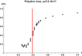
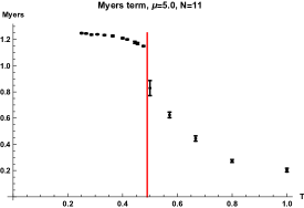
Figure 1: The Polyakov loop (top) and the Myers term (bottom) for $\mu=5.0$, $N=11$. The transition temperatures of the Myers term and of the Polyakov loop are around $T_{c1}=0.490$ and $T_{c2}=0.390$, respectively.

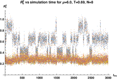
Figure 2: The Polyakov loop (top left), the Myers term (top right) and $R^{2}_{ii}$ at $T_{c1}=0.690$ (bottom) for $\mu=6.0$, $N=8$. The transition temperatures of the Myers term and of the Polyakov loop are around $T_{c1}=0.690$ and $T_{c2}=0.465$, respectively. The upper bluish points in the plot for $R^{2}_{ii}$ correspond to the $SO(3)$ matrices and the lower reddish points correspond to the $SO(6)$ matrices.

The left graphs in Fig. 1 and 2 show a transition in the Polyakov loop. Since the Polyakov loop is an order parameter for the confinement/deconfinement transition, this transition involves a change of the eigenvalue distribution of the gauge field from the uniform one to a non-uniform one. At this point, it is not clear yet whether there exists only one transition or more transitions in the transition region in the Polyakov loop; however, at least a gapped distribution is observed at high temperatures and an ungapped one at temperatures slightly lower than the transition temperature marked as the red vertical line for the Polyakov loop. Note that the transition observed in the numerical simulation is merely effective because the true phase transition exists only in the large-$N$ limit.

On the other hand, the right graphs in Fig. 1 and 2 show another transition, detected by the Myers term, which we call the Myers transition in the paper. One can see the two transition temperatures are distinct by comparing the positions of two red vertical lines in the right and left graphs. In fact, what the Myers term captures is completely different. The bottom graph in Fig. 2 is a Monte-Carlo history of $R^{2}_{ii}$ at the transition temperature $T_{c1}=0.690$ marked as the red vertical line in the top right graph. It shows large fluctuations between three different levels for the $SO(3)$ matrices, $X^{a}$. Each level corresponds to one or more vacua of the BMN matrix model; hence the fluctuations in the plot are transitions between vacua. Since these levels are what the Myers term measures, the transition in the Polyakov loop is essentially different from the Myers transition.

As the temperature decreases, the system undergoes the Myers transition before the confinement/deconfinement transition. At higher temperatures, the system is in a phase where thermal fluctuations are around the trivial vacuum. With decreasing temperature, the system enters the Myers transition region and then hops among different vacua, seen in Fig. 2. After the transition, it stays at a certain vacuum with non-zero $SU(2)$ spins. Let us call it a fuzzy-sphere phase. Spins of a vacuum in the final phase vary by value of $\mu$; the smaller the value of $\mu$, the larger a typical value of spins.

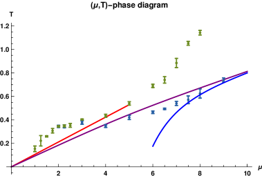
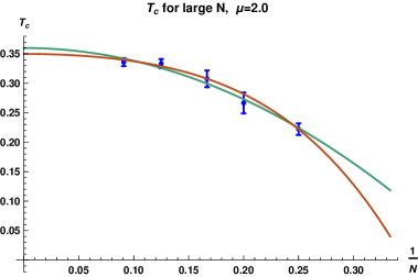
Figure 3: The observed phase diagram in the $\mu$–$T$ plane for $N=8$ and $\Lambda=24$ (left) and large-$N$ extrapolation of the transition temperature of the Myers transition at $\mu=2.0$ (right). On the left figure, the green and dark blue points respectively represent the Myers transition and the Polyakov-loop transition. The blue curve is the large-$\mu$ expansion of the critical temperature to three-loop order, the red line is the gravity prediction, and the purple curve is the Padé approximant obtained from the large-$\mu$ expansion. On the right figure, observed data are of $N=4,5,6,8$ and $11$. The green curve is a quadratic extrapolation: $0.36-2.17/N^{2}$ while the red curve is a quartic one: $0.35-1.09/N^{2}-15.26/N^{4}$.

The left graph in Fig. 3 is the resultant phase diagram for $N=8$ with $\Lambda=24$. Though not presented here, we confirmed the perfect agreement with the large-$\mu$ expansion of the critical temperature [48, 49], at large $\mu$ such as $\mu=14,18$. Surprisingly, the two transitions appear to merge around $\mu=3$. Although it is difficult to determine the transition temperature in the Polyakov loop at $\mu\lesssim 2$, we can estimate it approximately, and it seems the two transition temperatures coincide. Thus we naturally assume the critical temperature of the confinement/deconfinement transition is equivalent to that of the Myers transition in this region. Then the transition temperature seems to approach the theoretical prediction from the gravity side.

Although the matrix size is fixed to $N=8$ in the phase diagram, it is seen that the finite-$N$ effect is negligible at $\mu=2.0$, from the large-$N$ extrapolation of the transition temperature, shown in the right graph of Fig. 3.

4 Summary and Discussion

As to the emergent geometries embedded in the BMN matrix model, we have seen that both the geometries in the supergravity picture and those in the brane picture are reproduced by the eigenvalue distribution of the BPS operator $\phi$.

In the supergravity picture, the supergravity solutions are described by a single function $V(r,z)$. Through the gauge/gravity dictionary (10), this function can be constructed by the eigenvalue density of $\phi$ on the gauge-theory side.

In the brane picture, the geometry of M2-branes or M5-branes is a two-sphere or a five-sphere, respectively. Its radius is determined by the light-cone Hamiltonian of M-branes. Then, by the symmetric uplift of the eigenvalue distribution of $\phi$, a sphere wrapped by M2-branes or M5-branes is reproduced with the expected radius. For M2-branes, this is understood as the Myers effect [50] as well.

It provides a unified view that a single BPS operator $\phi$ describes both the supergravity solution and the brane geometry. However, it still remains obscure how exactly this equivalence of the matrix model to the brane picture is related with the equivalence to the supergravity picture in the gauge/gravity duality. If the equivalence among these three pictures is established in the BMN-model case, one can expect deeper understanding of the gauge/gravity conjecture in general.

Another important aspect is relationship to the non-commutative geometry. In the case of the 2-brane, the emergent $S^{2}$ geometry is constructed by a fuzzy 2-sphere as a result of the Myers effect. Meanwhile, for the 5-brane, a concrete construction of $S^{5}$ by a set of matrices in the BMN model as a non-commutative sphere has not been obtained yet. The difficulty stems from the fact that the $S^{5}$ is realised thanks to the quantum effect while the realisation of the $S^{2}$ can be seen even at the classical level. Although the BPS operator $\phi$ overcomes the difficulty of the quantum effect thanks to the supersymmetry, it fails to offer a matrix form of the geometry at this point.

The numerical results showed an intriguing insight into a dynamical aspect of the emergent geometries, namely, a geometrical interpretation given by the Myers transition. Since each vacuum corresponds to a supergravity solution, the Myers transition represents a transition between supergravity solutions. At high temperatures, the system is around the trivial vacuum, the spin-0 representation. Since this is in the deconfinement phase, the corresponding gravity solution is the one in Ref. [40]. As the temperature decreases, the system hits the phase boundary of the Myers transition so that the system is transitioned to a fuzzy-sphere vacuum, which corresponds to another supergravity solution. Until it undergoes another phase transition—the confinement/deconfinement transition—the gravity solution corresponding to the phase would be a Lin-Maldacena-like black-hole geometry with a non-trivial horizon topology, which has not been discovered yet. Then as the temperature decreases further, the corresponding gravity solution should become a thermal Lin-Maldacena geometry without a horizon. However, it should require more to understand the exact meaning of these interpretations. In order for the classical supergravity picture or the brane picture to be valid, one needs to take a proper large-$N$ limit; $N\approx 10$ may be insufficient to see geometries. In addition, it can be obscure whether the high-temperature phase has a good geometrical meaning at intermediate $\mu$ because at high temperatures it is described by the perturbative matrix model rather than by the gravity solution.

Another remark on the emergent geometries observed in the numerical simulation is the Myers transition at small $\mu$ looks like a transition to a vacuum corresponding to 5-branes. The observation was the Myers term in the fuzzy-sphere phase looked independent of $N$ [1]. In the simple setup (4), the Myers term (19) behaves as $\sim\mu^{3}(N_{5}^{2}-1)$. Thus it is likely that a typical dimension of irreducible representations does not grow as $N$ increases while a typical multiplicity grows linearly, which suggests the phase of such a vacuum corresponds to 5-branes [41].

The two observed phase transitions give different transition temperatures in the intermediate region of $\mu$. The numerical simulation revealed that these two transitions do not merge at $3\lesssim\mu\lesssim 6$ for $N=8$ on the lattice while it appears they merge below $\mu\approx 3$. There is no theoretical explanation of this behaviour thus far.

We conclude the simulation result is consistent with the gravity prediction obtained in Ref. [40]. The numerical result in Fig. 3 shows qualitative agreement with the expected critical temperature of the confinement/deconfinement transition (17). Strictly speaking, we need to keep the system around the trivial vacuum below the transition temperature of the Myers transition for more rigorous agreement because the obtained gravity prediction corresponds to the trivial vacuum. Since all vacua are stable at zero temperature, this seems possible in practice if one manipulates a simulation so as not to let the system undergo the Myers transition. However, as the confinement/deconfinement transition seems to merge with the Myers transition at small $\mu$, the obtained transition temperature should be a reasonable estimate of the critical temperature for the trivial vacuum. Moreover, it was found that the trivial vacuum gives a higher transition temperature in the Polyakov loop than fuzzy-sphere vacua [1]. This observation is also consistent with the prediction that (17) is an upper bound.

There are much more to study numerically in the low-temperature region. Since the gravity side at zero temperature is described by droplet solutions, we expect a richer structure at lower temperatures, which should reflect geometrical information. It would be a real challenge to reveal the complete phase structure due to more computational cost. This is because, at lower temperatures, the lattice effect becomes larger and, more importantly, one needs to carefully deal with contributions from all vacua as they are expected to be (meta-)stable. Further numerical studies in this region will enhance our understanding of dynamics of emergent geometries.

There are other intriguing directions related with the BMN-model simulation.

One example is the bosonic BMN matrix model, the action of which has only the bosonic part of the full BMN matrix model. In Ref. [51], we found that there are two transitions at finite $N$ in the eigenvalue distribution of the gauge field—a uniform-to-non-uniform transition and an ungapped-to-gapped transition—but also that these two converge to a single first-order transition in the large-$N$ limit. This may suggest the transition observed in the Polyakov loop in the full BMN matrix model is also a single first-order transition. The behaviour of the Polyakov loop is further studied in terms of counting states in an upcoming paper (see Ref. [52]).

Another direction is to study matrix models for longitudinal M5-branes. While M5-branes appearing in the BMN matrix model are transverse to the M-theory direction, those in the Berkooz-Douglas (BD) matrix model [53], which is the BFSS matrix model probing D4-branes, are longitudinal to the direction. There have been numerical results of the BD model, and they showed the agreement in the gauge/gravity duality [54, 55]. More interestingly, there is proposed a BMN-like mass-deformed version of the BD matrix model [56], which is supposed to describe M-theory on the plane-wave background probing longitudinal M5-branes.

- [1] Y. Asano, V. G. Filev, S. Kováčik and D. O’Connor, The non-perturbative phase diagram of the BMN matrix model, JHEP 1807 (2018) 152.
- [2] B. de Wit, J. Hoppe and H. Nicolai, On the Quantum Mechanics of Supermembranes, Nucl. Phys. B 305, 545 (1988).
- [3] T. Banks, W. Fischler, S. H. Shenker and L. Susskind, M theory as a matrix model: A Conjecture, Phys. Rev. D 55, 5112 (1997).
- [4] N. Ishibashi, H. Kawai, Y. Kitazawa and A. Tsuchiya, A Large N reduced model as superstring, Nucl. Phys. B 498 (1997) 467.
- [5] D. E. Berenstein, J. M. Maldacena and H. S. Nastase, Strings in flat space and pp waves from N=4 superYang-Mills, JHEP 0204, 013 (2002).
- [6] K. Dasgupta, M. M. Sheikh-Jabbari and M. Van Raamsdonk, Protected multiplets of M theory on a plane wave, JHEP 0209, 021 (2002).
- [7] G. Ishiki, S. Shimasaki, Y. Takayama and A. Tsuchiya, Embedding of theories with SU(2—4) symmetry into the plane wave matrix model, JHEP 0611 (2006) 089.
- [8] T. Ishii, G. Ishiki, S. Shimasaki and A. Tsuchiya, N=4 Super Yang-Mills from the Plane Wave Matrix Model, Phys. Rev. D 78 (2008) 106001.
- [9] Y. Kitazawa and K. Matsumoto, N=4 Supersymmetric Yang-Mills on S**3 in Plane Wave Matrix Model at Finite Temperature, Phys. Rev. D 79, 065003 (2009).
- [10] G. Ishiki, S. Shimasaki and A. Tsuchiya, Perturbative tests for a large-N reduced model of super Yang-Mills theory, JHEP 1111, 036 (2011).
- [11] Y. Asano, G. Ishiki, T. Okada and S. Shimasaki, Exact results for perturbative partition functions of theories with SU(2—4) symmetry, JHEP 1302 (2013) 148.
- [12] G. Ishiki, S. W. Kim, J. Nishimura and A. Tsuchiya, Deconfinement phase transition in N=4 super Yang-Mills theory on R x S**3 from supersymmetric matrix quantum mechanics, Phys. Rev. Lett. 102, 111601 (2009).
- [13] G. Ishiki, S. W. Kim, J. Nishimura and A. Tsuchiya, Testing a novel large-N reduction for N=4 super Yang-Mills theory on R x S**3, JHEP 0909 (2009) 029.
- [14] H. Lin and J. M. Maldacena, Fivebranes from gauge theory, Phys. Rev. D 74, 084014 (2006).
- [15] H. Lin, O. Lunin and J. M. Maldacena, Bubbling AdS space and 1/2 BPS geometries, JHEP 0410, 025 (2004).
- [16] V. Pestun, Localization of gauge theory on a four-sphere and supersymmetric Wilson loops, Commun. Math. Phys. 313, 71 (2012).
- [17] Y. Asano, G. Ishiki, T. Okada and S. Shimasaki, Emergent bubbling geometries in the plane wave matrix model, JHEP 1405, 075 (2014).
- [18] Y. Asano, G. Ishiki and S. Shimasaki, Emergent bubbling geometries in gauge theories with SU(2—4) symmetry, JHEP 1409, 137 (2014).
- [19] Y. Asano, G. Ishiki, S. Shimasaki and S. Terashima, Spherical transverse M5-branes in matrix theory, Phys. Rev. D 96, no. 12, 126003 (2017).
- [20] Y. Asano, G. Ishiki, S. Shimasaki and S. Terashima, Spherical transverse M5-branes from the plane wave matrix model, JHEP 1802 (2018) 076.
- [21] D. Berenstein, A Toy model for the AdS / CFT correspondence, JHEP 0407, 018 (2004).
- [22] Y. Takayama and A. Tsuchiya, Complex matrix model and fermion phase space for bubbling AdS geometries, JHEP 0510, 004 (2005).
- [23] D. Berenstein, Large N BPS states and emergent quantum gravity, JHEP 0601, 125 (2006).
- [24] D. Berenstein, D. H. Correa and S. E. Vazquez, All loop BMN state energies from matrices, JHEP 0602, 048 (2006).
- [25] M. Hanada, J. Nishimura and S. Takeuchi, Non-lattice simulation for supersymmetric gauge theories in one dimension, Phys. Rev. Lett. 99 (2007), 161602.
- [26] S. Catterall and T. Wiseman, Towards lattice simulation of the gauge theory duals to black holes and hot strings, JHEP 12 (2007), 104.
- [27] K. N. Anagnostopoulos, M. Hanada, J. Nishimura and S. Takeuchi, Monte Carlo studies of supersymmetric matrix quantum mechanics with sixteen supercharges at finite temperature, Phys. Rev. Lett. 100 (2008), 021601.
- [28] S. Catterall and T. Wiseman, Black hole thermodynamics from simulations of lattice Yang-Mills theory, Phys. Rev. D 78 (2008), 041502.
- [29] M. Hanada, Y. Hyakutake, J. Nishimura and S. Takeuchi, Higher derivative corrections to black hole thermodynamics from supersymmetric matrix quantum mechanics, Phys. Rev. Lett. 102 (2009), 191602.
- [30] M. Hanada, Y. Hyakutake, G. Ishiki and J. Nishimura, Holographic description of quantum black hole on a computer, Science 344 (2014), 882-885.
- [31] D. Kadoh and S. Kamata, Gauge/gravity duality and lattice simulations of one dimensional SYM with sixteen supercharges, arXiv:1503.08499 [hep-lat].
- [32] V. G. Filev and D. O’Connor, The BFSS model on the lattice, JHEP 1605 (2016) 167.
- [33] E. Berkowitz, E. Rinaldi, M. Hanada, G. Ishiki, S. Shimasaki and P. Vranas, Precision lattice test of the gauge/gravity duality at large-, Phys. Rev. D 94 (2016) no.9, 094501.
- [34] M. Hanada, A. Miwa, J. Nishimura and S. Takeuchi, Schwarzschild radius from Monte Carlo calculation of the Wilson loop in supersymmetric matrix quantum mechanics, Phys. Rev. Lett. 102 (2009), 181602.
- [35] M. Hanada, J. Nishimura, Y. Sekino and T. Yoneya, Monte Carlo studies of Matrix theory correlation functions, Phys. Rev. Lett. 104 (2010), 151601.
- [36] M. Hanada, J. Nishimura, Y. Sekino and T. Yoneya, Direct test of the gauge-gravity correspondence for Matrix theory correlation functions, JHEP 12 (2011), 020.
- [37] S. Catterall and G. van Anders, First Results from Lattice Simulation of the PWMM, JHEP 1009 (2010) 088.
- [38] M. Honda, G. Ishiki, S. W. Kim, J. Nishimura and A. Tsuchiya, Direct test of the AdS/CFT correspondence by Monte Carlo studies of N=4 super Yang-Mills theory, JHEP 1311 (2013) 200.
- [39] D. Schaich, R. G. Jha and A. Joseph, Thermal phase structure of a supersymmetric matrix model, \posPoS(LATTICE2019)069 (2020).
- [40] M. S. Costa, L. Greenspan, J. Penedones and J. Santos, Thermodynamics of the BMN matrix model at strong coupling, JHEP 1503 (2015) 069.
- [41] J. M. Maldacena, M. M. Sheikh-Jabbari and M. Van Raamsdonk, Transverse five-branes in matrix theory, JHEP 0301, 038 (2003).
- [42] H. Ling, A. R. Mohazab, H. Shieh, G. van Anders and M. Van Raamsdonk, Little string theory from a double-scaled matrix model, JHEP 10 (2006), 018.
- [43] V. G. Filev and D. O’Connor, Multi-matrix models at general coupling, J. Phys. A 46 (2013) 475403.
- [44] V. G. Filev and D. O’Connor, On the Phase Structure of Commuting Matrix Models, JHEP 1408, 003 (2014).
- [45] I. R. Klebanov and A. A. Tseytlin, Entropy of near extremal black p-branes, Nucl. Phys. B 475 (1996), 164-178.
- [46] N. Itzhaki, J. M. Maldacena, J. Sonnenschein and S. Yankielowicz, Supergravity and the large N limit of theories with sixteen supercharges, Phys. Rev. D 58 (1998), 046004.
- [47] S. Hawking and D. N. Page, Thermodynamics of Black Holes in anti-De Sitter Space, Commun. Math. Phys. 87 (1983), 577.
- [48] M. Spradlin, M. Van Raamsdonk and A. Volovich, Two-loop partition function in the planar plane-wave matrix model, Phys. Lett. B 603 (2004), 239-248.
- [49] S. Hadizadeh, B. Ramadanovic, G. W. Semenoff and D. Young, Free energy and phase transition of the matrix model on a plane-wave, Phys. Rev. D 71 (2005), 065016.
- [50] R. C. Myers, Dielectric branes, JHEP 12 (1999), 022.
- [51] Y. Asano, S. Kováčik and D. O’Connor, The Confining Transition in the Bosonic BMN Matrix Model, arXiv:2001.03749 [hep-th].
- [52] S. Kováčik, D. O’Connor and Y. Asano, The nonperturbative phase diagram of the bosonic BMN matrix model, arXiv:2004.05820 [hep-th].
- [53] M. Berkooz and M. R. Douglas, Five-branes in M(atrix) theory, Phys. Lett. B 395 (1997), 196-202.
- [54] V. G. Filev and D. O’Connor, A Computer Test of Holographic Flavour Dynamics, JHEP 1605 (2016) 122.
- [55] Y. Asano, V. G. Filev, S. Kováčik and D. O’Connor, A computer test of holographic favour dynamics. Part II, JHEP 1803 (2018) 055.
- [56] N. Kim, K. Lee and P. Yi, Deformed matrix theories with N=8 and five-branes in the PP wave background, JHEP 11 (2002), 009.