Self-Supervised Attention Learning for Depth and Ego-motion Estimation

Abstract

We address the problem of depth and ego-motion estimation from image sequences. Recent advances in the domain propose to train a deep learning model for both tasks using image reconstruction in a self-supervised manner. We revise the assumptions and the limitations of the current approaches and propose two improvements to boost the performance of the depth and ego-motion estimation. We first use Lie group properties to enforce the geometric consistency between images in the sequence and their reconstructions. We then propose a mechanism to pay attention to image regions where the image reconstruction gets corrupted. We show how to integrate the attention mechanism in the form of attention gates in the pipeline and use attention coefficients as a mask. We evaluate the new architecture on the KITTI datasets and compare it to the previous techniques. We show that our approach improves the state-of-the-art results for ego-motion estimation and achieve comparable results for depth estimation.

I INTRODUCTION

The tasks of depth estimation and ego-motion are longstanding problems in computer vision; their successful solution is crucial for a wide variety of applications, such as autonomous driving, robot navigation, and visual localization, Augmented/Virtual Reality applications, etc.

In the last years, deep learning networks [6, 8, 17, 30] achieved results comparable with traditional geometric methods for depth estimation. They show competitive results in complex and ambiguous 3D areas, with CNNs serving as deep regressors and coupled with classical components, to get the best from the geometric and learning paradigms. For the ego-motion estimation, several works [16, 30] have achieved a level of performance comparable to the traditional techniques based on the SLAM algorithm [12, 19, 20]. Early methods for depth and ego-motion (DEM) are based on supervised learning; they require large annotated datasets and calibrated setups. Trained and tested on publicly available benchmark datasets, these techniques show a limited capacity to generalize beyond the data they are trained on.

Moreover, data annotation is often slow and costly. The annotations also suffer from the structural artifacts, particularly in the presence of reflective, transparent, dark surfaces or non-reflective sensors that output infinity values. All these challenges strongly motivated the shift to the unsupervised learning of depth and ego-motion, in particular from monocular (single-camera) videos.

To enable the DEM estimation without annotations, the major idea is to process both tasks jointly [30]. In the self-supervised setting, an assumption is made about spatial consistency and temporal coherence between consecutive frames in a sequence. The only external data needed is the camera intrinsics. Recent progress in the domain [18, 28, 26, 3] allows us to use monocular unlabeled videos to provide self-supervision signals to a learning component. The 3D geometry estimation includes per-pixel depth estimation from a single image and 6DoF relative pose estimation between neighbor images.

Self-supervised learning greatly boosted DEM estimation performance. There however remains a gap with the related supervised methods. The underlying assumption of the static world is often violated in real scenes and the geometric image reconstruction gets corrupted by unidentified moving objects, occlusions, reflection effects, etc.

Multiple improvements have been recently proposed to address these issues [1, 3, 18, 26, 27]. They are often based on adding more components to the architecture such as flow nets [27], semantic segmentation [18], adversarial networks [1], and multiple masks [26]. These approaches lead however to an important growth of model parameters, making the architecture and training procedure more complex.

In this paper, we propose an alternative and effective solution to the problem-based on the attention mechanism [15]. Initially proposed for natural language processing tasks [4], the attention and its variants have been successfully extended to computer vision tasks, including image classification [25], semantic segmentation [13, 21], image captioning  [29], and depth estimation  [28]. Inspired by these successes, we propose to include the attention mechanism in self-supervised learning for DEM estimation. We show that so-called attention gates can be integrated into the baseline architecture and trained from scratch to automatically learn to focus on corrupted regions without additional supervision.

The attention gates do not require a large number of model parameters and introduce a minimal computational overhead. In return, the proposed mechanism improves model sensitivity and accuracy for dense depth and ego-motion estimation.

The attention gates are integrated into the depth estimation network. Consequently, the depth network can predict both the depth estimation and attention coefficients which are then used to weigh the difference between the true and reconstructed pixels when minimizing the objective function.

We evaluate the proposed architecture on the KITTI datasets and compare it to the state of the art techniques. We show that our approach improves the state-of-the-art results for ego-motion estimation and achieve comparable results for depth estimation.

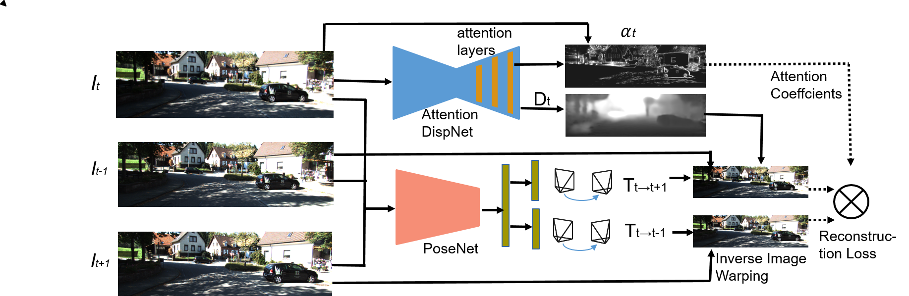
Figure 1: Attention-based DEM architecture.

II RELATED WORK

Eigen at al. [7] was first to directly regress a CNN over pixel values and to use multi-scale features for monocular depth estimation. They used the global (coarse-scale) and local (fine-scale) networks to accomplish the tasks of global depth prediction and local refinements.

Garg et al. [8] proposed to use a calibrated stereo camera pair setup where the depth is produced as an intermediate output and the supervision comes as a reconstruction of one image from another in a stereo pair. Images on the stereo rig have a fixed and known transformation, and the depth can be learned from this functional relationship.

An important step forward was developed in Godard et al. [10] where the depth estimation problem was reformulated in a new way. Godard et al. employ binocular stereo pairs of a view in training but, during inference time, one view is only used to estimate the depth. By exploiting epipolar geometry constraints, they generate disparity images by training their network with an image reconstruction loss. The model does not require any labeled depth data and learns to predict pixel-level correspondences between pairs of rectified stereo images.

Mahjourian et al. [18] made another step by using camera ego-motion and 3D geometric constraints. Zhou et al. [30] proposed a novel approach for unsupervised learning of depth and ego-motion from monocular video only. An additional module to learn the motion of objects was introduced in [24]; however, their architecture recommends optional supervision by ground-truth depth or optical flow to improve performance.

The static world assumption doe not hold in real scenes, because of unidentified moving objects, occlusions, photo-effects, etc. that violate the underlying assumption and corrupt the geometric image reconstruction. The recent works address these limitations and propose several improvements, varying from new objective functions, additional modules and pixel masking to new learning schemes.

Almalioglu at al. [1] proposed a framework that predicts pose camera motion and a monocular depth map of the scene using deep convolutional Generative Adversarial Networks (GANs). An additional adversarial module helps learn more accurate models and make reconstructed images indistinguishable from the real images.

Wang et al. [26] coped with errors in realistic scenes due to reflective surfaces and occlusions. They combined the geometric and photometric losses by introducing the matching loss constrained by epipolar geometry and designed multiple masks to solve image pixel mismatch caused by the movement of the camera.

Another solution was proposed in UnDEMoN architecture [2]. The authors changed the objective function and tried to minimize spatial and temporal reconstruction losses simultaneously. These losses are defined using a bi-linear sampling kernel and penalized using the Charbonnier penalty function.

Most recently, Bian et al.[3] analyzed violations of the underlying static assumption in geometric image reconstruction and concluded that, due to lack of proper constraints, networks output scale-inconsistent results over different samples. To remedy the problem, the authors proposed a geometry consistency loss for scale-consistent predictions and a mask for handling moving objects and occlusions. Since our approach does not leverage additional modules nor multi-task learning, our attention-based framework is much simpler and more efficient.

III Baseline architecture and extensions

Similar to the recent methods [18, 26, 30], our baseline architecture includes depth estimation and pose estimation modules. The depth module is an encoder-decoder network (DispNet); it takes a target image and outputs depth values $\hat{D}_{t}(p)$ for every pixel $p$ in the image. The pose module (PoseNet) take as input the concatenation of the target image $I_{t}$ and two neighbors (source) images $I_{s}$, $s\in\{t-1,t+1\}$. It outputs transformation matrices $\hat{T}_{t\rightarrow s}$, representing the six degrees of freedom (6DoF) relative pose between the images.

III-1 Image reconstruction

Self-supervised learning is proceeded by image reconstruction using the inverse warping technique [10]. This technique is differentiable, therefore it allows us to back-propagate the gradients during training. It tries to reconstruct the target image $I_{t}$ through sampling pixels from the source images $I_{s}$ based on the estimated depth map $\hat{D}_{t}$ and the relative pose transformation matrices $\hat{T}_{t\rightarrow s}$, $s\in\{t-1,t+1\}$. The sampling is done by projecting the homogeneous coordinates of the target pixel $p_{t}$ onto the source view $p_{s}$. Given the camera intrinsics $K$, the estimated depth of the pixel $\hat{D}_{t}(p)$ and transformation matrix $\hat{T}_{t\rightarrow s}$, the projection is done by the following equation.

$$p_{s}\sim K\hat{T}_{t\rightarrow s}\hat{D}_{t}(p_{t})K^{-1}p_{t}.$$ (1)

For non-discrete values of a projected pixel position, the differentiable bi-linear sampling interpolation [14] is used to find the intensity value at a given position. The mean intensity value in the reconstructed image $\hat{I_{s}}$ is interpolated using 4-pixel neighbors of $p_{s}$ (top-right, top-left, bottom-right, bottom-left), as follows

$$\hat{I}_{s}(p_{t})=I_{s}(p_{s})=\sum_{i\in\{t,b\},j\in\{l,r\}}w^{ij}I_{s}(p_{s}^{ij}),$$ (2)

Where $\hat{I}_{s}(p_{t})$ is the intensity value of $p_{t}$ in the reconstructed image $\hat{I_{s}}$. The weight is linearly proportional to the spatial proximity between $p_{s}$ and the neighbor $p_{s}^{ij}$; the four weights $w^{ij}$ sum to 1.

III-2 Photometric Loss

Under the static world assumption, many existing methods apply the photometric loss [1, 23] defined as $L_{1}$ loss objective function: $\mathcal{L}_{p}=\sum_{s}\sum_{p}|I_{t}(p)-\hat{I}_{s}(p)|$.

Any violation of the static world assumption in the real scenes affects drastically the reconstruction. To overcome this limitation, one solution is to use the SSID loss [18, 26, 23]. A more advanced solution [30] is to introduce an explainability mask to indicate the importance of a pixel in the warped images. If the pixel contributes to a corrupted synthesis the explainability value of the pixel will be negligible.

The explainability values are produced by a dedicated module (ExpNet) in [30]; it shares the encoder with the PoseNet and branches off in the decoding part. The three networks(DispNet, PoseNet and ExpNet) are trained simultaneously. The ExpNet decoder generates a per-pixel mask $\hat{E}_{k}(p)$. Similar to PoseNet, the explainability map $\hat{E}_{k}$ is generated for both source images. Per-pixel explainability values are embedded in the photometric loss:

$$\mathcal{L}_{p}=\frac{1}{|V|}\sum_{p}\hat{E}_{k}(p)|I_{t}(p)-\hat{I}_{s}(p)|~{}.$$ (3)

where $|V|$ is the number of pixels in the image. To avoid a trivial solution in (3) with $\hat{E}_{k}(p)$ equals to zero, a constraint is added on the values of $\hat{E}_{k}(p)$. This constraint is implemented as a regularization loss $\mathcal{L}_{reg}(\hat{E}_{k})$, defined as a cross entropy loss between the mask value and a constant 1.

III-3 Depth smoothness

We follow [23] in including a smoothness term to resolve the gradient-locality issue and remove discontinuity of the learned depth in low-texture regions. We use the edge-aware depth smoothness loss which uses image gradient to weigh the depth gradient:

$$L_{smo}=\sum_{p}|\nabla D(p)|^{T}\cdot e^{-|\nabla I(p)|},$$ (4)

where $p$ is the pixel on the depth map $D$ and image $I$, $\nabla$ denotes the 2D differential operator, and $|\cdot|$ is the element-wise absolute value. We apply the smoothness loss on three additional intermediate layers from DispNet.

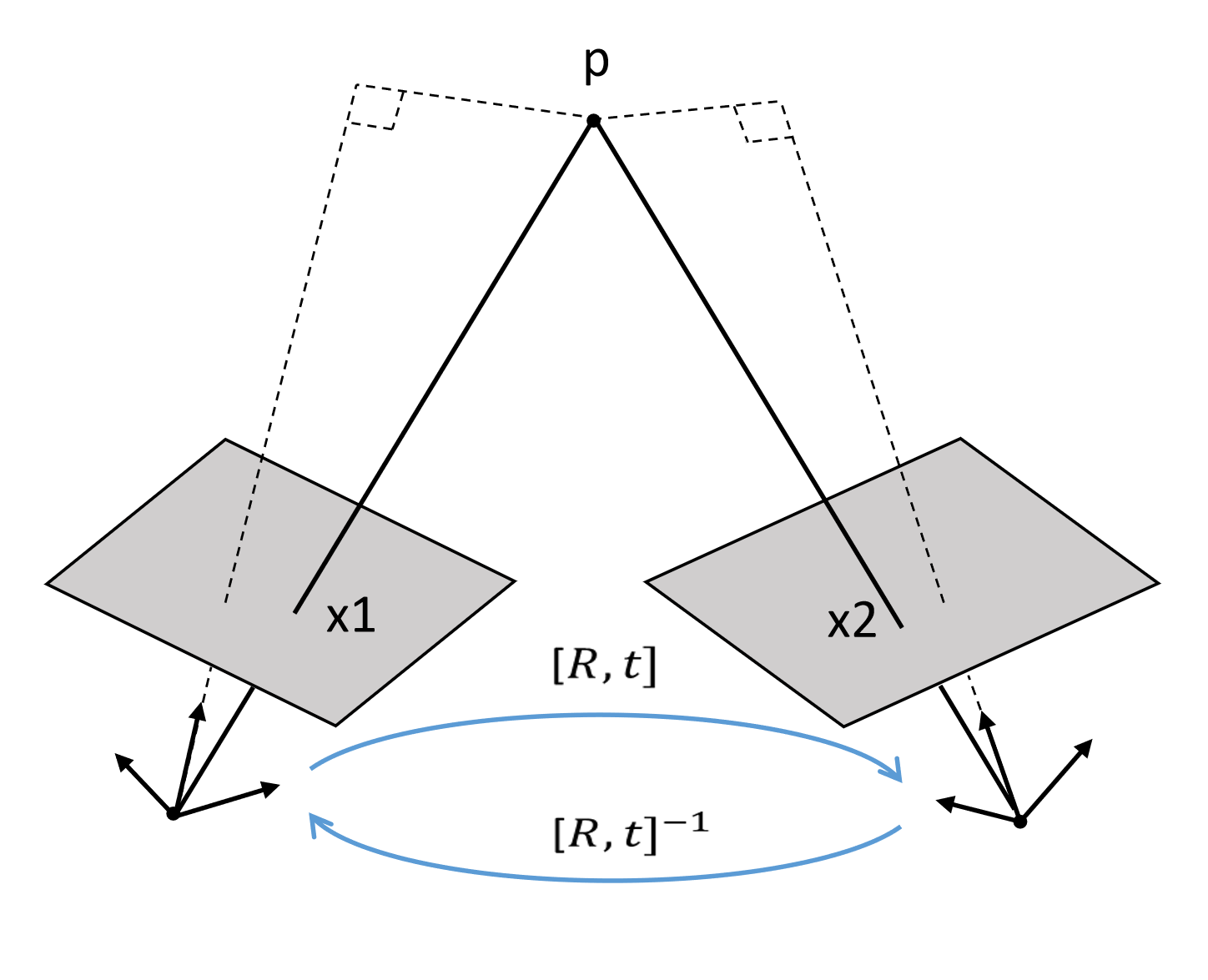
Figure 2: Relative transformation between two different views for the same camera.

III-A Backward-Forward Consistency

The baseline architecture presented in the previous section integrates all components that proved their efficiency in the state of the art methods. Now we propose the first extension of our architecture and consider reinforcing the geometric consistency by using the Lie group property [5].

Indeed, the set of 3D space transformations $T$ form a Lie group $\mathbb{SE}(3)$; it is represented by linear transformations on homogeneous vectors, $T=[{\bf R,t}]\in\mathbb{SE}(3)$, with the rotation component $\mathbf{R}\in\mathbb{SO}(3),$ and translation component $\>\mathbf{t}\in\mathbb{R}^{3}$. For every transformation $T\in\mathbb{SE}(3)$, there is an inverse transformation $T^{-1}\in\mathbb{SE}(3)$, such that $TT^{-1}=I$ (see Figure 2).

The PoseNet estimates relative pose transformations from a given target to the source frames. Therefore, for every pair of neighbour frames $(t-1,t)$ or $(t,t+1)$, we obtain the forward transformation $\hat{T}_{t-1\rightarrow t}$ as well as the backward one $\hat{T}_{t\rightarrow t-1}$. We can get the two transformations by changing the order of the concatenation images.

In a general case, for every pair of transformations $\hat{T}_{t\rightarrow s}$ and $\hat{T}_{s\rightarrow t}$, we impose an additional forward-backward geometric constraint; it requires the product of forward and backward transformations to be as close as possible to the identity matrix $I_{4x4}\in\mathbb{SE}(3)$. The corresponding loss is defined over for all pairs of relative pose transformations:

$$\mathcal{L}_{bf}=\sum_{s}\sum_{t}|\hat{T}_{s\rightarrow t}\hat{T}_{t\rightarrow s}-I_{4x4}|~{}.$$ (5)

The total training loss is given by

$$\mathcal{L}_{total}=\mathcal{L}_{p}+\lambda_{smo}\mathcal{L}_{smo}+\lambda_{reg}\mathcal{L}_{reg}+\lambda_{bf}\mathcal{L}_{bf},$$ (6)

where $\lambda_{smo}$, $\lambda_{reg}$, $\lambda_{bf}$ are hyper-parameters. In the experiments, $\lambda_{smo}=0.1$, $\lambda_{reg}=0.1$ and $\lambda_{bf}=0.1$, as showing the most stable results.

III-B Self-attention gates

Our second extension of the baseline architecture addresses the attention mechanism and lets the network know where to look as it is performing the task of DEM estimation.

Unlike integrating attention in Conditional Random Fields [28], our proposal is inspired by the recent works in semantic segmentation [15] in particular in medical imaging [21, 22]. We treat attention in-depth estimation similarly to semantic segmentation. If we consider that each instance (a group of pixels) belongs to a certain semantic label (e.g. pedestrian), then the same group of pixels will have close and discontinuous depth values. Hence, we pay attention to any violation of this principle as a potential source of corrupted image reconstruction.

We propose to integrate the attention mechanism in the depth module (DispNet). As shown in Figure 3, the encoder does not change, while the decoder layers are interleaved with the attention gates (AGs). The integration is done as follows.

Let ${\bf x}^{l}=\{{\bf x}_{i}^{l}\}^{n}_{i=1}$ be the activation map of a chosen layer $l\in\{1,\ldots,L\}$, where each ${\bf x}_{i}^{l}$ represents the pixel-wise feature vector of length $F_{l}$ (i.e. the number of channels). For each ${\bf x}_{i}^{l}$, AG computes coefficients $\alpha^{l}=\{\alpha_{i}^{l}\}^{n}_{i=1}$, $\alpha_{i}^{l}\in[0,1]$ to identify corrupted image regions, also, to prune feature responses that preserve only the activations relevant to the accurate depth estimation. The output of AG is ${\bf\hat{x}}^{l}=\{\alpha_{i}^{l}{\bf x}_{i}^{l}\}^{n}_{i=1}$ where each feature vector is scaled by the corresponding attention coefficient.

The attention coefficients $\alpha_{i}^{l}$ are computed as follows. In DispNet, the features on the coarse level identify the location of the target objects and model their relationship on a global scale. Let ${\bf g}\in\mathbb{R}^{F_{ge}}$ be such a global (coarser) feature vector providing information to AGs to disambiguate task-irrelevant feature content in ${\bf x}^{l}$. The idea is to consider each ${\bf x}^{l}$ and $\bf g$ jointly to attend the features at each scale $l$ that are most relevant to the objective being minimized.

The gating vector ${\bf g}$ contains contextual information to prune lower-level feature responses ${\bf x}_{i}^{l}$ as suggested in AGs for image classification [25]. And we prefer additive attention to the multiplicative one, as it has experimentally shown to achieve a higher accuracy [22]:

$$q^{l}_{att,i}$$=

=

(7)

where $\sigma_{1}(x)$ is an element-wise nonlinear function, in particular, we use $=\sigma_{1}(x)=\max(x,0)$ and $\sigma_{2}(x)$ is a sigmoid activation function. Each AG is characterized by a set of parameters $\Theta_{att}$ containing the linear transformations ${\bf W}_{x}\in\mathbb{R}^{F_{l}\times F_{int}}$, ${\bf W}_{g}\in\mathbb{R}^{F_{g}\times F_{int}}$, ${\bf W}_{a}\in\mathbb{R}^{F_{l}\times 1}$, and bias terms $b_{a}\in\mathbb{R}$, ${\bf b}_{x}$, ${\bf b}_{g}\in\mathbb{R}^{F_{int}}$. AG parameters can be trained with the standard back-propagation updates together with other DispNet parameters.

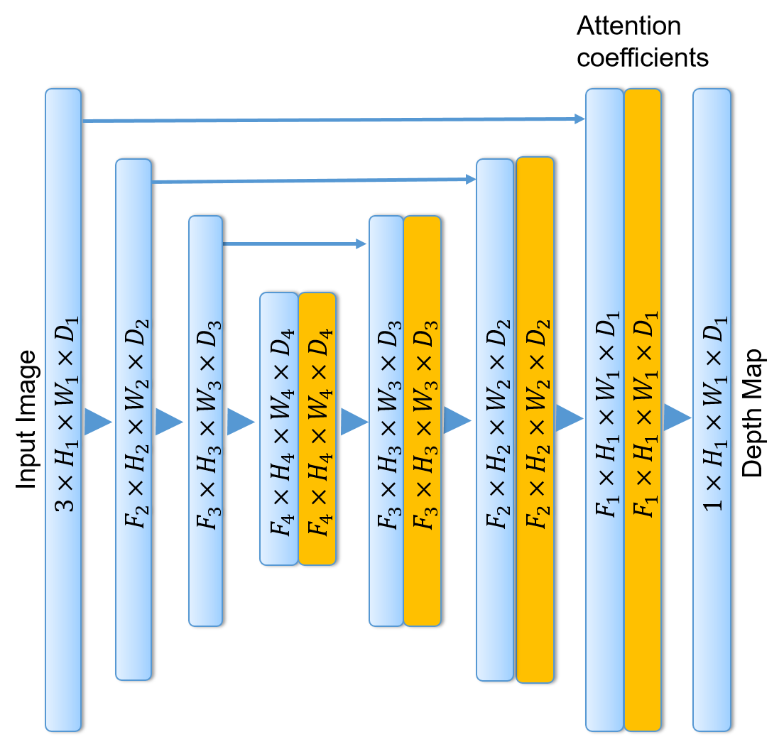
Figure 3: DispNet with the integrated attention gates (in orange). The input image is progressively filtered and downsampled by a factor of 2 at each scale $l$ in the encoding part of the network, $H_{i}=H_{1}/2^{i-1}$. Attention gates filter the features propagated through the skip connections by using the contextual information (gating) extracted in coarser scales.

With attention gates integrated into DispNet, we modify the photometric loss in (6) accordingly, with attention coefficient $\alpha$ for pixel $p$ used instead of explainability value $E(p)$. Figure 4 in Section IV visualizes the attention coefficients for three example images. It shows that the system pays less attention to moving objects, as well as to 2D edges and boundaries of regions with discontinuous depth values sensitive to the erroneous depth estimation.

IV EVALUATION RESULTS

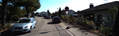
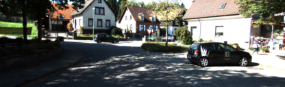
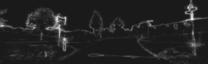
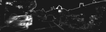
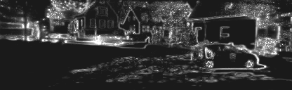
Figure 4: Original images from KITTI dataset (top) and the corresponding attention coefficient maps (bottom).

Method	Supervision	Error metric				Accuracy metric
		Abs Rel	Sq Rel	RMSE	RMSE log	$\delta<1.25$	$\delta<1.25^{2}$	$\delta<1.25^{3}$
Eigen et al. [7] Coarse	Depth	0.214	1.605	6.563	0.292	0.673	0.884	0.957
Eigen et al. [7] Fine	Depth	0.203	1.548	6.307	0.282	0.702	0.890	0.958
Liu et al. [17]	Pose	0.202	1.614	6.523	0.275	0.678	0.895	0.965
Godard et al. [10]	No	0.148	1.344	5.927	0.247	0.803	0.922	0.964
Zhou et al. [30] (w/o explainability)	No	0.221	2.226	7.527	0.294	0.676	0.885	0.954
Zhou et al. [30] (explainability)	No	0.208	1.768	6.856	0.283	0.678	0.885	0.957
Almalioglu et al. [1]	No	0.138	1.155	4.412	0.232	0.820	0.939	0.976
Shen et al. [23]	No	0.156	1.309	5.73	0.236	0.797	0.929	0.969
Bian et al. [3]	No	0.137	1.089	6.439	0.217	0.830	0.942	0.975
Ours (BF)	No	0.213	1.849	6.781	0.288	0.679	0.887	0.957
Ours (Attention)	No	0.171	1.281	5.981	0.252	0.755	0.921	0.968
Ours (BF+Attention)	No	0.162	1.126	5.284	0.221	0.823	0.935	0.971

TABLE I: Single-view depth results on the KITTI dataset [9] using the split of Eigen et al. [7] . Best and 2 runner-up results are shown in bold and italic, respectively.

In this section, we present the evaluation results of depth and ego-motion estimation, analyze them. We support our analysis with some visualizations, such as attention coefficients for masking pixels with likely corrupted image reconstruction.

IV-A Depth estimation

We evaluated the depth estimation on publicly available KITTI Raw dataset. It contains 42,382 rectified stereo pairs from 61 scenes. The Image size is 1242$\times$375. For the comparison with the previous works, we adopt the test split proposed by Eigen et al. [7]. The split consists of 697 images that cover a total of 29 scenes. The remaining 32 scenes (23,488 images) are used for training/validation split with 22,600/888 images respectively. We adopt the evaluation metrics already used in previous works [7, 11, 8]. They include the mean relative error (Abs Rel), the squared relative error (Sq Rel), the root mean squared error (RMSE), the mean $\log 10$ error (RMSE log), and the accuracy with threshold $t$ where $t\in[1.25,1.25^{2},1.25^{3}]$ (see [7] for more detail).

We test our architecture presented in Section III, in the baseline configuration, extended with Backward-Forward loss, attention gates, and both. Table I reports our depth evaluation results and compares them to the state of art methods.

As the table shows that our methods show state comparable, without using additional attention comparing to the baseline and it outperforms the supervised and most unsupervised techniques and shows performance comparable to the most recent methods [1, 3] which extend the baseline modules with additional modules and components.

Attention coefficients: Figure 4 visualizes the effect of attention coefficients as masks for down-weighting image regions that get corrupted It actually visualizes the inverse attention, where white color refers to the low attention coefficient $\alpha_{i}$, thus having a lower weight; the black color refer to high values.

We can see in the figure, that low attention coefficients point to pixels that have a high probability to be corrupted. First of all, it concerns image regions corresponding to the moving objects. In addition, the region with discontinuous depth values is considered as corrupted as well. This often includes region boundaries. Thin objects like street light and sign poles are also down-weighted because of the high probability of depth discontinuity and corrupted image reconstruction.

These results support the hypothesis for using attention coefficients as a mask. It represents an alternative to the explainability module in [30]. The region of interest is more likely the rigid object that the network will have more confidence to estimate their depth, it will be almost equal all over the object, like the segmentation problem. Also, the rigid objects are the most appropriate to estimate the change in position between frames, that is why it shut down the coefficient for the moving objects.

IV-B Pose estimation

We use the publicly available KITTI visual odometry dataset. The official split contains 11 driving sequences with ground truth poses obtained by GPS readings. We use sequence 09 and 10 to evaluate our approaches to align with previous SLAM-based works.

We follow the previous works in using the absolute trajectory error (ATE) as evaluation metric. It measures the difference between points of the ground truth and the predicted trajectory. Using timestamps to associate the ground truth poses with the corresponding predicted poses, we compute the difference between each pair of poses, and output the mean and standard deviation.

Table II reports the evaluation results of the Backward-Forward and attention modules, separately and jointly, and compare them to the previous works. Both extensions improve the baseline, the attention module performs well. When coupled with the BF, the attention boosts the performance of PoseNet training to have a consistent ego-motion estimation and outperforms all the state of the art methods [30, 18, 1, 23], which use additional models or pixel masks, thus increasing considerably the model size.

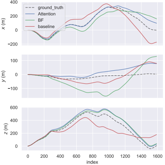
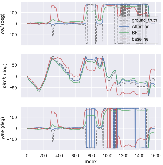
Figure 5: Sequence 09: Comparing the pose estimation to the ground truth, for each degree of freedom, including the translation $x,y,z$ (left) and rotation roll, pitch, yaw (right).

Figure 5 shows the 6-DoF estimated throughout the trip of the sequence 09. Our improvements are more robust compared to the baseline except in the altitude (y). The figure unveils another important issue. It demonstrates the oscillation of roll and yaw values and their discontinuity when put in $[-\pi,\pi]$ interval while orientation changes are continuous in the real world. A recent analysis of 3D and $n$-dimensional rotations [31] shows that discontinuous orientation representations make them difficult for neural networks to learn. Therefore, it might be a subject of deeper analysis and a need of replacing quaternions with an alternative, continuous representation.

Method	Seq. $09$	Seq. $10$
ORB-SLAM (full)	$0.014\pm 0.008$	$0.012\pm 0.011$
ORB-SLAM (short)	$0.064\pm 0.141$	$0.064\pm 0.130$
Zhou et al. [30] (baseline)	$0.016\pm 0.009$	$0.013\pm 0.009$
Mahjourian et al. [18]	$0.013\pm 0.010$	$0.012\pm 0.011$
Almalioglu et al. [1]	$0.009\pm 0.005$	$0.010\pm 0.0013$
Shen et al. [23]	$0.0089\pm 0.0054$	$0.0084\pm 0.0071$
Ours (BF)	$0.0101\pm 0.0065$	$0.0091\pm 0.0069$
Ours (Attention)	$0.0108\pm 0.0062$	$0.0082\pm 0.0063$
Ours (BF+Attention)	0.0087 $\pm$ 0.0054	0.0078 $\pm$ 0.0061

TABLE II: Absolute Trajectory Error (ATE) on the KITTI odometry split averaged over all frame snippets (lower is better).

IV-C Model size and the training time

Unlike the explainability, the attention gates do not require an additional networks, they are layers integrated into the existing depth network. Our architecture for DEM evaluation requires fewer parameters in the model and shows a faster training time than the state of the art methods. Indeed, adding the BF loss has a negligible impact on the training time with respect to the baseline. Adding attention gates increases the model size by 5-10% and training time by 10-25%. For the comparison, the training time of additional semantic segmentation [18] or GAN module [1] doubles the model size and requires 4-10 more time to train the models.

V CONCLUSIONS

We have presented two extensions of the baseline architecture for the depth and pose estimation tasks, all aimed to improve the performance in the self-supervised setting. Adding backward-forward consistency loss to the training process allowed to boost the performance. Our method follows one of the current trends forcing the learned models to respect the geometric principles but adding penalties for any consistency violation. This idea opens a possibility to explore and impose more geometric constraints on the learned models, this might further improve the accuracy. We have shown the effectiveness of attention gates integrated in the depth module of DEM estimation. It demonstrates that the attention principle can be expanded to the navigation tasks. The attention gates help identify corrupted image regions where the static world assumption is violated. Besides, the attention model can be explored as masking coefficients in multiple different ways, it represents a strong alternative to the explainability network in the baseline architecture.

References

- [1] Yasin Almalioglu, Muhamad Risqi U. Saputra, Pedro P. B. de Gusmao, Andrew Markham, and Niki Trigoni. GANVO: Unsupervised Deep Monocular Visual Odometry and Depth Estimation with Generative Adversarial Networks. In Proceedings of ICRA, 2019.
- [2] V. Madhu Babu, Kaushik Das, Anima Majumder, and Swagat Kumar. Undemon: Unsupervised deep network for depth and ego-motion estimation. In IEEE/RSJ International Conference on Intelligent Robots and Systems, IROS, pages 1082–1088, 2018.
- [3] Jiawang Bian, Zhichao Li, Naiyan Wang, Huangying Zhan, Chunhua Shen, Ming-Ming Cheng, and Ian D. Reid. Unsupervised scale-consistent depth and ego-motion learning from monocular video. In Proc. NIPS, pages 35–45, 2019.
- [4] Sneha Chaudhari, Gungor Polatkan, Rohan Ramanath, and Varun Mithal. An attentive survey of attention models. CoRR, abs/1904.02874, 2019.
- [5] José Luis Blanco Claraco. A tutorial on se(3) transformation parameterizations and on-manifold optimization. Technical report, 2019.
- [6] D. Eigen and R. Fergus. Predicting Depth, Surface Normals and Semantic Labels with a Common Multi-scale Convolutional Architecture. In Proc. IEEE International Conference on Computer Vision (ICCV), 2015.
- [7] David Eigen, Christian Puhrsch, and Rob Fergus. Depth Map Prediction from a Single Image using a Multi-Scale Deep Network. In Proc. NIPS, pages 2366–2374, 2014.
- [8] Ravi Garg, Vijay Kumar BG, Gustavo Carneiro, and Ian Reid. Unsupervised CNN for Single View Depth Estimation: Geometry to the Rescue. 3 2016.
- [9] Andreas Geiger, Philip Lenz, and Raquel Urtasun. Are we ready for Autonomous Driving? The KITTI Vision Benchmark Suite. Technical report.
- [10] Clément Godard, Oisin Mac Aodha, and Gabriel J. Brostow. Unsupervised Monocular Depth Estimation with Left-Right Consistency. In Proc. IEEE Conference on Computer Vision and Pattern Recognition, pages 6602–6611, 2017.
- [11] Clément Godard, Oisin Mac, Aodha Gabriel, and J Brostow. Unsupervised Monocular Depth Estimation with Left-Right Consistency. Technical report.
- [12] Cristopher Gómez, Matías Mattamala, Tim Resink, and Javier Ruiz-del Solar. Visual SLAM-based Localization and Navigation for Service Robots: The Pepper Case. 11 2018.
- [13] Qin Huang, Chunyang Xia, Chi-Hao Wu, Siyang Li, Ye Wang, Yuhang Song, and C.-C. Jay Kuo. Semantic segmentation with reverse attention. In Proc. BMVC, 2017.
- [14] Max Jaderberg, Karen Simonyan, Andrew Zisserman, and Koray Kavukcuoglu. Spatial Transformer Networks. 6 2015.
- [15] Saumya Jetley, Nicholas A. Lord, Namhoon Lee, and Philip H. S. Torr. Learn to pay attention. In Proc. International Conference on Learning Representations, ICLR, 2018.
- [16] Alex Kendall, Matthew Grimes, and Roberto Cipolla. PoseNet: A Convolutional Network for Real-Time 6-DOF Camera Relocalization. 5 2015.
- [17] Fayao Liu, Chunhua Shen, Guosheng Lin, and Ian Reid. Learning Depth from Single Monocular Images Using Deep Convolutional Neural Fields. IEEE Transactions on Pattern Analysis and Machine Intelligence, 2016.
- [18] Reza Mahjourian, Martin Wicke, and Anelia Angelova. Unsupervised Learning of Depth and Ego-Motion from Monocular Video Using 3d Geometric Constraints. In Proc. IEEE Conference on Computer Vision and Pattern Recognition, pages 5667–5675, 2018.
- [19] Raul Mur-Artal, J. M.M. Montiel, and Juan D. Tardos. ORB-SLAM: A Versatile and Accurate Monocular SLAM System. IEEE Transactions on Robotics, 31(5):1147–1163, 10 2015.
- [20] Raul Mur-Artal and Juan D. Tardos. ORB-SLAM2: An Open-Source SLAM System for Monocular, Stereo, and RGB-D Cameras. IEEE Transactions on Robotics, 33(5):1255–1262, 10 2017.
- [21] Ozan Oktay, Jo Schlemper, Loïc Le Folgoc, Matthew C. H. Lee, Mattias P. Heinrich, Kazunari Misawa, Kensaku Mori, Steven G. McDonagh, Nils Y. Hammerla, Bernhard Kainz, Ben Glocker, and Daniel Rueckert. Attention u-net: Learning where to look for the pancreas. arXiv:1804.03999, 2018.
- [22] Jo Schlemper, Ozan Oktay, Liang Chen, Jacqueline Matthew, Caroline Knight, Bernhard Kainz, Ben Glocker, and Daniel Rueckert. Attention-Gated Networks for Improving Ultrasound Scan Plane Detection. arXiv:1804.05338, 2018.
- [23] Tianwei Shen, Zixin Luo, Lei Zhou, Hanyu Deng, Runze Zhang, Tian Fang, and Long Quan. Beyond photometric loss for self-supervised ego-motion estimation. In Proc. International Conference on Robotics and Automation, ICRA, pages 6359–6365, 2019.
- [24] Sudheendra Vijayanarasimhan, Susanna Ricco, Cordelia Schmid, Rahul Sukthankar, and Katerina Fragkiadaki. SfM-Net: Learning of Structure and Motion from Video. arXiv:1704.07804, 2017.
- [25] Fei Wang, Mengqing Jiang, Chen Qian, Shuo Yang, Cheng Li, Honggang Zhang, Xiaogang Wang, and Xiaoou Tang. Residual attention network for image classification. In Proc. IEEE Conference on Computer Vision and Pattern Recognition, CVPR, pages 6450–6458, 2017.
- [26] G. Wang, H. Wang, Y. Liu, and W. Chen. Unsupervised learning of monocular depth and ego-motion using multiple masks. In Proc. International Conference on Robotics and Automation (ICRA), pages 4724–4730, May 2019.
- [27] Yang Wang, Zhenheng Yang, Peng Wang, Yi Yang, Chenxu Luo, and Wei Xu. Joint unsupervised learning of optical flow and depth by watching stereo videos. arXiv: 1810.03654, 2018.
- [28] Dan Xu, Wei Wang, Hao Tang, Hong Liu, Nicu Sebe, and Elisa Ricci. Structured Attention Guided Convolutional Neural Fields for Monocular Depth Estimation. arXiv:1803.11029, 2018.
- [29] Kelvin Xu, Jimmy Ba, Ryan Kiros, Kyunghyun Cho, Aaron C. Courville, Ruslan Salakhutdinov, Richard S. Zemel, and Yoshua Bengio. Show, attend and tell: Neural image caption generation with visual attention. In Proc. International Conference on Machine Learning, ICML, pages 2048–2057, 2015.
- [30] Tinghui Zhou, Matthew Brown, Noah Snavely, and David G. Lowe. Unsupervised Learning of Depth and Ego-Motion from Video. In Proc. IEEE International Conference on Computer Vision, pages 6612–6619, 2017.
- [31] Yi Zhou, Connelly Barnes, Jingwan Lu, Jimei Yang, and Hao Li. On the continuity of rotation representations in neural networks. In Proc. IEEE Conference on Computer Vision and Pattern Recognition, CVPR, pages 5745–5753, 2019.