SN 2013aa and SN 2017cbv: Two Sibling Type Ia Supernovae in the spiral galaxy NGC 5643

Abstract

We present photometric and spectroscopic observations of SN 2013aa and SN 2017cbv, two nearly identical type Ia supernovae (SNe Ia) in the host galaxy NGC 5643. The optical photometry has been obtained using the same telescope and instruments used by the Carnegie Supernova Project. This eliminates most instrumental systematics and provides light curves in a stable and well-understood photometric system. Having the same host galaxy also eliminates systematics due to distance and peculiar velocity, providing an opportunity to directly test the relative precision of SNe Ia as standard candles. The two SNe have nearly identical decline rates, negligible reddening, and remarkably similar spectra and, at a distance of $\sim 20$ Mpc, are ideal as potential calibrators for the absolute distance using primary indicators such as Cepheid variables. We discuss to what extent these two SNe can be considered twins and compare them with other supernova “siblings” in the literature and their likely progenitor scenarios. Using 12 galaxies that hosted 2 or more SNe Ia, we find that when using SNe Ia, and after accounting for all sources of observational error, one gets consistency in distance to 3%.

1 Introduction

Through the application of empirical-based calibration techniques (Phillips, 1993; Hamuy et al., 1996; Phillips et al., 1999), type Ia supernovae (SNe Ia) have served as robust extragalactic distance indicators. Early work focused on the intrinsic scatter with respect to a first or second order fit of absolute magnitudes at maximum light vs. decline rate at optical wavelengths (Hamuy et al., 1996; Riess et al., 1999). The scatter in this luminosity-decline rate relation ranged between nearly 0.2 mag in the $U$ band, to 0.15 mag in the $I$ band. Later work leveraging the near-infrared (NIR), where dimming due to dust is an order of magnitude lower (Fitzpatrick, 1999), showed similar dispersions (Krisciunas et al., 2004; Wood-Vasey et al., 2008; Folatelli et al., 2010; Kattner et al., 2012) with possibly the lowest scatter at $H$ band (Mandel et al., 2009).

Working in the spectral domain, Fakhouri et al. (2015) introduced the notion of SN Ia twins, which are SNe Ia that have similar spectral features and therefore are expected to have similar progenitor systems and explosion scenarios. They showed that sub-dividing the sample into bins of like “twinness” results in dispersions in distances to the SNe of $\sim 0.08$ mag. Then again, Foley et al. (2018a) demonstrated that two such twins (SN 2011by and SN 2011fe) appear to differ in intrinsic luminosity by $\Delta M_{V}=0.335\pm 0.069$ mag.

Most of these analyses, however, are based on low red-shift ($z\lesssim 0.1)$ samples, which are prone to extra variance due to the peculiar velocities and bulk flows of their host galaxies relative to cosmic expansion. Studying two (or more) SNe Ia hosted by the same galaxy, which we shall call “siblings” (Brown, 2015), offers the possibility of comparing their inferred distances without this extra uncertainty, allowing a better estimate of the errors involved. Studying supernova siblings also mitigates any extra systematics that may be correlated with host-galaxy properties (Sullivan et al., 2010; Kelly et al., 2010; Lampeitl et al., 2010).

The first study of SN Ia siblings was by Hamuy et al. (1991), who considered NGC 1316 (Fornax A), which hosted two normal SNe Ia: SN 1980N and SN 1981D. Using un-corrected peak magnitudes of these SNe, they found the inferred distances differed by $\sim 0.1$ mag. Two and a half decades later, NGC 1316 produced two more SNe Ia, one normal (SN 2006dd) as well as one fast-decliner (SN 2006mr). Over the same time span, the methods for standardizing SN Ia distances had significantly improved (Pskovskii, 1984; Phillips et al., 1992; Riess et al., 1996). Stritzinger et al. (2011) compared all four siblings using these updated methods. They found a dispersion of $4\%-8\%$ in distance, however much of that was likely due to differences in photometric systems, some of which were difficult to characterize. They also found a larger discrepancy ($\sim 25\%$) with respect to the fast-decliner (SN 2006mr), though this was later found to be due to $\Delta m_{15}(B)$ being a poor measure of the decline rate for the fastest-declining SNe Ia. Using the color-stretch parameter $s_{BV}$ (Burns et al., 2018) instead reduced the discrepancy to less than the measurement errors.

Gall et al. (2018) compared the distances from two “transitional” SNe Ia (Pastorello et al., 2007; Hsiao et al., 2015; Ashall et al., 2016): SN 2007on and SN 2011iv hosted by NGC 1404, another Fornax cluster member. In this case, the photometric systems were identical, yet the discrepancy in distances was $\sim 14\%$ in the optical and $\sim 9\%$ in the NIR. It was argued that the observed discrepancy must be due to physical differences in the progenitors of both systems. More specifically, the central densities of the progenitor white dwarfs (WDs) were hypothesized to differ (Gall et al., 2018; Hoeflich et al., 2017; Ashall et al., 2018).

In this paper, we consider two SNe Ia hosted by the spiral galaxy NGC 5643: SN 2013aa and SN 2017cbv. Both have extensive optical photometry obtained with the 1-meter Swope telescope at Las Campanas Observatory (LCO) using essentially the same instrument and filters. SN 2013aa was also observed in the optical by Graham et al. (2017) and SN 2017cbv was observed in the optical by Sand et al. (2018), both using the Las Cumbres Global Telescope (LCOGT) facilities. High-quality, NIR photometry is available for both objects, though from different telescopes. Both SNe Ia appear to be normal with respect to decline-rate and have colors consistent with minimal to no reddening. Spectra of the SNe taken at similar epochs indicate they are not only siblings, but also spectroscopically very similar. SN 2017cbv is also unusual in having a very conspicuous ”blue bump” early in its light curve (Hosseinzadeh et al., 2017a), which has only been seen in one other case (Marion et al., 2016). Lastly, NGC 5643 is close enough to have its distance determined by primary methods, such as Cepheid variables and the Tip of the Red Giant Branch (TGRB), making it an important anchor for measuring the Hubble constant.

2 Observations

In this section we briefly describe the observations of both SNe Ia, the data reduction methods, and the photometric systems involved.

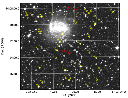
Figure 1: The field of SN 2013aa and SN 2017cbv. The image was taken on the du Pont telescope using the direct CCD camera through the $B$ filter. The locations of the two SNe are labeled in red. The local sequence stars are plotted as yellow circles and labeled with their identification numbers. North is up, East is to the left.

2.1 Photometry

SN 2013aa was observed as part of the Carnegie Supernova Project II (Phillips et al., 2019; Hsiao et al., 2019, hereafter CSP-II). Optical imaging was obtained with the Swope telescope equipped with the direct SITe3 CCD imager and a set of $ugriBV$ filters. NIR photometry was obtained using the 2.5-meter du Pont telescope with a set of $YJH$ filters. The observing procedures, data reduction, and photometric systems are outlined in other CSP papers (Krisciunas et al., 2017; Phillips et al., 2019).

SN 2017cbv was observed as part of the Swope Supernova Survey (Coulter et al., 2017, Rojas-Bravo et al., in prep). Similar to SN 2013aa, optical photometry was also obtained on the Swope telescope with the direct camera, but with an upgraded e2V CCD, which has been fully characterized by the CSP-II (Phillips et al., 2019). While the surveys employed slightly different strategies for target selection, this does not affect the observations presented here. The exact pointings for SN 2013aa and SN 2017cbv observations differ slightly to position each SN near the center of a chip. However because of the large Swope field of view, there are typically 25 local standard stars in common between the images, which we use to calibrate all SN photometry.

We emphasize that the optical photometry of both SNe and the NIR photometry of SN 2013aa are given in the CSP natural system. Using a long temporal baseline of observations at LCO, the CSP has determined the color terms that transform the instrumental magnitudes obtained on the Swope and du Pont telescopes into the standard magnitudes of Landolt (1992) ($BV$), Smith et al. (2002) ($ugri$), Persson et al. (1998) ($JH$) and Krisciunas et al. (2017) (Y). Using these color terms in reverse, we produce natural system magnitudes of our standards and local sequence stars, which are then used to differentially calibrate the photometry of each SN. This greatly simplifies the procedure of transforming to another photometric system so long as the filter functions used to obtain science images are accurately measured.

The NIR photometry of SN 2017cbv was obtained by Wee et al. (2018) using ANDICAM on the SMARTS 1.3-meter telescope at the Cerro Tololo Inter-American Observatory (CTIO). They used standard observing procedures, and tied their optical and NIR SN photometry to a single local sequence star. Comparing our $B$- and $V$-band photometry after computing S-corrections (Stritzinger et al., 2002), we note a systematic difference of order 0.1 – 0.2 mag, our photometry being dimmer. This appears to stem from the photometry of their single local sequence star (star 1 in Wee et al. 2018, star W1 in Figure  1), which is very red ($B-V=1.2$ mag) and comparatively bright ($V\sim 13$ mag). The red color leads to a relatively large color-term correction to transform the instrumental magnitude to standard and may introduce a large systematic error. In fact, this star is bright enough to be saturated in all but our shallowest exposures, so was not used to calibrate the Swope photometry. SN2017cbv was also observed independently with ANDICAM by a separate group and we find their data to be in agreement with the CSP data (Wang et al, in preparation).

The local sequence star used by Wee et al. (2018) to calibrate the NIR photometry, in contrast, has colors more consistent with the Persson et al. (1998) standards ($J-H\sim 0.3$ mag). Furthermore, they have used the CSP-I $Y$-band calibration from Krisciunas et al. (2017), with no color term applied, making their $Y$-band photometry nearly identical to the CSP natural system, differing only in the shapes of the $Y$ bandpasses. Unfortunately, there is no overlap between our RetroCam and the ANDICAM fields, making a direct comparison of local sequence stars impossible.

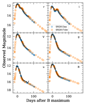
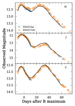
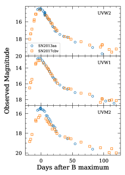
Figure 2: Optical, NIR and UV light curves of SN 2013aa and SN 2017cbv. The blue points correspond to SN 2013aa and the orange points correspond to SN 2017cbv. The NIR photometry of SN 2017cbv was obtained from images taken with ANDICAM. The UV points are from SWIFT. The solid black curves are SNooPy fits to SN 2013aa.

Lastly, the Neil Gehrels Swift Observatory observed both SN 2013aa and SN 2017cbv as part of the The Swift Optical/Ultraviolet Supernova Archive (SOUSA; Brown et al. 2014). Details of the photometric data reduction and calibration are given in Brown et al. (2009).

Table 1: A log of the visual-wavelength and NIR spectra presented in this work.

SN	$T_{spec}$	Phase	Instrument/Telescope
	JD$-$2,400,000	days
Optical
SN 2013aa	56339.4	$-$3.8	MIKE/Magellan
SN 2017cbv	57888.3	+47.7	MIKE/Magellan
SN 2017cbv	57853.5	$+$13.0	WiFeS/ANU 2.3-m
SN 2017cbv	57890.5	$+$50.0	WiFeS/ANU 2.3-m
NIR
SN 2013aa	56357.90	+14.7	FIRE/Baade
SN 2017cbv	57857.64	+17.1	FIRE/Baade

2.2 Spectroscopy

Visual-wavelength spectra of SN 2017cbv were obtained from Hosseinzadeh et al. (2017a), while those of SN 2013aa come from WISeREP (Yaron & Gal-Yam, 2012), with the exception of two spectra that were obtained with WiFeS (Dopita et al., 2007). WiFeS is an Integral Field Unit (IFU) on the 2.3-meter Australian National University telescope located at the Siding Spring Observatory. The WiFeS IFU has a $25\times 38$ arcsec field of view. Two gratings were used, for the blue and red cameras respectively, with a resolution of $R=3000$ along with a dichroic at 5600 Å. The data were reduced using pyWiFeS (Childress et al., 2014). The spectra were color-matched to the multi-band photometry to ensure accurate flux calibration.

We also present NIR spectra of both SN 2013aa and SN 2017cbv obtained with the FIRE spectrograph on the 6.5-meter Magellan Baade telescope at LCO. The spectra were reduced and corrected for telluric features following the procedures described by Hsiao et al. (2019). Additionally, high-resolution spectra of SN 2013aa and SN 2017cbv were obtained using the Magellan Inamori Kyocera Echelle (MIKE; Bernstein et al., 2003). The data were reduced using the MIKE pipeline (Kelson, 2003) and procedures outlined in Simon et al. (2010). A journal of spectroscopic observations is provided in Table 1.

3 Results

We present here the analysis of the data from the previous section, including photometric classification and the distances derived from common template light curve fitters. The spectra are used to delve into the physical characteristics of the explosions and progenitors.

Table 2: Comparison of LC parameters

Parameter	SN 2013aa	SN 2017cbv
Spline Fits
$t_{Bmax}$ (MJD)	56343.20(07)	57840.54(15)
$\Delta m_{15}(B)$ (mag)	0.95(01)	0.96(02)
$s^{D}_{BV}$	1.11(02)	1.11(03)
$B_{max}$	11.094(003)	11.118(011)
$V_{max}$	11.143(004)	11.173(010)
$B_{max}-V_{max}$	-0.048(005)	-0.056(015)
SNooPy
$t_{Bmax}$ (MJD)	56343.42(34)	57840.39(34)
$s_{BV}$	1.00(03)	1.12(03)
$E(B-V)$ (mag)	-0.03(06)	0.03(06)
$A_{V}$ (mag)	-0.06(12)	0.06(12)
$\mu$ (mag)	30.47(08)	30.46(08)
MLCS2k2
$t_{Bmax}$ (MJD)	56343.40(11) days	57839.79(06)
$\Delta$ (mag)	-0.09(02)	-0.26(02)
$A_{V}$ (mag)	-0.04(05)	0.23(05)
$\mu$ (mag)	30.56(04)	30.46(04)
SALT2
$t_{max}$ (MJD)	56343.95(03)	57840.66(03)
$x_{0}$	0.71(0.01)	0.61(0.01)
$x_{1}$	0.01(02)	1.30(17)
$c$ (mag)	-0.20(02)	-0.02(03)
$B_{max}$ (mag)	11.01(02)	11.17(03)
$\mu$ (mag)	30.62(04)	30.39(06)

Note. — All magnitudes and colors are corrected for Milky-Way extinction $E(B-V)=0.15$ mag based on Schlafly & Finkbeiner (2011).

3.1 Decline Rate

Figure 2 presents a comparison of the photometry of SN 2013aa and SN 2017cbv obtained with the Swope, du Pont, SMARTS, and Swift telescopes. The light curves of the two objects are remarkably similar, suggesting their progenitors could also be very similar. Table 2 lists pertinent photometric parameters estimated via the methods described below.

The most straightforward photometric diagnostic to compare is the light curve decline-rate parameter $\Delta m_{15}(B)$ (Phillips, 1993). Using the light curve analysis package SNooPy (Burns et al., 2011), the photometry is interpolated at day 15 in the rest frame of the SNe after applying K-corrections (Oke & Sandage, 1968) and time dilation corrections. This results in nearly the same decline rate $\Delta m_{15}(B)\simeq 0.95$ mag, indicating both objects decline slightly slower than the typical $\Delta m_{15}(B)$ value of 1.1 mag (Phillips et al., 2019, Fig. 10).

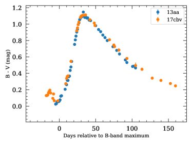
Figure 3: The $B-V$ color-curve evolution of SN 2013aa and SN 2017cbv. The time of $B-V$ maximum relative to $B$-band maximum divided by 30 days is defined as the color stretch, $s^{D}_{BV}$, which is nearly identical for these two SNe.

Another way to characterize the decline-rate of the SNe directly from photometry is to measure the epoch that the $B-V$ color-curves reaches their maximum point (i.e., when they are reddest) in their evolution relative to the epoch of $B$-band maximum. Dividing by 30 days gives the observed color-stretch parameter $s^{D}_{BV}$. Burns et al. (2014) showed that the color-stretch parameter was a more robust way to classify SNe Ia in terms of light curve shape, intrinsic colors and distance (Burns et al., 2018). Figure 3 shows the $B-V$ color-curves for SN 2013aa and SN 2017cbv. Fitting the $B-V$ color-curves with cubic splines, we find identical color-stretch values of $s^{D}_{BV}=1.11$ for both objects, again making them slightly slower than typical SNe Ia.

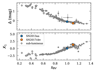
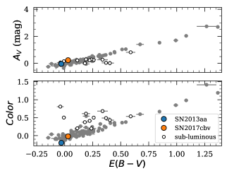
Figure 4: Comparison of parameters from three different SN Ia light curve fitters for the CSP-I sample. (Left) Comparing the shape parameters, the MLCS2k2 parameter $\Delta$ (top panel) and SALT2 parameter $X_{1}$ (bottom panel) are plotted versus the SNooPy color-stretch parameter $s_{BV}$. (Right) Comparing color/reddening parameters, the MLCS2k2 parameter $A_{V}$ (top panel) and SALT2 color parameter (bottom panel) are plotted versus the SNooPy $E(B-V)$ parameter. SN 2013aa and SN 2017cbv are labeled with blue and orange circles, respectively.

For the purposes of determining distances for cosmology, it is more common to fit multi-band photometry simultaneously, deriving a joint estimate of the decline rate, color/extinction, and distance. To this end, the light curves of both SNe Ia are fit with 3 light curve fitting methods: 1) SNooPy, 2) SALT2 (Guy et al., 2007), and 3) MLCS2k2 (Jha et al., 2007). The results of these fits are listed in Table 2. In terms of the decline rate, a slightly different picture emerges: all three fitters classify SN 2013aa as a faster decliner than SN 2017cbv. In Figure 4 we show how the different decline-rate parameters (SNooPy’s $s_{BV}$, SALT2’s $x_{1}$, and MLCS2k2’s $\Delta$) relate to each other for the CSP-I sample (Krisciunas et al., 2017). It is clear that the three decline rate parameters for the two SNe follow the general trend and are therefore measuring the same subtle differences in light-curve shapes that tell us SN 2013aa is a faster decliner, despite having nearly identical $\Delta m_{15}(B)$ and $s^{D}_{BV}$. This is because $\Delta m_{15}(B)$ is determined from only two points on the $B$ light curve (maximum and day 15) and $s^{D}_{BV}$ is determined from one point on the $B$ light curve and one point on the $B-V$ color curve, whereas template fitters like SNooPy, MLCS2k2 and SALT2 use the shapes of multi-band light curves to determine the decline rates. Looking closely at the color-curves of both SNe in Figure 3, while the peaks are nearly identical, SN 2017cbv rises more quickly prior to maximum and declines more slowly after maximum.

3.2 Extinction

Both SN 2013aa and SN 2017cbv are located in the outer parts of NGC 5643 on opposite sides, having a host offset of 17 kpc and 14 kpc, respectively. We therefore expect minimal to no host-galaxy dust reddening for either object. However, NGC 5643 is at a relatively low galactic latitude ($l=15.03$°) with a predicted Milky-Way color excess of $E(B-V)_{MW}=0.15$ mag (Schlafly & Finkbeiner, 2011).

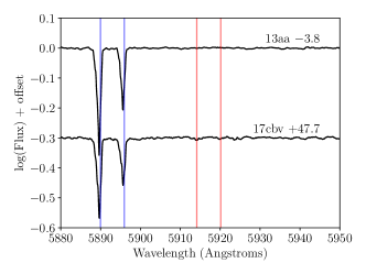
Figure 5: Continuum-normalized MIKE spectra of SN 2013aa and SN 2017cbv in the vicinity of the Na idoublet. Absorption from the Milky-Way is clearly visible. The blue vertical lines denote the rest wavelengths of the Na I D2 $5890$ Å and Na I D1 $5896$ Å lines, and the red lines show their location red-shifted to the systemic velocity of NGC 5643, i.e., 1200 kms. The names and phases of the spectra relative to the epoch of peak brightness are indicated to the right of each spectrum.

Figure 5 shows the continuum-normalized spectra of SN 2013aa and SN 2017cbv taken with MIKE in the Na I D region. Absorption from the Milky-Way is clearly visible in both cases, while absorption at the systemic velocity of NGC 5643 is only detected in the spectrum of SN 2017cbv. Measuring the equivalent width of the combined Na I D lines and using the conversion from Poznanski et al. (2012), we obtain an average Milky-Way reddening of $E(B-V)_{MW}=0.23\pm 0.16$ mag, somewhat higher than the Schlafly & Finkbeiner (2011) value, but within the uncertainty. The equivalent width of the host Na I D corresponds to $E(B-V)_{host}=0.015\pm 0.010$ mag. While the strength of Na I D absorption has been shown to be a poor predictor of the amount of extinction in SN Ia hosts, the absence of Na I D nevertheless seems to be a reliable indicator of a lack of dust reddening (Phillips et al., 2013). In the remainder of this paper the Schlafly & Finkbeiner (2011) value is adopted for the Milky-Way reddening along with a reddening law characterized by $R_{V}=3.1$, in order to correct the SN photometry for the effects of Milky-Way dust.

The photometric colors of both objects are very blue at maximum, with SN 2017cbv being only slightly bluer. However, when the correlation between intrinsic color and decline rate (e.g. Burns et al., 2014) is taken into account, one infers slightly more extinction in SN 2017cbv than SN 2013aa. SALT2, which does not estimate the extinction but rather a rest-frame color parameter, gives a bluer color ($c=-0.20$) for SN 2013aa than for SN 2017cbv ($c=-0.02$). In fact, as can be seen in Figure 4, SN 2013aa’s color parameter is lower than our entire CSP-I sample. MLCS2k2 provides estimates of the visual extinction, $A_{V}$, and gives a significant host extinction for SN 2017cbv ($A_{V}=0.23\pm 0.05)$ mag, or $E(B-V)=0.12\pm 0.03$ mag. However, like SNooPy, MLCS2K2 K-corrects its template light curves to fit the CSP filters and our $u$ band is significantly different from Johnson/Cousins $U$, resulting in rather large corrections. Eliminating $u$ from the fit brings the extinction estimate down to $A_{V}=0.12\pm 0.06$ mag or $E(B-V)=0.06\pm 0.03$ mag, consistent to within the errors with the SNooPy value.

Given the positions of the two SNe, their lack of Na I D absorption at the velocity of the host, and that SNooPy predicts zero color excess, we conclude that SN 2013aa and SN 2017cbv experience minimal to no significant host-galaxy dust extinction, making them ideal objects to improve upon the zero-point calibration of SNe Ia.

3.3 UV Diversity

An outstanding feature of Figure 2 is the difference at peak in the single Swift band $UVM2$ while the two other filters, $UVW1$ and $UVW2$, are consistent. This is likely due to the fact that both $UVW1$ and $UVW2$ have significant red leaks and nearly 50% of the flux comes from the optical light. $UVM2$ is therefore a better indicator for diversity in the UV, sampling the wavelength region $2000-3000$ Å.

Figure 6 shows the $UVW1-v$ and $UVM2-v$ colors as a function of time for SN 2013aa and SN 2017cbv, as well as the two “twins” SN 2011fe and SN 2011by. Two shaded regions are also shown indicating two populations of SNe Ia: the NUV-blue and NUV-red as defined by Milne et al. (2013). They would seem to indicate that both SN 2013aa and SN 2017cbv are NUV-blue. However, when comparing the $UVM2-v$ colors, there is much more diversity and while SN 2013aa is similar to SN 2011by, SN 2017cbv is much redder and SN 2011fe is much bluer, particularly near maximum light. This underscores the issues with the red leaks. Milne et al. (2013) attribute these differences in NUV colors to differences in how close the burning front reaches the surface of the ejecta. Alternatively, near-UV differences may be the result of varied metal content in the ejecta (e.g, Walker et al., 2012; Brown et al., 2019), though no correlation has been found between the near-UV and the host galaxy metallicity (Pan et al., 2019; Brown & Crumpler, 2019).

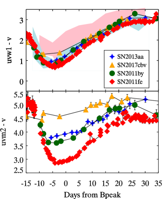
Figure 6: A comparison of the SWIFT UVOT $UVW1-V$ and $UVM2-v$ color curves. SN 2013aa, SN 2017cbv, and the twins SN 2011fe and SN 2011by are plotted with symbols. The red and blue shaded regions in the upper panel delimit the NUV-red and NUV-blue regions from Milne et al. (2013), respectively.

3.4 Spectroscopy

3.4.1 Optical

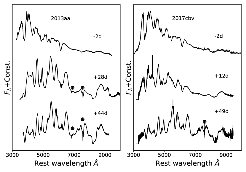
Figure 7: A rest frame time series of spectra for SN 2013aa (left) and SN  2017cbv (right). Phases are given relative to $B$-band maximum. Telluric regions in the spectra are marked.

Figure 7 presents our spectral time series of SN 2013aa and SN 2017cbv. Only data obtained during the photospheric and transitional phase are shown as the nebular phase spectra will be the highlight of a future study. In the case of both objects, three optical spectra were obtained starting at $-2$ d with respect to $B$-band maximum. The last spectra of SN 2013aa and SN 2017cbv were obtained on +44 d and +49 d, respectively.

Doppler velocities and pseudo-EW (pEW) measurements were calculated for each object by fitting the corresponding features with a Gaussian function. The range over which the data were fit was manually selected, and the continuum in the selected region was estimated by a straight line. The velocity was then measured by fitting the minimum of the Gaussian and the error was taken as the formal error of the Gaussian fit. Finally, pEW measurements were obtained following the method discussed in Garavini et al. (2007).

The spectra of the SNe are characteristic of normal SNe Ia. The $-2$ d Si II $\lambda$6355 Doppler velocity of SN 2013aa and SN 2017cbv are $-$10,550$\pm$30km s^-1and $-$9,800$\pm$20km s^-1, respectively. This places them both as normal-velocity SN Ia in the Wang et al. (2013) classification scheme. They are also both core normal (CN) in the Branch et al. (2006) classification system, as demonstrated in the Branch diagram plotted in Figure 8. Although the two objects are located close to the boundary between CN and shallow silicon (SS) SNe Ia.

Figure 9 shows a comparison of the spectra of the two SNe obtained at early ($-2$ d) and later ($+44$ d and $+49$ d) phases. At $-2$ d the spectra are nearly identical, exhibiting very similar line ratios and ionization structures. They contain classic broad P Cygni-like features typical of SNe Ia. They are also both dominated by doubly and singly ionized species, all of which are labeled in Figure 9. The main difference between the two objects at $-2$ d is the width of the Si II $\lambda$6355 feature, where SN 2013aa (EW=84$\pm$1Å) is broader than SN 2017cbv (EW=76$\pm$1Å). This suggests that SN 2013aa has a more extended Si region. The spectra of SN 2013aa and SN 2017cbv also look remarkably similar at +44 d and +49 d, respectively. At these epochs there is no longer a definitive photosphere and emission lines begin to emerge in the spectra.

It has been hypothesized that using ‘twin’ SN Ia can improve their use as distance indicators (Fakhouri et al., 2015). Given their photometric similarity, a natural question to address is to what degree are SN 2013aa and SN 2017cbv spectroscopic twins? Following the definition of single phase twinness by Fakhouri et al. (2015), we compute their $\xi(p_{i})$ parameter using the $-2$ d spectra of both objects. $\xi$ is essentially a reduced $\chi^{2}$ statistic and therefore requires a good noise model that we estimate by boxcar-averaging each spectrum with a box size of 11 wavelength bins and subtracting these smoothed spectra from the originals. We also color-match each spectrum to match the observed photometry and only consider the wavelength range (4000–9500 Å), corresponding to the wavelength coverage of our $BVri$ photometry. The resulting value of $\xi(-2)=1.7$ corresponds to 70% in the cumulative distribution from Fakhouri et al. (2015). In other words, 70% of SNe Ia from their sample have a $\xi$ of 1.7 or less, indicating SN 2013aa and SN 2017cbv are not spectroscopic twins by this metric. We note, however, that the two spectra were obtained on different instruments. This could introduce systematic errors that are not accounted for in the noise model and could lead to an over-estimate of $\xi$.

3.4.2 NIR

NIR spectra of SN 2013aa and SN 2017cbv obtained at $+14.5$ d and +17.1 d, respectively, are plotted in Figure 10. The spectra are very similar, and are dominated by lines of iron group elements (see line IDs in the figure). A prevalent emission feature in the $H$-band region emerges in all SNe Ia by $+10$ d linked to allowed emission lines of Co ii, Fe ii and Ni ii  produced from the radioactive decay of ⁵⁶Ni which is located above the photosphere (Wheeler et al., 1998; Hsiao et al., 2015). Ashall et al. (2019a) found a correlation between the the outer blue-edge velocity, $v_{edge}$, of this $H$-band break region and s_BV. Furthermore, Ashall et al. (2019b) found that $v_{edge}$ was a direct measurement of the sharp transition between the incomplete Si-burning region and the region of complete burning to ⁵⁶Ni. $v_{edge}$  measures the ⁵⁶Ni mass fraction between 0.03 to 0.10.

Using the method of Ashall et al. (2019a), $v_{edge}$ is measured from the NIR spectra of both objects. At $+14.4$ d, SN 2013aa had a $v_{edge}$ of $-$13,600$\pm$300km s^-1, and at $+17.1$ d SN 2017cbv had a $v_{edge}$ of $-$12,300$\pm$400km s^-1. SN 2017cbv has a lower value of $v_{edge}$ by 1300km s^-1, however this is likely to be due to the fact that $v_{edge}$ decreases over time (see Ashall et al., 2019a).

The fact that both SNe have similar values of $v_{edge}$ and absolute magnitude indicates that they probably have a very similar total ejecta mass. As explained in Ashall et al. (2019b), for a given ⁵⁶Ni mass, smaller ejecta masses produce larger values of $v_{edge}$. However, $v_{edge}$ is similar in both SN 2017cbv and SN 2013aa, once the phase difference in the spectra is taken into account. Furthermore, the value of $v_{edge}$ obtained from SN 2017cbv is consistent with similar SNe from Ashall et al. (2019a), as well as with predictions of Chandrasekhar mass ($M_{Ch}$) delayed-detonation explosion models (Hoeflich et al., 2017; Ashall et al., 2019b). It should be noted that in Ashall et al. (2019a) and Ashall et al. (2019b) the time period to measure $v_{edge}$ was given as 10$\pm$3 d. However for normal-bright SNe Ia the change in $v_{edge}$ is slow, hence comparing to spectra at $+14.4$ d is still appropriate.

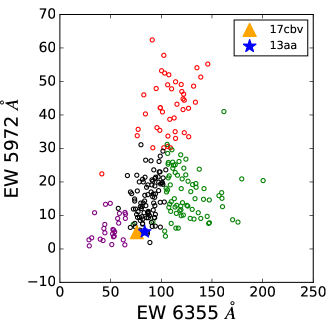
Figure 8: The Branch diagram for SNe Ia. SN 2013aa (blue star) and SN  2017cbv (orange triangle) are overlaid. The shallow silicon (purple), core normal (black), broad line (green) and cool line (red) SNe are plotted from Blondin et al. (2012).

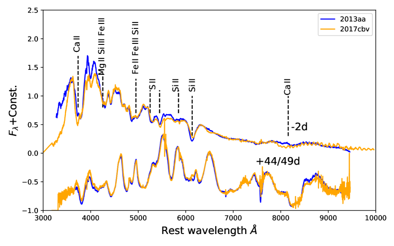
Figure 9: A comparison of the optical spectra of SN 2013aa and SN 2017cbv at two epochs. Phases are given relative to $B$-band maximum.

4 Progenitors

SNe Ia are thought to originate from the thermonuclear disruption of Carbon-Oxygen (C-O) white dwarfs (WD) in binary systems. There are many popular progenitor and explosions scenarios (see Livio & Mazzali, 2018, for a recent review). Two of the favored explosion scenarios, which can occur in both the single and double degenerate progenitor system, are the double detonation (He-det) and delayed detonation scenarios (DDT). In the He-det scenario a sub-$M_{Ch}$ WD accretes He from a companion, either a He star or another WD with a He layer, the surface He layer detonates and drives a shock wave into the WD producing a central detonation (Livne & Arnett, 1995; Shen & Moore, 2014; Shen et al., 2018). In the DDT scenario, a WD accretes material until it approaches the $M_{Ch}$, after which compressional heating near the WD center initiates a thermonuclear runaway, with the burning first traveling as a subsonic deflagration wave and then transitions into a supersonic detonation wave.

It has been predicted that SNe Ia spectra can look similar at maximum light, and their light curves can have the same shape, but their absolute magnitudes can differ by $\sim$0.05 mag (Hoeflich et al., 2017). This should be the case for both He-det (assuming the ejecta masses are similar) and DDT explosions. This is because at early times one of the dominant processes is how the ⁵⁶Ni heats the photosphere; that is, where the ⁵⁶Ni is located with respect to the photosphere. However, once the photosphere is within the ⁵⁶Ni region the exact location of the ⁵⁶Ni  can differ and alter the light curve and spectra after 30 days past maximum light (Hoeflich et al., 2017).

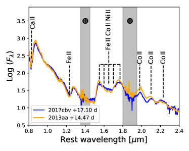
Figure 10: A spectral comparison between SN 2013aa and SN 2017cbv in the NIR, at two different epochs. Phases are given in the legend.

Figure 3 shows that the $B-V$ color curves for both objects are very similar. Furthermore, the optical spectra of SNe 2013aa and 2017cbv are nearly identical at $\sim$+43 d when the photosphere is well within the ⁵⁶Ni region. This demonstrates that these two objects are similar in the inner regions, and have similar ignition mechanisms. However, at $-2$ d the spectrum of SN 2013aa has a broader Si II $\lambda$6355 feature indicating that it has more effective burning and a larger intermediate mass element (IME) region. This implies that any small differences between the two objects is in the outer layers. This could potentially be caused by differences in the main sequence mass of the star before it produces the WD, which changes the C to O ratio and the effectiveness of the burning in the outer layers (Hoeflich & Khokhlov, 1996; Hoeflich et al., 2017; Shen et al., 2018). This would alter the region between explosive oxygen and incomplete Si burning in the ejecta, but not change the total ⁵⁶Ni production and hence the luminosity, as is seen with the extended Si region in SN 2013aa. However, overall it is likely that the explosion mechanism for both objects is very similar, and the observations of these SNe are largely consistent with the DDT and/or He-Det scenarios.

5 Distance

Table 3: SN Ia siblings in the literature.

Host	SN	$s_{BV}$	$E(B-V)$	$\mu$	$\Delta\mu$	Photometric system reference
			mag	mag	mag
NGC 105	SN1997cw	1.30(04)	0.29(07)	34.34(11)		CfA
	SN2007A	1.01(04)	0.24(06)	34.38(10)	0.04(15)	CfA
	SN2007A	1.10(02)	0.24(06)	34.44(11)	0.10(17)	CSP
NGC 1316	SN2006mr	0.25(03)	0.03(04)	31.26(04)		CSP (Burns et al., 2018)
	SN1980N	0.88(03)	0.14(06)	31.27(09)	0.01(10)	CTIO 1m - photographic
	SN2006dd	0.93(03)	0.09(06)	31.29(09)	0.03(10)	ANDICAM (Stritzinger et al., 2010)
	SN1981D	0.77(05)	0.05(09)	31.32(10)	0.06(11)	CTIO 1m
NGC 1404	SN2011iv	0.64(03)	$-$0.05(06)	31.18(09)		CSP
	SN2007on	0.58(03)	$-$0.06(06)	31.59(10)	0.41(13)	CSP (Gall et al., 2018).
NGC 1954	SN2013ex	0.92(03)	$-$0.01(06)	33.64(09)		Swift UVOT
	SN2010ko	0.57(04)	$-$0.07(07)	33.92(14)	0.28(17)	Swift UVOT
NGC 3190	SN2002cv	0.85(04)	5.40(09)	31.91(61)		Standard (Elias-Rosa et al., 2008)
	SN2002bo	0.89(03)	0.40(06)	32.03(13)	0.12(62)	CfA
	SN2002bo	0.94(03)	0.43(06)	32.11(13)	0.20(62)	KAIT
	SN2002bo	0.92(03)	0.42(06)	32.11(14)	0.20(63)	Standard + LCO NIR (Krisciunas et al., 2004)
NGC 3905	SN2009ds	1.05(03)	0.07(06)	34.69(09)		CfA, PAIRITEL
	SN2001E	1.02(04)	0.47(06)	34.85(14)	0.16(17)	KAIT
NGC 4493	SN2004br	1.12(04)	0.01(06)	34.82(08)		KAIT
	SN1994M	0.88(04)	0.17(06)	35.07(09)	0.25(12)	CfA (Riess et al., 1999)
NGC 4708	SN2016cvn	1.25(12)	0.91(13)	33.71(24)		Foundation (Foley et al., 2018b)
	SN2005bo	0.79(03)	0.28(06)	33.95(11)	0.24(26)	CSP
	SN2005bo	0.86(03)	0.37(06)	33.96(12)	0.25(27)	KAIT
NGC 5468	SN1999cp	0.98(03)	0.06(06)	33.10(08)		KAIT, 2MASS, (Krisciunas et al., 2000)
	SN2002cr	0.91(03)	0.11(06)	33.17(08)	0.07(11)	KAIT
	SN2002cr	0.93(03)	0.10(06)	33.21(09)	0.11(12)	CfA
NGC 5490	SN2015bo	0.41(08)	0.11(13)	34.18(19)		Swift UVOT
	SN1997cn	0.62(04)	0.12(06)	34.57(10)	0.39(21)	CfA
NGC 5643	SN2017cbv	1.09(04)	0.08(06)	30.38(09)		Swift UVOT
	SN2013aa	0.95(03)	$-$0.03(06)	30.40(08)	0.02(12)	LCOGT (Graham et al., 2017)
	SN2017cbv	1.13(03)	0.03(06)	30.46(08)	0.08(12)	CSP (This work)
	SN2013aa	1.00(03)	$-$0.03(06)	30.47(08)	0.09(12)	CSP (This work)
	SN2013aa	1.05(03)	$-$0.01(06)	30.57(08)	0.19(12)	Swift UVOT
NGC 6240	PS1-14xw	0.95(04)	0.26(06)	34.79(12)		Swift UVOT
	SN2010gp	1.06(07)	0.00(07)	35.22(12)	0.43(17)	Swift UVOT
NGC 6261	SN2008dt	0.87(05)	0.49(09)	35.85(18)		CfA
	SN2008dt	0.81(05)	0.14(07)	35.87(15)	0.02(23)	KAIT
	SN2007hu	0.80(05)	0.39(08)	35.91(14)	0.06(22)	CfA
UGC 3218	SN2011M	0.93(02)	0.08(06)	34.37(08)		KAIT
	SN2011M	0.85(05)	$-$0.01(07)	34.37(10)	0.00(14)	Swift UVOT
	SN2006le	1.08(04)	$-$0.03(06)	34.44(08)	0.07(13)	KAIT
	SN2006le	1.20(03)	$-$0.11(06)	34.61(10)	0.24(13)	CfA, PAIRITEL
UGC 7228	SN2007sw	1.19(04)	0.14(07)	35.25(10)		CfA
	SN2012bh	1.11(04)	0.10(06)	35.39(09)	0.14(13)	PANSTARRS (Jones et al., 2018)

With a heliocentric redshift $z_{hel}=0.003999$ (Koribalski et al., 2004), NGC 5643 is close enough to have its distance determined independently, adding to the growing number of hosts that can be used to calibrate the SN Ia distance ladder for the purpose of determining the Hubble constant. And being siblings, SN 2013aa and SN 2017cbv provide a consistency check on the reliability of SN Ia distances in general. Using the Burns et al. (2014) calibration of the Phillips relation and the light-curve parameters from SNooPy, we find distances of $\mu=30.47\pm 0.08$ mag and $\mu=30.46\pm 0.08$ mag for SN 2013aa and SN 2017cbv, respectively. The difference in distance modulus is $0.01\pm 0.11$, and therefore is insignificant. This compares well with the distance determined by Sand et al. (2018), who used MLCS2k2 on their own photometry to derive a distance of $\mu=30.45\pm 0.09$. MLCS2k2 infers a distance of $\mu=30.56\pm 0.08$ mag for SN 2013aa and $\mu=30.46\pm 0.08$ for SN 2017cbv, which is a difference of $0.10\pm 0.11$ mag, so within the uncertainty of the fitter. SALT2, however, infers distances of $\mu=30.62\pm 0.11$ for SN 2013aa and $\mu=30.39\pm 0.12$ for SN 2017cbv, a difference of $0.23\pm 0.16$ mag. The larger differences for SALT2 and MLCS2k2 are primarily due to differences in their color parameters (MLCS2k2 inferring SN 2017cbv to have significant $A_{V}$ and SALT2 inferring SN 2013aa to have very blue color).

Table 3 gives a list of the current sample of SNe Ia siblings in the literature. Using SNooPy, we have derived decline rates, extinctions and distance estimates to each object. We then compare the inferred host distances, which are tabulated in the column labeled $\Delta\mu$. In all, it was found that 14 host galaxies have hosted two SNe Ia and one (NGC 1316) has hosted 4 SNe Ia. The differences in distance estimate range from 0.02 mag to 0.43 mag.

Of particular interest are the siblings that were observed with the same telescopes and instruments, eliminating the systematic error of transforming photometry from one system to another (Stritzinger et al., 2005). In this regard, Swift shows the greatest dispersion among siblings with $\Delta\mu=0.43$ mag for NGC 6240 and $\Delta\mu=0.28$ mag for NGC 1954. In the case of NGC 6240, the two SNe have color excesses that differ by 0.26 mag and only the UVOT $B$ and $V$ filters could be reliably fit with SNooPy, requiring we assume the typical $R_{V}=2$ for SNe Ia (Mandel et al., 2009; Burns et al., 2014), rather than fit for it using multi-band photometry. If $R_{V}$ is in fact higher by an amount $\Delta R_{V}$ for this host, the discrepancy would decrease by $\simeq 0.26\cdot\Delta R_{V}$. As a result, if $R_{V}$ were as high as 4 in NGC 6240, the discrepancy would be eliminated. In the case of NGC 1954, SN 2010ko is a transitional Ia (Hsiao et al., 2013) which have been shown to be less reliable as standard candles (see discussion of NGC 1404 below). This is also true of NGC 5490, in which both SNe are transitional.

Further investigation comparing Swift and CSP photometry has also shown systematic errors between some SNe in common which can be as high as 0.15 mag. Comparing the UVOT photometry of local sequence stars during the separate observing campaigns of the sibling SNe does not show a significant difference (N. Crumpler, private communication). The Swift sibling SNe are also not located near bright stars or in bright regions of the host which can invalidate the standard non-linearity corrections (Brown et al., 2014). Further investigation of these discrepancies is ongoing.

The Lick Observatory Supernova Search (LOSS) observed two pairs of siblings in NGC 5468 and UGC 3218 using the Katzman Automatic Imaging Telescope (KAIT). Both pairs (SN 1999cp/SN 2002cr and SN 2006le/SN 2011M) exhibit similar decline rates and both pairs had low reddening. The distance estimates for NGC 5468 differ by less than the error ($\Delta\mu=0.07\pm 0.11$), as is the case for UGC 3218 ($\Delta\mu=0.07\pm 0.13$). However, in other hosts where data were taken with different telescopes, the KAIT distances tend to differ by $\Delta\mu\sim 0.2$ mag. LOSS publish their photometry in the standard system (Silverman et al., 2012), which is known to introduce systematic errors that are difficult to correct and could be the cause of the larger discrepancy (Stritzinger et al., 2002).

The CfA supernova survey observed two pairs of siblings: one in NGC 6261 (SN 2008dt and SN 2007bu) and another in NGC 105 (SN 1997cw and SN 2007A). In both cases, the difference in the inferred distance is well under the uncertainties ($\Delta\mu=0.06\pm 0.22$ mag and $\Delta\mu=0.04\pm 0.15$ mag respectively). In particular, both SN 2007A and SN 1997cw have moderately high reddening $E(B-V)_{host}\sim 0.3$ mag, yet agree to within 2%. Again, however, when comparing siblings observed with different photometric systems, the differences tend to be larger.

Lastly, prior to this paper, the CSP studied one pair of siblings in the host NGC 1404, namely SN 2007on and SN 2011iv (Gall et al., 2018). The difference in distance modulus obtained from the two objects was $\Delta\mu=0.41$ mag, which is quite large for objects observed with the same facilities and hosted in the same galaxy. However, both objects have transitional decline rates placing them between normal SNe Ia ($s_{BV}>0.6$) and fast-decliners ($s_{BV}<0.4$), and it is likely that physical differences in their progenitors are responsible for their different peak luminosities (Gall et al., 2018).

It is also worth re-examining NGC 1316 (Fornax A), which hosted 4 SNe Ia. These were previously analyzed by Stritzinger et al. (2010), who found that the three normal SNe Ia (SN 1980N, SN 1981D, and SN 2006dd) all agreed to within 0.03 mag, but the extremely fast-declining SN 2006mr disagreed by nearly a magnitude. This analysis was done using $\Delta m_{15}(B)$ as a light curve decline-rate parameter, which was later shown to fail for fast-declining SN Ia (Burns et al., 2014). Using $s_{BV}$ instead leads to a SN 2006mr distance that is in complete agreement with the other normal SNe Ia (Burns et al., 2018). This is the distance tabulated in Table 3. We therefore have siblings in NGC 1404 that seem to indicate fast (or at least transitional) decliners are not as reliable, while NGC 1316 would indicate they are. If there is a diversity in progenitors at these decline rates, then we may simply be seeing an increased dispersion in the Phillips relation at the low $s_{BV}$ (high $\Delta m_{15}(B)$) end, or perhaps two different progenitor scenarios. To know for sure will require an expanded sample of transitional SNe Ia.

Table 4: Intrinsic dispersions in the sibling distances.

Subsample	$\sigma_{SN}$	$N_{pair}$	$N_{gal}$
All pairs	$0.14(02)$	34	15
No Swift SNe	$0.07(03)$	28	12
$s_{BV}>0.6$	$0.12(02)$	25	12
$s_{BV}>0.6$ and No Swift SNe	$<0.03$ (95% conf.)	21	11

More quantitatively, we have 34 pairs of distances that can be compared, including multiple observations of the same SN Ia with different telescopes/ instruments. Using a simple Bayesian hierarchical model, we can solve for an intrinsic dispersion $\sigma_{SN}$ in these distances, taking into account the photometric errors, errors in the SN Ia calibration, and systematic errors due to different photometric systems (see appendix B for details of this modeling). Using all pairs, we derive $\sigma_{SN}=0.14\pm 0.02$, however this is dominated by the outliers mentioned above. If we eliminate the Swift observations, the intrinsic dispersion reduces to $\sigma_{SN}=0.07\pm 0.03$, or 3% in distance. If we further remove the fast declining SNe ($s_{BV}<0.6$), we obtain only an upper limit $\sigma_{SN}<0.03$ at 95% confidence. These results are summarized in Table 4.

Within this landscape, we present two normal SNe Ia siblings observed with the same telescope and nearly identical detector response functions. Unlike most of the siblings in Table 3, SN 2013aa and SN 2017cbv have dense optical and NIR coverage, allowing for accurate measurement of the extinction, which is found to be consistent with minimal to no reddening in both cases. The difference in distance modulus ($\Delta\mu=0.01$) is less than the uncertainties, as was the case with the CfA and KAIT siblings. Being at such low redshift, we can expect the SN Ia distances to differ from the Hubble distance modulus by about $\delta\mu=\frac{2.17v_{pec}}{cz_{hel}}=0.54$ mag for an assumed typical peculiar velocity of $v_{pec}=300\ \mathrm{km\ s^{-1}}$. With a CMB frame redshift $z_{cmb}=0.0047$ and assumed Hubble constant $H_{0}=72\ \mathrm{km\ s^{-1}\ Mpc^{-1}}$, the distance modulus is $\mu=31.44$ mag, nearly a magnitude larger. Applying velocity corrections for Virgo, the Great Attractor, and the Shapley supercluster decreases the distance modulus to $\mu=30.82$ mag. These differences in distance demonstrate the use of standard candles such as SNe Ia for determining departures from the Hubble expansion at low redshift. With a precision of 3% in distances, we can measure deviations from the Hubble flow at a level of $\delta v=0.03H_{0}d$. This corresponds to $\delta v\simeq 40\mathrm{km\ s^{-1}}$ at the distance of the Virgo cluster ($20$ Mpc) and $\delta v\simeq 220\mathrm{km\ s^{-1}}$ at the distance of Coma ($100$ Mpc).

6 Conclusions

The galaxy NGC 5643 is unique in that it has hosted two normal SNe Ia that have very similar properties and is close enough to have its distance determined independently. All photometric and spectroscopic diagnostics indicate that SN 2013aa and SN 2017cbv are both normal SNe Ia with minimal to no host-galaxy reddening. This is also consistent with their positions in the outskirts of the host galaxy. Both objects have been observed in the optical with the same telescope and instruments and show a remarkable agreement in their light curves.

Comparing the distances inferred by SN 2013aa and SN 2017cbv gives us the opportunity to test the relative precision of SNe Ia as standard candles without a number of systematics that typically plague such comparisons. Given that they occurred in the same host galaxy, there is no additional uncertainty due to peculiar velocities. Having been observed by essentially the same telescope and instruments with the same filter set, there is also minimal systematic uncertainty due to photometric zero-points or S-corrections. Finally, having no dust extinction, we eliminate the uncertainty due to extinction corrections and variations in the reddening law (Mandel et al., 2009; Burns et al., 2014). When fitting multi-band photometry using SNooPy, SALT2, and MLCS2k2, SN 2013aa is found to be characterized by a slightly faster decline rate and bluer color at maximum. The net result is a difference in distance that is insignificant compared to the measurement errors, a similar situation as the other pairs of normal siblings observed in multiple colors with the same instruments.

The similarity between the spectra and light curves of SN 2013aa and SN 2017cbv at all observed epochs suggest that they may have similar explosion mechanisms and progenitor scenarios. However the differences between most leading explosion models are best seen at early and late times. At these earliest epochs, SN 2017cbv showed an early blue excess, but there were no data for SN 2013aa. Naturally the question is then: would SN 2013aa also have shown this early blue excess? Although we cannot make this comparison for these two objects, it is something that could be studied in the future using SN siblings.

Some of the other questions that naturally arise for the future with twins and sibling studies are: if the spectral evolution were different, e.g. one SN was high velocity gradient, and the other low velocity gradient, or if the SNe were different spectral sub-types at maximum light (e.g. shallow silicon vs. core normal vs. cool) would the distance calculated for each SN be different and, if so, does this point to different explosion mechanisms and progenitor scenarios? Also, with the advent of Integral Field Spectrographs (IFS), we are beginning to study the local host properties (Galbany et al., 2018). Future IFS observations will allow us to investigate any correlation between these local properties and differences in inferred distance.

With the exception of the Swift siblings, which had limited wavelength coverage, we have four cases of normal SNe Ia where most of the systematic errors are absent and find the relative distance estimates to agree to within 3%. Another host, NGC 1316, shows the same kind of consistency despite having multiple photometric sources. This kind of internal precision rivals that of Cepheid variables (Persson et al., 2004). The picture is not as encouraging in the case of transitional- and fast-declining SNe Ia, and more examples of these types of objects in the Hubble flow and/or additional pairs of such siblings are required. Comparing siblings from multiple telescopes also shows that we can expect disagreements on order of 5% to 10%, higher than typical systematic errors in the photometric systems themselves. A likely reason for this is that these systematics in the photometric systems don’t just affect the observed brightness, but also the observed colors, which are multiplied by the reddening slope $R_{\lambda}$ when correcting for dust. It is therefore advantageous to use the reddest filters possible to avoid this systematic when determining distances to SNe Ia (Freedman et al., 2009; Mandel et al., 2009; Avelino et al., 2019).

After submission of this paper, Scolnic et al. (2020) released a preprint detailing the analysis of sibling SNe Ia from the DES survey. Unlike our results, they find the dispersion among siblings to be no less than the non-sibling SNe. Their sample, though, is quite different from ours. Their SNe are photometrically classified while ours are spectroscopically classified. They could therefore have peculiar SNe Ia in their sample. Theirs is also a higher redshift sample, ranging from $z=0.228$ to $z=0.648$. This results not only in larger errors due to k-corrections, but also the fact that they are measuring restframe wavelengths that are considerably bluer, on average, than ours. The errors in the color corrections will therefore be larger. It is also well-known that SNe Ia show more diversity in the near-UV and UV (Foley et al., 2008; Brown et al., 2017).

The analysis of sibling SNe gives us confidence that for appropriate cuts in decline rate and when using well-understood photometric systems, relative distances inferred from SNe Ia are on par with primary indicators such as Cepheid variables, but to greater distances.

Table 5: Natural system photometry of SN 2013aa and SN 2017cbv.

MJD	Filter	Magnitude	Phase
days		mag	days
SN2013aa
56338.360	$B$	$11.885$(006)	$-5.086$
56339.369	$B$	$11.811$(009)	$-4.078$
56340.384	$B$	$11.759$(007)	$-3.062$
56341.390	$B$	$11.707$(006)	$-2.056$
56342.386	$B$	$11.699$(006)	$-1.061$
56343.375	$B$	$11.692$(009)	$-0.071$
56344.392	$B$	$11.694$(009)	$0.946$
56345.381	$B$	$11.742$(015)	$1.935$
56346.394	$B$	$11.755$(013)	$2.948$
…	…	…	…
SN2017cbv
57822.320	$B$	$15.805$(018)	$-18.340$
57822.322	$B$	$15.793$(016)	$-18.338$
57822.325	$B$	$15.771$(010)	$-18.335$
57823.175	$B$	$14.929$(016)	$-17.485$
57823.179	$B$	$14.912$(009)	$-17.481$
57823.286	$B$	$14.821$(015)	$-17.374$
57823.288	$B$	$14.829$(012)	$-17.372$
57823.388	$B$	$14.733$(015)	$-17.272$
57823.391	$B$	$14.768$(012)	$-17.269$
57824.381	$B$	$14.334$(007)	$-16.279$
…	…	…	…

Note. — Table 5 is published in its entirety in the machine-readable format. A portion is shown here for guidance regarding its form and content.

Table 6: Optical local sequence photometry for SN 2013aa and SN 2017cbv.

ID	$\alpha$ (2000)	$\delta$ (2000)	$B$	$V$	$u^{\prime}$	$g^{\prime}$	$r^{\prime}$	$i^{\prime}$
SN 2013aa
1	218.161804	-44.242950	14.452(003)	13.842(003)	15.363(007)	14.114(003)	13.710(003)	13.553(003)
2	218.234177	-44.159451	15.595(004)	14.391(003)	17.675(018)	14.960(003)	13.991(003)	13.608(003)
3	218.143051	-44.280270	15.458(004)	14.664(004)	16.676(011)	15.037(004)	14.440(003)	14.244(003)
4	218.170456	-44.211262	15.951(004)	15.146(004)	17.178(014)	15.520(004)	14.910(003)	14.702(004)
5	218.151825	-44.275311	16.909(007)	16.231(005)	17.785(019)	16.551(005)	16.051(006)	15.836(006)
6	218.065216	-44.236328	17.081(007)	16.307(005)	18.054(024)	16.668(005)	16.075(005)	15.833(005)
7	218.226013	-44.254551	17.351(009)	16.450(006)	18.776(043)	16.890(005)	16.165(006)	15.915(006)
8	218.230164	-44.216572	17.646(011)	16.794(007)	18.770(047)	17.211(006)	16.505(006)	16.218(005)
9	218.213226	-44.240639	17.705(011)	16.924(007)	18.904(051)	17.330(007)	16.686(006)	16.359(006)
10	218.218124	-44.214561	17.924(013)	16.953(007)	19.079(094)	17.427(007)	16.625(006)	16.233(005)
11	218.178635	-44.235592	18.010(014)	17.062(008)	19.413(111)	17.541(007)	16.749(007)	16.460(006)
12	218.088196	-44.292938	17.881(013)	17.003(008)	19.238(069)	17.413(007)	16.724(007)	16.439(007)
13	218.062271	-44.280991	18.048(015)	17.130(009)	19.354(086)	17.551(008)	16.614(006)	16.520(007)
14	218.219574	-44.284592	18.302(018)	17.345(010)	18.988(182)	17.796(009)	16.938(008)	16.597(007)
15	218.114899	-44.264271	18.517(021)	17.703(013)	…	18.103(011)	17.409(010)	17.141(010)
16	218.077866	-44.175289	17.639(011)	17.619(011)	17.998(024)	17.557(008)	17.715(012)	17.879(016)
17	218.221558	-44.179260	18.492(021)	17.833(014)	19.464(122)	18.191(013)	17.676(012)	17.444(012)
18	218.122116	-44.163929	18.675(026)	17.909(017)	19.428(179)	18.332(017)	17.731(014)	17.434(013)
19	218.084106	-44.192081	18.747(025)	17.768(013)	…	18.260(013)	17.385(010)	17.053(009)
20	218.161133	-44.292419	18.954(031)	18.137(019)	19.034(118)	18.496(017)	17.919(015)	17.663(015)
21	218.083908	-44.224899	18.568(022)	17.833(014)	19.159(068)	18.190(012)	17.583(011)	17.315(010)
22	218.110077	-44.206421	18.025(014)	16.957(007)	…	17.484(007)	16.515(006)	16.143(005)
23	218.153397	-44.260262	12.893(003)	12.342(003)	13.746(006)	12.558(003)	12.191(003)	12.092(003)
24	218.109406	-44.252369	12.242(002)	11.677(003)	13.116(005)	11.900(003)	11.510(003)	11.388(003)
25	218.052002	-44.260151	15.225(004)	14.612(005)	16.126(010)	14.893(004)	14.456(004)	14.290(004)
26	218.105301	-44.261421	14.268(003)	13.596(003)	15.183(007)	13.898(003)	13.421(003)	13.235(003)
27	218.175705	-44.218399	15.070(003)	14.348(003)	16.076(009)	14.679(003)	14.154(003)	13.958(003)
28	218.168304	-44.201851	14.148(003)	13.100(003)	15.629(008)	13.591(003)	12.759(003)	12.414(002)
29	218.160904	-44.185322	13.640(003)	12.977(003)	14.600(006)	13.272(003)	12.783(003)	12.610(002)
30	218.066696	-44.166279	14.534(003)	13.849(003)	15.485(008)	14.157(003)	13.672(003)	13.488(003)
31	218.229706	-44.292591	13.372(003)	12.630(003)	14.468(009)	12.950(003)	12.394(004)	12.216(003)
SN 2017cbv
1	218.161804	-44.242950	14.403(014)	13.812(006)	15.315(023)	14.091(007)	13.650(008)	13.518(010)
2	218.234177	-44.159451	15.602(030)	14.372(006)	17.465(086)	14.944(006)	13.963(007)	13.601(011)
3	218.143051	-44.280270	…	…	…	…	…	…
4	218.170456	-44.211262	15.955(037)	15.132(006)	16.968(055)	15.499(007)	14.888(006)	14.673(008)
5	218.151825	-44.275311	16.934(023)	16.223(007)	…	16.509(009)	16.027(011)	15.814(011)
6	218.065216	-44.236328	17.087(057)	16.291(007)	…	16.652(006)	16.044(006)	15.814(008)
7	218.226013	-44.254551	17.370(050)	16.429(007)	…	16.868(007)	16.132(007)	15.905(009)
8	218.230164	-44.216572	17.667(115)	16.784(008)	…	17.203(008)	16.467(006)	16.209(006)
9	218.213242	-44.240639	17.794(031)	16.917(009)	…	17.325(008)	16.618(007)	16.356(007)
10	218.218124	-44.214561	17.925(066)	16.944(009)	…	17.427(008)	16.553(007)	16.231(006)
11	218.178635	-44.235592	18.077(045)	17.057(010)	…	17.538(009)	16.731(007)	16.458(007)
12	218.088196	-44.292938	17.890(013)	17.000(010)	…	17.393(009)	16.693(008)	16.428(008)
13	218.062271	-44.280991	18.020(070)	17.121(011)	…	17.538(010)	16.792(008)	16.515(008)
14	218.219559	-44.284592	18.347(109)	17.329(012)	…	17.789(012)	16.906(009)	16.595(009)
15	218.114899	-44.264271	18.552(162)	17.694(015)	…	18.088(014)	17.378(011)	17.134(011)
16	218.077881	-44.175289	17.642(079)	17.599(013)	17.307(135)	17.549(009)	17.705(013)	17.862(017)
17	218.221558	-44.179260	18.511(065)	17.811(016)	…	18.191(015)	17.666(013)	17.453(013)
18	218.122131	-44.163929	18.738(066)	17.904(019)	…	18.312(020)	17.707(016)	17.428(015)
19	218.084106	-44.192081	18.811(081)	17.771(016)	…	18.242(015)	17.373(010)	17.056(009)
20	218.161133	-44.292419	18.918(010)	18.115(022)	…	18.479(020)	17.886(015)	17.660(017)
21	218.083908	-44.224899	18.616(052)	17.807(016)	…	18.186(014)	17.563(012)	17.312(011)
22	218.110062	-44.206421	18.074(040)	16.951(009)	…	17.485(009)	16.486(006)	16.132(006)
23	218.153397	-44.260262	…	…	…	…	…	…
24	218.109406	-44.252369	…	…	…	…	…	…
25	218.052002	-44.260151	…	…	…	…	…	…
26	218.105301	-44.261421	…	…	…	…	…	…
27	218.175705	-44.218399	15.052(039)	14.325(006)	16.031(029)	14.641(006)	14.109(007)	13.930(008)
28	218.168289	-44.201851	…	…	…	…	…	…
29	218.160904	-44.185322	…	…	…	…	…	…
30	218.066696	-44.166279	…	…	…	…	…	…
31	218.229706	-44.292591	…	…	…	…	…	…
32	218.062912	-44.154339	15.588(032)	14.885(005)	16.648(043)	15.191(006)	14.674(006)	14.474(007)
33	218.084000	-44.143681	18.297(058)	17.534(014)	…	17.930(012)	17.319(011)	17.081(010)
34	218.090591	-44.139259	17.739(050)	16.692(008)	…	17.168(008)	16.353(007)	16.056(006)
35	218.115189	-44.143639	18.473(040)	17.633(015)	…	18.026(014)	17.341(011)	17.100(011)
36	218.050507	-44.161770	16.711(047)	15.877(006)	17.595(113)	16.258(007)	15.607(006)	15.319(007)
37	218.015289	-44.142010	16.065(065)	15.369(006)	17.025(057)	15.694(007)	15.156(005)	14.981(007)
38	218.223007	-44.184189	16.707(068)	16.111(006)	17.566(111)	16.368(007)	15.957(007)	15.811(008)
39	218.219589	-44.150181	16.727(034)	15.770(006)	17.759(123)	16.229(009)	15.456(006)	15.135(007)
40	218.259705	-44.146191	18.403(139)	17.674(014)	…	18.035(012)	17.461(011)	17.261(011)
41	218.190201	-44.145988	17.464(039)	16.742(009)	…	17.053(008)	16.513(007)	16.326(007)
42	218.245605	-44.146679	16.749(032)	16.019(006)	17.404(106)	16.334(007)	15.811(007)	15.623(007)
43	218.259705	-44.146191	…	…	…	…	…	…
44	218.259399	-44.152180	18.892(104)	18.123(020)	…	18.495(018)	17.848(013)	17.622(014)

Note. — For convenience, table 6 shows the standard photometry of the local sequence stars. The natural Swope photometry is available in the machine-readable format.

Table 7: NIR local sequence photometry for SN2013aa

ID	$\alpha$ (2000)	$\delta$ (2000)	$Y$	$J$	$H$
103	218.152359	-44.199512	14.986(032)	14.661(020)	14.138(036)
104	218.158768	-44.201530	14.610(035)	14.191(033)	13.492(022)
105	218.156769	-44.231560	15.664(037)	15.351(037)	14.926(038)
107	218.161942	-44.242981	12.919(030)	12.696(023)	12.370(028)
108	218.125824	-44.245266	14.360(034)	14.062(023)	13.685(036)
109	218.111145	-44.244247	14.173(042)	13.866(020)	13.488(020)
110	218.106705	-44.232910	15.116(033)	14.852(075)	14.437(020)
111	218.119980	-44.222977	12.416(032)	12.017(031)	11.369(116)
112	218.109863	-44.206455	15.261(044)	14.908(028)	14.260(037)
113	218.127289	-44.201855	16.274(052)	15.992(055)	15.752(073)
114	218.135681	-44.211494	16.138(047)	15.897(062)	15.453(083)

Note. — For convenience, table 7 shows the standard photometry of the local sequence stars. The natural du Pont photometry for $J$ and $H$ is available in the machine-readable format.

Appendix A Photometry of SN 2013aa and SN 2017cbv

In this appendix we present the photometry for the two CSP-II objects used in this paper. The CSP-II was a continuation of the Carnegie Supernova Project (Hamuy et al., 2006), with the goal of obtaining NIR observations at higher red-shift on average than in the CSP-I. The methods for obtaining and reducing the optical and NIR photometry are detailed in Phillips et al. (2019).

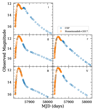
Figure 11: Comparison between the CSP photometry (blue circles) and that of Hosseinzadeh et al. (2017b) (orange circles). No S-corrections were applied to either dataset.

Table 5 lists the photometry of SN 2013aa and SN 2017cbv. Tables 6 and 7 list the photometry of the reference stars in the standard optical (Landolt, 1992; Smith et al., 2002) and NIR (Persson et al., 1998) systems. Note that there are many stars in common between the two SNe, but they were observed with different CCDs and therefore have slightly different color terms (see table 5 of Phillips et al. (2019)), yielding different standard photometry. The filter functions and photometric zero-points $zp_{\lambda}$ of the CSP-I and CSP-II natural systems are available at the CSP website. These can be used to S-correct (Stritzinger et al., 2002) the photometry to other systems. Figure 11 shows a comparison of the CSP photometry with that of Sand et al. (2018), showing very good agreement.

Appendix B Bayesian Hierarchical model for Intrinsic Dispersion

Table 8: Statistical Comparison between Surveys.

Surveys	$\left<\Delta\mu\right>$	$\sigma(sys)$	$\sigma(s_{BV})$	$\sigma(E(B-V))$	$\rho(\mu,s_{BV})$	$\rho(\mu,E(B-V))$	N
CSP/LOSS	$-0.05(03)$	$0.16$	$0.07$	$0.06$	$0.75$	$-0.69$	32
CSP/Swift	$-0.02(06)$	$0.19$	$0.07$	$0.06$	$0.31$	$-0.69$	11
CSP/CfA	$-0.03(01)$	$0.09$	$0.07$	$0.07$	$0.35$	$-0.67$	61
LOSS/Swift	$-0.07(03)$	$0.21$	$0.10$	$0.09$	$0.48$	$-0.76$	26
LOSS/CfA	$0.06(02)$	$0.16$	$0.10$	$0.08$	$0.50$	$-0.71$	87
CFA/Swift	$-0.07(04)$	$0.15$	$0.07$	$0.08$	$0.56$	$-0.93$	19

In order to quantify the intrinsic dispersion in the distances to sibling host galaxies, we construct a simple Bayesian model. For each pair of siblings, we have the difference in the distance estimate $\Delta\mu_{i,j}$ and an associated error $\sigma(\mu_{i,j})$ which we assume to be given by:

$$\sigma(\mu_{i,j})=\sqrt{\sigma(\mu_{i})^{2}+\sigma(\mu_{j})^{2}+\sigma(sys)_{i,j}^{2}},$$ (B1)

where $\sigma(\mu_{i})$ and $\sigma(\mu_{j})$ are the formal errors in the distances, including photometric uncertainties and errors in the calibration parameters (Phillips relation, extinction, etc). We also add additional systematic errors $\sigma(sys)_{i,j}$ when comparing distances using different photometric systems. These were estimated by fitting SNe Ia that were observed by two or more surveys and computing the standard deviation of the differences in distance estimates. We summarize these in Table 8. We also include the mean difference in distance $\left<\Delta\mu\right>$, the standard deviation in the light-curve parameters ($s_{BV}$ and $E(B-V)$), the Pearson correlation coefficients, and the number of SNe Ia used. The mean offsets were not applied to the distances in table 3 nor in the analysis to follow, but rather are kept as part of the error in $\sigma(sys)$. Generally speaking, the difference in distance estimates are most strongly correlated with differences in estimates in the extinction.

We model the true distribution of $\Delta\mu_{i,j}^{T}$ as a normal distribution centered at zero with scale $\sigma_{SN}$. The observed $\Delta\mu_{i,j}$ are modeled as normal distributions centered at $\Delta\mu_{i,j}^{T}$ with scale $\sigma(\mu_{i,j})$. Symbolically:

$$\sigma_{SN} \sim U(0,\infty)$$ (B2)

$$\Delta\mu_{i,J}^{T} \sim N\left(0,\sigma_{SN}\right)$$

$$\Delta\mu_{i,j} \sim N\left(\Delta\mu_{i,j}^{T},\sigma(\mu_{i,j})\right).$$

We fit for the value of $\sigma_{SN}$ using Markov Chain Monte Carlo (MCMC) methods. Table 4 lists the results with different subsets of the sibling SNe.

References

- Ashall et al. (2016) Ashall, C., Mazzali, P., Sasdelli, M., & Prentice, S. J. 2016, MNRAS, 460, 3529
- Ashall et al. (2018) Ashall, C., Mazzali, P. A., Stritzinger, M. D., et al. 2018, MNRAS, 477, 153
- Ashall et al. (2019a) Ashall, C., Hsiao, E. Y., Hoeflich, P., et al. 2019a, ApJ, 875, L14
- Ashall et al. (2019b) Ashall, C., Hoeflich, P., Hsiao, E. Y., et al. 2019b, ApJ, 878, 86
- Avelino et al. (2019) Avelino, A., Friedman, A. S., Mandel, K. S., et al. 2019, ApJ, 887, 106
- Bernstein et al. (2003) Bernstein, R., Shectman, S. A., Gunnels, S. M., Mochnacki, S., & Athey, A. E. 2003, Society of Photo-Optical Instrumentation Engineers (SPIE) Conference Series, Vol. 4841, MIKE: A Double Echelle Spectrograph for the Magellan Telescopes at Las Campanas Observatory, ed. M. Iye & A. F. M. Moorwood, 1694–1704
- Betoule et al. (2014) Betoule, M., Kessler, R., Guy, J., et al. 2014, A&A, 568, A22
- Blondin et al. (2012) Blondin, S., Matheson, T., Kirshner, R. P., et al. 2012, AJ, 143, 126
- Branch et al. (2006) Branch, D., Dang, L. C., Hall, N., et al. 2006, Publications of the Astronomical Society of the Pacific, 118, 560. https://doi.org/10.1086%2F502778
- Brown (2015) Brown, P. J. 2015, arXiv e-prints, arXiv:1505.01368
- Brown et al. (2014) Brown, P. J., Breeveld, A. A., Holland, S., Kuin, P., & Pritchard, T. 2014, Ap&SS, 354, 89
- Brown & Crumpler (2019) Brown, P. J., & Crumpler, N. R. 2019, arXiv e-prints, arXiv:1909.05445
- Brown et al. (2017) Brown, P. J., Landez, N. J., Milne, P. A., & Stritzinger, M. D. 2017, ApJ, 836, 232
- Brown et al. (2009) Brown, P. J., Holland, S. T., Immler, S., et al. 2009, AJ, 137, 4517
- Brown et al. (2010) Brown, P. J., Roming, P. W. A., Milne, P., et al. 2010, ApJ, 721, 1608
- Brown et al. (2019) Brown, P. J., Hosseinzadeh, G., Jha, S. W., et al. 2019, ApJ, 877, 152
- Burns et al. (2011) Burns, C. R., Stritzinger, M., Phillips, M. M., et al. 2011, AJ, 141, 19
- Burns et al. (2014) —. 2014, ApJ, 789, 32
- Burns et al. (2018) Burns, C. R., Parent, E., Phillips, M. M., et al. 2018, ApJ, 869, 56
- Childress et al. (2014) Childress, M. J., Vogt, F. P. A., Nielsen, J., & Sharp, R. G. 2014, Ap&SS, 349, 617
- Contreras et al. (2010) Contreras, C., Hamuy, M., Phillips, M. M., et al. 2010, The Astronomical Journal, 139, 519
- Coulter et al. (2017) Coulter, D. A., Foley, R. J., Kilpatrick, C. D., et al. 2017, Science, 358, 1556
- Dopita et al. (2007) Dopita, M., Hart, J., McGregor, P., et al. 2007, Ap&SS, 310, 255
- Elias-Rosa et al. (2008) Elias-Rosa, N., Benetti, S., Turatto, M., et al. 2008, MNRAS, 384, 107
- Fakhouri et al. (2015) Fakhouri, H. K., Boone, K., Aldering, G., et al. 2015, ApJ, 815, 58
- Fitzpatrick (1999) Fitzpatrick, E. L. 1999, PASP, 111, 63
- Folatelli et al. (2010) Folatelli, G., Phillips, M. M., Burns, C. R., et al. 2010, AJ, 139, 120
- Foley et al. (2018a) Foley, R. J., Hoffmann, S. L., Macri, L. M., et al. 2018a, arXiv e-prints, arXiv:1806.08359
- Foley et al. (2008) Foley, R. J., Filippenko, A. V., Aguilera, C., et al. 2008, ApJ, 684, 68
- Foley et al. (2018b) Foley, R. J., Scolnic, D., Rest, A., et al. 2018b, MNRAS, 475, 193
- Freedman et al. (2009) Freedman, W. L., Burns, C. R., Phillips, M. M., et al. 2009, ApJ, 704, 1036
- Friedman et al. (2015) Friedman, A. S., Wood-Vasey, W. M., Marion, G. H., et al. 2015, ApJS, 220, 9
- Galbany et al. (2018) Galbany, L., Anderson, J. P., Sánchez, S. F., et al. 2018, ApJ, 855, 107
- Gall et al. (2018) Gall, C., Stritzinger, M. D., Ashall, C., et al. 2018, A&A, 611, A58
- Garavini et al. (2007) Garavini, G., Folatelli, G., Nobili, S., et al. 2007, A&A, 470, 411
- Graham et al. (2017) Graham, M. L., Kumar, S., Hosseinzadeh, G., et al. 2017, MNRAS, 472, 3437
- Guy et al. (2007) Guy, J., Astier, P., Baumont, S., et al. 2007, A&A, 466, 11
- Hamuy et al. (1991) Hamuy, M., Phillips, M. M., Maza, J., et al. 1991, AJ, 102, 208
- Hamuy et al. (1996) Hamuy, M., Phillips, M. M., Suntzeff, N. B., et al. 1996, AJ, 112, 2391
- Hamuy et al. (2006) Hamuy, M., Folatelli, G., Morrell, N. I., et al. 2006, PASP, 118, 2
- Hicken et al. (2009) Hicken, M., Wood-Vasey, W. M., Blondin, S., et al. 2009, ApJ, 700, 1097
- Hicken et al. (2012) Hicken, M., Challis, P., Kirshner, R. P., et al. 2012, ApJS, 200, 12
- Hoeflich & Khokhlov (1996) Hoeflich, P., & Khokhlov, A. 1996, ApJ, 457, 500
- Hoeflich et al. (2017) Hoeflich, P., Hsiao, E. Y., Ashall, C., et al. 2017, ApJ, 846, 58
- Hosseinzadeh et al. (2017a) Hosseinzadeh, G., Sand, D. J., Valenti, S., et al. 2017a, ApJ, 845, L11
- Hosseinzadeh et al. (2017b) —. 2017b, ApJ, 845, L11
- Hsiao et al. (2013) Hsiao, E. Y., Marion, G. H., Phillips, M. M., et al. 2013, ApJ, 766, 72
- Hsiao et al. (2015) Hsiao, E. Y., Burns, C. R., Contreras, C., et al. 2015, A&A, 578, A9
- Hsiao et al. (2019) Hsiao, E. Y., Phillips, M. M., Marion, G. H., et al. 2019, PASP, 131, 014002
- Hunter (2007) Hunter, J. D. 2007, Computing in Science & Engineering, 9, 90
- Jha et al. (2007) Jha, S., Riess, A. G., & Kirshner, R. P. 2007, ApJ, 659, 122
- Jha et al. (2006) Jha, S., Kirshner, R. P., Challis, P., et al. 2006, AJ, 131, 527
- Jones et al. (2018) Jones, D. O., Scolnic, D. M., Riess, A. G., et al. 2018, ApJ, 857, 51
- Kattner et al. (2012) Kattner, S., Leonard, D. C., Burns, C. R., et al. 2012, PASP, 124, 114
- Kelly et al. (2010) Kelly, P. L., Hicken, M., Burke, D. L., Mandel, K. S., & Kirshner, R. P. 2010, ApJ, 715, 743
- Kelson (2003) Kelson, D. D. 2003, PASP, 115, 688
- Koribalski et al. (2004) Koribalski, B. S., Staveley-Smith, L., Kilborn, V. A., et al. 2004, AJ, 128, 16
- Krisciunas et al. (2000) Krisciunas, K., Hastings, N. C., Loomis, K., et al. 2000, ApJ, 539, 658
- Krisciunas et al. (2004) Krisciunas, K., Phillips, M. M., & Suntzeff, N. B. 2004, ApJ, 602, L81
- Krisciunas et al. (2017) Krisciunas, K., Contreras, C., Burns, C. R., et al. 2017, AJ, 154, 211
- Lampeitl et al. (2010) Lampeitl, H., Smith, M., Nichol, R. C., et al. 2010, ApJ, 722, 566
- Landolt (1992) Landolt, A. U. 1992, AJ, 104, 340
- Livio & Mazzali (2018) Livio, M., & Mazzali, P. 2018, Phys. Rep., 736, 1
- Livne & Arnett (1995) Livne, E., & Arnett, D. 1995, ApJ, 452, 62
- Mandel et al. (2009) Mandel, K. S., Wood-Vasey, W. M., Friedman, A. S., & Kirshner, R. P. 2009, ApJ, 704, 629
- Marion et al. (2016) Marion, G. H., Brown, P. J., Vinkó, J., et al. 2016, ApJ, 820, 92
- Milne et al. (2013) Milne, P. A., Brown, P. J., Roming, P. W. A., Bufano, F., & Gehrels, N. 2013, ApJ, 779, 23
- Oke & Sandage (1968) Oke, J. B., & Sandage, A. 1968, ApJ, 154, 21
- Pan et al. (2019) Pan, Y. C., Foley, R. J., Jones, D. O., Filippenko, A. V., & Kuin, N. P. M. 2019, arXiv e-prints, arXiv:1906.09554
- Pastorello et al. (2007) Pastorello, A., Mazzali, P. A., Pignata, G., et al. 2007, MNRAS, 377, 1531
- Persson et al. (2004) Persson, S. E., Madore, B. F., Krzemiński, W., et al. 2004, The Astronomical Journal, 128, 2239
- Persson et al. (1998) Persson, S. E., Murphy, D. C., Krzeminski, W., Roth, M., & Rieke, M. J. 1998, AJ, 116, 2475
- Phillips (1993) Phillips, M. M. 1993, ApJ, 413, L105
- Phillips et al. (1999) Phillips, M. M., Lira, P., Suntzeff, N. B., et al. 1999, AJ, 118, 1766
- Phillips et al. (1992) Phillips, M. M., Wells, L. A., Suntzeff, N. B., et al. 1992, AJ, 103, 1632
- Phillips et al. (2013) Phillips, M. M., Simon, J. D., Morrell, N., et al. 2013, ApJ, 779, 38
- Phillips et al. (2019) Phillips, M. M., Contreras, C., Hsiao, E. Y., et al. 2019, PASP, 131, 014001
- Poznanski et al. (2012) Poznanski, D., Prochaska, J. X., & Bloom, J. S. 2012, MNRAS, 426, 1465
- Pskovskii (1984) Pskovskii, Y. P. 1984, Soviet Ast., 28, 658
- Riess et al. (1996) Riess, A. G., Press, W. H., & Kirshner, R. P. 1996, ApJ, 473, 88
- Riess et al. (1999) Riess, A. G., Kirshner, R. P., Schmidt, B. P., et al. 1999, AJ, 117, 707
- Sand et al. (2018) Sand, D. J., Graham, M. L., Botyánszki, J., et al. 2018, ApJ, 863, 24
- Schlafly & Finkbeiner (2011) Schlafly, E. F., & Finkbeiner, D. P. 2011, ApJ, 737, 103
- Scolnic et al. (2020) Scolnic, D., Smith, M., Massiah, A., et al. 2020, arXiv e-prints, arXiv:2002.00974
- Shen et al. (2018) Shen, K. J., Kasen, D., Miles, B. J., & Townsley, D. M. 2018, ApJ, 854, 52
- Shen & Moore (2014) Shen, K. J., & Moore, K. 2014, ApJ, 797, 46
- Silverman et al. (2012) Silverman, J. M., Foley, R. J., Filippenko, A. V., et al. 2012, MNRAS, 425, 1789
- Simon et al. (2010) Simon, J. D., Frebel, A., McWilliam, A., Kirby, E. N., & Thompson, I. B. 2010, ApJ, 716, 446
- Smith et al. (2002) Smith, J. A., Tucker, D. L., Kent, S., et al. 2002, AJ, 123, 2121
- Stritzinger et al. (2005) Stritzinger, M., Suntzeff, N. B., Hamuy, M., et al. 2005, PASP, 117, 810
- Stritzinger et al. (2002) Stritzinger, M., Hamuy, M., Suntzeff, N. B., et al. 2002, AJ, 124, 2100
- Stritzinger et al. (2010) Stritzinger, M., Burns, C. R., Phillips, M. M., et al. 2010, The Astronomical Journal, 140, 2036
- Stritzinger et al. (2011) Stritzinger, M. D., Phillips, M. M., Boldt, L. N., et al. 2011, AJ, 142, 156
- Sullivan et al. (2010) Sullivan, M., Conley, A., Howell, D. A., et al. 2010, MNRAS, 755
- The Astropy Collaboration et al. (2018) The Astropy Collaboration, Price-Whelan, A. M., Sipőcz, B. M., et al. 2018, AJ, 156, 123
- Walker et al. (2012) Walker, E. S., Hachinger, S., Mazzali, P. A., et al. 2012, MNRAS, 427, 103
- Wang et al. (2013) Wang, X., Wang, L., Filippenko, A. V., Zhang, T., & Zhao, X. 2013, Science, 340, 170
- Wee et al. (2018) Wee, J., Chakraborty, N., Wang, J., & Penprase, B. E. 2018, ApJ, 863, 90
- Wheeler et al. (1998) Wheeler, J. C., Höflich, P., Harkness, R. P., & Spyromilio, J. 1998, ApJ, 496, 908
- Wood-Vasey et al. (2008) Wood-Vasey, W. M., Friedman, A. S., Bloom, J. S., et al. 2008, ApJ, 689, 377
- Yaron & Gal-Yam (2012) Yaron, O., & Gal-Yam, A. 2012, PASP, 124, 668