On infinite staircases in toric symplectic four-manifolds

Abstract.

An influential result of McDuff and Schlenk asserts that the function that encodes when a four-dimensional symplectic ellipsoid can be embedded into a four-dimensional ball has a remarkable structure: the function has infinitely many corners, determined by the odd-index Fibonacci numbers, that fit together to form an infinite staircase.

This work has recently led to considerable interest in understanding when the ellipsoid embedding function for other symplectic $4$-manifolds is partly described by an infinite staircase. We provide a general framework for analyzing this question for a large family of targets, called finite type convex toric domains, which we prove generalizes the class of closed toric symplectic four-manifolds. When the target is of finite type, we prove that any infinite staircase must have a unique accumulation point $a_{0}$, given as the solution to an explicit quadratic equation. Moreover, we prove that the embedding function at $a_{0}$ must be equal to the classical volume lower bound. In particular, our result gives an obstruction to the existence of infinite staircases that experimentally seems strong. Our methods apply equally well to any closed manifold which is a blow-up of the complex projective plane.

In the special case of rational convex toric domains, we can say more. We conjecture a complete answer to the question of existence of infinite staircases, in terms of six families that are distinguished by the fact that their moment polygon is reflexive. We then provide a uniform proof of the existence of infinite staircases for our six families, using two tools. For the first, we use recursive families of almost toric fibrations to find symplectic embeddings into closed symplectic manifolds. In order to establish the embeddings for convex toric domains, we prove a result of potentially independent interest: a four-dimensional ellipsoid embeds into a closed toric symplectic four-manifold if and only if it can be embedded into a corresponding convex toric domain. For the second tool, we find recursive families of convex lattice paths that provide obstructions to embeddings. We conclude by connecting our conjecture that these are the only infinite staircases among rational convex toric domains to a question in number theory related to a classic work of Hardy and Littlewood.

1. Introduction

In the past two decades, there has been considerable interest in and progress on the question of whether there is an embedding

$$(M,\omega_{M}){\stackrel{{\scriptstyle s}}{{\hookrightarrow}}}(N,\omega_{N})$$

preserving symplectic structures, or whether the existence of such a map is in some way obstructed. On the one hand, Local Normal Form theorems and clever constructions like symplectic folding and symplectic inflation allow us to find embeddings. On the other hand, there are well-developed tools involving pseudo-holomorphic curves that provide numerous obstructions to these maps.

A landmark result about this is the celebrated work of McDuff and Schlenk, who completely determined when a four-dimensional ellipsoid

$$E(a,b)=\left\{(z_{1},z_{2})\in\mathbb{C}^{2}:\pi\left(\frac{|z_{1}|^{2}}{a}+\frac{|z_{2}|^{2}}{b}\right)<1\right\}$$

can be symplectically embedded into a four-dimensional ball $B(a)=E(a,a)$. They found that when the ellipsoid is close to round, the answer is extremely delicate, determined by the odd-index Fibonacci numbers and the Golden Mean. On the other hand, if the ellipsoid is sufficiently stretched then the only obstruction to an embedding is the classical volume obstruction.

Since the work of McDuff and Schlenk, many examples of infinite staircases have been found; we will survey what is known below. There is moreover an extensive literature on symplectic embedding problems where the domain is an ellipsoid: [7, 8, 10, 11, 12, 13, 16, 21, 27, 28, 30, 31, 46, 47, 48, 50, 52, 53, 59]. However, a general theory of infinite staircases does not currently exist. We do not know how characteristic infinite staircases are for symplectic embedding problems. For any fixed target, we do not know how to determine if there is an infinite staircase. We also do not know if all examples of this phenomenon can be unified in an elegant way or whether their corresponding symplectic embeddings share common features. There are other mysteries: for instance, in every target known to admit an infinite staircase, the stairs alternate between being horizontal and being linear with no constant term.

Our interest here is in taking some useful first steps towards better understanding these questions.

To fix notation, let $X$ be a symplectic $4$-manifold. We write $E{\stackrel{{\scriptstyle s}}{{\hookrightarrow}}}X$ to mean that there is a symplectic embedding of $E$ into $X$, and define the ellipsoid embedding function of $X$ by

(1.1) $$c_{X}(a):=\inf\left\{\lambda\ \big{|}\ E(1,a){\stackrel{{\scriptstyle s}}{{\hookrightarrow}}}\lambda X\right\},\mbox{ for }a\geq 1,$$

where $\lambda X$ represents the symplectic scaling $(X,\lambda\cdot\omega)$ of $(X,\omega)$. We could have defined the function for $a>0$, but there is a symmetry across $a=1$, making this redundant. This is a nondecreasing function; it is also continuous, although we will not prove that in full generality here. Inspired by the McDuff-Schlenk result, we make the following definition.

Definition 1.2.

We say that the ellipsoid embedding function $c_{X}(a)$ has an infinite staircase if its graph has infinitely many non-smooth points on some compact interval, i.e. infinitely many staircase steps.

For a general $X$ with no further assumptions, computing the function $c_{X}(a)$ exactly or even determining whether or not it has an infinite staircase is presumably impossible due to the subtle mix of obstructions and constructions alluded to above. For example, when $X$ is star-shaped domain, it is known that the periods of certain Reeb orbits on the boundary give obstructions to the existence of an embedding. Moreover one has the impression that a certain amount of additional structure on $X$ is required for an infinite staircase to exist. So, one should make some restrictions on $X$. The starting point for our investigations is the following question. Let $X$ be a closed toric symplectic four-manifold associated to a moment polygon $\Omega$ in $\mathbb{R}^{2}$; this is a rich source of interesting examples. Can we determine from $\Omega$ whether or not $c_{X}$ has an infinite staircase? The answers we have found are governed by beautiful combinatorics and number theory.

In fact, most of our results should hold for more general closed four-manifolds $X$, for example rational $X$ or Hamiltonian $S^{1}$-manifolds, or even uniruled $X$, see §1.3, but that is not our focus here.

To state our results, we now introduce the related notion of toric domains. A 4-dimensional toric domain $X$ is the preimage of a domain $\Omega\subset\mathbb{R}_{\geq 0}^{2}$ under the moment map

$$\mu:\mathbb{C}^{2}\to\mathbb{R}^{2},\qquad(z_{1},z_{2})\mapsto(\pi|z_{1}|^{2},\pi|z_{2}|^{2}).$$

For example, if $\Omega$ is the hypotenuse-less triangle with vertices $(0,0)$, $(a,0)$, and $(0,b)$, then $X_{\Omega}$ is the open ellipsoid $E(a,b)$. Following the notation set forth in [9, Definition 1.1], a convex toric domain is the preimage under $\mu$ of a closed region $\Omega\subset\mathbb{R}_{\geq 0}^{2}$ that is convex, connected, and contains the origin in its interior. We denote this $X_{\Omega}=\mu^{-1}(\Omega)$ and call the region $\Omega$ the moment polygon of $X_{\Omega},$ in analogy with the case of closed toric symplectic manifolds.

One motivation for studying convex toric domains comes from the following result that we prove, which ties together the ellipsoid embedding functions for closed toric manifolds and convex toric domains. This result features essentially in our proof of Theorem 1.16 as well.

Theorem 1.3.

Let $\Omega\subset\mathbb{R}_{\geq 0}^{2}$ be a convex region that is also a Delzant polygon for a closed toric symplectic four-manifold $M$. Then there exists a symplectic embedding

(1.4) $$E(d,e){\stackrel{{\scriptstyle s}}{{\hookrightarrow}}}M$$

if and only if there exists a symplectic embedding

(1.5) $$E(d,e){\stackrel{{\scriptstyle s}}{{\hookrightarrow}}}X_{\Omega}.$$

Thus, from the point of view of the function $c_{X}$, convex toric domains significantly generalize closed toric manifolds. In fact, we can relate embeddings into convex toric domains to embeddings into closed manifolds in a slightly more general context, including some well-known examples, for example equilateral pentagon space: see Remark 3.3, Proposition 3.5, and the accompanying Remark 3.6.

For a general convex toric domain $X$, the embedding function $c_{X}(a)$ has an interesting qualitative structure. For a fixed $X$, the volume curve is the curve $y=\sqrt{\frac{a}{\text{vol}}}$ and the constraint

$$c_{X}(a)\geq\sqrt{\frac{a}{\text{vol}}}$$

holds because

$$E(1,a){\stackrel{{\scriptstyle s}}{{\hookrightarrow}}}\lambda X\Rightarrow\text{volume}(E(1,a))\leq\text{volume}(\lambda X)\Leftrightarrow a\leq\lambda^{2}\text{volume}(X)\Leftrightarrow\lambda\geq\sqrt{\frac{a}{\text{vol}}}.$$

We will show in Proposition 2.1 that $c_{X}(a)$ is continuous and non-decreasing, but not generally $C^{1}$. For sufficiently large $a$, we also show that the function $c_{X}(a)$ remains equal to the volume curve: this is the phenomenon known as packing stability. Moreover, the function $c_{X}(a)$ is piecewise linear when not equal to the volume curve, except at points that are limit points of singular points of $c_{X}$. We call these limit points accumulation points and they are an important focus of this paper.

Remark 1.6.

In [7, Definition 1.1], Casals and Vianna work with a different concept, a sharp infinite staircase. This is an infinite staircase where infinitely many of the non-smooth points must be on the volume curve. That notion therefore excludes the $J=3$ cases below (cf. Remark 1.19 and Figure 1.14(b)).

All known examples of infinite staircases are associated to convex toric domains and we now survey what is known. In the paper [16], Cristofaro-Gardiner and Kleinman studied the ellipsoid embedding function of an ellipsoid $c_{E(1,b)}(a)$ and found infinite staircases when $b=2$ and $b=\frac{3}{2}$. Frenkel and Müller found an infinite staircase in the ellipsoid embedding function for a polydisc $P(1,1)$ [21], where the function is governed by the Pell numbers. Cristofaro-Gardiner, Frenkel, and Schlenk have shown that the only infinite staircase in the ellipsoid embedding function for polydisks $P(1,b)$ with $b\in\mathbb{N}$ is when $b=1$ [11]. By contrast, Usher studied ellipsoid embedding functions for irrational polydisks $P(1,b)$ [59] and found the first infinite families of infinite staircases. Usher’s families all have $b$ quadratic irrationalities of a special form.

Further work, in part making use of our Theorem 1.11 below, by Bertozzi, Holm, Maw, Mwakyoma, McDuff, Pires, and Weiler [3], Magill and McDuff [41], and Magill, McDuff and Weiler [42] studies ellipsoid embedding functions for one point blowups of $\mathbb{C}P^{2}$, varying the symplectic size of the blowup. Like Usher, they identify infinite families of infinite staircases; they also find infinitely many intervals of blowup size where an infinite staircase cannot exist. We will say a little more about their work at the end of Section 1.2 below.

1.1. Accumulation points of infinite staircases

Our first main result is aimed at rooting out the “germs” of infinite staircases. If the function $c_{X}(a)$ has an infinite staircase, then the singular points must accumulate at some set of points, otherwise this would contradict packing stability. We show that if an infinite staircase exists, there is in fact a unique such accumulation point; moreover, it can be characterized as the solution to an explicit quadratic equation determined by $\Omega$.

We now make this precise, following [9, §2.2]. To a convex toric domain $X_{\Omega}$ we can associate a negative weight expansion $(b;b_{1},b_{2},\ldots)$. To do so, first we need to define a $b$-triangle to be the triangle with vertices $(0,0)$, $(b,0)$ and $(0,b)$ or any $AGL(2,\mathbb{Z})$ transformation of it. We proceed inductively: let $b$ be the smallest number such that $\Omega$ is contained in a $b$-triangle. If $\Omega$ equals that triangle, we are done. Otherwise, let $b_{1}>0$ be the largest value such that $\Omega$ is contained in the original $b$-triangle minus a $b_{1}$-triangle that is removed at a corner of the $b$-triangle. If $\Omega$ equals this quadrilateral, we are done. Otherwise, let $b_{2}>0$ be the largest value such that $\Omega$ is contained in the previous quadrilateral minus a $b_{2}$-triangle that is removed at one of its corners. The removing of the $b_{i}$-triangles is reminiscent of what is done to the moment polytope when performing equivariant symplectic blowups at fixed points. We note that when $\Omega$ is a lattice polygon, this procedure is finite.

We note that two different convex toric domains can have the same negative weight expansion, see Figure 1.8 for examples. We will see in Remark 2.8 that the relevant feature of a convex toric domain in the context of this paper is its negative weight expansion, and not the actual shape of $\Omega$.

Definition 1.7.

We say that a negative weight expansion $(b;b_{1},b_{2},\ldots)$ is finite if there are finitely many non-zero $b_{i}$’s, and we say that such a convex toric domain $X_{\Omega}$ has finite type. Given a finite type convex toric domain $X$ with negative weight expansion $(b;b_{1},\ldots,b_{n})$, we define:

$$\begin{split}\text{per}&=3b-\sum_{i=1}^{n}b_{i}\\ \text{vol}&=b^{2}-\sum_{i=1}^{n}b_{i}^{2}.\end{split}$$

We say that $X_{\Omega}$ is a rational convex toric domain if $b,b_{1},\ldots,b_{n}$ are all rational numbers.

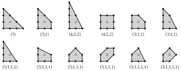
Figure 1.8. Regions corresponding to finite type rational convex toric domains, and their negative weight expansions $(b;b_{1},\ldots,b_{n})$. The negative weight expansions $(3;1)$ and $(3;1,1)$ correspond to the $J=3$ case and all others are $J=2$; cf. Table 1.15 and Remark 1.19. Note that all of these polygons are reflexive: each is a lattice polygon with precisely one interior lattice point.

Remark 1.9.

Finite type convex toric domains generalize closed toric symplectic four-manifolds as targets for ellipsoid embedding functions in the following sense. Theorem 1.3 makes a correspondence between closed toric symplectic manifolds and convex toric domains that have the same moment image in $\mathbb{R}^{2}$. The proof of Theorem 1.3 explains why the convex toric domains that arise in this way are always of finite type, while Remark 3.3 discusses an example of a finite type convex toric domain that does not arise from a closed toric symplectic four-manifold.

We note that all convex toric domains in Theorem 1.16 are rational. The significance of this property is also highlighted by Conjecture 1.20.

Remark 1.10.

The quantities per and vol are, respectively, the affine perimeter and twice the area of the region in $\mathbb{R}^{2}$ representing $X$. They are well-defined as invariants of $X$. In particular, vol is the symplectic volume of $X$. Note also that $\frac{\text{per}^{2}}{\text{vol}}$ is invariant under scaling of (the region representing) $X$.

We can now state precisely our theorem about finding accumulation points.

Theorem 1.11.

Let $X$ be a finite type convex toric domain. If the ellipsoid embedding function $c_{X}(a)$ has an infinite staircase then it accumulates at $a_{0}$, a real solution of the quadratic equation

(1.12) $$a^{2}-\left(\frac{\text{per}^{2}}{\text{vol}}-2\right)a+1=0.$$

Furthermore, at $a_{0}$ the ellipsoid embedding function touches the volume curve:

$$c_{X}(a_{0})=\sqrt{\frac{a_{0}}{\text{vol}}}\phantom{..}.$$

We emphasize that, for any particular finite type target $X_{\Omega}$, Theorem 1.11 leads to the following procedure for approaching the question of whether or not $X_{\Omega}$ has an infinite staircase. We compute the quantity $c_{X_{\Omega}}(a_{0})-\sqrt{\frac{a_{0}}{\text{vol}}}\geq 0$, which we call the staircase obstruction. If the staircase obstruction is positive, then there cannot be an infinite staircase. For example, the staircase obstruction is positive in Figure 1.14(c) below, where we can see clearly that the ellipsoid embedding function is obstructed at $a_{0}$, and so a toric domain with negative weight expansion $(4;2,1)$ cannot have an infinite staircase. The staircase obstruction seems to give a strong indication about the possibility of an infinite staircase. In our experience, it is almost always sharp.

If the staircase obstruction vanishes, then by Theorem 1.11, if there is an infinite staircase, it still must exist in a neighborhood of $a_{0}$. In this case, one can attempt to explore the question numerically, near $a_{0}$, using for example the combinatorial formulas in [9, Thm. A.1, Cor. A.12 ], to see whether or not the existence of an infinite staircase is likely. In fact, there are only a handful of known examples where the staircase obstruction vanishes but there is no staircase. One such is shown in Figure 1.14(d). The negative weight expansion $(4,1,1,1,1)$ corresponds to $X_{\Omega}=E(3,4)$. Cristofaro-Gardiner has computed the ellipsoid embedding function on a neighborhood of $a_{0}$ and proved that it does not have an infinite staircase [10, Sec. 2.5]. In all known examples, a procedure analogous to this one is decisive.

Theorem 1.11 can also be used to rule out the existence of infinite staircases for families of targets. For example, in [3], Theorem 1.11 is used to identify intervals of $b$ for which the ellipsoid embedding function of a toric domain with negative weight expansion $(1;b)$ cannot have an infinite staircase. Theorem 1.11 is also useful for finding infinite staircases, as we explain in Appendix C. In [10], it is used to completely determine which rational ellipsoids have infinite staircases.

Remark 1.13.

Theorem 1.11 has an interesting interpretation in terms of the asymptotics of ECH capacities. We review the theory of ECH capacities in Section 2.2. Theorem 1.11 can be interpreted as saying that at an accumulation point of singular points, the leading and subleading asymptotics of the ECH capacities of the domain and target agree. For more about this, see Remark 4.10.

It might also be interesting to note that in the case of a rational convex toric domain, the coefficients of (1.12) are rational. In particular, $a_{0}$ is a quadratic surd for these examples. This is potentially useful for ruling out infinite staircases, as we further explore in Section 6.

1.2. Reflexive polygons and infinite staircases

Having explained in the previous section where infinite staircases must accumulate, we now turn our attention to finding and describing them. We begin by showing in Figure 1.14 the types of graphs we can produce of embedding functions using Mathematica. These types of plots, analyzed via Theorem 1.16, were essential in our early investigations of infinite staircases. This is discussed further in Appendix C.

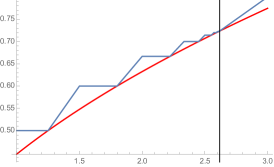
(a) $(3;1,1,1,1)$

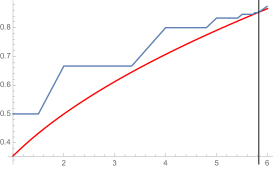
(b) $(3;1)$

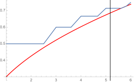
(c) $(4;2,1)$

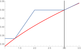
(d) $(4;1,1,1,1)$

Figure 1.14. Plots of ellipsoid embedding functions for different domains, labeled by their negative weight expansion. The red curves are the volume curves and the vertical lines indicate where the accumulation points would necessarily be located, if a staircase existed, per Theorem 1.11. The top two plots have infinite staircases: in (a) we have a $J=2$ case, where the inner corners touch the volume curve (a sharp infinite staircase); and in (b) we have a $J=3$ case, where the inner corners approach but do not touch the volume curve. The plots (c) and (d) do not have infinite staircases: (c) has non-zero staircase obstruction, while showing that (d) does not have a staircase is intricate [10].

Our next result identifies infinite staircases for the ellipsoid embedding functions of twelve convex toric domains, including the already known ball, polydisk $P(1,1)$, and $E(1,\frac{3}{2})$. Our proof of Theorem 1.16 provides a uniform approach to prove the existence of all twelve in one fell swoop. The graphs of these functions are related to certain recurrence sequences, which are given in Table 1.15. We remark that the scale invariant quantity $\frac{\text{per}^{2}}{\text{vol}}$, together with the length of recurrence, determines the recurrence relation.

Negative weight expansion	Recurrence relation	Seeds	$K=\frac{\text{per}^{2}}{\text{vol}}-2$	$J$	$a_{0}$
	$g(n+2J)=Kg(n+J)-g(n)$	$g(0),\ldots,g(2J-1)$
$(3)$	$g(n+4)=7g(n+2)-g(n)$	$2,1,1,2$	7	2	$\frac{7+3\sqrt{5}}{2}$
$(4;2,2)$	$g(n+4)=6g(n+2)-g(n)$	$1,1,1,3$	6	2	$3+2\sqrt{2}$
$(3;1,1,1)$	$g(n+4)=4g(n+2)-g(n)$	$1,1,1,2$	4	2	$2+\sqrt{3}$
$(3;1,1,1,1)$	$g(n+4)=3g(n+2)-g(n)$	$1,2,1,3$	3	2	$\frac{3+\sqrt{5}}{2}$
$(3;1)$	$g(n+6)=6g(n+3)-g(n)$	$1,1,1,1,2,4$	6	3	$3+2\sqrt{2}$
$(3;1,1)$	$g(n+6)=5g(n+3)-g(n)$	$1,1,1,1,2,3$	5	3	$\frac{5+\sqrt{21}}{2}$

Table 1.15. The key recurrence relations.

Theorem 1.16.

Let $X$ be a convex toric domain with negative weight expansion $(b;b_{1},\ldots,b_{n})$ equal to

$$(3)\ ,\ (3;1)\ ,\ (3;1,1)\ ,\ (3;1,1,1)\ ,\ (3;1,1,1,1)\ ,\mbox{or }(4;2,2).$$

Then the ellipsoid embedding function $c_{X}(a)$ has an infinite staircase which alternates between horizontal lines and lines through the origin connecting inner and outer corners

$$(x^{\text{in}}_{0},y^{\text{in}}_{0}),(x^{\text{out}}_{1},y^{\text{out}}_{1}),(x^{\text{in}}_{1},y^{\text{in}}_{1}),(x^{\text{out}}_{2},y^{\text{out}}_{2}),\ldots$$

respectively with coordinates:

$$(x^{\text{in}}_{n},y^{\text{in}}_{n})=\left(\frac{g(n+J)\left(g(n+1)+g(n+1+J)\right)}{\left(g(n)+g(n+J)\right)g(n+1)},\frac{g(n+J)}{g(n)+g(n+J)}\right),$$

$$(x^{\text{out}}_{n},y^{\text{out}}_{n})=\left(\frac{g(n+J)}{g(n)},\frac{g(n+J)}{g(n)+g(n+J)}\right).$$

Remark 1.17.

The recurrence relations that appear in Table 1.15 do not immediately appear to be the ones previously associated to infinite staircases. But a quick computation shows that for $(3)$, this does recover the odd-index Fibonacci numbers McDuff and Schlenk found in [50]; for $(4;2,2)$ it recovers Pell and half-companion Pell numbers as found by Frenkel and Müller [21]; and for $(3;1,1,1)$ the sequences of Cristofaro-Gardiner and Kleinman [16]. Writing them in this uniform way simplifies the statement of Theorem 1.16.

Remark 1.18.

Combining Theorems 1.3 and 1.16, we conclude that the ellipsoid embedding function $c_{X}(a)$ has an infinite staircase for symplectic forms on the compact symplectic manifolds $\mathbb{C}P^{1}_{2}\times\mathbb{C}P^{1}_{2}$ and $\mathbb{C}P^{2}_{3}\#k\overline{\mathbb{C}P}^{2}_{1}$ for $k=0,1,2,3,4$. The smooth polygons in Figure 1.8 are Delzant polygons: they are the moment polygons of compact toric symplectic manifolds, namely with underlying smooth manifold $\mathbb{C}P^{1}\times\mathbb{C}P^{1}$ and $\mathbb{C}P^{2}\#k\overline{\mathbb{C}P}^{2}$ for $k=0,1,2,3$. The only negative weight expansion from the list that does not have a smooth Delzant polygon representative is $(3;1,1,1,1)$. This manifold is well known not to admit a Hamiltonian circle or $2$-torus action [25]. We may identify this manifold as equilateral pentagon space and as such, it is well known to admit a completely integrable system from bending flows whose image is shown in the bottom right picture in Figure 1.8.

Remark 1.19.

For each convex toric domain, the accumulation point of the infinite staircase is on the volume curve. However, two fairly distinct behaviors can be observed, related to the order of the recurrence relation in Table 1.15. In the $J=2$ cases, the inner corners of the infinite staircase are on the volume curve, whereas in the $J=3$ cases, they approach the volume curve but never touch it. Examples are shown in Figure 1.14(a) and (b). Wherever the staircase hits the volume curve, it indicates that there is a full filling of the target by the ellipsoid. The behavior when $J=3$ has not previously been observed for rational convex toric domains.

These two different behaviours can be seen explicitly in the Proof of Proposition 5.9, which following a beautiful idea of Casals and Vianna uses sequences of almost toric fibrations to construct symplectic embeddings corresponding to the inner corners of the staircase. In the $J=2$ case, the base diagrams of the almost toric fibrations are triangles, which give full filling ellipsoids. In the $J=3$ case, the base diagrams are quadrilaterals and the embeddings are determined by the biggest triangle contained in each quadrilateral, and therefore do not constitute a full filling. See also [7] and the note at the end of the introduction of this manuscript.

We complete the introduction with a conjecture that the list in Theorem 1.16 is in a suitable sense exhaustive.

Recall that a convex lattice polygon is reflexive if it has exactly one interior lattice point; this is equivalent to requiring that its dual polygon is also a lattice polygon. Up to $AGL_{2}(\mathbb{Z})$, the only domains which have negative weight expansions listed in Theorem 1.16 are the ones shown in Figure 1.8. These are well known as twelve of the sixteen reflexive lattice polygons in $\mathbb{R}^{2}$; the other four appear in Figure 6.15, and do not have infinite staircases as part of their ellipsoid embedding function.

Conjecture 1.20.

If the ellipsoid embedding function of a rational convex toric domain has an infinite staircase, then its moment polygon is a scaling of a reflexive polygon.

In particular, if Conjecture 1.20 holds, we will see that the only rational convex toric domains whose ellipsoid embedding function has an infinite staircase are indeed the ones from Theorem 1.16 or any scaling of those, by ruling out the remaining four reflexive polygons. We will use Theorem 1.11 to give some evidence supporting Conjecture 1.20 in this paper; as further evidence, Cristofaro-Gardiner’s paper [10] applies Theorem 1.11 to prove Conjecture 1.20 in the special case of ellipsoids.

In light of the recent work [3, 59] about infinite staircases for irrational targets, it is crucial in Conjecture 1.20 that the toric domain be rational. That said, it would be compelling to try to fit the examples from [3, 59] into a more general framework in the spirit of Conjecture 1.20. For some very interesting work related to this in the case of one-point blowups, we refer the reader to [3, 41, 42]; for example, as explained in [43], one part of a beautiful conjecture by the authors there is that all infinite staircases in this case are either the known rational examples (including the example from this present work) or correspond to endpoints of open intervals of blow-up size $b$ for which the staircase obstruction from Theorem 1.11 does not vanish. It also would be interesting to explore the almost toric fibration methods in this context; for example, perhaps the embeddings required in the irrational examples can also be constructed via polytope mutation; see also [41, 42, 43].

1.3. Other closed targets

We have chosen to focus our attentions here on the toric case, but the methods should work equally well for some other natural targets. For instance, recall that a closed symplectic $4$-manifold is rational if it is a product of spheres or a blow-up of $\mathbb{C}P^{2}$. The case of the product of spheres is already toric. As for a blow-up of $\mathbb{C}P^{2}$, Theorem 1.11 still holds, by essentially the same argument, where in the definition of per and vol, we use the size of the blow-ups instead of the negative weight expansion.

More generally, recall that a symplectic manifold is called uniruled if there is a nonzero genus zero Gromov-Witten invariant with a point constraint. For example, any Hamiltonian $S^{1}$-manifold is uniruled [49] as is any rationally connected manifold. By a fundamental result of McDuff [45], the only closed uniruled symplectic 4-manifolds are rational or ruled, which means that the manifold is a blow-up of an $S^{2}$ bundle over a Riemann surface. We discussed the rational case above; as for a manifold which is ruled but not rational (which is called irrationally ruled), one in fact should be able to show that infinite staircases do not ever exist. Indeed, the ball-packing problem is known to have a straightforward answer for these targets, first by the work of Biran [4, Cor. 5.C] in the case of products and then by Holm and Kessler in the general case, see [29, Lem. 4.8]; and, by a straightforward modification of the argument in [46], it should be possible to show that an ellipsoid embeds into an irrationally ruled manifold if and only if a corresponding ball-packing problem, analogous to (2.14) below, has a solution.

We should also remark that for many targets, for example linear torii, the ellipsoid embedding problem should be completely unobstructed; see [37, 19]. In fact, the embedding obstructions in our work here and in all known examples of infinite staircases are encoded in exceptional spheres, and these are most interesting in the irrational and ruled case by for example [40, Cor. 3].

Organization of the paper

We begin in Section 2 by reviewing the basic properties of ellipsoid embedding functions, ECH capacities, convex lattice paths, obstructive classes, toric manifolds, and almost toric fibrations. Next, we explore the relationship between convex toric domains and compact toric manifolds in Section 3, proving Theorem 1.3. In Section 4, we turn to the proof of Theorem 1.11. We are then able give our unified proof of the existence of the infinite staircases (Theorem 1.16) in Section 5. We conclude by describing evidence supporting our Conjecture, in Section 6, that the six examples described here are the only examples among rational convex toric domains.

The paper also includes three appendices: the first, Appendix A, draws together some combinatorial data used to define families of convex lattice paths $\Lambda_{n}$ needed to find obstructions for the proof of Theorem 1.16. The second, Appendix B, describes seeds for the families of almost toric fibrations needed to provide embeddings in the proof of Theorem 1.16. Finally, in Appendix C, we recall the very beginning of the project, including a surprise connection to the numbered stops on a Philadelphia subway line. This appendix also contains the Mathematica code we used to estimate ellipsoid embedding functions and search for infinite staircases.

Acknowledgements. We are deeply grateful for the support of the Institute for Advanced Study, without which we would not have been in the same place at the same time (with lovely lunches) to begin this project, nor continue our conjectural work during an engaging Summer Collaborators visit. We were encouraged and helped along by conversations with: Roger Casals, Helmut Hofer, Yael Karshon, Alex Kontorovich, Nicole Magill, Emily Maw, Dusa McDuff, Peter Sarnak, Felix Schlenk, Ivan Smith, Margaret Symington, Renato Vianna, and Morgan Weiler.

Joyful delays in the completion of the project were caused by the births of Amália (ARP), Hannah (TSH), and Emily (DCG).

DCG was supported by NSF grant DMS 1711976 and the Minerva Research Foundation.

TSH was supported by NSF grant DMS 1711317 and the Simons Foundation.

AM was supported by FCT/Portugal through project PTDC/MAT-PUR/29447/2017.

ARP was supported by a Simons Foundation Collaboration Grant for Mathematicians.

Relation to [7]. This article has been posted simultaneously with that of Roger Casals and Renato Vianna [7]. Their Theorem 1.2 coincides with our Proposition 5.9 for the negative weight expansions $(3)$, $(3;1,1,1)$, $(3;1,1,1,1)$, and $(4;2,2)$. Both collaborations have benefitted from our exchanges of ideas. Indeed, our initial proof relied solely on ECH capacities, but required additional technical details and guaranteed existence of an infinite staircase without completely computing the embedding capacity function.

When Pires gave a talk on this topic at a 2017 KCL/UCL Geometry Seminar, Casals shared his beautiful idea: that mutation sequences of ATFs provided explicit symplectic embeddings for the Fibonacci staircase and should do the same whenever the target region $\Omega$ is a triangle, that is, corresponding to the negative weight expansions $(3)$, $(4;2,2)$ and $(3;1,1,1)$. Following this suggestion, we were then able to implement these ATFs explicitly and uniformly for all of our target regions, including the non-triangular ones. This clarified and simplified our work and allowed us to pin down the embedding capacity function entirely, rather than just providing an existence proof for infinite staircases. Independently and without mutual knowledge, Casals and Vianna went on to explore the embeddings arising from mutation sequences of ATFs, also studying connections to tropical geometry and cluster algebras. They use tropical techniques to go from the base diagrams to the existence of embeddings, and we tackle the same issue by using local normal form results for toric actions on non-compact manifolds and heavily using the symplectic inflation type machinery pioneered by McDuff, see our Theorem 1.3 and Remark 3.3.

2. Preliminaries and tools

2.1. Properties of the ellipsoid embedding function

Proposition 2.1.

Let $X$ be a convex toric domain with finite negative weight expansion. The ellipsoid embedding function $c_{X}(a)$

1. is non-decreasing;

2. has the following scaling property: $c_{X}(t\cdot a)\leq t\cdot c_{X}(a)$ for $t\geq 1$;

3. is continuous;

4. is equal to the volume curve for sufficiently large values of $a$;

5. is piecewise linear, when not on the volume curve, or at the limit of singular points.

Proof.

We prove only the first three points here, delaying the proof of the fourth to Section 3, and the fifth to Section 4, because the methods used to prove it are similar to the methods used to prove the results there. The first three properties actually hold for general symplectic $4$-manifolds $X$.

1. Let $a_{1}<a_{2}$. For all $\lambda$ such that $E(1,a_{2}){\stackrel{{\scriptstyle s}}{{\hookrightarrow}}}\lambda X$ we have $E(1,a_{1}){\stackrel{{\scriptstyle s}}{{\hookrightarrow}}}E(1,a_{2}){\stackrel{{\scriptstyle s}}{{\hookrightarrow}}}\lambda X$, so $c_{X}(a_{1})\leq\lambda$. Therefore $c_{X}(a_{1})\leq c_{X}(a_{2})$.

2. Let $t\geq 1$. For all $\lambda$ such that $E(1,a){\stackrel{{\scriptstyle s}}{{\hookrightarrow}}}\lambda X$ we have $E(1,ta){\stackrel{{\scriptstyle s}}{{\hookrightarrow}}}E(t,ta){\stackrel{{\scriptstyle s}}{{\hookrightarrow}}}t\lambda X$, so $c_{X}(ta)\leq t\lambda$. Therefore $c_{X}(ta)\leq tc_{X}(a)$.

3. Let $(a_{i})_{i\in\mathbb{N}}$ be an increasing sequence converging to $a$, and define $t_{i}:=\frac{a}{a_{i}}>1$. Using properties (2) and (1) we have

   $$c_{X}(a)=c_{X}(t_{i}a_{i})\leq t_{i}c_{X}(a_{i})\leq t_{i}c_{X}(a).$$

   Dividing through by $t_{i}$ and letting $i\to\infty$ we conclude that $\lim_{i\to\infty}c_{X}(a_{i})=c_{X}(a)$.

   Now let $(a_{i})_{i\in\mathbb{N}}$ be a decreasing sequence converging to $a$, and define $t_{i}:=\frac{a_{i}}{a}>1$. Using properties (1) and (2) we have

   $$c_{X}(a)\leq c_{X}(a_{i})=c_{X}(t_{i}a)\leq t_{i}c_{X}(a).$$

   Dividing through by $t_{i}$ and letting $i\to\infty$ implies that $\lim_{i\to\infty}c_{X}(a_{i})=c_{X}(a)$. Therefore $c_{X}$ is continuous at $a$.

∎

2.2. ECH capacities

Let $c_{\text{ECH}}(X)=(c_{0}(X),c_{1}(X),c_{2}(X),\ldots)$ represent the non-decreasing sequence of ECH capacities of the toric domain $X$, as defined in [31]. The sequence inequality

$$c_{ECH}(X)\leq c_{ECH}(Y)$$

means that $c_{k}(X)\leq c_{k}(Y)$ for all $k\in\mathbb{N}_{0}$.

The sequence of ECH capacities for an ellipsoid $E(a,b)$ is the sequence $N(a,b)$, where for $k\geq 0$, the term $N(a,b)_{k}$ is the $(k+1)^{\text{st}}$ smallest entry in the array $(am+bn)_{m,n\in\mathbb{N}_{0}}$, counted with repetitions [47]. Equivalently, the terms of the sequence $N(a,b)$ are the numbers in Table 2.2 arranged in nondecreasing order:

+	$0$	$a$	$2a$	$3a$	…
$0$	$0$	$a$	$2a$	$3a$	…
$b$	$b$	$a+b$	$2a+b$	$3a+b$	…
$2b$	$2b$	$a+2b$	$2a+2b$	$3a+2b$	…
$3b$	$3b$	$a+3b$	$2a+3b$	$3a+3b$	…
⋮	⋮	⋮	⋮	⋮	$\ddots$

Table 2.2. The terms of the sequence $N(a,b)$, before being ordered.

Proposition 2.3.

There are at most $\frac{(a+1)(b+1)}{2}-1$ terms in the sequence $N(a,b)$ that are lesser than or equal to $ab$.

Proof.

For $a,b=1$, imagine drawing a line through two equal numbers

$$i_{1}+j_{1}=i_{2}+j_{2}=N$$

on (the interior of) Table 2.2. Any number above/on/below that line is respectively smaller/equal/larger than $N$. For other values of $a,b$, with $i_{1}a+j_{1}b=i_{2}a+j_{2}b=N$, the same holds, since we are just looking at the $a=b=1$ table with several rows and columns erased. Draw a line between the equal terms $ba+0b=0a+ab$. There are at most $\frac{(a+1)(b+1)}{2}-1$ terms above the line. There will be exactly that number if and only if there are no other terms on the table equal to $ab$. ∎

We now turn to some algebraic operations on ECH capacities.

Definition 2.4.

Let $(S_{k})_{k\geq 0}$ and $(T_{k})_{k\geq 0}$ be the sequences of ECH capacities of two convex toric domains $X$ and $Y$. We define the sequence sum and sequence subtraction as:

$$(S\#T)_{k} =\max_{m+n=k}\left(S_{m}+T_{n}\right)$$

$$(S-T)_{k} =\inf_{m\geq 0}\left(S_{k+m}-T_{m}\right).$$

Remark 2.5.

In the definition of sequence subtraction above we require that $T\leq S$. If additionally

$$\lim_{k\to\infty}S_{k}-T_{k}=\infty,$$

then $\inf$ can be replaced by $\min$. This will happen in all instances in this paper, because $\text{volume}(X)>\text{volume}(Y)$. See [9, Remark A.2] and [15, Theorem 1.1] for more details.

By [9, Theorem A.1], the sequence of ECH capacities of the convex toric domain $X$ with negative weight expansion $(b;b_{1},\ldots,b_{n})$ is obtained by the sequence subtraction

(2.6) $$c_{\text{ECH}}(X)=c_{\text{ECH}}\left(B(b)\right)-c_{\text{ECH}}\left(\bigsqcup_{i=1}^{n}B(b_{i})\right)=c_{\text{ECH}}\left(B(b)\right)-\#_{i}c_{\text{ECH}}(B(b_{i})).$$

Since $E(1,a)$ is a concave toric domain in the sense of [9, §1.1] and $X$ is a convex toric domain, the main result [9, Theorem 1.2] implies the following.

Proposition 2.7.

There is a symplectic embedding $E(1,a)\stackrel{{\scriptstyle s}}{{\hookrightarrow}}\lambda X$ if and only if

$$c_{ECH}(E(1,a))\leq c_{ECH}(\lambda X).$$

Remark 2.8.

The existence of a symplectic embedding is equivalent to an inequality of ECH capacities, which are determined by the negative weight expansion. Thus, the function $c_{X}(a)$ depends only on the negative weight expansion $(b;b_{1},\ldots,b_{n})$, not on any particular shape of a region in $\mathbb{R}_{\geq 0}^{2}$ with that negative weight expansion.

Combining this with the definition (1.1) of the ellipsoid embedding function $c_{X}(a)$, we have

(2.9) $$c_{X}(a)=\sup_{k}\frac{c_{k}(E(1,a))}{c_{k}(X)}.$$

An equivalent way to compute ECH capacities for convex toric domains uses the combinatorics of convex lattice paths. The definitions below are based on [9, Definitions A.6, A.7, A.8] and can be found there in more detail.

Definition 2.10.

A convex lattice path is a piecewise linear path $\Lambda:[0,c]\to\mathbb{R}^{2}$ such that all its vertices, including the first $(0,x(\Lambda))$ and last $(y(\Lambda),0)$, are lattice points and the region enclosed by $\Lambda$ and the axes is convex. An edge of $\Lambda$ is a vector $\nu$ from one vertex of $\Lambda$ to the next. The lattice point counting function $\mathcal{L}(\Lambda)$ counts the number of lattice points in the region bounded by a convex lattice path $\Lambda$ and the axes, including those on the boundary.

Let $\Omega\subset\mathbb{R}_{\geq 0}^{2}$ be a convex region in the first quadrant. The $\Omega$-length of a convex lattice path $\Lambda$ is defined as

(2.11) $$\ell_{\Omega}(\Lambda)=\sum_{\nu\in\text{Edges}(\Lambda)}\det\left[\nu\,\,p_{\Omega,\nu}\right],$$

where for each edge $\nu$ we pick an auxiliary point $p_{\Omega,\nu}$ on the boundary of $\Omega$ such that $\Omega$ lies entirely “to the right” of the line through $p_{\Omega,\nu}$ and direction $\nu$.

Convex lattice paths provide a combinatorial way of computing ECH capacities of a convex toric domain, which we will use to prove Proposition 5.6.

Theorem 2.12.

[9, Corollary A.5] Let $X$ be the toric domain corresponding to the region $\Omega$. Then its $k^{\text{th}}$ ECH capacity is given by:

$$c_{k}(X)=\min\left\{\ell_{\Omega}(\Lambda):\Lambda\text{ is a convex lattice path with }\mathcal{L}(\Lambda)=k+1\right\}.$$

Hutchings indicates [33, Ex. 4.16(a)] that the minimum can be taken over those lattice paths $\Lambda$ that have edges parallel to edges of the region $\Omega$. This simplifies the search for obstructing paths $\Lambda$ and explains why the lattice paths in Figure A.1 look similar to some of the domains in Figure 1.8.

2.3. Obstructive classes

To find classes that obstruct the ellipsoid embedding question for $E(1,a)$, we must introduce the weight expansion $(a_{1},\ldots,a_{n})$ of the rational number $a\geq 1$. The definition is recursive and can be found in [50, Definition 1.2.5] where it is called “weight sequence.” When $a$ is irrational, we may still define the weight expansion in the same recursive way. It has infinite length.

We recall here the essential properties of weight expansions that we use later in Section 4.

Lemma 2.13.

[50, Lemma 1.2.6] Let $(a_{1},\ldots,a_{n})$ be the weight expansion of $a=\frac{p}{q}\geq 1$, where $a$ is expressed in lowest terms. Then:

1. $\displaystyle{a_{n}=\frac{1}{q}\phantom{\sum_{i}^{n}}}$;

2. $\displaystyle{\sum_{i=1}^{n}a_{i}^{2}=a}$; and

3. $\displaystyle{\sum_{i=1}^{n}a_{i}=a+1-\frac{1}{q}}$.

Let $(b;b_{1},\ldots,b_{N})$ be the negative weight expansion of the convex toric domain $X$. The weight expansion of $a$ is related to the problem of embedding the ellipsoid $E(1,a)$ into $\lambda X$ in the following way, following [9, Theorem 2.1]:

(2.14) $$E(1,a){\stackrel{{\scriptstyle s}}{{\hookrightarrow}}}\lambda X\iff\bigsqcup_{j=1}^{n}B(a_{j}){\stackrel{{\scriptstyle s}}{{\hookrightarrow}}}\lambda X\iff\bigsqcup_{j=1}^{n}B(a_{j})\sqcup\bigsqcup_{i=1}^{N}B(\lambda b_{i}){\stackrel{{\scriptstyle s}}{{\hookrightarrow}}}B(\lambda b).$$

Equation (2.14) highlights how the problem of embedding an ellipsoid $E(1,a)$ into a scaling of a convex toric domain $X$ is similar to the problem of embedding it into a scaling of a ball studied in [50]: both boil down to the problem of embedding a disjoint union of balls into another ball. Therefore it is no surprise that our proof uses similar tools to those in [50], adapted to this more general case. In particular we use classes $(d;\mathbf{m})$, which for us are tuples of non-negative integers of the form

(2.15) $$(d;\mathbf{m})=(d;\tilde{m}_{1},\ldots,\tilde{m}_{N},m_{1},\ldots,m_{n})$$

that satisfy the following Diophantine equations (cf. [50, Proposition 1.2.12(i)]):

(2.16) $$\sum\tilde{m}_{i}+\sum m_{j}=3d-1$$

(2.17) $$\sum\tilde{m}_{i}^{2}+\sum m_{j}^{2}=d^{2}+1.$$

Fix a convex toric domain $X$ and its negative weight expansion $(b;b_{1},\ldots,b_{N})$. Each class $(d;\textbf{m})$ determines a function $\mu_{(d;\textbf{m})}$ as follows. First, pad the tuple $(d;\mathbf{m})$ with zeros on the right in order to make it infinitely long. Then, for $a\in\mathbb{Q}$ with weight expansion $(a_{1},\ldots,a_{n})$ we define:

(2.18) $$\mu_{(d;\textbf{m})}(a):=\frac{\sum m_{j}a_{j}}{d\,b-\sum\tilde{m}_{i}b_{i}}.$$

Formula (2.18) also makes sense for irrational values of $a$; as above, these have weight expansions of infinite length.

The following is analogous to [50, Corollary 1.2.3]:

Proposition 2.19.

Let $(a_{1},\ldots,a_{n})$ be the weight expansion of $a\in\mathbb{Q}$ and $(b;b_{1},\ldots,b_{N})$ be the negative weight expansion of $X$.

If the ellipsoid $E(1,a)$ embeds symplectically into $X$, then either

$$c_{X}(a)=\sqrt{\frac{a}{\text{vol}}}$$

or there exists a class $(d;\mathbf{m})$ satisfying conditions (2.16) and (2.17) such that

(2.20) $$\mu_{(d;\mathbf{m})}(a)>\sqrt{\frac{a}{\text{vol}}}.$$

In the latter case, $\displaystyle{c_{X}(a)=\max_{(d;\mathbf{m})}\left\{\mu_{(d;\mathbf{m})}(a)\right\}}$.

A class $(d;\mathbf{m})$ satisfying (2.20) (in addition to (2.16) and (2.17)) is called an obstructive class and the corresponding function $\mu_{(d;\mathbf{m})}$ is called an obstruction.

Proof.

Hutchings’ survey article [30] gives a nice overview of these ideas. By [50, Theorem 1.2.2, Proposition 1.2.12], for an embedding as in the rightmost side of (2.14) to exist, we must have

$$\sum\tilde{m}_{i}\frac{b_{i}}{b}+\sum m_{j}\frac{a_{j}}{\lambda b}<d$$

for all obstructive classes $(d;{\bf m})$. Rearranging, this is equivalent to the condition that

$$\lambda>\frac{\sum m_{j}a_{j}}{db-\sum\tilde{m}_{i}b_{i}}$$

hence the lemma. ∎

The length $\ell(\mathbf{m})$ of the class $(d;\mathbf{m})=(d;\tilde{m}_{1},\ldots,\tilde{m}_{N},m_{1},\ldots,m_{n})$ is the number of nonzero $m_{j}$’s (not the $\tilde{m}_{i}$’s). For a rational number $a\in\mathbb{Q}$, its length $\ell(a)$ is the number $n$ of entries in the weight expansion $(a_{1},\ldots,a_{n})$ of $a$.

Lemma 2.21.

Let $X$ be a convex toric domain and $(b;b_{1}\ldots,b_{N})$ its negative weight expansion. Then,

1. If $\ell(a)<\ell(\mathbf{m})$ then $\mu_{(d;\mathbf{m})}(a)\leq\sqrt{\frac{a}{\text{vol}}}$.

2. For all $a$ for which the right hand side is defined,

   (2.22) $$\mu_{(d;\mathbf{m})}(a)\leq\sqrt{\frac{a}{vol}}\left(\frac{\sqrt{b^{2}-\sum b^{2}_{i}}}{\sqrt{b^{2}\frac{d^{2}}{d^{2}+1}-\sum b^{2}_{i}}}\right).$$

Proof.

First assume that $\ell(a)<\ell(\mathbf{m})$, and therefore not all $m_{j}$’s appear in the sum $\sum m_{j}\,a_{j}$. Then we have

$$\mu_{(d;\mathbf{m})}(a) = \frac{\sum m_{j}\,a_{j}}{d\,b-\sum\tilde{m}_{i}\,b_{i}}$$

$$\leq \frac{\sqrt{\sum_{a_{j}\neq 0}m_{j}^{2}}\,\sqrt{\sum a_{j}^{2}}}{d\,b-\sum\tilde{m}_{i}\,b_{i}}\quad\mbox{ (by Cauchy-Schwarz)}$$

$$\leq \frac{\sqrt{\sum m_{j}^{2}-1}\,\sqrt{\sum a_{j}^{2}}}{d\,b-\sum\tilde{m}_{i}\,b_{i}}\quad\mbox{ (because at least one $m_{j}\in\mathbb{Z}$ was excluded)}$$

$$= \frac{\sqrt{d^{2}-\sum\tilde{m}_{i}^{2}}\,\sqrt{a}}{d\,b-\sum\tilde{m}_{i}\,b_{i}}\quad\quad\mbox{ (by \eqref{cond2})}$$

The light-cone inequality (an analogue of the Cauchy-Schwarz inequality for the Lorentz product, [56, Problem 4.5]) guarantees that

$$\sqrt{d^{2}-\sum\tilde{m}_{i}^{2}}\,\sqrt{b^{2}-\sum b_{i}^{2}}\leq d\,b-\sum\tilde{m_{i}}\,b_{i},$$

so we obtain the desired inequality:

$$\mu_{(d;\mathbf{m})}(a)\leq\frac{\sqrt{a}}{\sqrt{b^{2}-\sum b_{i}^{2}}}=\sqrt{\frac{a}{\text{vol}}}.$$

To prove (2.22) for general $a$ we repeat the argument above – minus the line where we used the fact that at least one $m_{j}$ was excluded – and conclude that

$$\mu_{(d;\mathbf{m})}(a)\leq\frac{\sqrt{1+d^{2}-\sum\tilde{m}_{i}^{2}}\,\sqrt{a}}{d\,b-\sum\tilde{m}_{i}\,b_{i}}.$$

The light-cone inequality from above guarantees that

$$\sqrt{1+d^{2}-\sum\tilde{m}_{i}^{2}}\,\sqrt{b^{2}\frac{d^{2}}{d^{2}+1}-\sum b_{i}^{2}}\leq d\,b-\sum\tilde{m_{i}}\,b_{i},$$

which gives us the desired bound

$$\mu_{(d;\mathbf{m})}(a)\leq\frac{\sqrt{a}}{\sqrt{b^{2}\frac{d^{2}}{d^{2}+1}-\sum b_{i}^{2}}}.$$

∎

Proposition 2.23.

An obstruction $\mu_{(d;\mathbf{m})}$ is continuous and piecewise linear. Furthermore, on each maximal interval $I$ where $\mu_{(d;\mathbf{m})}(a)>\sqrt{\frac{a}{\text{vol}}}$, the obstruction $\mu_{(d;\mathbf{m})}$ has a unique non-differentiable point, and it is at a value $a$ such that $\ell(a)=\ell(\mathbf{m})$.

\begin{overpic}[scale={1},unit=1mm]{cghmp-onebreakpoint.pdf} \put(77.0,50.0){\color[rgb]{0.82,0.1,0.26} $\displaystyle{\sqrt{\frac{a}{\text{vol}}}}$} \put(77.0,25.0){$\mu_{(d;\mathbf{m})}(a)$} \put(79.0,6.0){$a$} \put(37.0,42.0){{\char 58\relax}} \put(16.0,30.0){{\char 58\relax}} \end{overpic}

Figure 2.24. The graph of an obstruction function $\mu_{(d;\mathbf{m})}(a)$, together with the volume curve ${\sqrt{\frac{a}{\text{vol}}}}$ in red. The marked ✪s represent the unique singular points guaranteed in Proposition 2.23.

Proof.

Let $I$ be a maximal interval where $\mu_{(d;\mathbf{m})}(a)>\sqrt{\frac{a}{\text{vol}}}$. Then by Lemma 2.21, $\ell(a)\geq\ell(\mathbf{m})$ for all $a\in I$. Assume towards a contradiction that $\ell(a)>\ell(\mathbf{m})$ for all $a$ in $I$. Then in particular $1\notin I$ because $\ell(1)=1$.

As in [50, Lemma 2.1.3], the $i^{th}$ weight in the weight expansion of $a$, considered as a function of $a$, is linear on any open interval that does not contain a point whose weight expansion has length less than or equal to $i$. Thus, with $\ell(a)>\ell(\mathbf{m})$ for all $a$ in $I$, the function $\mu_{(d;\mathbf{m})}(a)$ would be linear on $I$. But this is impossible: the volume curve is concave and the interval $I$ is necessarily bounded above (and below by 1), as the graph of $c_{X}(a)$ is equal to the volume curve for sufficiently large $a$. Thus, there is some point $\tilde{a}$ with $\ell(\tilde{a})=\ell(\mathbf{m})$.

The uniqueness follows from Lemma 2.21 together with the following basic fact about weight expansions, proved in [50, Proof of Lemma 2.1.3]: if $b>a$ are two rational numbers and $\ell(a)=\ell(b)$, then there must be some number $y\in(a,b)$ with $\ell(y)<\ell(a)=\ell(b)$.

We conclude that $\mu_{(d;\mathbf{m})}(a)$ is piecewise linear on $I$, with $\tilde{a}$ the unique singular point. ∎

2.4. Toric manifolds and almost toric fibrations

A toric symplectic manifold is a symplectic manifold $M$ equipped with an effective Hamiltonian $T$ action satisfying $\dim(T)=\frac{1}{2}\dim(M).$ Delzant established a one-to-one correspondence between compact toric symplectic manifolds (up to equivariant symplectomorphism) and Delzant polytopes (up to $AGL_{n}(\mathbb{Z})$ equivalence).

A polytope $\Delta$ in $\mathbb{R}^{n}$ may be defined as the convex hull of a set of points, or alternatively as a (bounded) intersection of a finite number of half-spaces in $\mathbb{R}^{n}$. We say $\Delta$ is simple if there are $n$ edges adjacent to each vertex, and it is rational if the edges have rational slope relative to a choice of lattice $\mathbb{Z}^{n}\subset\mathbb{R}^{n}$. For a vector with rational slope, the primitive vector with that slope is the shortest positive multiple of the vector that is in the lattice $\mathbb{Z}^{n}\subseteq\mathbb{R}^{n}$. A simple polytope is smooth at a vertex if the $n$ primitive edge vectors emanating from the vertex span the lattice $\mathbb{Z}^{n}\subseteq\mathbb{R}^{n}$ over $\mathbb{Z}$. It is smooth if it is smooth at each vertex. A Delzant polytope is a simple, rational, smooth, convex polytope.

To each compact toric symplectic manifold, the polytope we associate to it is its moment polytope. There is a more complicated version of this classification theorem for toric symplectic manifolds without boundary which are not necessarily compact. In this case, polytopes are replaced by orbit spaces, which are possibly unbounded. Given such an orbit space, the manifold $M$ is not unique but determined by a choice of cohomology class in

$$H^{2}(M/T;\mathbb{Z}^{n}\times\mathbb{R}).$$

For further details, the reader should consult [1, Chapter VII] and [35, Theorem 1.3].

Remark 2.25.

Note that when $M/T$ is contractible, the above cohomology group is trivial and the corresponding $T$-space is unique. For example, Euclidean space $\mathbb{C}^{n}$ equipped with the coordinate $T^{n}$ action

$$(t_{1},\dots,t_{n})\cdot(z_{1},\dots,z_{n})=(t_{1}\cdot z_{1},\dots,t_{n}\cdot z_{n})$$

is a toric symplectic manifold. The moment map is

$$\mu:\mathbb{C}^{n}\to\mathbb{R}^{n},\qquad(z_{1},\dots,z_{n})\mapsto(\pi|z_{1}|^{2},\dots,\pi|z_{n}|^{2}),$$

with image the positive orthant in $\mathbb{R}^{n}$. Note that $\mathbb{C}^{n}/T^{n}$ is equal to this positive orthant, which is contractible and so by [35, Theorem 1.3], this is the unique toric symplectic manifold with this moment map image.

More generally, for any relatively open subset $\Omega\subset\mathbb{R}^{n}_{\geq 0}$, the toric domain $X_{\Omega}=\mu^{-1}(\Omega)$ inherits a linear symplectic form and Hamiltonian torus action from $\mathbb{C}^{n}$. Thus endowed, $X_{\Omega}$ is a (non-compact) toric symplectic manifold with $X_{\Omega}/T=\Omega$. When $\Omega$ is contractible, for example, the cohomology group $H^{2}(X_{\Omega}/T;\mathbb{Z}^{n}\times\mathbb{R})=0$ and in this case, $X_{\Omega}$ is the unique toric symplectic manifold with moment map image $\Omega$.

The moment map on a toric symplectic manifold $M$ is a completely integrable system with elliptic singularities. We now focus on four-dimensional manifolds. An almost toric fibration or ATF is a completely integrable system on a four-manifold $M$ with elliptic and focus-focus singularities. An almost toric manifold is a symplectic manifold equipped with an almost toric fibration. These were introduced by Symington [58], building on work of Zung [62]. Almost toric fibrations on compact four-manifolds without boundary were classified by Leung and Symington in [39] in terms of the base diagram, which includes the image of the Hamiltonians with decorations to indicate the focus-focus singularities. Evans gives a particularly nice exposition of these ideas [20].

For a toric symplectic $M$, we can identify the singular points of the Hamiltonians in terms of the moment map image. In the four dimensional case, the preimage of each vertex in the moment polygon is a single point for which the moment map has an elliptic singularity of corank two. The preimage of a point on the interior of an edge is a circle, for each point of which the moment map has an elliptic singularity of corank one. The preimage of a point on the interior of the polygon is a $2$-torus, of which each point is a regular point. Thus, in Figure 2.26(a), there are three corank two elliptic singularities, three open intervals’ worth of circles of corank one elliptic singularities, and a disc’s worth of tori of regular points.

\begin{overpic}[scale={0.35},unit=1mm]{mutation.pdf} \put(12.0,-4.0){(a)} \put(48.0,-4.0){(b)} \put(85.0,-4.0){(c)} \put(120.0,-4.0){(d)} \end{overpic}

Figure 2.26. Figure (a) is the Delzant polygon for the standard $T$-action on $\mathbb{C}P^{2}_{3}$ (where the line has symplectic area 3). From (a) to (b), we perform a nodal trade at the top vertex. From (b) to (c), we perform a nodal slide. From (c) to (d), we perform a mutation on the base diagram. In (d), the light gray portion is just the shadow of portion of the triangle that has changed, it is not part of of the new base diagram, which is outlined in black. Thus, each of these figures represents an almost toric fibration on $\mathbb{C}P^{2}_{3}$. Note that the last figure allows us to find an embedding from $E(\frac{3}{2},6)$ into $\mathbb{C}P^{2}_{3}$, which gives $E(1,4){\stackrel{{\scriptstyle s}}{{\hookrightarrow}}}B(2)$. This embedding is only as explicit as the diffeomorphisms described here pictorially (which is to say, not explicit!).

There are three important operations on the base diagram of an almost toric manifold that fix the symplectomorphism type of the manifold (cf. [20, 39, 58, 60]). The first is a nodal trade. Geometrically, this involves excising the neighborhood of a fixed point and gluing in a local model of a focus-focus singularity. This does not change the underlying manifold, but it does change the Hamiltonian functions. The effect on the base diagram is that we must insert a ray with a mark for the focus-focus singularity thereon. In Figure 2.26, such a ray has appeared in (b). The singularities of the Hamiltonian function are still recorded in the base diagram. Above the marked point on the ray, there is a pinched torus. The pinch point is a focus-focus singularity for the new Hamiltonians; the other points on the pinched torus are regular. Everything else is as before except for the vertex that anchors the ray. This has been transformed into a circle, for each point of which the new Hamiltonians have an elliptic singularity of corank one.

The second operation is a nodal slide. The local model for a focus-focus singularity has one degree of freedom. A shift in that degree of freedom moves the focus-focus singularity further or closer to the preimage of the corner where the ray is anchored. In the base diagram, the marked point moves along the ray. Such a slide is occurring in Figure 2.26 from (b) to (c). The singularities remain as they were.

The third operation is a mutation with respect to a nodal ray of the base diagram. This changes the shape of the base diagram as follows. The base diagram is sliced in two by the nodal ray. One piece remains unchanged and the other is acted on by an affine linear transformation in $ASL_{2}(\mathbb{Z})$ that

• fixes the anchor vertex;

• fixes the nodal ray; and

• aligns the two edges emanating from the anchor vertex.

The operation creates a new (anchor) vertex and nodal ray (in the opposite direction from before) in the base diagram. This result is shown in Figure 2.26 from (c) to (d). As before, the preimage of the anchor vertex is a circle, for each point of which the new Hamiltonians have an elliptic singularity of corank one. The old anchor vertex is now in the interior of an edge, and its preimage remains a circle of corank one elliptic singularities.

It is important to note that a mutation is only allowed when the nodal ray hits

• the interior of an edge; or

• a vertex which is the anchor of a nodal ray in the opposite direction.

In the latter case, the marked points accumulate on the nodal ray. See, for example, the sequence of mutations described in Figure B.4 where many nodes have accumulated.

Proposition 2.27.

Suppose that a symplectic manifold $M$ is equipped with an almost toric fibration with base diagram $\Delta_{M}$ that consists of a closed region in $\mathbb{R}_{\geq 0}^{2}$ that is bounded by the axes and a convex (piecewise-linear) curve from $(a,0)$ to $(0,b)$, for $a,b\in\mathbb{R}^{+}$. Suppose in addition that there is no nodal ray emanating from $(0,0)$. Then there exists a symplectic embedding of the ellipsoid $(1-\varepsilon){E(a,b)}$ into $M$ for any $0<\varepsilon<1$.

Proof.

The region $\Delta_{M}$ resembles Figure 2.28(a). We slide all nodes so that they are contained in small neighborhoods of the vertices from which their rays emanate. The neighborhoods should be sufficiently small so that they are disjoint from the triangle with vertices $(0,0)$, $\big{(}(1-\varepsilon)\cdot a,0\big{)}$, and $\big{(}0,(1-\varepsilon)\cdot b\big{)}$. The result now resembles Figure 2.28(b).

\begin{overpic}[scale={0.75},unit=1mm]{triangle-fits.pdf} \put(13.0,-4.0){(a)} \put(68.0,-4.0){(b)} \put(36.0,0.0){$(a,0)$} \put(-8.5,23.0){$(0,b)$} \end{overpic}

Figure 2.28. Figure (a) is a base diagram satisfying the hypotheses of Proposition 2.27. Figure (b) shows the new base diagram after nodal slides. The nodal rays are contained in the small disks indicated at the corresponding vertices.

We now remove the small disks from the base diagram to produce a non-compact region $\Omega$. We also remove the corresponding neighborhoods from $M$ to produce a non-compact symplectic manifold $M_{\Omega}\subset M$ with a pair of Poisson-commuting Hamiltonian functions that have only elliptic singularities. Thus, $M_{\Omega}$ is actually a toric symplectic manifold. Because $\Omega$ is contractible, following Remark 2.25, $M_{\Omega}$ is the unique toric symplectic manifold with this moment map image. The preimage of the origin is a fixed point. Because $\Omega$ contains the dark, closed triangle in Figure 2.28(b) with vertices

$$(0,0)\ ,\ \big{(}(1-\varepsilon)\cdot a,0\big{)}\ ,\mbox{ and }\big{(}0,(1-\varepsilon)\cdot b\big{)},$$

the Local Normal Form theorem [35, Theorem B.3] now guarantees that for the fixed point above $(0,0)$, there is an equivariant neighborhood that is symplectomorphic to the closed ellipsoid $(1-\varepsilon)\cdot\overline{E(a,b)}$. This guarantees that for any $\varepsilon>0$, there is a symplectic embedding $(1-\varepsilon)\cdot{E(a,b)}{\stackrel{{\scriptstyle s}}{{\hookrightarrow}}}M_{\Omega}\subset M$ (centered at the fixed point), as desired. ∎

3. Passing to closed symplectic manifolds

We will see in this section how ellipsoid embeddings into compact target spaces, including $\mathbb{C}P^{2}$ blown up $0$ to $4$ times and $\mathbb{C}P^{1}\times\mathbb{C}P^{1}$, are equivalent to ellipsoid embeddings into appropriate convex toric domains. We begin with the compact targets that are toric symplectic manifolds, the context for Theorem 1.3.

\begin{overpic}[scale={1},unit=1mm]{Delzant.pdf} \put(7.0,3.0){(a)} \put(32.0,3.0){(b)} \put(57.0,3.0){(c)} \put(81.0,3.0){(d)} \put(107.0,3.0){(e)} \end{overpic}

Figure 3.1. The regions in $\mathbb{R}^{2}_{\geq 0}$ that are Delzant polygons and whose convex toric domains admit infinite staircases. These polygons correspond to (a) $\mathbb{C}P^{2}$; (b) $\mathbb{C}P^{2}\#\overline{\mathbb{C}P}^{2}$; (c) $\mathbb{C}P^{1}\times{\mathbb{C}P}^{1}$; (d) $\mathbb{C}P^{2}\#2\overline{\mathbb{C}P}^{2}$; and (e) $\mathbb{C}P^{2}\#3\overline{\mathbb{C}P}^{2}$.

Proof of Theorem 1.3.

($\Longleftarrow$) First suppose we have an embedding $E(d,e){\stackrel{{\scriptstyle s}}{{\hookrightarrow}}}X_{\Omega}$. The ellipsoid $E(d,e)$ is an open ellipsoid, so the image of the symplectic embedding is contained in $\operatorname{int}(X_{\Omega})$. Because the Delzant polygon for $M$ coincides with $\Omega$, we have an inclusion $\operatorname{int}(X_{\Omega}){\stackrel{{\scriptstyle s}}{{\hookrightarrow}}}M$. Indeed, this is a symplectic embedding, so we may simply compose $E(d,e){\stackrel{{\scriptstyle s}}{{\hookrightarrow}}}\operatorname{int}(X_{\Omega}){\stackrel{{\scriptstyle s}}{{\hookrightarrow}}}M$ to get an embedding (1.4).

($\Longrightarrow$) For the other direction, suppose that $M$ is a toric symplectic manifold whose moment map image is a Delzant polygon (these are shown in Figure 3.1). Assume there is an embedding $E(d,e){\stackrel{{\scriptstyle s}}{{\hookrightarrow}}}M$. To show that there is an embedding $E(d,e){\stackrel{{\scriptstyle s}}{{\hookrightarrow}}}X_{\Omega}$, [9, Corollary 1.6] establishes that it is sufficient to produce embeddings of closed ellipsoids $(1-\varepsilon)\overline{E(d,e)}{\stackrel{{\scriptstyle s}}{{\hookrightarrow}}}X_{\Omega}$ for any $0<\varepsilon<1$. Given such an $\varepsilon$, we first choose $d^{\prime},e^{\prime}$ so that $e^{\prime}/d^{\prime}$ is rational and

$$(1-\varepsilon)\overline{E(d,e)}\subset E(d^{\prime},e^{\prime})\subset E(d,e).$$

In particular, because $E(d,e){\stackrel{{\scriptstyle s}}{{\hookrightarrow}}}M$, there is also a symplectic embedding of the closed ellipsoid $\overline{E(d^{\prime},e^{\prime})}\to M$.

A closed toric symplectic four-manifold $M$ is either a product of two symplectic two-spheres, or can be obtained from $\mathbb{C}P^{2}$ by a series of equivariant blowups, see for example [34, Corollary 2.21]. In Figure 3.1, the square in (c) corresponds to $S^{2}\times S^{2}$ with symplectic form that has area $2$ on each $S^{2}$. The polygons in Figure 3.1(a), (b), (d), and (e) are the polygons for those that are equivariant blowups of $\mathbb{C}P^{2}$. We consider these two cases separately.

Case 1: Blowups of $\mathbb{C}P^{2}$.

Assume first that $M$ is obtained from $\mathbb{C}P^{2}$ by a series of equivariant symplectic blowups; as in the proof of [34, Corollary 2.21], these equivariant blowups correspond to corner chops on the polygon, resulting finally in $\Omega$. As has been our convention, we may assume that we choose the negative weight expansion for $\Omega$ with $b$ as small as possible and the $b_{i}$ as large as possible at each step, resulting in the negative weight expansion $(b;b_{1},\dots,b_{n})$ (where here $0\leq n\leq 3$).

We have $\overline{E(d^{\prime},e^{\prime})}\subset M$. Because $e^{\prime}/d^{\prime}$ is rational, this ellipsoid has a finite weight expansion $(a_{1},\dots,a_{m})$. We may use this weight expansion to blow up along that closed ellipsoid (as in [9, §2.1] or [46]). Together with the negative weight expansion for $\Omega$, this sequence of blowups yields a symplectic form on

(3.2) $$\mathbb{C}P^{2}\#n\overline{\mathbb{C}P}^{2}\#m\overline{\mathbb{C}P}^{2}.$$

Specifically, we think of the first $n$ $\overline{\mathbb{C}P}^{2}$ factors as corresponding to the $n$ blowups required to produce $M$, and we think of the remaining $m$ factors as those required to blowup $\overline{E(d^{\prime},e^{\prime})}$; The symplectic form on (3.2) satisfies

$$PD[\omega]=bL-\sum_{i=1}^{n}b_{i}E_{i}-\sum_{j=1}^{m}a_{j}E_{j}$$

and

$$PD(-c_{1}(TM))=-3L+\sum_{i=1}^{n}E_{i}+\sum_{j=1}^{m}E_{j}.$$

These two equations are analogues of [30, Equations [6] & [7]] (where we have normalized the line to have symplectic area $b$).

By [30, Proposition 6], having such a blowup symplectic form is equivalent to a symplectic embedding

$$\bigsqcup^{m}_{i=1}\overline{B(a_{i})}\sqcup\bigsqcup_{i=1}^{n}\overline{B(b_{i})}{\stackrel{{\scriptstyle s}}{{\hookrightarrow}}}B(b).$$

This immediately implies that the open balls embed

$$\bigsqcup^{m}_{i=1}{B(a_{i})}\sqcup\bigsqcup_{i=1}^{n}{B(b_{i})}{\stackrel{{\scriptstyle s}}{{\hookrightarrow}}}B(b),$$

which allows us to use [9, Theorem 2.1] to deduce that there is a symplectic embedding

$$E(d^{\prime},e^{\prime}){\stackrel{{\scriptstyle s}}{{\hookrightarrow}}}X_{\Omega},$$

and hence the desired embedding $(1-\varepsilon)\overline{E(d,e)}{\stackrel{{\scriptstyle s}}{{\hookrightarrow}}}X_{\Omega}$ exists.

Case 2: $M=\mathbb{C}P^{1}\times\mathbb{C}P^{1}$.

If $M$ is a product of two symplectic two-spheres, we use the trick that after performing a single (arbitrarily small) blowup, we are back in Case 1. Using the same notation as before, we first find a small embedded $\overline{B(\delta)}$ disjoint from the image of $\overline{E(d^{\prime},e^{\prime})}$. Blow up along this ball, let $F$ denote the homology class of the exceptional fiber, and let $S_{1}$ and $S_{2}$ denote the homology classes of the spheres. There is a diffeomorphism from the resulting manifold $\widehat{M}$ to $\mathbb{C}P^{2}\#2\overline{\mathbb{C}P}^{2}$ mapping

$$F\mapsto L-E_{1}-E_{2}\ ,\quad S_{1}\mapsto L-E_{1}\ ,\quad S_{2}\mapsto L-E_{2}.$$

This is described, for example, in [21]. The canonical class gets mapped

$$-c_{1}(TM)\mapsto-3L+E_{1}+E_{2}$$

and there is an embedding $\overline{E(d^{\prime},c^{\prime})}\to\widehat{M}$, and so we can repeat the argument from Case $1$ above. More precisely, if the spheres have areas $b_{1}$ and $b_{2}$, respectively, then under this diffeomorphism the symplectic form on $\widehat{M}$ induces a symplectic form on $\mathbb{C}P^{2}\#2\overline{\mathbb{C}P^{2}}$ that is obtained from $\mathbb{C}P^{2}$, normalized so that the line class has area $b_{1}+b_{2}-\delta$, by blowups of size $b_{1}-\delta$ and $b_{2}-\delta$. The triple $(b_{1}+b_{2}-\delta;b_{1}-\delta,b_{2}-\delta)$ is the negative weight expansion for a rectangle of side lengths $b_{1}$ and $b_{2}$ with its top right corner removed, so the argument from Case $1$ gives an embedding of $E(d,e)$ into this toric domain, which in turn embeds into the toric domain associated to a rectangle of side lengths $b_{1}$ and $b_{2}$. ∎

Remark 3.3.

One of the toric domains, shown in Figure 3.4, is the image of an integrable system on a smooth, compact manifold $\mathscr{P}o\ell(1,1,1,1,1)$ that is not toric. Indeed, $\mathscr{P}o\ell(1,1,1,1,1)$ is known not to admit any Hamiltonian circle action [25, Theorem 3.2], even though $\mathscr{P}o\ell(1-\delta,1+\delta,1,1-\delta,1+\delta)$ is a toric symplectic manifold for any $0<\delta<1$.

Nevertheless, the Proof of Theorem 1.3 does in fact apply to this example $\mathscr{P}o\ell(1,1,1,1,1)$. The integrable system in question is know as the “bending flow” on the polygon space. This integrable system does come from a toric action on an open dense subset of $\mathscr{P}o\ell(1,1,1,1,1)$: we must simply remove two Lagrangian $S^{2}$s that live above the points $(2,1)$ and $(1,2)$ in the Figure 3.4. These Lagrangian $S^{2}$s are the loci of points where the “bending diagonals” vanish. The dense subset has moment image the polytope in Figure 3.4 with the two points removed. The Local Normal Form theorem [35, Theorem B.3] now guarantees that the relevant $\operatorname{int}(X_{\Omega})$ is in fact a subset of $\mathscr{P}o\ell(1,1,1,1,1)$. This allows us to conclude that if an ellipsoid $E(d,e){\stackrel{{\scriptstyle s}}{{\hookrightarrow}}}X_{\Omega}$, it must also embed in $\mathscr{P}o\ell(1,1,1,1,1)$.

On the other hand, to prove that if $E(d,e){\stackrel{{\scriptstyle s}}{{\hookrightarrow}}}\mathscr{P}o\ell(1,1,1,1,1)$, it also embeds into $X_{\Omega}$, we use the same argument in the Proof of Theorem 1.3, Case 1, because we may identify $\mathscr{P}o\ell(1,1,1,1,1)\cong\mathbb{C}P^{2}_{3}\#4\overline{\mathbb{C}P}^{2}_{1}$.

Figure 3.4. The image of the “bending flow” integrable system on equilateral pentagon space $\mathscr{P}o\ell(1,1,1,1,1)=\mathbb{C}P^{2}_{3}\#4\overline{\mathbb{C}P}^{2}_{1}$.

The second half of the argument in the proof of Theorem 1.3 also guarantees the following.

Proposition 3.5.

Let $(b;b_{1},b_{2},\ldots,b_{n})$ be a vector of non-negative integers that both represents a blowup symplectic form on an $n$-fold blowup of projective space, $M=\mathbb{C}P^{2}_{b}\ \#_{i}\ \overline{\mathbb{C}P}^{2}_{b_{i}}$, and also is the negative weight expansion of a convex toric domain $X_{\Omega}$. Then

$$E(c,d){\stackrel{{\scriptstyle s}}{{\hookrightarrow}}}M\ \Longrightarrow E(c,d){\stackrel{{\scriptstyle s}}{{\hookrightarrow}}}X_{\Omega}.$$

Remark 3.6.

The argument in the proof of Theorem 1.3 also implies that to produce a symplectic embedding of $E(a,b)$ into a convex toric domain $X_{\Omega}$ with negative weight expansion $(a+b;a,b,c_{1},c_{2},\ldots)$, it is enough to find an embedding into a closed symplectic manifold that is obtained from $\mathbb{C}P^{1}_{a}\times\mathbb{C}P^{1}_{b}$ by symplectic blowups of size $(c_{1},c_{2},\ldots)$. Indeed, just as in the proof of Case 2 above, we can find a small embedded $\overline{B(\delta)}$ disjoint from the image of $\overline{E(d^{\prime},c^{\prime})}$, blow up, and then reduce to the case of blow-ups of $\mathbb{C}P^{2}.$

We now also give the promised proof of the fourth item in Proposition 2.1, which uses some of the same ideas in the of proof of Theorem 1.3 .

Proof of Proposition 2.1(4).

Recall from (2.14) that finding an embedding $E(1,a){\stackrel{{\scriptstyle s}}{{\hookrightarrow}}}X_{\Omega}$ is equivalent to finding a ball-packing

(3.7) $$\bigsqcup_{i=1}^{n}B\left(\frac{a_{i}}{\lambda}\right)\sqcup\bigsqcup_{j=1}^{N}B(b_{j}){\stackrel{{\scriptstyle s}}{{\hookrightarrow}}}B(b).$$

As in the proof of Theorem 1.3 and by the argument for [9, Corollary 1.6], in order to find an embedding (3.7), it suffices to find, for any $0<\varepsilon<1$, an embedding

(3.8) $$\bigsqcup_{i=1}^{n}\overline{B\left((1-\varepsilon)\frac{a_{i}}{\lambda}\right)}\sqcup\bigsqcup_{j=1}^{N}\overline{B((1-\varepsilon)b_{j})}{\stackrel{{\scriptstyle s}}{{\hookrightarrow}}}B(b).$$

We will find this embedding by looking at the closed symplectic manifold $(M,\omega)$ which is the $N$-fold blowup of $\mathbb{C}P^{2}_{b}$ with blowups of sizes $(1-\varepsilon)b_{j}$. By the strong packing stability property [6, Theorem 1], there is some number $\delta$ associated to $M$ such that the only obstruction to embedding any number of (open) balls of parameter less than $\delta$ is given by the volume constraint. Now choose $a$ sufficiently large, so that each $\frac{a_{i}}{\lambda}$ above is smaller than $\delta$, where $\lambda=\sqrt{\frac{a}{\text{vol}}}$; we can do this, because each $a_{i}$ is bounded above by $1$. Then, strong packing stability applies to find an embedding of these balls into $M$; we can then find an embedding of closed balls $\overline{B\left((1-\varepsilon)\frac{a_{i}}{\lambda}\right)}$ as well. As in the proof of Theorem 1.3 above, we can then blow down to get an embedding of the desired form (3.8). ∎

4. Pinpointing the location of the accumulation point

In this Section we prove Theorem 1.11. We will first collect several equations below, with the idea of highlighting how the accumulation point arises in the problem. We then complete the proof of the theorem, using the key equality (4.4).

To prove Theorem 1.11, it is convenient to introduce further notation. Let $a\geq 1$ be a rational number with weight expansion $(a_{1},\ldots,a_{n})$ and $X$ be a convex toric domain with negative weight expansion $(b;b_{1},\ldots,b_{N})$. Let also $\lambda_{a}=\sqrt{\frac{a}{\text{vol}}}$. We introduce the vector

$$\mathbf{w}=(\lambda_{a}b_{1},\ldots,\lambda_{a}b_{N},a_{1},\ldots,a_{n})$$

and use it to define the error vector $\boldsymbol{\epsilon}$ following [50, (2.1.1)] by

(4.1) $$\mathbf{m}=\frac{d}{\lambda_{a}b}\mathbf{w}+\boldsymbol{\epsilon},$$

where $(d;\mathbf{m})$ is a class as in equation (2.15) satisfying (2.16) and (2.17). Furthermore, it can be checked that $(d;\mathbf{m})$ satisfies (2.20) and is thus called an obstructive class if and only if the inner product

(4.2) $$\boldsymbol{\epsilon}\cdot\mathbf{w}>0.$$

We can now derive the key equality (4.4) below, which highlights why the accumulation point arises in this context. We know that

(4.3) $$-\boldsymbol{\epsilon}=\frac{d}{\lambda_{a}b}\mathbf{w}-\mathbf{m}.$$

Let $(d;\mathbf{m})$ be an obstructive class and let $s_{i}$ denote the entries in $\mathbf{w}$. Then combining equation (4.3) with (2.16) gives

$$-\sum_{i}{\epsilon}_{i}=\frac{d}{\lambda_{a}b}\left(\sum_{i}s_{i}\right)-(3d-1)$$

$$=1+\frac{d}{\lambda_{a}b}\left(\left(\sum_{i}s_{i}\right)-3\lambda_{a}b\right).$$

Using Lemma 2.13(3) and taking the absolute value of both sides, we can further rewrite the above as

(4.4) $$\left|-\sum_{i}{\epsilon}_{i}\right|=\left|1+\frac{d}{\lambda_{a}b}\left(a+1+\left(\sum_{i}\lambda_{a}b_{i}\right)-3\lambda_{a}b-\frac{1}{q}\right)\right|.$$

This is the genesis of the quadratic equation (1.12). Essentially, we would like to know when

$$\left|a+1+\left(\sum_{i}\lambda_{a}b_{i}\right)-3\lambda_{a}b-\frac{1}{q}\right|>0,$$

since this will eventually give us a bound on $d$, which will bound the number of obstructive classes and therefore the complexity of the graph of $c_{X}(a)$. Intuitively, since $q$ can be made arbitrarily large by small perturbation of $a$, the contribution of the term $\frac{1}{q}$ is negligible, so the interesting behavior is determined by

$$\left|a+1+\sum_{i}\lambda_{a}b_{i}-3\lambda_{a}b\right|.$$

Now, to actually use (4.4) to bound $d$, we need a bound on $|\sum_{i}{\epsilon}_{i}|.$ We get this by adapting a strategy from McDuff-Schlenk, cf [50, Lemma 2.1.3].

Proof of Theorem 1.11.

Step 0: Ordering the class. We now assume here and below that the entries of $\mathbf{m}$ satisfy $\tilde{m}_{i}\geq\tilde{m}_{j}$ and $m_{i}\geq m_{j}$, whenever $i\leq j$. In other words, we will only analyze classes $\mathbf{m}$ for which this property holds; we call such an $\mathbf{m}$ ordered. The motivation for doing this is that if we have an arbitrary $\mathbf{m}$, and we permute its entries to make it ordered, then the left hand side of (2.20) for the permuted $\mathbf{m}$ will be at least as much as the value for the original $\mathbf{m}$. Hence, in computing $\mu_{(d;\mathbf{m})}(a)$, we can restrict to ordered $\mathbf{m}$.

Step 1: A preliminary estimate. The purpose of this step is to prove a basic, but very important, estimate on any obstructive class, namely (4.5) below.

Let $\mathbf{m}$ be an ordered obstructive class, and let $p_{0}$ be the unique point from Proposition 2.23 where $\ell(p_{0})=\ell(\mathbf{m})$. Write $p_{0}=p/q$, where $p$ and $q$ are in lowest terms. Assume that $p_{0}\neq 1$. We know from Lemma 2.13(1) that the smallest weight of $p_{0}$ must be $1/q$. Moreover, we know that $E(1,p_{0})$ is not a ball. Hence, the smallest weight of $p_{0}$ must repeat at least twice. We now claim that we must have

(4.5) $$\frac{d}{q\lambda_{a}b}>1/4.$$

To see why, first note that by condition (2.17) and equation (4.1), we have

$$d^{2}+1 = \mathbf{m}\cdot\mathbf{m}$$

$$= \left(\frac{d}{\lambda_{a}b}\mathbf{w}+\boldsymbol{\epsilon}\right)\cdot\left(\frac{d}{\lambda_{a}b}\mathbf{w}+\boldsymbol{\epsilon}\right)$$

$$= \frac{d^{2}}{\lambda_{a}^{2}b^{2}}\mathbf{w}\cdot\mathbf{w}+2\frac{d}{\lambda_{a}b}w\cdot\boldsymbol{\epsilon}+\boldsymbol{\epsilon}\cdot\boldsymbol{\epsilon}.$$

We know that $\mathbf{w}\cdot\mathbf{w}=a+\lambda_{a}^{2}(b^{2}-\text{vol})$. Noting that $\lambda_{a}^{2}=\frac{a}{\text{vol}}$, this simplifies to $\mathbf{w}\cdot\mathbf{w}=\lambda_{a}^{2}b^{2}$, and so

$$d^{2}+1=d^{2}+2\frac{d}{\lambda_{a}b}\mathbf{w}\cdot\boldsymbol{\epsilon}+\boldsymbol{\epsilon}\cdot\boldsymbol{\epsilon}.$$

Now recalling that (4.2) says $\mathbf{w}\cdot\boldsymbol{\epsilon}>0$, we conclude that

(4.6) $$\sum_{i}{\epsilon}_{i}^{2}<1.$$

Hence, in particular, each ${\epsilon}_{i}$ must be less than $1$. Remember now that we have

$$\begin{array}[]{rcll}\mathbf{m}&=&\big{(}\,\begin{array}[]{|lcl|}\hline\cr\tilde{m}_{1}\ ,&\dots\ ,&\tilde{m}_{N}\\ \hline\cr\end{array}\ ,&\begin{array}[]{|lcl|}\hline\cr{m}_{1}\ ,&\dots\ ,&{m}_{n}\\ \hline\cr\end{array}\ \big{)}\\ \mathbf{w}&=&\big{(}\,\begin{array}[]{|lcl|}\hline\cr\lambda_{a}b_{1}\ ,&\dots\ ,&\lambda_{a}b_{N}\\ \hline\cr\end{array}\ ,&\begin{array}[]{|lcl|}\hline\cr{a}_{1}\ ,&\dots\ ,&{a}_{n}\\ \hline\cr\end{array}\ \big{)}\\ \end{array}$$

where the entries in each box are in decreasing order, the $m_{i}$ are positive integers, and the $a_{i}$ are the weight expansion for $a$. In particular, we must have $a_{n-1}=a_{n}=\frac{1}{q}$ where $a=\frac{p}{q}$ in lowest terms. Thus, examining $\boldsymbol{\epsilon}=\mathbf{m}-\frac{d}{\lambda_{a}b}\mathbf{w}$, the last two entries are $m_{n-1}-\frac{d}{\lambda_{a}bq}$ and $m_{n}-\frac{d}{\lambda_{a}bq}$. Because ${\epsilon}_{i}<1$, we must have $m_{n-1}=m_{n}=1$. If contrary to the assumption (4.5) we had $\frac{d}{q\lambda_{a}b}\leq\frac{1}{4}$, then each of these last two terms would be at least $\frac{3}{4}$, and so we would conclude that

$$\sum_{i}{\epsilon}_{i}^{2}\geq 9/16+9/16>1,$$

contradicting (4.6).

Step 2. The key estimate. We can now prove a strong estimate on $d$, namely (4.8) below. We do this, using the estimate (4.5), as follows. Recall that

$$-\sum_{i}{\epsilon}_{i}=1+\frac{d}{\lambda_{a}b}\left(a+1+\left(\sum_{i}\lambda_{a}b_{i}\right)-3\lambda_{a}b-\frac{1}{q}\right).$$

Let $L$ be the length of the weight expansion of $p_{0}$, plus a finite number $N$ of terms corresponding to the number of $b_{i}$. Applying Cauchy-Schwarz to $\boldsymbol{\epsilon}$ and the vector $(1,\dots,1)$ of length $L$, and using (4.6), we know that

$$\left|\sum_{i}-{\epsilon}_{i}\right|<\sqrt{L}.$$

The triangle inequality guarantees that

$$\left|-1-\sum_{i}{\epsilon}_{i}\right|\leq 1+\left|-\sum_{i}{\epsilon}_{i}\right|.$$

We therefore get that

$$\left|-1-\sum_{i}{\epsilon}_{i}\right|=\frac{d}{\lambda_{a}b}\left(\left|p_{0}+1+\left(\sum_{i}\lambda_{a}b_{i}\right)-3\lambda_{a}b-\frac{1}{q}\right|\right)\leq 1+\sqrt{L}.$$

We now want to bound $L$, using the fact that the length of $p_{0}$ is bounded. It is a basic fact about weight expansions, see [50, Lemma 5.1.1], that the length of the weight expansion for $p_{0}$ is bounded from above by $q$ where $p_{0}=\frac{p}{q}$ in lowest terms. To simplify the notation, define

(4.7) $$f(a)=a+1+\left(\sum_{i}\lambda_{a}b_{i}\right)-3\lambda_{a}b=(a+1)-\left(\lambda_{a}\cdot\left(3b-\sum_{i}b_{i}\right)\right)=a+1-\sqrt{a\cdot\frac{\text{per}^{2}}{\text{vol}}}.$$

We note that $f(a)=0$ has the same solutions as (1.12), as can be seen by multiplying both sides of the equation $f(a)=0$ by $\left(a+1+\sqrt{a\cdot\frac{\text{per}^{2}}{\text{vol}}}\right)$; we will use this fact below.

We thus get

$$\frac{d}{\lambda_{a}b}\left(\left|f(p_{0})-\frac{1}{q}\right|\right)\leq 1+\sqrt{N+q}.$$

Rearranging (4.5), we have

$$q<\frac{4d}{\lambda_{a}b}.$$

Hence, we get

(4.8) $$\frac{d}{\lambda_{a}b}\left(\left|f(p_{0})-\frac{1}{q}\right|\right)\leq 1+\sqrt{N+4\frac{d}{\lambda_{a}b}}.$$

The key point is now that if $f(p_{0})-1/q$ is nonzero, then clearly there are only a finite number of $d$ satisfying (4.8). (If $p_{0}=1$, then this is still true, even though we assumed $p_{0}\neq 1$ to prove (4.5); one can make a similar argument, which we omit for brevity.)

Step 3. Capacity function at accumulation equals volume. Recall that a point $a$ at which the graph of $c_{X}$ is not smooth is called a singular point. Assume that there exists an infinite sequence of distinct singular points $z_{1},z_{2},\ldots.$ If $a$ is sufficiently large, then $c_{X}(a)$ lies on the volume curve by Proposition 2.1(4); hence, the $z_{i}$ must converge to some finite $z_{\infty}$; we can assume that $z_{\infty}\neq z_{i}$ for all $i$. We will eventually want to conclude that $z_{\infty}=a_{0}$ where $a_{0}$ is the solution to (1.12).

We begin with the following two observations, which we will use repeatedly in this step and the next. We remind the reader, for motivation, that at any point $p$ with $c_{X}(p)$ greater than the volume bound, the number $c_{X}(p)$ is the supremum of the obstructions over all obstructive classes, by Proposition 2.19.

1. Any obstructive class is obstructive on finitely many intervals, on which it is linear.

2. There are only finitely many obstructive classes with $d$ less than any fixed number.

The first observation holds because for any obstructive class $(d;{\bf m})$, there are only finitely many values $a$ with $\ell(a)=\ell(\mathbf{m})$, and by Proposition 2.23 any such interval must have such a point. For the second, we note that a bound on $d$ bounds the individual entries $\tilde{m}_{k}$ and $m_{k}$, as well as the total number of nonzero entries, as a result of (2.17). But we are assuming from Step $0$ that our classes are ordered, so once $d$ is bounded, there are only finitely many possibilities.

Now we show that $c_{X}(z_{\infty})$ lies on the volume curve. Otherwise, by continuity, there is some neighborhood of $z_{\infty}$ in which $c_{X}(a)$ is some uniformly bounded distance above the volume curve. However, this cannot occur: in this neighborhood, any obstructive class whose obstruction gives $c_{X}(a)$ must have a uniform bound on $d$, using (2.22). Hence the two observations above would apply to give a contradiction, since a finite number of obstructions satisfying the conclusions of observation (1) could not generate the infinitely many singular points in this neighborhood.

Step 4. Accumulation point must be $a_{0}$. With the key estimate (4.8), we can complete the proof of Theorem 1.11. We now assume that $z_{\infty}\neq a_{0}$ and, noting as above that $a_{0}$ is a zero of the function $f$ from (4.7), we will derive a contradiction. We assume first that the $z_{i}$ are converging to $z_{\infty}$ from the left; the argument in the case where the $z_{i}$ are converging from the right will be essentially the same. We pass to a subsquence of $z_{i}$ that increase to $z_{\infty}$ (from the left).

Take a sequence of obstructive classes $(d_{i};{\bf m}_{i})$ that are obstructive at points $z^{\prime}_{i}$ within distance $\frac{|z_{i}-z_{\infty}|}{i+1}$ of $z_{i}$; we know that such a sequence exists because otherwise $c_{X}(a)$ would lie on the volume curve on an open neighborhood of $z_{i}$, and so $z_{i}$ would not be a singular point. In addition, choose the $(d_{i};{\bf m}_{i})$ so that infinitely many of these $(d_{i};{\bf m}_{i})$ are distinct. We know that we can do this, because otherwise only finitely many obstructive classes would determine the behavior of $c_{X}$ in open neighborhoods of $z_{i}$s, and by observation (1) above this could not generate infinitely many singular points. We again pass to a subsequence so that all of the $(d_{i};{\bf m}_{i})$ are distinct.

Now for each $(d_{i},{\bf m}_{i})$, let $a_{i}$ be the unique point corresponding to $z^{\prime}_{i}$ with $\ell(a_{i})=\ell({\bf m}_{i})$, whose existence is guaranteed by Proposition 2.23. We will show the following: it cannot be the case that infinitely many $a_{i}\geq z^{\prime}_{i}$; and, it cannot be the case that infinitely many $a_{i}<z^{\prime}_{i}$. This will give the desired contradiction.

Case 1: $a_{i}\geq z^{\prime}_{i}$

We first establish a contradiction in the case where infinitely many of the $a_{i}$ satisfy $a_{i}\geq z^{\prime}_{i}$. Under this assumption, again pass to a subsequence so that all $a_{i}$ have this property.

We must have $a_{i}<z_{\infty}$, since $c_{X}(a)$ is obstructed on $[z^{\prime}_{i},a_{i}]$ but $c_{X}(z_{\infty})$ lies on the volume curve. Thus, in this case, the $a_{i}$ must also be converging to $z_{\infty}$ from the left. By our assumption that $z_{\infty}\neq a_{0}$ is not a solution of the quadratic equation (1.12), we know that $\delta:=|f(z_{\infty})|>0$, where $f$ is as in (4.7). There are only finitely many rational numbers $p/q$ with $1/q>\delta/4$, so for sufficiently large $i$, $\left|f(a_{i})-\frac{1}{q_{i}}\right|$ has a positive lower bound, independent of $i$, where $a_{i}=\frac{p_{i}}{q_{i}}.$ Hence, by (4.8) there is therefore a uniform upper bound on $d_{i}$ across all $(d_{i},{\bf m}_{i})$, hence only finitely many possible $(d_{i},{\bf m}_{i})$, by the second observation above. However, we are assuming that the $(d_{i},{\bf m}_{i})$ are all distinct, providing a contradiction.

Case 2: $a_{i}<z^{\prime}_{i}$

We now establish a contradiction in the case where infinitely many of the $a_{i}$ satisfy $a_{i}<z^{\prime}_{i}$. Under this assumption, pass again to a subsequence so that all $a_{i}$ have this property.

Because $a_{i}<z^{\prime}_{i}$, the function $\mu_{(d_{i},{\bf m}_{i})}(a)$ is linear on the maximal interval $[z^{\prime}_{i},z^{*}_{i})$ on which $(d_{i},{\bf m}_{i})$ is obstructive. These points $z^{*}_{i}$ satisfy $z^{*}_{i}\leq z_{\infty}$, because we showed above that $c_{X}(z_{\infty})$ lies on the volume curve and we know that $z^{\prime}_{i}<z_{\infty}$. As the $z_{i}$ are converging to $z_{\infty}$, it then follows that the $z^{*}_{i}$ must be as well; it therefore follows that the slope of the volume curve at $z^{*}_{i}$ is converging to the slope of the volume curve at $z_{\infty}$. Now the line segment from $(a_{i},\mu_{(d_{i},\bf{m}_{i})}(a_{i}))$ to $\left(z_{i}^{*},\sqrt{\frac{z^{*}_{i}}{vol}}\right)$ lies above the volume curve. So this line segment must also be above the tangent line to the volume curve at $z_{i}^{*}$ on the interval $(a_{i},z_{i}^{*})$, because the volume curve is concave. Regarding the points $a_{i}$, we now split into two subsequences, one where the $a_{i}$ are uniformly bounded away from $z_{\infty}$ and the other where the $a_{i}$ converge to $z_{\infty}$. On a subsequence of the $a_{i}$ which are uniformly bounded away from $z_{\infty}$, we must have a uniform bound on $d_{i}$ across the $(d_{i},{\bf m}_{i})$, by (2.22). This follows because the length of the interval $(a_{i},z^{*}_{i})$ is also uniformly bounded from below, so $\left|\mu_{(d_{i},\bf{m}_{i})}(a_{i})-\sqrt{\frac{a_{i}}{vol}}\right|$ is uniformly bounded from below as well, as a consequence of the upper bound on the slope of the line segment described above. On the other hand, on any subsequence of the $a_{i}$ converging to $z_{\infty}$, we must also have a uniform bound on $d_{i}$, by the same argument as in the case where $a_{i}\geq z_{i}$. Thus, in both cases, the uniform bounds on the $d_{i}$ mean we have only finitely many obstructive classes by observation (2) above; but we are assuming that the $(d_{i},{\bf m}_{i})$ are distinct, which is a contradiction.

When the $z_{i}$ are converging to $z_{\infty}$ from the right, we can argue completely analogously: when $a_{i}<z^{\prime}_{i}$, $a_{i}$ is sandwiched between $z_{\infty}$ and $z_{i}$, and when $a_{i}>z^{\prime}_{i}$, we can repeat the argument from Case $2$ above. ∎

Remark 4.9.

It would be interesting to understand whether an analogue of Theorem 1.11 still holds, without the assumption of finitely many $b_{i}$; this could be useful for understanding embeddings into an irrational ellipsoid, for example. Most of the above argument should go through, except that now the number $N$ in (4.8) would be infinite. It is nevertheless plausible that there is a way around this.

Remark 4.10.

We could alternatively think about Theorem 1.11 from the point of view of the ECH capacities reviewed in Section 2.2. This works as follows.

Normalize the domain to have the same volume as the target; in other words, consider the problem of embedding an $E\left(\sqrt{\frac{\operatorname{vol}}{a}},\sqrt{a\operatorname{vol}}\right)$ into $X$. If we assume that $a$ is irrational, and set the perimeter of the domain and the target equal to each other, we get the equation

(4.11) $$\sqrt{\frac{\operatorname{vol}}{a}}+\sqrt{a\operatorname{vol}}=\operatorname{per},$$

which can be rearranged to (1.12).

There is in turn a heuristic for why (4.11) is natural to consider in view of the question of finding infinite staircases for this problem from the point of view of ECH capacities. The justification for normalizing the volumes to be equal is as follows: by packing stability (Proposition 2.1(4)), an infinite staircase must accumulate at some point $s_{0}$. It’s not hard to show in addition that the embedding function at $s_{0}$ must lie on the volume curve, as in Step 3 of the Proof of Theorem 1.11 above.

Now, it has been shown [15, Theorem 1.1] that for the manifolds we consider here, asymptotically ECH capacities recover the volume; moreover, the subleading asymptotics have recently been studied, see for example [18, Theorem 3], and in the present situation these next order asymptotics are well-understood as well. These can be interpreted as recovering the perimeter (see [18, Proposition 16]). These asymptotics dominate when we normalize the leading asymptotics, which are the volume.

With all of this understood, here is the promised heuristic: if the subleading asymptotics of the domain are larger than the subleading asymptotics of the target (which happens when $s_{0}$ irrational is smaller than the solution to (4.11)), then no volume preserving embedding can exist. On the other hand, if the subleading asymptotics of the domain are smaller than the subleading asymptotics of the target (which happens when $s_{0}$ irrational is larger than the solution to (4.11)), then only finitely many ECH capacities can give an obstruction, and these are not enough to generate an infinite staircase. Thus, the only possibility is that the accumulation point is actually given by the relevant solution to (4.11).

Note, however, that this is quite different than the proof we give above for Theorem 1.11. It is easy to make the heuristic above rigorous concerning the case where the subleading asymptotics of the domain are smaller than the subleading asymptotics of the target; but to make the other case rigorous, one would want a uniform bound on the maximal number of obstructive ECH capacities close to $s_{0}$; it might be possible to get this, but it is potentially delicate. Another issue is that if $a$ is rational instead of irrational, then the perimeter of the domain is different than what is said above, so (4.11) does not hold. This is why we give a rather different argument, inspired by the work of McDuff and Schlenk in [50].

We now also give the promised proof of the fifth item in Proposition 2.1, which uses some of the same ideas as in the proof of Theorem 1.11.

Proof of Proposition 2.1(5).

Let $\tilde{a}$ be a point which is not a limit of singular points. Then, there is some open interval $I=(m,n)$ containing $\tilde{a}$ on which the only possible singular point of $c_{X}(a)$ is $\tilde{a}$ itself. If $c_{X}(a)$ is equal to the volume obstruction on $I$, then the conclusion of the proposition holds near $\tilde{a}$. Thus we can assume there is some point $y$ in $I$ on which $c_{X}(y)$ is strictly greater than the volume obstruction; without loss of generality, assume that $y<\tilde{a}$.

As in Step $3$ of the proof of Theorem 1.11 above, there is now some subinterval $I^{\prime}\subset I$, containing $y$, on which $c_{X}(a)$ is the supremum of finitely many obstructive classes, each of which is piecewise linear on $I^{\prime}$, with at most one singular point. It follows that $c_{X}$ is piecewise linear on $I^{\prime}$; since $\tilde{a}$ is the only possible singular point of $c_{X}(a)$ on $I$, it follows that in fact $c_{X}(a)$ is linear on $(m,\tilde{a}].$ We now apply the same argument to the interval $(\tilde{a},n)$. Namely, if $c_{X}(a)$ is the volume on $(\tilde{a},n)$, then the conclusion of the proposition holds near $\tilde{a}$, so we are done. Otherwise, we can assume there is some point $y^{\prime}$ in $(\tilde{a},n)$ such that $c_{X}(y^{\prime})$ is strictly greater the volume obstruction. Then, as in the $y<\tilde{a}$ case, $c_{X}(a)$ is linear on $[\tilde{a},n)$, as desired. ∎

5. The existence of the Fano staircases

To prove Theorem 1.16, we begin by showing that the purported $x$-coordinates intertwine: $x^{\text{out}}_{n}<x^{\text{in}}_{n}<x^{\text{out}}_{n+1}$. We then take a limit as $n\to\infty$, verifying that the $x$-coordinates $x^{\text{out}}_{n}$ tend to $a_{0}$ (and therefore also $x^{\text{in}}_{n}$ tend to $a_{0}$ as well) and $y^{\text{out}}_{n}=y^{\text{in}}_{n}$ tend to $\sqrt{\frac{a_{0}}{\text{vol}}}$. Next we show that $y^{\text{out}}_{n}\leq c_{X}(x^{\text{out}}_{n})$ and that $c_{X}(x^{\text{in}}_{n})\leq y^{\text{in}}_{n}$. For the first inequality, we find an obstruction, and for the second, we produce an explicit embedding. Finally, we use the fact that $c_{X}(a)$ is continuous, non-decreasing, and has the scaling property to conclude that the graph of the function must consist of line segments alternately joining points of the two sequences $(x^{\text{in}}_{n},y^{\text{in}}_{n})$ and $(x^{\text{out}}_{n},y^{\text{out}}_{n})$, and that these line segments alternate: some are horizontal and the others, when extended to be lines, pass through the origin. This is illustrated in Figure 5.1.

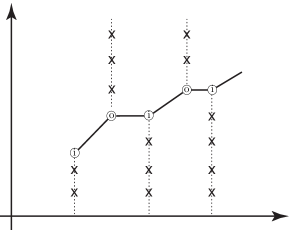
Figure 5.1. The inner corners are marked ⓘ and the outer corners are marked ⓞ. The exed out lines represent the inequalities $y^{\text{out}}_{n}\leq c_{X}(x^{\text{out}}_{n})$ and $c_{X}(x^{\text{in}}_{n})\leq y^{\text{in}}_{n}$. The properties of the embedding capacity function then imply that its graph consists of line segments between the corners.

Before we begin, it will be convenient to catalogue certain combinatorial identities that hold for our sequences. These will be essential for the inductive proofs that follow.

Lemma 5.2.

Let $X$ be a convex toric domain with negative weight expansion $(b;b_{1},\ldots,b_{n})$ equal to

$$(3)\ ,\ (3;1)\ ,\ (3;1,1)\ ,\ (3;1,1,1)\ ,\ (3;1,1,1,1)\ ,\mbox{or }(4;2,2).$$

When $J=2$, that is, for the sequences with recurrence relation $g(n+4)=Kg(n+2)-g(n),$ the following identities hold:

($$\clubsuit g(n)+g(n+2)=\beta_{n+1}g(n+1)$$)

($$\vardiamondsuit g(n)^{2}+g(n+2)^{2}-Kg(n)g(n+2)=-\alpha\beta_{n+1},$$)

($$\varheartsuit g(n)g(n+3)=g(n+1)g(n+2)+\alpha$$)

where $K=\text{vol}-2$, the sequence seeds, $\alpha$, and $\beta_{n}$ are:

Negative weight expansion	$K$	Seeds	$\alpha$	$\beta_{n}$
$(3)$	$7$	$2,1,1,2$	$3$	$3$
$(4;2,2)$	$6$	$1,1,1,3$	$2$	$\left\{\begin{array}[]{ll}2,&n\text{ odd}\\ 4,&n\text{ even}\end{array}\right.$
$(3;1,1,1)$	$4$	$1,1,1,2$	$1$	$\left\{\begin{array}[]{ll}2,&n\text{ odd}\\ 3,&n\text{ even}\end{array}\right.$
$(3;1,1,1,1)$	$3$	$1,2,1,3$	$1$	$\left\{\begin{array}[]{ll}1,&n\text{ odd}\\ 5,&n\text{ even}\end{array}\right.$

When $J=3$, that is, for the sequences with recurrence relation $g(n+6)=Kg(n+3)-g(n)$, the following identities hold:

($$\clubsuit g(n)+g(n+3)=\left\{\begin{array}[]{ll}g(n+1)+g(n+2),&n\equiv 0\mod 3\\ 2g(n+1)+g(n+2),&n\equiv 1\mod 3\\ g(n+1)+2g(n+2),&n\equiv 2\mod 3\\ \end{array}\right.$$ for (3;1))

($$\clubsuit g(n)+g(n+3)=\left\{\begin{array}[]{ll}g(n+1)+g(n+2),&n\equiv 0\mod 3\\ g(n+1)+2g(n+2),&n\equiv 1\mod 3\\ 2g(n+1)+g(n+2),&n\equiv 2\mod 3\\ \end{array}\right.$$ for (3;1,1))

($$\vardiamondsuit g(n)^{2}+g(n+3)^{2}-Kg(n)g(n+3)=-\beta_{n+1},$$)

($$\varheartsuit.1 g(n)g(n+4)=g(n+1)g(n+3)+\delta_{n}$$)

($$\varheartsuit.2 g(n)g(n+5)=g(n+2)g(n+3)+\mu_{n}$$)

where $K=\text{vol}-2$, the sequence seeds, $\beta_{n}$, $\delta_{n}$ and $\mu_{n}$ are:

Negative weight expansion	$K$	Seeds	$\beta_{n}$	$\delta_{n}$	$\mu_{n}$
$(3;1)$	$6$	$1,1,1,1,2,4$	$\left\{\begin{array}[]{ll}4,&n\equiv 1\mod 3\\ 7,&n\equiv 0,2\mod 3\end{array}\right.$	$\left\{\begin{array}[]{ll}1,&n\equiv 0,2\mod 3\\ 2,&n\equiv 1\mod 3\end{array}\right.$	$3$
$(3;1,1)$	$5$	$1,1,1,1,2,3$	$\left\{\begin{array}[]{ll}3,&n\equiv 1\mod 3\\ 5,&n\equiv 0,2\mod 3\end{array}\right.$	$1$	$\left\{\begin{array}[]{ll}2,&n\equiv 0,1\mod 3\\ 3,&n\equiv 2\mod 3\end{array}\right.$

Proof.

These identites can be proved by induction for each congruence class of $n$. For the $J=2$ cases it is useful to note that $\beta_{n}\beta_{n+1}=\text{vol}=K+2$. ∎

We now use the identities in Lemma 5.2 to establish the relationships among the the $x$- and $y$-coordinates of purported corners of the ellipsoid embedding functions.

Proposition 5.3.

The recurrence relations above define inner and outer corners respectively with coordinates:

$$(x^{\text{in}}_{n},y^{\text{in}}_{n})=\left(\frac{g(n+J)\left(g(n+1)+g(n+1+J)\right)}{\left(g(n)+g(n+J)\right)g(n+1)},\frac{g(n+J)}{g(n)+g(n+J)}\right),$$

$$(x^{\text{out}}_{n},y^{\text{out}}_{n})=\left(\frac{g(n+J)}{g(n)},\frac{g(n+J)}{g(n)+g(n+J)}\right).$$

These coordinates satisfy:

1. $\displaystyle{x^{\text{out}}_{n}<x^{\text{in}}_{n}<x^{\text{out}}_{n+1}}$ ;

2. $\displaystyle{\lim_{n\to\infty}x^{\text{out}}_{n}=\lim_{n\to\infty}x^{\text{in}}_{n}=a_{0}}$ ; and

3. $\displaystyle{\lim_{n\to\infty}y^{\text{out}}_{n}=\lim_{n\to\infty}y^{\text{in}}_{n}=\sqrt{\frac{a_{0}}{\text{vol}}}}$ .

Proof.

For (1): Both inequalities boil down to showing that

$$g(n+1)g(n+J)<g(n)g(n+J+1),$$

which follows immediately from the identities ($\varheartsuit$) in Lemma 5.2.

For (2): In view of (1), it suffices to show that $\displaystyle{\lim_{n\to\infty}x^{\text{out}}_{n}=a_{0}}$. The linear recurrence relation

$$g(n+2J)=Kg(n+J)-g(n)$$

is of order $2J$ but can be replaced by $J$ linear recurrence relations of order 2, one for each of the $J$ subsequences of $g(n)$ with $n\equiv j$ (mod $J$), for $j=0,1,\ldots,J-1$. Each of these subsequences has the recurrence relation

(5.4) $$g_{j}(n+2)=Kg_{j}(n+1)-g_{j}(n),$$

where $g_{j}(n)=g(Jn+j)$.

We can get a closed form for $g_{j}(n)$ by solving the polynomial equation $\lambda^{2}=K\lambda-1$. Let $\lambda_{1},\lambda_{2}$ be the roots of this equation, we note that in each of the cases we are considering we have $\lambda_{1}>1>\lambda_{2}>0$. Then for appropriate coefficients $D_{j},E_{j}$ depending on the seed of the sequences,

(5.5) $$g_{j}(n)=D_{j}\lambda_{1}^{n}+E_{j}\lambda_{2}^{n}.$$

For each $j=0,1,\ldots,J-1$ we have

$$\lim_{n\to\infty}\frac{g_{j}(n+1)}{g_{j}(n)}=\lim_{n\to\infty}\frac{D_{j}\lambda_{1}^{n+1}+E_{j}\lambda_{2}^{n+1}}{D_{j}\lambda_{1}^{n}+E_{j}\lambda_{2}^{n}}=\lambda_{1}.$$

Noting that $a_{0}$ is exactly $\lambda_{1}$, the larger solution of $\lambda^{2}-K\lambda+1=0$, we conclude as desired that $\lim_{n\to\infty}x_{n}=\lambda_{1}=a_{0}.$

Finally, for (3): In view of the fact that $y^{\text{out}}_{n}=y^{\text{in}}_{n}$, it suffices to show that

$$\lim_{n\to\infty}y^{\text{out}}_{n}=\sqrt{\frac{a_{0}}{\text{vol}}}.$$

Indeed we have

$$\lim_{n\to\infty}\frac{1}{y^{\text{out}}_{n}}=\lim_{n\to\infty}\left(\frac{1}{x^{\text{out}}_{n}}+1\right)=\frac{1}{a_{0}}+1=\sqrt{\frac{\text{vol}}{a_{0}}},$$

the last equality uses the facts that $a_{0}^{2}-Ka_{0}+1=0$ and $\text{vol}=K+2$. This completes the proof. ∎

Next, we show that at the outer corners, the ellipsoid embedding function is indeed obstructed in all of our six examples.

Proposition 5.6.

Let $X$ be a convex toric domain whose negative weight expansion $(b;b_{1},\ldots,b_{n})$ is

$$(3)\ ,\ (3;1)\ ,\ (3;1,1)\ ,\ (3;1,1,1)\ ,\ (3;1,1,1,1)\ ,\mbox{or }(4;2,2).$$

For each $(x^{\text{out}}_{n},y^{\text{out}}_{n})=\left(\frac{g(n+J)}{g(n)},\frac{g(n+J)}{g(n)+g(n+J)}\right)$, we have $y^{\text{out}}_{n}\leq c_{X}(x^{\text{out}}_{n})$.

Proof.

Recall that $N(a,b)_{k}$ denotes the $k^{\mathrm{th}}$ ECH capacity of $E(a,b)$ and $c_{k}(X)$ denotes the $k^{\mathrm{th}}$ ECH capacity of $X$. Let $k_{n}:=\frac{(g(n)+1)(g(n+J)+1)}{2}-1$. If we prove that

(5.7) $$g(n+J)\leq N(1,x^{\text{out}}_{n})_{k_{n}}\,\,\,\,\mbox{ and }\,\,\,\,g(n)+g(n+J)\geq c_{k_{n}}(X),$$

then we have the desired inequality:

$$y^{\text{out}}_{n}=\frac{g(n+J)}{g(n)+g(n+J)}\leq\frac{N(1,x^{\text{out}}_{n})_{k_{n}}}{c_{k_{n}}(X)}\leq\sup_{k}\frac{N(1,x^{\text{out}}_{n})_{k}}{c_{k}(X)}=c_{X}(x^{\text{out}}_{n}).$$

The first part of (5.7) can be rewritten as

$$g(n)g(n+J)\leq N(g(n),g(n+J))_{k_{n}},$$

and by Proposition 2.3 it is indeed true that there are at most $k_{n}$ terms of the sequence $N(g(n),g(n+J))$ strictly smaller than $g(n)g(n+J)$.

Next, we tackle the second part of (5.7):

$$g(n)+g(n+J)\geq c_{k_{n}}(X).$$

By Theorem 2.12, it suffices to find a convex lattice path $\Lambda_{n}$ that encloses $k_{n}+1$ lattice points and has $\Omega$-length equal to $g(n)+g(n+J)$:

(5.8) $$\mathcal{L}(\Lambda_{n})=\frac{(g(n)+1)(g(n+J)+1)}{2}\,\,\,\,\mbox{and}\,\,\,\,\ell_{\Omega}(\Lambda_{n})=g(n)+g(n+J).$$

We do this separately for each of the six cases under consideration in Appendix A.

The convex lattice paths $\Lambda_{n}$ for each case (and sub-case) can be found in Figure A.1, while the formulæ for $s_{n}$ and $t_{n}$ are provided in (A.2). Using the identities $(\vardiamondsuit)$ in Lemma 5.2 and induction we conclude that $s_{n}$ and $t_{n}$ are indeed integers.

Formulæ for the number of lattice points $\mathcal{L}(\Lambda_{n})$ enclosed by the path and its $\Omega$-length $\ell_{\Omega}(\Lambda_{n})$ are provided in Table A.5 for each case and sub-case. As discussed after Table A.5, it is a computational check that these give the correct numbers that satisfy (5.8). ∎

Next, we show that at the inner corners, there are explicit ellipsoid embeddings realizing the purported value of the ellipsoid embedding function. We do this by exploring recursive families of ATFs, following a suggestion of Casals. The idea that the recurrence sequences involved in the coordinates of the corners of the infinite staircases may be related to the Markov-type equations that show up when performing ATF mutations was first mentioned to us by Smith and is studied in detail by Maw for symplectic del Pezzo surfaces [44]. This procedure is explained nicely in Evans’ lecture notes [20, Example 5.2.4]. We use a series of mutations first described by Vianna [60, §3] on the compact manifolds corresponding to our negative weight expansions with $J=2$. The $J=3$ ATFs have base diagram a quadrilateral and do not seem to have been explicitly used before, though Vianna has introduced quadrilateral based ATFs in [60, Figs 7 and 8]. It could be interesting to explore the number theory and exotic Lagrangian tori that these produce. In algebraic geometry (and looking at the dual lattice), one can also study a related operation also called mutation, which is a combinatorial operation arising from the theory of cluster algebras. This is explored in [36]; in particular see Example 1.2 and references therein.

Proposition 5.9.

Let $X$ be a convex toric domain whose negative weight expansion is

$$(3)\ ,\ (3;1)\ ,\ (3;1,1)\ ,\ (3;1,1,1)\ ,\ (3;1,1,1,1)\ ,\mbox{or }(4;2,2).$$

For each $(x^{\text{in}}_{n},y^{\text{in}}_{n})=\left(\frac{g(n+J)\left(g(n+1)+g(n+1+J)\right)}{\left(g(n)+g(n+J)\right)g(n+1)},\frac{g(n+J)}{g(n)+g(n+J)}\right)$, there is a symplectic embedding

(5.10) $$E(1,x^{\text{in}}_{n}){\stackrel{{\scriptstyle s}}{{\hookrightarrow}}}y^{\text{in}}_{n}X,$$

which forces $c_{X}(x^{\text{in}}_{n})\leq y^{\text{in}}_{n}$.

Proof.

We use Theorem 1.3 and Proposition 2.27 to prove that there is an embedding

(5.11) $$E\left(\frac{g(n)+g(n+J)}{g(n+J)},\frac{g(n+1)+g(n+1+J)}{g(n+1)}\right){\stackrel{{\scriptstyle s}}{{\hookrightarrow}}}X,$$

which is equivalent to (5.10). By definition of $c_{X}(a)$, this implies the desired inequality. The proof consists of applying successive mutations to base diagrams, beginning with a Delzant polygon. This allows us to use Proposition 2.27 to find ellipsoids embedded in compact manifolds. Theorem 1.3 then allows us to deduce that those ellipsoids must also be embedded in the corresponding convex toric domain. Since two convex toric domains with the same negative weight expansions have identical ellipsoid embedding functions (see Remark 2.8), it suffices to exhibit the embeddings for one convex toric domain per negative weight expansion. We must take particular care with the negative weight expansion $(3;1,1,1,1)$, making use of Remark 3.3.

We begin by producing ATFs on the compact manifolds $M$ corresponding to our negative weight expansions. The manifolds are

$$\mathbb{C}P^{2}_{3}\ ;\ \mathbb{C}P^{2}_{3}\#\overline{\mathbb{C}P}^{2}_{1}\ ;\ \mathbb{C}P^{2}_{3}\#2\overline{\mathbb{C}P}^{2}_{1}\ ;\ \mathbb{C}P^{2}_{3}\#3\overline{\mathbb{C}P}^{2}_{1}\ ;$$

$$\mathbb{C}P^{2}_{3}\#4\overline{\mathbb{C}P}^{2}_{1}\ ;\ \mbox{and }\mathbb{C}P^{1}_{2}\times\mathbb{C}P^{1}_{2}.$$

Except for $\mathbb{C}P^{2}_{3}\#4\overline{\mathbb{C}P}^{2}_{1}$, these manifolds may be endowed with toric actions. The corresponding Delzant polygons are displayed in Figure 3.1. Our first step is to apply mutations to the Delzant polygons to produce a base diagram that is a triangle with two nodal rays when $J=2$ and a quadrilateral with three nodal rays when $J=3$. For $\mathbb{C}P^{2}_{3}\#4\overline{\mathbb{C}P}^{2}_{1}$, we use Vianna’s trick [60, §3.2] to find an appropriate ATF on this manifold. Specifically, we begin with the ATF on $\mathbb{C}P^{2}_{3}\#3\overline{\mathbb{C}P}^{2}_{1}$ given in Figure B.4(e). This ATF has a smooth toric corner at the origin where we may perform a toric blowup of symplectic size $1$, resulting in an ATF on $\mathbb{C}P^{2}_{3}\#4\overline{\mathbb{C}P}^{2}_{1}$. These initial maneuvers are described in Appendix B and the results are shown in Figure 5.12.

\begin{overpic}[scale={0.5},unit=1mm]{pregame-ATF-summary.pdf} \put(12.0,55.0){\tiny{$\mathbb{C}P^{2}_{3}$}} \put(58.0,55.0){\tiny{$\mathbb{C}P^{2}_{3}\#\overline{\mathbb{C}P}^{2}_{1}$}} \put(102.0,55.0){\tiny{$\mathbb{C}P^{2}_{3}\#2\overline{\mathbb{C}P}^{2}_{1}$}} \put(10.0,-3.0){\tiny{$\mathbb{C}P^{2}_{3}\#3\overline{\mathbb{C}P}^{2}_{1}$}} \put(55.0,-3.0){\tiny{$\mathbb{C}P^{2}_{3}\#4\overline{\mathbb{C}P}^{2}_{1}$}} \put(102.0,-3.0){\tiny{$\mathbb{C}P^{1}_{2}\times\mathbb{C}P^{1}_{2}$}} \end{overpic}

Figure 5.12. The base diagrams for ATFs on our manifolds. These are a triangle with two nodal rays when $J=2$ and a quadrilateral with three nodal rays when $J=3$.

We now want to show that for any $0<\varepsilon<1$,

(5.13) $$(1-\varepsilon)\cdot E\left(\frac{g(n)+g(n+J)}{g(n+J)},\frac{g(n+1)+g(n+1+J)}{g(n+1)}\right){\stackrel{{\scriptstyle s}}{{\hookrightarrow}}}M,$$

where $M$ is the compact manifold from our list. We achieve this by showing that the base diagram obtained at each additional mutation contains the triangle with vertices $(0,0)$, $\left(\frac{g(n)+g(n+J)}{g(n+J)},0\right),\left(0,\frac{g(n+1)+g(n+1+J)}{g(n+1)}\right)$. We proceed by induction. In Table 5.14, we record the additional data we will need for our recursive mutation procedure.

Negative weight expansion	$J$	$\sigma_{n}$
$(3)$	$2$	$1$
$(3;1,1,1)$	2	$\Bigg{\{}\begin{array}[]{ll}2,&n\text{ odd}\\ 3,&n\text{ even}\end{array}$
$(3;1,1,1,1)$	$2$	$\Bigg{\{}\begin{array}[]{ll}1,&n\text{ odd}\\ 5,&n\text{ even}\end{array}$
$(3;1)$	$3$	1
$(3;1,1)$	$3$	$\Bigg{\{}\begin{array}[]{ll}2,&n\equiv 0\mod 3\\ 1,&n\equiv 1,2\mod 3\end{array}$
$(4;2,2)$	$2$	$\Bigg{\{}\begin{array}[]{ll}1,&n\text{ odd}\\ 2,&n\text{ even}\end{array}$

Table 5.14. Additional data, by negative weight expansion.

We now treat separately the cases where $J=2$ and $J=3$, starting with $J=2$. In this case, starting with base diagrams in Figure 5.12 and continuing to apply mutations, all further base diagrams will be triangles. The induction hypothesis is that the triangle $\Delta_{n}$ has side lengths $a_{n},b_{n},c_{n}$, nodal rays $v_{n}$ and $u_{n}$ and hypotenuse direction vector $w_{n}$ as shown in Figure 5.15(a) , and that the matrix that takes $\Delta_{n}$ to $\Delta_{n+1}$ is $M_{n}$:

$$v_{n}=\begin{pmatrix}g(n+1)\\ -g(n+3)\end{pmatrix},\,\,\,u_{n}=\begin{pmatrix}-g(n)\\ g(n+2)\end{pmatrix},\,\,\,w_{n}=\begin{pmatrix}\sigma_{n+1}g(n+1)^{2}\\ -\sigma_{n+2}g(n+2)^{2}\end{pmatrix},$$

$$a_{n}=\frac{g(n+1)+g(n+3)}{g(n+1)},\,\,\,b_{n}=\frac{g(n)+g(n+2)}{g(n+2)},$$

$$\mbox{and }M_{n}=\begin{pmatrix}-\sigma_{n+2}\,g(n+2)^{2}&-\sigma_{n+1}\,g(n+1)^{2}\\ \sigma_{n+3}\,g(n+3)^{2}&2+\sigma_{n+2}\,g(n+2)^{2}\end{pmatrix},$$

where $\sigma_{n}$ is as in Table 5.14.

\begin{overpic}[scale={1},unit=1mm]{trianglen-bw.pdf} \put(12.0,32.0){{\small{$v_{n}$}}} \put(26.0,11.0){{\small{$u_{n}$}}} \put(35.0,39.0){{\small{$w_{n}$}}} \put(-3.0,28.0){\small{$a_{n}$}} \put(27.0,-2.0){\small{$b_{n}$}} \put(29.0,32.0){\small{$c_{n}$}} \put(26.0,-9.0){(a)} \end{overpic}

\begin{overpic}[scale={1},unit=1mm]{squaren-bw.pdf} \put(29.0,15.0){{\small{$u_{n}$}}} \put(19.5,27.0){{\small{$v_{n}$}}} \put(13.0,36.0){{\small{$w_{n}$}}} \put(49.0,30.0){{\small{$s_{n}$}}} \put(20.0,57.0){{\small{$r_{n}$}}} \put(-3.0,28.0){\small{$a_{n}$}} \put(27.0,-2.0){\small{$b_{n}$}} \put(42.0,25.0){\small{$c_{n}$}} \put(15.0,52.5){\small{$d_{n}$}} \put(26.0,-9.0){(b)} \end{overpic}

Figure 5.15. The general base diagrams (a) $\Delta_{n}$ for the cases when $J=2$; and (b) $\square_{n}$ for the cases when $J=3$.

The base case is immediate from Figure 5.12. For the induction step, we must check first that the matrix $M_{n}$ is indeed performing the mutation from $\Delta_{n}$ to $\Delta_{n+1}$, that is:

1. $M_{n}v_{n}=v_{n}$ ,

2. $M_{n}w_{n}=\begin{pmatrix}0\\ 1\end{pmatrix}$ , and

3. $\det(M_{n})=1$.

We must also check that this transformation gives rise to the new data of $\Delta_{n+1}$:

1. $w_{n+1}=M_{n}\begin{pmatrix}-1\\ 0\end{pmatrix}$ ,

2. $v_{n+1}=M_{n}u_{n}$ ,

3. $u_{n+1}=-v_{n}$ ,

4. $a_{n+1}=a_{n}+c_{n}$ ,

5. $b_{n+1}=a_{n}\,\frac{1^{\text{st}}\text{ entry of }v_{n}}{2^{\text{nd}}\text{ entry of }v_{n}}$ , and

6. $c_{n+1}=b_{n}-b_{n+1}$.

The proof of these uses the identities in Lemma 5.2. Finally, we note that at each step, the base diagram $\Delta_{n}$ is exactly the triangle with vertices $(0,0)$ , $(\frac{g(n)+g(n+2)}{g(n+2)},0)=(b_{n},0)$ and $(0,\frac{g(n+1)+g(n+3)}{g(n+1)})=(0,a_{n})$, which is what we wanted to prove.

Next we tackle the $J=3$ case. Here, the base diagram never becomes a triangle, instead it is always a quadrilateral. Figure 5.15(b) and the formulas below give the relevant data of the base diagram $\square_{n}$:

$$u_{n}=\begin{pmatrix}-g(n)\\ g(n+3)\end{pmatrix},\,\,\,w_{n}=\begin{pmatrix}g(n+1)\\ -g(n+4)\end{pmatrix},\,\,\,s_{n}=\begin{pmatrix}\sigma_{n+1}g(n+1)^{2}\\ 1-\sigma_{n+1}g(n+1)g(n+4)\end{pmatrix},\,\,\,r_{n}=\begin{pmatrix}\sigma_{n}g(n)g(n+3)-1\\ -\sigma_{n+3}g(n+3)^{2}\end{pmatrix},$$

$$a_{n}=\frac{g(n+1)+g(n+4)}{g(n+1)},\,\,\,b_{n}=\frac{g(n)+g(n+3)}{g(n+3)},$$

$$\mbox{and }M_{n}=\begin{pmatrix}1-\sigma_{n+1}\,g(n+1)g(n+4)&-\sigma_{n+1}\,g(n+1)^{2}\\ \sigma_{n+4}\,g(n+4)^{2}&1+\sigma_{n+1}\,g(n+1)g(n+4)\end{pmatrix},$$

where $\sigma_{n}$ is again as in Table 5.14.

Performing a mutation on $\square_{n}$ uses the matrix $M_{n}$ and yields $\square_{n+1}$. The matrix $M_{n}$ satisfies

1. $M_{n}w_{n}=w_{n}$

2. $M_{n}r_{n}=\begin{pmatrix}0\\ 1\end{pmatrix}$

3. $\det(M_{n})=1$

and the data for $\square_{n+1}$ is obtained via

1. $r_{n+1}=M_{n}s_{n}$

2. $s_{n+1}=M_{n}\begin{pmatrix}-1\\ 0\end{pmatrix}$

3. $v_{n+1}=M_{n}u_{n}$ and $w_{n+1}=M_{n}v_{n}$, or simply $w_{n+1}=M_{n}M_{n-1}u_{n-1}$

4. $u_{n+1}=-w_{n}$

5. $a_{n+1}=a_{n}+d_{n}$

6. $d_{n+1}=c_{n}$

7. $b_{n+1}=-a_{n}\,\frac{1^{\text{st}}\text{ entry of }w_{n}}{2^{\text{nd}}\text{ entry of }w_{n}}$

8. $c_{n+1}=b_{n}-b_{n+1}$.

The proof of these relations uses the identities in Lemma 5.2. Finally, we note that the triangle with vertices $(0,0)$ , $(\frac{g(n)+g(n+3)}{g(n+3)},0)=(b_{n},0)$ and $(0,\frac{g(n+1)+g(n+4)}{g(n+1)})=(0,a_{n})$ fits in the base diagram $\square_{n}$ for each $n$, which is what we wanted to prove.

The ATFs described above and Proposition 2.27 allow us to conclude that we have the desired embeddings (5.13) with target the compact manifold $M$. We now argue that there are also such embeddings with target a convex toric domain. Suppose that $X$ is the convex toric domain with the same negative weight expansion as $M$. By Theorem 1.3, we then have an embedding

$$(1-\varepsilon)\cdot E\left(\frac{g(n)+g(n+J)}{g(n+J)},\frac{g(n+1)+g(n+1+J)}{g(n+1)}\right){\stackrel{{\scriptstyle s}}{{\hookrightarrow}}}X$$

for every $0<\varepsilon<1$. Now note that

$$(1-\varepsilon)\cdot\overline{E(a,b)}\mathrel{\vbox{\hbox{\scalebox{2.0}{$\subset$}}}}\left(1-\frac{\varepsilon}{2}\right)\cdot E(a,b),$$

so we may conclude that we have symplectic embeddings of the closed ellipsoids

$$(1-\varepsilon)\cdot\overline{E\left(\frac{g(n)+g(n+J)}{g(n+J)},\frac{g(n+1)+g(n+1+J)}{g(n+1)}\right)}{\stackrel{{\scriptstyle s}}{{\hookrightarrow}}}X$$

for every $0<\varepsilon<1$. We may now apply [9, Cor. 1.6] to deduce that there is a symplectic embedding of the form (5.11), as desired. In fact, we may also apply Theorem 1.3 one more time to deduce that

$$E\left(\frac{g(n)+g(n+J)}{g(n+J)},\frac{g(n+1)+g(n+1+J)}{g(n+1)}\right){\stackrel{{\scriptstyle s}}{{\hookrightarrow}}}M.$$

Thus we have shown that there are ellipsoid embeddings representing the purported interior corners. ∎

We now have all of the ingredients in place to complete the proof that the Fano infinite staircases exist.

Proof of Theorem 1.16.

We know from Propositions 5.6 and 5.9 that $y^{\text{out}}_{n}\leq c_{X}(x^{\text{out}}_{n})$ and $c_{X}(x^{\text{in}}_{n})\leq y^{\text{in}}_{n}$.

Now we use Proposition 5.3. Since $x^{\text{out}}_{n}<x^{\text{in}}_{n}$ and $y^{\text{out}}_{n}=y^{\text{in}}_{n}$, because $c_{X}(a)$ is continuous and non-decreasing, it must be constant and equal to $y^{\text{out}}_{n}$ between $x^{\text{out}}_{n}$ and $x^{\text{in}}_{n}$. Furthermore, since $x^{\text{in}}_{n}<x^{\text{out}}_{n+1}$ and the points $(0,0)$, $(x^{\text{in}}_{n},y^{\text{in}}_{n})$ and $(x^{\text{out}}_{n+1},y^{\text{out}}_{n+1})$ are colinear, the scaling property of $c_{X}(a)$ implies that between each $x^{\text{in}}_{n}$ and $x^{\text{out}}_{n+1}$, the graph of $c_{X}(a)$ consists of a straight line segment (which extends through the origin). We thus have an infinite staircase in each of the cases studied.

Finally, by continuity and because $x^{\text{out}}_{n}\to a_{0}$, $x^{\text{in}}_{n}\to a_{0}$, and $y^{\text{out}}_{n}=y^{\text{in}}_{n}\to\sqrt{\frac{a_{0}}{\text{vol}}}$ as $n\to\infty$, we know that the infinite staircase accumulates from the left at $\left(a_{0},c_{X}(a_{0})=\sqrt{\frac{a_{0}}{\text{vol}}}\right)$, which completes the proof of the theorem. ∎

Remark 5.16.

One must take care to interpret the base diagrams in Figure 5.12 correctly. These represent almost toric fibrations on smooth manifolds, not moment map images of toric orbifolds.

6. Conjecture: why these may be the “only” infinite staircases

In this section we describe some evidence towards Conjecture 1.20, which speculates that the only rational convex toric domains that admit an infinite staircase are those whose moment polygon, up to scaling, is $AGL_{2}(\mathbb{Z})$-equivalent to one in Figure 1.8. In light of [3, 59] about infinite staircases for irrational targets, it is crucial in the conjecture that the toric domain be rational.

Let $X_{\Omega}$ be a rational convex toric domain with negative weight expansion $(b;b_{1},b_{2},\ldots,b_{n})$. The ellipsoid embedding function of the scaling of a convex toric domain is a scaling of the ellipsoid embedding function of the original domain. Thus, we may assume that the negative weight expansion of $X_{\Omega}$ is integral and primitive: $\gcd(b,b_{1},\dots,b_{n})=1$. With this scaling, we say that $\Omega$ is primitive.

By Theorem 1.11, if the ellipsoid embedding function of $X_{\Omega}$ has an infinite staircase, then $c_{X_{\Omega}}(a_{0})=\sqrt{\frac{a_{0}}{\text{vol}}}$. This implies that

$$E(1,a_{0}){\stackrel{{\scriptstyle s}}{{\hookrightarrow}}}\sqrt{\frac{a_{0}}{\text{vol}}}X_{\Omega},$$

which by Proposition 2.7 and conformality of ECH capacities is equivalent to an inequality of sequences of ECH capacities:

(6.1) $$c_{ECH}\left(E\left(\sqrt{\frac{\text{vol}}{a_{0}}},\sqrt{a_{0}{\text{vol}}}\right)\right)\leq c_{ECH}(X_{\Omega}).$$

To rewrite this inequality we introduce the cap function of a convex toric domain $X$, for $T\in\mathbb{N}$:

(6.2) $$\text{cap}_{X}(T)\;{:=}\;\#\{k:c_{k}(X)\leq T\}.$$

With $u=\sqrt{\frac{\text{vol}}{a_{0}}}$ and $v=\sqrt{a_{0}\text{vol}}$, the inequality (6.1) is equivalent to:

(6.3) $$\text{cap}_{E(u,v)}(T)\geq\text{cap}_{X_{\Omega}}(T),\mbox{ for all }T\in\mathbb{N}.$$

We first look at the right hand side of inequality (6.3). For rational convex toric domains $X_{\Omega}$ with $\Omega$ primitive, it is possible to argue that $\text{cap}_{X_{\Omega}}(T)$ has quadratic term $\frac{1}{2\text{vol}}T^{2}$ and linear term $\frac{\text{per}}{2\text{vol}}T$. In [61, Theorem 8], Wormleighton analyzes the constant term of $\text{cap}_{X_{\Omega}}(T)$ and shows that since $\Omega$ is a primitive lattice convex toric domain, the cap function of $X_{\Omega}$ is eventually equal to a quasipolynomial:

(6.4) $$\text{cap}_{X_{\Omega}}(T)=\frac{1}{2\text{vol}}T^{2}+\frac{\text{per}}{2\text{vol}}T+\Gamma_{r},$$

where $r\in\{0,\ldots,\text{vol}-1\}$ is a congruence class of $T$ (mod vol) and each $\Gamma_{r}$ is a constant.

Next, we look at the left hand side of inequality (6.3). For a general ellipsoid $E(u,v)$, the cap function equals the Ehrhart function of the triangle $\Delta_{u,v}$, with vertices $(0,0),(1/u,0),$ and $(0,1/v)$:

$$\text{cap}_{E(u,v)}(T) = \#\{k:c_{k}(E(u,v))\leq T\})$$

$$= \#\{k:N(u,v)_{k}\leq T\}$$

$$= \#\left(T\Delta_{u,v}\cap\mathbb{Z}^{2}\right)$$

$$= \text{ehr}_{\Delta_{u,v}}(T).$$

In the particular case of the ellipsoid in (6.3), it is usually the case that $a_{0}$ is irrational; since we are just explaining heuristic evidence, we assume this for what follows.

Assumption 6.5.

The accumulation point $a_{0}$ is irrational.

The case when $a_{0}$ is rational must be treated separately, and we will not concern ourselves with it here. With Assumption 6.5 in place, we have that the ratio $\frac{v}{u}=a_{0}$ is irrational, and thus we satisfy the conditions of [17, Lemma 2], which allows us to write:

(6.6) $$\text{cap}_{E(u,v)}(T)=\text{ehr}_{\Delta(u,v)}(T)=\frac{1}{2\text{vol}}T^{2}+\frac{\text{per}}{2\text{vol}}T+d(T),$$

where $d(T)$ is asymptotically $o(T)$. We use here the fact that (1.12) implies, via straight forward algebra,

(6.7) $$\frac{1}{u}+\frac{1}{v}=\frac{\text{per}}{\text{vol}}.$$

Now, modulo Assumption 6.5, if the ellipsoid embedding function of $X_{\Omega}$ has an infinite staircase, then (6.3) forces

(6.8) $$d(T)\geq\Gamma_{r},\mbox{ for all }T\in\mathbb{N}.$$

The converse would allow us to rule out the existence of infinite staircases by finding one $T$ for which

(6.9) $$d(T)<\Gamma_{r}.$$

Our approach for finding such a $T$ is partially inspired by influential work of Hardy and Littlewood [23, 24].

We say that a number $x$ has continued fraction expansion $[a_{0},a_{1},a_{2},\ldots]$ if

$$x=a_{0}+\frac{1}{a_{1}+\frac{1}{a_{2}+\frac{1}{\ddots}}}.$$

The numbers $a_{i}$ are called the partial quotients of $x$. Hardy and Littlewood studied the function $\text{ehr}_{\Delta_{u,v}}(T)$, as $T$ varies among the positive real numbers. They show in [23, Theorems A3 and A4] that if $\frac{u}{v}$ has bounded partial quotients, then the term $d(T)$ is $\mathcal{O}(\log(T))$. Moreover, they show that this is optimal in the sense that there is a positive constant $K$ and examples $\frac{u}{v}$ with bounded partial quotients that satisfy

(6.10) $$d(T_{i})>K\cdot\log(T_{i})\quad\mbox{ and }\quad d(T_{j})<-K\cdot\log(T_{j}),$$

where the $T_{i}$ and $T_{j}$ are two increasing sequences of real numbers. We will say that a function is optimally $\pm\mathcal{O}(\log(T))$ to signify that its behavior is $\mathcal{O}(\log(T))$ and it satisfies (6.10). In particular, if the $T_{j}$ could be assumed to be integers in (6.10), then (6.9) would eventually hold, since the $\Gamma_{r}$ are bounded. This would rule out infinite staircases for all rational convex toric domains, underscoring the subtlety of this argument.

In [17], Cristofaro-Gardiner, Li, and Stanley studied the function $\text{ehr}_{\Delta_{u,v}}(T)$ for integer values of $T$. They show that this function can sometimes be a quasipolynomial when restricted to integral $T$, even when $\frac{u}{v}$ is irrational, making both sides of (6.3) quasipolynomial. Being a quasipolynomial over $\mathbb{Z}$ implies that in contrast to (6.10) above, $d(T)$ only takes on finitely many values. They classify all cases where the Ehrhart function is a quasipolynomial as follows.

Theorem 6.11.

[17, Theorem 1(i)] Assume that $\frac{u}{v}$ is irrational. Then $\text{ehr}_{\Delta_{u,v}}(T)$ is a quasipolynomial if and only if

(6.12) $$u+v=\alpha\quad\mbox{ and }\quad\frac{1}{u}+\frac{1}{v}=\beta\quad\mbox{ for }\quad\beta\ ,\alpha\beta\ \in\mathbb{N}.$$

Remark 6.13.

In our context, following (4.11) and (6.7), we have $\alpha=\text{per}$ and $\beta=\frac{\text{per}}{\text{vol}}$.

In view of (6.10) and Theorem 6.11, we conjecture the following.

Conjecture 6.14.

Let $\frac{u}{v}$ be a quadratic surd such that $\frac{u}{v}+\frac{v}{u}\in\mathbb{Q}$ . If (6.12) does not hold, then $d(T)$ is optimally $\pm\mathcal{O}(\log(T))$ where the $T_{i}$ and $T_{j}$ are sequences of positive integers.

We will say more about why Conjecture 6.14 might hold below and now explain why Conjecture  6.14 and Assumption 6.5 imply Conjecture 1.20. Under these assumptions, if the ellipsoid embedding function of $X_{\Omega}$ has an infinite staircase then $\frac{\text{per}}{\text{vol}},\frac{\text{per}^{2}}{\text{vol}}$ are in $\mathbb{N}$. Consider now the convex toric domain $X_{\widetilde{\Omega}}$ corresponding to the scaled region $\widetilde{\Omega}=\frac{\text{per}}{\text{vol}}\Omega$. Because $\frac{\text{per}}{\text{vol}}\in\mathbb{N}$, the region $\widetilde{\Omega}$ is still a lattice polygon, with $\widetilde{\text{vol}}$ and $\widetilde{\text{per}}$ satisfying

$$\text{area}=\frac{\widetilde{\text{vol}}}{2}=\frac{\text{per}^{2}}{\text{vol}}\quad\mbox{ and }\quad\#\text{ of boundary lattice points}=\widetilde{\text{per}}=\frac{\text{per}^{2}}{\text{vol}}.$$

Pick’s Theorem states that

$$\text{area}=\#\text{ of interior lattice points}+\frac{\#\text{ of boundary lattice points}}{2}-1$$

and so we conclude that $\widetilde{\Omega}$ has exactly one interior lattice point: that is, it is a reflexive polygon. This completes our argument towards Conjecture 1.20.

We now complete our analysis of reflexive polygons. Up to $AGL_{2}(\mathbb{Z})$ equivalence there are exactly sixteen reflexive polygons: the twelve in Figure 1.8 plus the four in Figure 6.15, which have reduced blow-up vectors $(3;1,1,1,1,1)$ and $(3;1,1,1,1,1,1)$. Solving the quadratic equation (1.11) for these two negative weight expansions, we obtain that in the first case $a_{0}=1$ and in the second the quadratic equation has no real solutions at all. By Theorem 1.10, the latter case therefore can not have an infinite staircase. As for the former case, a straightforward modification of the method in [10, §2.5] can be used to show that $c_{X}(a)=\frac{a+1}{4}$ for $a\geq 1$ sufficiently close to $1$. Thus, infinite staircases do not exist in either of these cases.

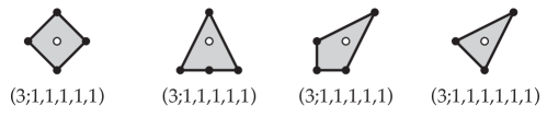
Figure 6.15. The remaining four reflexive polygons.

We close this section with some further exploration of Conjecture 6.14, showing how in general it follows from Conjecture 6.17. The general case is when $\alpha\beta=\frac{u}{v}+\frac{v}{u}+2\in\mathbb{Q}$ is not an integer, for $\alpha$ and $\beta$ defined by (6.12). In this context, $\alpha\beta=\frac{\text{per}^{2}}{\text{vol}}$, which is an invariant associated to the shape of the moment polygon $\Omega$ of the convex toric domain (up to scalings; see Remark 1.10). We start by examining $d(T)$. Following the analysis in Cristofaro-Gardiner, Li, and Stanley of Ehrhart functions for triangles, by [17, Eq. 2.1], $\text{ehr}_{\Delta_{u,v}}(T)$ can also be written as

$$\text{ehr}_{\Delta_{u,v}}(T)=\sum_{m=0}^{\lfloor{T/\text{per}}\rfloor}\left(1+\left\lfloor\frac{T-m\cdot\text{per}}{v}\right\rfloor+\left\lfloor\frac{T-m\cdot\text{per}}{u}\right\rfloor\right).$$

In what follows, we denote by $\{x\}=x-\lfloor x\rfloor$ the fractional part of a real number $x$. Let $T=n\cdot\text{per}$ and rewrite $\text{ehr}_{\Delta_{u,v}}(T)$ as

$$\text{ehr}_{\Delta_{u,v}}(n\cdot\text{per}) =\sum^{n}_{k=0}\left(1+\left\lfloor\frac{k\cdot\text{per}}{v}\right\rfloor+\left\lfloor\frac{k\cdot\text{per}}{u}\right\rfloor\right)$$ (Reindex.)

$$=2\sum^{n}_{k=0}k+\sum^{n}_{k=0}\left(1+\left\lfloor\frac{ku}{v}\right\rfloor+\left\lfloor\frac{kv}{u}\right\rfloor\right) \text{per}=u+v$$ (Use .)

$$=\left(2+\frac{u}{v}+\frac{v}{u}\right)\sum^{n}_{k=0}k-\sum^{n}_{k=0}\left(-1+\left\{\frac{ku}{v}\right\}+\left\{\frac{kv}{u}\right\}\right) \lfloor x\rfloor=x-\{x\}$$ (Note that .)

$$=\frac{\text{per}^{2}}{\text{vol}}\sum^{n}_{k=0}k-\sum^{n}_{k=0}\left(-1+\left\{\frac{ku}{v}\right\}+\left\{\frac{kv}{u}\right\}\right) \frac{u}{v}+\frac{v}{u}=\frac{\text{per}^{2}}{\text{vol}}-2$$ (Use .)

$$=\frac{\text{per}^{2}}{\text{vol}}\frac{\left(\frac{T}{\text{per}}\right)\left(\frac{T}{\text{per}}+1\right)}{2}-\sum^{n}_{k=0}\left(\left(\left\{\frac{ku}{v}\right\}-\frac{1}{2}\right)+\left(\left\{\frac{kv}{u}\right\}-\frac{1}{2}\right)\right)$$ (Compute the sum.)

$$=\frac{1}{2\text{vol}}T^{2}+\frac{\text{per}}{2\text{vol}}T-\sum^{n}_{k=0}\left(\left(\left\{\frac{ku}{v}\right\}-\frac{1}{2}\right)+\left(\left\{\frac{kv}{u}\right\}-\frac{1}{2}\right)\right).$$

For $n\in\mathbb{N}$ and $\theta\in\mathbb{R}\setminus\mathbb{Q}$, we define as in [5] the function

$$C_{\theta}(n):=\sum_{k=0}^{n}\left(\left\{k\theta\right\}-\frac{1}{2}\right).$$

Hardy and Littlewood established that $C_{\theta}(n)$ is optimally $\pm\mathcal{O}(\log(n))$ [24, Theorem 9]. The function $C_{\theta}\left(n\right)$ has a long history and has been studied by Sylvester [57], Lerch [38], Sierpiński [54], Hardy and Littlewood [23, 24] (who highlighted its properties in their 1912 ICM address), Ostrowski [51], Sós [55], and Brown and Shiue [5].

Comparing the final form of $\text{ehr}_{\Delta_{u,v}}(n\cdot\text{per})$ just above with (6.6), we conclude that for $T=n\cdot\text{per}$ we have

(6.16) $$d(T)=d(n\cdot\text{per})=-\left(C_{a_{0}}\left(n\right)+C_{1/a_{0}}\left(n\right)\right).$$

We conclude that, in the case when $\alpha\beta=a_{0}+\frac{1}{a_{0}}$ is not an integer, Conjecture 6.14 would now be a consequence of the following.

Conjecture 6.17.

Let $a_{0}$ be a quadratic surd such that $a_{0}+\frac{1}{a_{0}}\in\mathbb{Q}$. Then the function $C_{a_{0}}\left(n\right)+C_{1/a_{0}}\left(n\right)$ is bounded if and only if $a_{0}+\frac{1}{a_{0}}\in\mathbb{N}$. In particular, when it is bounded, it is identically zero. If it is unbounded, then it is unbounded above and below; and more specifically, it is optimally $\pm\mathcal{O}(\log(n))$.

Figure 6.18(a) and (b) shows some experimental evidence towards this conjecture. In (a), we have that $a_{0}+\frac{1}{a_{0}}$ is a natural number. In this case, the sum $C_{a_{0}}(n)+C_{1/a_{0}}(n)$ is identically zero on the domain computed. In (b), we have that $a_{0}+\frac{1}{a_{0}}=\frac{p}{q}$ is not a natural number. Here, the sum $C_{a_{0}}(n)+C_{1/a_{0}}(n)$ appears to be unbounded above and below. It takes on discrete values because it is always a multiple of $\frac{1}{q}$.

We include Figure 6.18(c) for contrast: here $a_{0}+\frac{1}{a_{0}}$ is irrational, more specifically, $a_{0}$ is the accumulation point $S_{2,0}$ for one of Usher’s infinite staircases [59]. This example is not in the scope of this manuscript because it does not correspond to a rational convex toric domain. The sum $C_{a_{0}}(n)+C_{1/a_{0}}(n)$ still appears to be unbounded above and below.

Sarnak has suggested two possible approaches for resolving Conjecture 6.17: an elementary approach involving continued fractions, along the lines of [5, 55]; or a more sophisticated approach building on results of Hecke’s [26]. This seems to us a good starting point for future work on this conjecture.

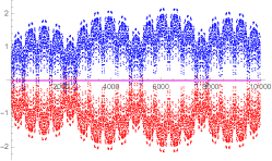
(a) $a_{0}+\frac{1}{a_{0}}=5$.

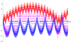
(b) $a_{0}+\frac{1}{a_{0}}=\frac{61}{9}$.

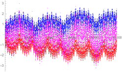
(c) $a_{0}+\frac{1}{a_{0}}=\frac{6+8\sqrt{3}}{3}$.

Figure 6.18. Each figure shows the function $C_{a_{0}}(n)$ in blue, the function $C_{1/a_{0}}(n)$ in red, and their sum $C_{a_{0}}(n)+C_{1/a_{0}}(n)$ in magenta.

Appendix A Lattice Paths

In this appendix, we compile the combinatorial data we need for Proposition 5.6.

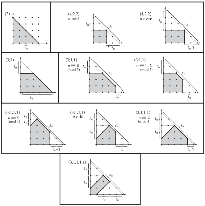
Figure A.1. The lattices paths $\Lambda_{n}$. All triangles drawn with size $s_{n}$ or $t_{n}$ on one of their sides are right-angle equilateral triangles (in the “length” that counts lattice points).

The sequences $s_{n}$ and $t_{n}$ that determine the paths $\Lambda_{n}$ have formulæ in terms of their negative weight expansions. In all six cases, the negative weight expansion is of the form $(B;b,\dots,b)$. In terms of those $B$ and $b$, we have

(A.2) $$s_{n}=\frac{B\cdot(g(n)+g(n+J))+c_{n}}{\text{vol}}\mbox{ and }t_{n}=\frac{b\cdot(g(n)+g(n+J))+d_{n}}{\text{vol}},$$

where $c_{n}$ and $d_{n}$ are given in Table A.4. We also have, in terms of $B$, $b$, and $k$ the number of $b$s,

(A.3) $$\ell_{\Omega}(\Lambda_{n})=B\cdot s_{n}+kb\cdot t_{n}+e_{n}.$$

The $e_{n}$ are given explicitly in Table A.4 and implicitly in Table A.5.

$(B;b,\dots,b)$	vol	$c_{n}$	$d_{n}$	$e_{n}$
$(3)$	$9$	$0$	$\nexists d_{n}$	0
$(4;2,2)$	$8$	$0$	$\begin{array}[]{ll}4&n\mbox{ even}\\ 0&n\mbox{ odd}\end{array}$	$\begin{array}[]{ll}2&n\mbox{ even}\\ 0&n\mbox{ odd}\end{array}$
$(3;1)$	$8$	$\begin{array}[]{rl}2&n\equiv 0\mod 6\\ -1&n\equiv 1\\ 1&n\equiv 2\\ -2&n\equiv 3\\ 1&n\equiv 4\\ -1&n\equiv 5\\ \end{array}$	$\begin{array}[]{rl}6&n\equiv 0\mod 6\\ -3&n\equiv 1\\ 3&n\equiv 2\\ -6&n\equiv 3\\ 3&n\equiv 4\\ -3&n\equiv 5\\ \end{array}$	0
$(3;1,1)$	$7$	$\begin{array}[]{rl}1&n\equiv 0\mod 6\\ -2&n\equiv 1\\ 2&n\equiv 2\\ -1&n\equiv 3\\ 2&n\equiv 4\\ -2&n\equiv 5\\ \end{array}$	$\begin{array}[]{rl}5&n\equiv 0\mod 6\\ -3&n\equiv 1\\ 3&n\equiv 2\\ 2&n\equiv 3\\ 3&n\equiv 4\\ -3&n\equiv 5\\ \end{array}$	$\begin{array}[]{rl}0&n\equiv 0\mod 3\\ 1&n\equiv 1,2\\ \end{array}$
$(3;1,1,1)$	$6$	$\begin{array}[]{rl}0&n\equiv 0\mod 4\\ 3&n\equiv 1\\ 0&n\equiv 2\\ -3&n\equiv 3\\ \end{array}$	$\begin{array}[]{rl}-2&n\equiv 0\mod 4\\ 3&n\equiv 1\\ 2&n\equiv 2\\ -3&n\equiv 3\\ \end{array}$	$\begin{array}[]{rl}-1&n\equiv 0\mod 4\\ 0&n\equiv 1,3\\ 1&n\equiv 2\\ \end{array}$
$(3;1,1,1,1)$	$5$	$\begin{array}[]{rl}4&n\equiv 0\mod 4\\ 0&n\equiv 1\\ -4&n\equiv 2\\ 0&n\equiv 3\\ \end{array}$	$\begin{array}[]{rl}3&n\equiv 0\mod 4\\ 0&n\equiv 1\\ -3&n\equiv 2\\ 0&n\equiv 3\\ \end{array}$	0

Table A.4. The constants $c_{n}$ and $d_{n}$ used in the formulæ in (A.2), by negative weight expansion; and the constants $e_{n}$ for (A.3).

$(B;b,\dots,b)$	$\mathcal{L}(\Lambda_{n})$	$\ell_{\Omega}(\Lambda_{n})$
$(3)$	$\frac{(s_{n}+1)(s_{n}+2)}{2}$	$3s_{n}$
$(4;2,2)$	$\begin{array}[]{ll}\frac{(s_{n}+1)(s_{n}+2)-t_{n}(t_{n}+1)-t_{n}(t_{n}-1)}{2}&n\mbox{ even}\\ \frac{(s_{n}+1)(s_{n}+2)-2\cdot t_{n}(t_{n}+1)}{2}&n\mbox{ odd}\end{array}$	$\begin{array}[]{ll}2(s_{n}-(t_{n}-1))+2(s_{n}-t_{n})&n\mbox{ even}\\ 2(s_{n}-t_{n})+2(s_{n}-t_{n})&n\mbox{ odd}\end{array}$
$(3;1)$	$\frac{(s_{n}+1)(s_{n}+2)-t_{n}(t_{n}+1)}{2}$	$2(t_{n})+3(s_{n}-t_{n})$
$(3;1,1)$	$\begin{array}[]{ll}\frac{(s_{n}+1)(s_{n}+2)-2\cdot t_{n}(t_{n}+1)}{2}&n\equiv 0\mod 3\\ \frac{(s_{n}+1)(s_{n}+2)-t_{n}(t_{n}+1)-t_{n}(t_{n}-1)}{2}&n\equiv 1,2\mod 3\end{array}$	$\begin{array}[]{ll}2t_{n}+3(s_{n}-2t_{n})+2t_{n}&n\equiv 0\mod 3\\ 2t_{n}+3(s_{n}-2t_{n}+1)+2(t_{n}-1)&n\equiv 1,2\mod 3\end{array}$
$(3;1,1,1)$	$\begin{array}[]{ll}\frac{(s_{n}+1)(s_{n}+2)-2t_{n}(t_{n}+1)-(t_{n}+1)(t_{n}+2)}{2}&n\equiv 0\mod 4\\ \frac{(s_{n}+1)(s_{n}+2)-3t_{n}(t_{n}+1)}{2}&n\equiv 1,3\mod 4\\ \frac{(s_{n}+1)(s_{n}+2)-2t_{n}(t_{n}+1)-(t_{n}-1)t_{n}}{2}&n\equiv 2\mod 4\end{array}$	$\begin{array}[]{ll}t_{n}+3(s_{n}-2t_{n}-1)+2(t_{n}+1)&n\equiv 0\mod 4\\ t_{n}+3(s_{n}-2t_{n})+2t_{n}&n\equiv 1,3\mod 4\\ t_{n}+3(s_{n}-2t_{n}+1)+2(t_{n}-1)&n\equiv 2\mod 4\end{array}$
$(3;1,1,1,1)$	$\frac{(s_{n}+1)(s_{n}+2)-4t_{n}(t_{n}+1)}{2}$	$t_{n}+3(s_{n}-2t_{n})+t_{n}$

Table A.5. The quantities $\mathcal{L}(\Lambda_{n})$ and $\ell_{\Omega}(\Lambda_{n})$, by negative weight expansion. The first, $\mathcal{L}(\Lambda_{n})$, counts lattice points enclosed by $\Lambda_{n}$. The second, $\ell_{\Omega}(\Lambda_{n})$, is a notion of length of the path, defined in (2.11); the constant term in each expression is $e_{n}$ in (A.3).

To prove Proposition 5.6, these quantities $\mathcal{L}(\Lambda_{n})$ and $\ell_{\Omega}(\Lambda_{n})$ must satisfy (5.8). Using the definitions of $s_{n}$ and $t_{n}$, as well as the properties $\heartsuit$ and $\clubsuit$ of Lemma 5.2, one can argue directly that $\mathcal{L}(\Lambda_{n})=\frac{(g(n)+1)(g(n+J)+1)}{2}$. We also have

$$\ell_{\Omega}(\Lambda)=B\cdot s_{n}+kb\cdot t_{n}+e_{n}=\frac{(B^{2}-kb^{2})(g(n)+g(n+J))+Bc_{n}-bkd_{n}}{\text{vol}}+e_{n}=g(n)+g(n+J)+\frac{Bc_{n}-bkd_{n}+\text{vol}\cdot e_{n}}{\text{vol}}.$$

Checking that $Bc_{n}-kbd_{n}+\text{vol}\cdot e_{n}=0$ for all cases and all moduli of $n$ then guarantees $\ell_{\Omega}(\Lambda)=g(n)+g(n+J)$, as desired.

Appendix B ATFs

In this appendix, we describe the initial ATF maneuvering required to produce ATFs on the manifolds

$$\mathbb{C}P^{2}_{3}\ ;\ \mathbb{C}P^{2}_{3}\#\overline{\mathbb{C}P}^{2}_{1}\ ;\ \mathbb{C}P^{2}_{3}\#2\overline{\mathbb{C}P}^{2}_{1}\ ;\ \mathbb{C}P^{2}_{3}\#3\overline{\mathbb{C}P}^{2}_{1}\ ;$$

$$\mathbb{C}P^{2}_{3}\#4\overline{\mathbb{C}P}^{2}_{1}\ ;\ \mbox{and }\mathbb{C}P^{1}_{2}\times\mathbb{C}P^{1}_{2}$$

that have base diagram a triangle with two nodal rays when $J=2$ and a quadrilateral with three nodal rays when $J=3$.

For $\mathbb{C}P^{2}_{3}$, $J=2$ and the moment image is already a triangle. We must simply apply nodal trades to add nodal rays at the two corners not at the origin. See Figure B.1.

\begin{overpic}[scale={0.5},unit=1mm]{3-pregame-atf.pdf} \put(20.0,-3.0){(a)} \put(70.0,-3.0){(b)} \end{overpic}

Figure B.1. In (a), we see the Delzant polygon for $\mathbb{C}P^{2}_{3}$. From (a) to (b), we have applied two nodal trades to add two singular fibers, creating a new almost toric fibration on $\mathbb{C}P^{2}_{3}$.

For $\mathbb{C}P^{2}_{3}\#\overline{\mathbb{C}P}^{2}_{1}$, $J=3$ and the moment image is already a quadrilateral. We must simply apply nodal trades to add nodal rays at the three corners not at the origin. See Figure B.2.

\begin{overpic}[scale={0.5},unit=1mm]{3-1-pregame-atf.pdf} \put(20.0,-3.0){(a)} \put(70.0,-3.0){(b)} \end{overpic}

Figure B.2. In (a), we see the Delzant polygon for $\mathbb{C}P^{2}_{3}\#\overline{\mathbb{C}P}^{2}_{1}$. From (a) to (b), we have applied three nodal trades to add three singular fibers, creating a new almost toric fibration on $\mathbb{C}P^{2}_{3}\#\overline{\mathbb{C}P}^{2}_{1}$.

For $\mathbb{C}P^{2}_{3}\#2\overline{\mathbb{C}P}^{2}_{1}$, $J=3$ and the moment image is a pentagon. There is a sequence of ATF moves that achieves a quadrilateral. See Figure B.3.

\begin{overpic}[scale={0.5},unit=1mm]{3-1-1-pregame-atf.pdf} \put(13.0,-3.0){(a)} \put(50.0,-3.0){(b)} \put(89.0,-3.0){(c)} \end{overpic}

Figure B.3. In (a), we see the Delzant polygon for $\mathbb{C}P^{2}_{3}\#2\overline{\mathbb{C}P}^{2}_{1}$. From (a) to (b), we have applied four nodal trades to add four singular fibers, creating a new almost toric fibration on $\mathbb{C}P^{2}_{3}\#2\overline{\mathbb{C}P}^{2}_{1}$. Finally, from (b) to (c), we apply a mutation, with resulting base diagram a quadrilateral with three nodal rays, as desired. In (c), two of the nodal rays have a single singular fiber and the third has two singular fibers. This is yet a third almost toric fibration on $\mathbb{C}P^{2}_{3}\#2\overline{\mathbb{C}P}^{2}_{1}$.

For $\mathbb{C}P^{2}_{3}\#3\overline{\mathbb{C}P}^{2}_{1}$, $J=2$ and the moment image is a hexagon. There is a sequence of ATF moves that achieves a triangle. See Figure B.4.

\begin{overpic}[scale={0.5},unit=1mm]{3-1-1-1-pregame-atf.pdf} \put(18.0,47.0){(a)} \put(55.0,47.0){(b)} \put(85.0,47.0){(c)} \put(24.0,-3.0){(d)} \put(75.0,-3.0){(e)} \end{overpic}

Figure B.4. In (a), we see the Delzant polygon for $\mathbb{C}P^{2}_{3}\#3\overline{\mathbb{C}P}^{2}_{1}$. From (a) to (b), we have applied five nodal trades to add five singular fibers, creating a new almost toric fibration on $\mathbb{C}P^{2}_{3}\#3\overline{\mathbb{C}P}^{2}_{1}$. From (b) to (c), we apply a mutation, with resulting base diagram a pentagon with four nodal rays. From (c) to (d), we apply another mutation, with resulting base diagram a quadrilateral with three nodal rays. Finally, from (d) to (e), we perform a third mutation, with resulting base diagram the desired triangle with two nodal rays. In (e), one of the nodal rays has two singular fibers and the other has three singular fibers.

For $\mathbb{C}P^{2}_{3}\#4\overline{\mathbb{C}P}^{2}_{1}$, $J=2$ but the manifold is not toric. We begin by using Vianna’s trick [60, §3.2] to find an appropriate ATF on this manifold. Specifically, we begin with the ATF on $\mathbb{C}P^{2}_{3}\#3\overline{\mathbb{C}P}^{2}_{1}$ given in Figure B.4(e). This ATF has a smooth toric corner at the origin where we may perform a toric blowup of symplectic size $1$. In terms of the base diagram, this corresponds to chopping off a $1\times 1$ triangle at the origin. This results in a quadrilateral with two nodal rays representing an ATF on $\mathbb{C}P^{2}_{3}\#4\overline{\mathbb{C}P}^{2}_{1}$, shown in Figure B.5(b). There is then a sequence of ATF moves that achieves a triangle with two nodal rays. See Figure B.5.

\begin{overpic}[scale={0.5},unit=1mm]{3-1-1-1-1-pregame-atf.pdf} \put(25.0,47.0){(a)} \put(78.0,47.0){(b)} \put(15.0,-3.0){(c)} \put(57.0,-3.0){(d)} \put(100.0,-3.0){(e)} \end{overpic}

Figure B.5. In (a), we see the base diagram for an ATF on $\mathbb{C}P^{2}_{3}\#3\overline{\mathbb{C}P}^{2}_{1}$. From (a) to (b), we have applied a toric blowup of size $1$ at the origin, resulting in an almost toric fibration on $\mathbb{C}P^{2}_{3}\#4\overline{\mathbb{C}P}^{2}_{1}$. From (b) to (c), we apply one nodal trade. From (c) to (d), we apply mutation, with resulting base diagram a quadrilateral with three nodal rays. Finally, from (d) to (e), we perform a second mutation, with resulting base diagram the desired triangle with two nodal rays. In (e), one of the nodal rays has one singular fiber and the other has five singular fibers.

For $\mathbb{C}P^{1}_{2}\times\mathbb{C}P^{1}_{2}$, $J=2$ and the moment image is a quadrilateral. There is a sequence of ATF moves that achieves a triangle, shown in Figure B.6

\begin{overpic}[scale={0.6},unit=1mm]{4-2-2-pregame-atf.pdf} \put(15.0,-3.0){(a)} \put(60.0,-3.0){(b)} \put(106.0,-3.0){(c)} \end{overpic}

Figure B.6. In (a), we see the Delzant polygon for $\mathbb{C}P^{1}_{2}\times\mathbb{C}P^{1}_{2}$. From (a) to (b), we have applied three nodal trades to add three singular fibers, creating a new almost toric fibration on $\mathbb{C}P^{1}_{2}\times\mathbb{C}P^{1}_{2}$. Finally, from (b) to (c), we apply a mutation, with resulting base diagram a triangle with two nodal rays, as desired. In (c), one of the nodal rays has a single singular fiber and the other has two singular fibers.

Appendix C Behind the scenes

In this section, we give an account of how we found the six negative weight expansions that appear in Theorem 1.16. At the beginning of this project, the ellipsoid embedding functions for the ball, polydisk, and ellipsoid $E(2,3)$ were known to have infinite staircases. These correspond to the blowup vectors $(1)$, $(4;2,2)$, and $(3;1,1,1)$.

By Theorem 1.11, we knew where the accumulation point would occur for any domain, if an infinite staircase were to exist. We wrote Mathematica code that generates an approximation of the graph of $c_{X}(a)$ for a given $X$, and started by trying a number different integer negative weight expansions. By chance, we first tried $(3;1)$ and found an infinite staircase. The vector $(3;1,1)$ admitted one too, and we were off, trying to prove that there was always an infinite staircase. The actual answer, of course, has turned out to be more subtle. The code we used in our early searches is included below and the notebook is available online at [14].

The idea behind the code is that the ellipsoid embedding function can be computed as the supremum of ratios of ECH capacities, as in equation (2.9). We compute a large (but finite!) number of ECH capacities of the domain $X$ using the sequence subtraction operation of Definition 2.4. We also compute a large but finite number of ECH capacities of $E(1,a_{i})$, for equally spaced values $a_{i}$ within a given range. Next, for each $a_{i}$ we find the maximum of the ratios of the computed ECH capacities, obtaining a list of points $(a_{i},\tilde{c}_{X}(a_{i}))$. Our code then approximates the graph by connecting the dots. Figure 1.14 illustrates four examples.

The graph of $\tilde{c}_{X}(a)$ is an approximation of the graph of the embedding function $c_{X}(a)$ in two senses: we are only using a finite number of points in the domain, and the the computed values $\tilde{c}_{X}(a_{i})$ are not completely accurate because we have restricted to a finite list of ECH capacities. Nonetheless, the approximation does allow us to visually rule out certain domains from the possibility of having an infinite staircase. For example, in the bottom left graph in Figure 1.14, there clearly exists an obstruction where the infinite staircase would have to accumulate, so that blowup vector must not admit an infinite staircase. In cases where it is more ambiguous, we change the range of points $a_{i}$, ask the code to compute more ECH capacities, and hence zoom in on the graph to probe further. For example, zooming in on the bottom right example in Figure 1.14 shows that in fact there exists an obstruction at the potential accumulation point.

Whenever this zooming in process suggested that there indeed exists an infinite staircase for that domain, the next step was to find the coordinates of the inner and outer corners of the staircase. Recall that in the ball case these are ratios of certain Fibonacci numbers, so we were interested in obtaining a recurrence sequence from the numerators and denominators of these coordinates. We used the Mathematica function Rationalize to approximate the values $\tilde{c}_{X}(a_{i})$ by fractions with small denominators and then fed the integer sequences obtained into OEIS, the Online Encyclopedia of Integer Sequences, sometimes unearthing unexpected connections. Eventually we switched to using the function FindLinearRecurrence on Mathematica to find the linear recurrence for the sequences found.

The Mathematica Code

     

List of first $\left(\frac{(\lfloor\frac{ka}{b}\rfloor+1)(k+1)}{2}-1\right)$ ECH capacities of the ellipsoid $E(a,b)$, we usually set $k=100$:

⬇

ECHellipsoid[a_, b_, k_] :=

Module[{l = Floor[(k + 1) Floor[1 + k a/b]/2] - 1},

Take[Sort[Flatten[Table[N[m a + n b], {m, 0, k}, {n, 0, k}]]], l]];

List of first $\left(\frac{(k-1)^{2}}{2}\right)$ ECH capacities of the ball $E(1,1)$, usually we set $k=100$:

⬇

ECHball[k_] :=

Take[Sort[Flatten[N[Array[Array[k - # &, #] &, k]]]],

Floor[(k - 1)^2/2]];

Sequence subtraction operation:

⬇

auxlist[list1_, list2_, i_] :=

Block[{a = list1, b = list2, l}, l = Min[Length[a], Length[b]];

Array[a[[i + #]] - b[[#]] &, l - i]];

minus[list1_, list2_] :=

Block[{a = list1, b = list2, l}, l = Min[Length[a], Length[b]];

Array[Min[auxlist[a, b, # - 1]] &, l]];

Ellipsoid embedding function $c_{X}(a)$ where ECHlist is (the beginning of) the sequence of ECH capacities of $X$:

⬇

c[a_, ECHlist_] := Module[{p = Length[ECHlist], k, l, nn},

k = Floor[(Sqrt[a^2 + 6 a + 1 + 8 a p] - 1 - a)/2];

nn = ECHellipsoid[1, a, k];

l = Min[p, Length[nn]];

Max[Array[nn[[# + 1]]/ECHlist[[# + 1]] &, l - 1]]];

Creates a list of points $(a_{i},c_{X}(a_{i}))$ where ECHlist is (the beginning of) the sequence of ECH capacities of $X$:

⬇

clist[amin_, amax_, astep_, ECHlist_] :=

Block[{l = Floor[(amax - amin)/astep]},

Array[{amin + (# - 1) astep, c[amin + (# - 1) astep, ECHlist]} &,

l]];

Plots the volume curve, plus a vertical line at the location of the potential accumulation point:

⬇

constraint[amin_, amax_, vol_, acc_] :=

Plot[Sqrt[t/vol], {t, amin, amax}, PlotStyle -> Red,

Epilog -> {InfiniteLine[{acc, 0}, {0, 1}]}];

Example C.1.

Let $X$ have negative weight expansion $(4;2,1)$. Make changes as necessary. Accpoint gives the location of the potential accumulation point, so that one can choose the range of points to plot. The output of this example is in Figure 1.14.

⬇

ECHcap = Block[{seq = ECHball[100]}, minus[minus[4*seq, 2*seq], seq]];

per = 3*4 - 2 - 1; (* per = 3 b - sum b_i *)

vol = 4^2 - 2^2 - 1^2; (* vol = b^2 - sum b_i^2 *)

accpoint = x /. NSolve[x^2 + (2 - per^2/vol ) x + 1 == 0, x][[2]]

5.17022

aamin = 1;

aamax = 6;

aastep = 0.01;

Show[{constraint[aamin, aamax, vol, accpoint],

ListPlot[clist[aamin, aamax, aastep, ECHcap], Joined -> True]}]

References

- [1] M. Audin, Torus actions on symplectic manifolds. Second revised edition. Progress in Mathematics 93. Birkhäuser Verlag, Basel, 2004.
- [2] M. Beck and S. Robins, “Computing the continuous discretely. Integer-point enumeration in polyhedra” second edition, Undergraduate Texts in Mathematics, Springer, New York, 2015.
- [3] M. Bertozzi, T. Holm, E. Maw, G. Mwakyoma, D. McDuff, A.R. Pires, and M. Weiler, “Infinite staircases for Hirzebruch surfaces”, arXiv:2010.08567.
- [4] P. Biran, “Symplectic packing in dimension 4”, GAFA, 7 (1997), 420 - 437.
- [5] T.C. Brown and P.J.-S. Shiue, “Sums of fractional parts of integer multiples of an irrational”, J. Number Theory 50 (1995), 181-192.
- [6] O. Buse, R. Hind, and E. Opshtein, “Packing stability for symplectic four-manifolds”, Trans. Amer. Math. Soc. 368 (2016), 8209-8222.
- [7] R. Casals and R. Vianna, “Sharp Ellipsoid Embeddings and Toric Mutations.” Preprint arXiv 2020.
- [8] K. Cieliebak, H. Hofer, J. Latschev, F. Schlenk. “Quantitative symplectic geometry.” Dynamics, ergodic theory, and geometry, 1–44, Math. Sci. Res. Inst. Publ., 54, Cambridge Univ. Press, Cambridge, 2007.
- [9] D. Cristofaro-Gardiner, “Symplectic embeddings from concave toric domains into convex ones”, with an Appendix by the author and K.Choi, J. Differential Geom. 112 (2019), 199-232.
- [10] D. Cristofaro-Gardiner, “Special eccentricities of four-dimensional ellipsoids.” Preprint arxiv 2020.
- [11] D. Cristofaro-Gardiner, D. Frenkel, and F. Schlenk, “Symplectic embeddings of four-dimensional ellipsoids into integral polydiscs.” Alg. Geom. Top. 17 (2017) 1189–1260.
- [12] D. Cristofaro-Gardiner and R. Hind, “Symplectic embeddings of products”, Comm. Math. Helv., 93 (2018), 1–32.
- [13] D. Cristofaro-Gardiner, R. Hind, D. McDuff, “The ghost stairs stabilize to sharp symplectic embedding obstructions”, J. Topology, 11 (2018), 309–378.
- [14] D. Cristofaro-Gardiner, T. S. Holm, A. R. Pires, and A. Mandini, Mathematica code, posted with the arXiv version of this manuscript.
- [15] D. Cristofaro-Gardiner, M. Hutchings, and V. Ramos, “The asymptotics of ECH capacities”, Invent. Math. 199 (2015), no. 1, 187–214.
- [16] D. Cristofaro-Gardiner and A. Kleinman, “Ehrhart polynomials and symplectic embeddings of ellipsoids.” JLMS, to appear. Preprint arXiv:1307.5493.
- [17] D. Cristofaro-Gardiner, T. Li, and R. Stanley, “New examples of period collapse.” Preprint arXiv:1509.01887.
- [18] D. Cristofaro-Gardiner and N. Savale, “Subleading asymptotics of ECH capacities.” Preprint arXiv:1811.00485.
- [19] M. Entov and M. Verbitsky, “Unobstructed symplectic packing for tori and hyperkahler manifolds”, J. Topol. Anal. 08, 589 (2016).
- [20] J. Evans, Lagrangian torus fibrations. Unpublished lecture notes http://jde27.uk/misc/ltf.pdf. dated 8 February 2019. Retrieved 22 January 2020.
- [21] D. Frenkel, D. Müller, “Symplectic embeddings of 4-dimensional ellipsoids into cubes.” J. Symplectic Geom. 13 (2015), no. 4, 765–847.
- [22] J. Gutt and M. Usher, “Symplectically knotted codimension-zero embeddings of domains in ”, Duke Math J., 168.12 (2019) 2299–2363.
- [23] G.H. Hardy and J.E. Littlewood, “Some problems of Diophantine approximation: The lattice-points of a right-angled triangle.” Proc. London Math. Soc. Ser. 2 20 no. 1378, (1920) 15–36.
- [24] G.H. Hardy and J.E. Littlewood, “Some problems of Diophantine approximation: The lattice-points of a right-angled triangle (second memoir).” Abh. Math. Sem. Hamburg 1 (1922), 212–249.
- [25] J.-C. Hausmann and A. Knutson, “A limit of toric symplectic forms that has no periodic Hamiltonians.” GAFA 10 (2000) 556–562.
- [26] E. Hecke, “Über analytische Funktionen und die Verteilung von Zahlen mod. eins.”, Abh. Math. Sem. Hamburg 1, 54-76 (1922).
- [27] R. Hind, “Some optimal embeddings of symplectic ellipsoids”, J. Topology, 8 (2015), 871–883.
- [28] R. Hind and E. Kerman, “New obstructions to symplectic embeddings”, Invent. Math., 196 (2014), 383–452.
- [29] T. Holm and L. Kessler, “Circle actions on symplectic 4-manifolds”, Comm. Ana. and Geo., 27.
- [30] M. Hutchings, “Recent progress on symplectic embedding problems.” Proc. Natl. Acad. Sci. USA 108 (2011), no. 20, 8093–8099.
- [31] M. Hutchings, “Quantitative embedded contact homology.” J. Differential Geom. 88 (2011), no. 2, 231–266.
- [32] M. Hutchings, “Fun with ECH capacities, II”, https://floerhomology.wordpress.com/2011/10/12/fwec2/.
- [33] M. Hutchings, “Lecture notes on embedded contact homology.” Contact and symplectic topology, 389–484, Bolyai Soc. Math. Stud., 26, János Bolyai Math. Soc., Budapest, 2014.
- [34] Y. Karshon, L. Kessler, and M. Pinsonnault, “A compact symplectic four-manifold admits only finitely many inequivalent toric actions”, J. Symp. Geom., 5 (2007) no. 2, 139–166.
- [35] Y. Karshon and E. Lerman, “Non-Compact Symplectic Toric Manifolds.” SIGMA. Symmetry Integrability Geom. Methods Appl. 11 (2015), Paper 055, 37 pp.
- [36] A. Kasprzyk and B. Wormleighton, “Quasi-period collapse for duals to Fano polygons: an explanation arising from algebraic geometry.” Preprint arXiv:1810.12472.
- [37] , J. Latschev, D. McDuff, and F. Schlenk, “The Gromov width of -dimensional torii”, Geom. Topol. 17.5, 2813-2853 (2013).
- [38] M. Lerch, “Question 1547’.’ L’Intermédiaire des mathématiciens 11 (1904), 144–145.
- [39] N.C. Leung and M. Symington, “Almost toric symplectic four-manifolds.” J. Symp. Geom. 8 (2010), no. 2, 143–187.
- [40] T.J. Li, “Smoothly embedded spheres in symplectic 4-manifolds”, Proc. AMS, 172.2, 609-613 (1999).
- [41] N. Magill and D. McDuff, “Staircase symmetries in Hirzebruch surfaces”, arXiv:2106.09143.
- [42] N. Magill, D. McDuff and M. Weiler, “Recursive staircase patterns for Hirzebruch surfaces”, in preparation
- [43] N. Magill, D. McDuff, and M. Weiler “Recursive patterns in Hirzebruch surfaces”, talk at Western Hemisphere Virtual Symplectic Seminar, July 2021, available online.
- [44] E. Maw, Symplectic topology of some surface singularities. PhD Thesis.
- [45] D. McDuff, “The structure of rational and ruled symplectic 4-manfolds”, J. Amer. Math. Soc 3 (1990), 679 - 712.
- [46] D. McDuff, “Symplectic embeddings of 4-dimensional ellipsoids.” J. Topol. 2 (2009), no. 1, 1–22.
- [47] D. McDuff, “The Hofer conjecture on symplectic embeddings of ellipsoids.” J. Diff. Geom. 88 (2011) 519–532.
- [48] D. McDuff, “A remark on the stabilized symplectic embedding problem for ellipsoids”, Eur. J. Math, 4 (2018) 356–371.
- [49] D. McDuff, “Hamiltonian - manifolds are uniruled”, Duke Math. J. 146 (3), 449 - 507.
- [50] D.McDuff, F.Schlenk, “The embedding capacity of 4-dimensional symplectic ellipsoids.” Ann. of Math. (2), 175 (2012), no. 3, 1191–1282.
- [51] A. Ostrowski, “Bemerkungen zur theorie der Diophantischen approximationen”, Abh. Math. Sem. Univ. Hamburg 1 (1922), 7.
- [52] K. Siegel, “Computing higher symplectic capacities I”, Preprint arXiv:1911.06466.
- [53] K. Siegel, “Higher symplectic capacities”, Preprint arXiv:1902.01490.
- [54] W. Sierpiński, “Pewne twierdzenie tyczace sie liczb niewymiernych - un théorème sur les nombres irrationnels”, Bull. Internat. Acad. Polon. Sci. Lett. Cl. Sci. Math. Naturelles Sér. A (Cracovie) (1909), 725-727.
- [55] V. T. Sós, “On the Theory of Diophantine Approximations I (on a problem of A. Ostrowski)”, Acta Math. 8 (1957), 461–472.
- [56] M.Steele, “The Cauchy-Schwarz Master Class” MAA Problem Books Series. Cambridge University Press, Cambridge, 2004. x+306 pp.
- [57] J.J. Sylvester, “Sur la fonction ”, Comptes Rendus, 50 (1860), 732–734 ( Collected math. papers, 2, 179–180).
- [58] M. Symington, “Four dimensions from two” Topology and geometry of manifolds (Athens, GA, 2001), Proc. Sympos. Pure Math. 71 153–208, Amer. Math. Soc., Providence, RI, 2003.
- [59] M. Usher, “Infinite staircases in the symplectic embedding problem for four-dimensional ellipsoids into polydisks” Algebr. Geom. Topol. 19 (2019), no. 4, 1935–2022.
- [60] R. Vianna, “Infinitely many monotone lagrangian tori in del Pezzo surfaces.” Selecta Math. (N.S.) 23 (2017), no. 3, 1955–1996.
- [61] Ben Wormleighton, “Algebraic capacities” Preprint arXiv:2006.13296.
- [62] N.T. Zung, “Symplectic topology of integrable Hamiltonian systems. II. Topological classification”, Compositio Math. 138 (2003) 125–156.