Chaotic solitons in driven sine-Gordon model

Abstract

Profiles of static solitons in one-dimensional scalar field theory satisfy the same equations as trajectories of a fictitious particle in multidimensional mechanics. We argue that the structure and properties of the solitons are essentially different if the respective mechanical motions are chaotic. This happens in multifield models and models with spatially dependent potential. We illustrate our findings using one-field sine-Gordon model in external Dirac comb potential. First, we show that the number of different “chaotic” solitons grows exponentially with their length, and the growth rate is related to the topological entropy of the mechanical system. Second, the field values of stable solitons form a fractal; we compute its box-counting dimension. Third, we demonstrate that the distribution of field values in the fractal is related to the metric entropy of the analogous mechanical system.

Keywords: solitons; dynamical chaos; sine-Gordon model; fractals; metric (Kolmogorov-Sinai) entropy; topological entropy.

1 Introduction and Summary

There exists an amusing mathematical analogy between static solitons in one-dimensional field theory and point-particle trajectories in multidimensional mechanics. Indeed, the solitonic profiles typically satisfy second-order equations [1, 2, 3]

$$\frac{\partial^{2}\varphi_{i}}{\partial x^{2}}=\frac{\partial V}{\partial\varphi_{i}}\;,$$ (1)

where $\varphi_{i}(x)$ are the fields of the model and $V(\varphi,\,x)$ is their scalar potential. These equations coincide with the Newton’s law for the evolution in “time” $x$ of a fictitious particle with coordinates $\varphi_{i}(x)$ in an external potential $V_{mech}\equiv-V$. Studying the mechanical trajectories, one can investigate the solitons. At $x\to\pm\infty$ the soliton fields approach the vacua — minima of the potential $V$. Thus, the respective mechanical trajectories $\varphi_{i}(x)$ lie on the separatrix: they start on the maximum of $V_{mech}(\varphi)$ at $x\to-\infty$ and climb onto the same or another maximum in the infinite “future”.

In this paper we argue on the basis of the above analogy that one-dimensional static solitons have essentially different properties in models with multiple fields or models with position-dependent potential $V(\varphi,\,x)$ as compared to the simplest case of a single-field scalar theory. Indeed, mechanical motions are typically chaotic in models with several degrees of freedom. Smooth separatrix in this case is destroyed [4], and the maxima of the potential $V_{mech}$ are connected by an infinite number of different trajectories. Since each trajectory represents the soliton, there exists an infinite number of the latter in the multifield models. Below we investigate such “chaotic” solitons and their distribution in the configuration space. Notably, we find that many of these objects are linearly stable from the viewpoint of field theory: they cannot be destroyed by adding a small perturbation and time-evolving the resulting configuration. The subset of stable solitons is of our primary interest.

To be specific, we consider sine-Gordon model [5] with coordinate-dependent potential [6, 7],

$$\varphi^{\prime\prime}=\frac{\partial V}{\partial\varphi}\;,\qquad\qquad V(\varphi,\,x)=U(x)\,\left(1-\cos\varphi\right),$$ (2)

where the prime represents $x$–derivative and $U(x)\geqslant 0$ is periodic. This model has vacua $\varphi_{n}=2\pi n$, where $n$ is integer. If $U$ is a constant, the analogous mechanical motion is one-dimensional, conservative, and therefore integrable. In this case there exist only two types of static solitons: “kink” $\phi_{K}(x)$ and “antikink” $\phi_{A}(x)$ interpolating between the neighbouring maxima of $V_{mech}\equiv-V$, see Fig. 1a. The profiles of these objects form smooth separatrix (Fig. 1b) in the mechanical “phase space” $(\varphi,\varphi^{\prime})$. Below we will consider nonintegrable case with spatially dependent $U(x)$.

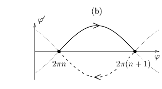
Figure 1: (a) Profiles of “kink” and “antikink” at constant $U$. (b) Respective trajectories in the mechanical “phase space” $(\varphi,\,\varphi^{\prime})$. The “time” $x$ grows along arrows.

It is worth noting that the sine-Gordon equation appears in several diverse setups. It describes relative phase difference between two coupled one-dimensional superfluids at low energies [14, 15, 16], rotation angle in classical ferromagnetic spin chain interacting with external magnetic field [17, 18, 19, 20], or phase of superconductors in long Josephson junction [21, 6, 7]. In all these cases inhomogeneous potential can be achieved by spatial variation of parameters: external electric or magnetic fields, or impurities between the superconductors [22].

In numerical calculations we use the simplest dependence of the potential (2),

$$U(x)=1+\varepsilon\sum\limits_{m=-\infty}^{\infty}\delta(x-mD)\,,$$ (3)

where $D=12$ is the period and the parameter $\varepsilon$ controls chaoticity of the underlying mechanical model. Although Eq. (3) may seem bizarre from the viewpoint of some applications, we expect that our results remain qualitatively valid for any periodic modulation. For the potential (3) the analogous mechanical motion is nearly integrable at $\varepsilon\lesssim 10^{-3}$. In this regime Kolmogorov-Arnold-Moser (KAM) theory of quasiperiodic motions [23, 24, 25] is applicable, and the “solitonic” trajectories remain close to the separatrix in Fig. 1b. In fact, they toss erratically from vacuum to vacuum along this separatrix. The respective solitons can be obtained by matching together the kink and antikink profiles, see Fig. 2a. The part of the “phase space” spanned by these trajectories, however, grows with $\varepsilon$ and fills a considerable region at $\varepsilon\gtrsim 0.1$. The solitons in the latter case appear in a wide variety of forms, see Fig. 2b.

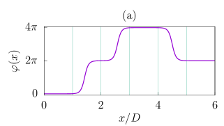
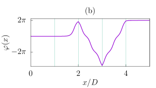
Figure 2: Examples of static solitons (a) in the KAM regime at $\varepsilon=3\times 10^{-7}$; (b) in the chaotic case at $\varepsilon=3$. Vertical lines mark positions of $\delta$-functions in Eq. (3).

In the main text we prove that the number of stable solitons $N_{sol}$ fitting in a finite spatial interval $0\leqslant x\leqslant L$ grows exponentially with the interval size,

$$N_{sol}\propto\mathrm{e}^{h_{S}(\varepsilon)\,L/D}\qquad\text{as}\qquad L\rightarrow+\infty,$$ (4)

where the growth rate $h_{S}(\varepsilon)$ monotonically increases with $\varepsilon$. The law (4) is demonstrated numerically in Figs. 3a, b. Steplike features of $h_{S}(\varepsilon)$ (arrows in Fig. 3b) result from new types of solitons emerging at larger $\varepsilon$.

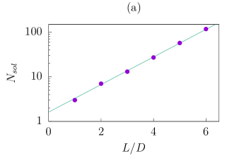
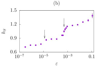
Figure 3: (a) The number of stable solitons $N_{sol}(L)$ in a finite spatial box as a function of the box size $L$. Numerical data (points) are fitted with Eq. (4) (line). (b) The logarithmic growth rate $h_{S}(\varepsilon)$ as a function of the chaoticity parameter $\varepsilon$.

Growth of the soliton multiplicity with $L$ can be easily explained in the KAM regime when the analogous mechanical motion proceeds along the smooth separatrix. In this case the stable solitons are completely specified by the set $\{\varphi_{n}\}$ of intermediate vacua. Say, the solitonic profile in Fig. 2a corresponds to the sequence $\{\varphi_{0},\,\varphi_{1},\,\varphi_{2},\,\varphi_{2},\,\varphi_{1}\}$. The number of possible sequences grows exponentially with their length $L/D$, and so does the number of stable solitons.

In the main text we demonstrate that the growth rate $h_{S}(\varepsilon)$ of stable solitons is bounded from above by the topological entropy $h_{T}(\varepsilon)$ of the analogous mechanical system [26, 27],

$$h_{S}(\varepsilon)\leqslant h_{T}(\varepsilon)\;.$$ (5)

The latter quantity characterizes complexity of the system i.e. diversity of its motions.

It is well-known that distinct classes of trajectories are separated by fractal sets in the phase space of chaotic systems [28, 29, 30, 31, 32]. We show that similarly, the solitons form a fractal in the space of static field configurations $\varphi(x)$. To visualize the fractal, we compute the field values $\varphi(0)$, $\varphi^{\prime}(0)$ of all stable solitons at a given spatial point $x=+0$ and plot them with dots in Fig. 4a. For example, the point S represents the soliton in Fig. 5a.

We find that the set in Fig. 4a is approximately self-similar. Indeed, it can be reproduced by magnifying a tiny region near one of its points, see Fig. 4b. To explain self-similarity, we choose points 1—3 in Fig. 4a and related points $1^{\prime}$—$3^{\prime}$ in Fig. 4b, then plot their profiles in Figs. 5b and 5c. Notably, at positive (or negative) $x$ the solutions $1^{\prime}$—$3^{\prime}$ go along $S$ first, then depart from it at $x\approx\pm 8D$ and follow the related profile 1, 2, or 3. Now, recall that the trajectory S is unstable from the mechanical viewpoint. Thus, small variations of its initial data $\varphi(0)$ and $\varphi^{\prime}(0)$ lead to variations of the new “initial data” at $x=8D$ enhanced by a factor $\mathrm{e}^{\lambda_{S}(8D)}$, where $\lambda_{S}(x)$ is related to the Lyapunov exponent of $S$. One concludes that a small vicinity of every point in Fig. 4a contains the entire set of “solitonic” Cauchy data squeezed by the Lyapunov factor $\mathrm{e}^{-\lambda_{S}}$.

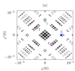
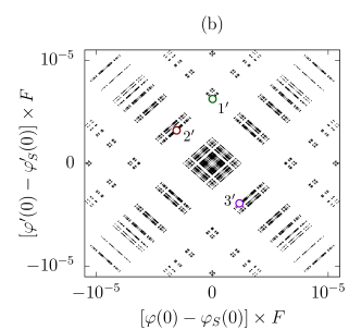
Figure 4: (a) Field values $\varphi(0)$, $\varphi^{\prime}(0)$ of stable solitons at $x=+0$ in the model with $\varepsilon=3\times 10^{-7}$. Only the region $|\varphi|,\,|\varphi^{\prime}|<10^{-5}$ is shown. (b) Field values in the vicinity of the point S in Fig. 4a magnified by a factor $F=\mathrm{e}^{\lambda_{S}(8D)}$, where $\lambda_{S}(8D)\approx 36.7$ is related to the Lyapunov exponent of the soliton $S$.

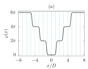
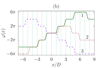
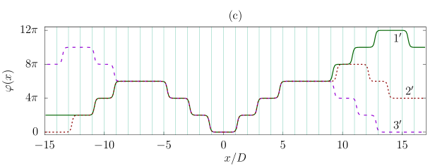
Figure 5: (a) The soliton with the Cauchy data S at $x=+0$, see Fig. 4a. (b) The solitons 1—3 corresponding to empty circles in Fig. 4a. (c) The related solitons $1^{\prime}$—$3^{\prime}$ with Cauchy data in Fig. 4b.

In Fig. 6 we plot the box–counting dimension [33, 34] $d(\varepsilon)$ of the “stable solitons” fractal in Fig. 4a at different values of the chaoticity parameter $\varepsilon$. Apparently, $d$ is not integer. Besides, it changes non-monotonically with $\varepsilon$ due to two competing effects. First, at larger $\varepsilon$ new solitons appear, increasing $d$. Second, Lyapunov exponents of already existing solitons grow with $\varepsilon$, making their field values closer in the $(\varphi,\varphi^{\prime})$ plane. This effect decreases $d$ at large $\varepsilon$.

In the main text we will demonstrate that at small $\varepsilon$ the fractal dimension $d(\varepsilon)$ is bounded from below by the stable solitons growth rate: $d(\varepsilon)\geqslant h_{S}(\varepsilon)/D$.

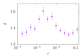
Figure 6: Box-counting dimension of the fractal in Fig. 4 at different $\varepsilon$.

An important characteristic of chaotic dynamics is the metric (Kolmogorov) entropy $K$. This quantity reflects divergence of the trajectories or, in other words, information growth rate during evolution [27]. Positive values of $K$ indicate chaos. We suggest field-theoretic analogue $E$ of this quantity characterizing the distribution of stable soliton field values $\varphi(0)$, $\varphi^{\prime}(0)$ at a given point $x=+0$. In particular, $E=0$ if all stable solitons have the same ${(\varphi,\,\varphi^{\prime})}$. Uniform distribution of solitonic field values gives $E=h_{S}$. In general case $E$ takes some value between these two limits, but it cannot exceed the Kolmogorov entropy of the underlying mechanical system, $E\leqslant K$. Thus, studying the soliton configurations one can investigate dynamical chaos in Eq. (1).

We perform explicit numerical computations only in the setup (2), (3). Nevertheless, we expect that the main qualitative properties of the solitons should be the same in other one-dimensional models with non-integrable static equations. Namely, the number of static solitons in these models should be infinite and the solitonic field values should form hierarchical structures in the configuration space. One can study the solitons using metric and topological entropies — the instruments originally developed for dynamical systems.

The paper is organized as follows. In Sec. 2 we introduce the model (2) and discuss its applications. The procedure of finding the solitons and determining their stability is described in Sec. 3. Soliton multiplicity and its relation to the topological entropy are considered in Secs. 4 and 5, respectively. The distribution of stable solitons in the configuration space is discussed in Sec. 6. The “solitonic” analogue of the metric entropy is suggested in Sec. 7. Section 8 is devoted to conclusions and discussion of possible generalizations.

2 The model: applications and properties

We consider the theory of one-dimensional static scalar field with energy

$$H[\varphi]=\int dx\left(\frac{1}{2}(\partial_{x}\varphi)^{2}+(1-\cos\varphi)U(x)\right),$$ (6)

where $U(x)$ is given by Eq. (3). By definition, the solitonic profiles extremize this energy at its finite values, i.e. satisfy Eq. (2). Stable solitons, in addition, correspond to local minima of $H[\varphi]$. They cannot be destroyed by adding a small perturbation and time-evolving the field in an energy-conserving way.

Let us describe several situations where Eqs. (6) and (2) appear. First, $(1+1)$-dimensional relativistic scalar field $\varphi(t,x)$ satisfies equation $\partial^{2}_{t}\varphi-\partial^{2}_{x}\varphi=-\partial V/\partial\varphi$ that reduces to (2) in the static case for a particular choice of the potential $V$, see [1, 2]. The function $U(x)$ is then a time-independent external field.

Second, one can consider Bose-Einstein condensate in the double well potential [14, 15, 16] forming two valleys stretched along the $x$ direction, see Fig. 7a. The condensates in the wells interact via tunneling through the potential barrier. It can be shown [14, 15, 16] that the relative phase difference $\varphi(x)=\arg\psi_{1}-\arg\psi_{2}$ of the condensate wavefunctions $\psi_{1},\psi_{2}$, satisfies (2), where $U$ characterizes coupling between the condensates. The spatial modulation can be introduced into this equation by periodically changing the barrier between the wells. Then the chaoticity parameter $\varepsilon$ in (2) is related to the modulation amplitude.

The third example is a classical ferromagnetic spin chain arranged along the $x$ axis [18, 19] and interacting with the external magnetic field $B$, as depicted in Fig. 7b. Long-range dynamics of this chain can be described [17, 20] by Eq. (2), where $\varphi(x)$ is a rotation angle of spins in the $y-z$ plane. In this case $U\propto B/\left(J_{s}\Delta^{2}\right)$, with $\Delta$ representing the interspin distance and $J_{s}$ characterizing interaction between the neighboring spins. Introducing spatial inhomogeneity into the magnetic field $B=B(x)$, we again obtain (2).

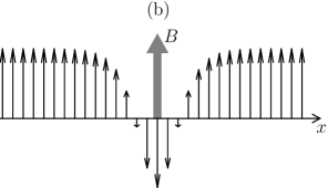
Figure 7: (a) Bose-Einstein condensate (thick solid lines) in a double-well potential with modulated coupling $U(x)$. (b) Ferromagnetic spin chain in a spatially inhomogenous magnetic field $B$.

There are many other applications of the static sine-Gordon equation (e.g. [21, 22]), where spatial modulation of the potential can be achieved by variation of external parameters. Keeping these applications in mind, below we consider general properties of static solitons in the model (2), (3) with $D=12$ and different $\varepsilon$.

The trivial solutions to Eq. (2) are the vacua $\varphi_{n}=2\pi n,n\in\mathbb{Z}$ corresponding to the absolute minima of energy (6) at all $\varepsilon$. In what follows we consider finite-energy solitons approaching these vacua at $x\rightarrow\pm\infty$.

To illustrate chaos in Eq. (2), we build the Poincaré sections [35] for the analogous mechanical system at different $\varepsilon$. To this end we consider a generic solution $\varphi(x)$ starting from the vacuum $\varphi\rightarrow 0$ at $x\rightarrow-\infty$. Numerically evolving the solution, we plot the values of $\varphi,\varphi^{\prime}$ at $x=mD+0$, i.e. after every period of the external potential, and obtain Fig. 8. At $\varepsilon=10^{-4}$ (Fig. 8a) the solution remains close to the smooth curve — the separatrix in Fig. 1b. In this case the analogous mechanical motion is nearly integrable. At $\varepsilon>10^{-3}$ (Fig. 8b) the values of $(\varphi,\varphi^{\prime})$ already form a sizeable “chaotic” region near the destroyed separatrix. At even larger $\varepsilon$ in Fig. 8c the solution $\varphi(x)$ tosses randomly inside the “phase space” covering a substantial part of it. Below we see how this chaos affects the soliton solutions in field theory.

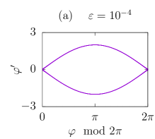
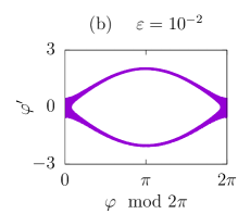
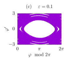
Figure 8: Poincaré sections at different $\varepsilon$. The values of $\varphi$ are taken modulo $2\pi$.

3 Computing the solitons

In this section we describe numerical method to find the solitons and determine their stability.

Since all vacua are equivalent, we consider only the solutions starting from $\varphi=0$ at ${x\rightarrow-\infty}$. Near the vacuum Eq. (2) becomes a linear Schrödinger equation in the periodic potential $U(x)$ [36]. General solution of this equation includes exponentially growing and decreasing parts,

$$\varphi\approx A\mathrm{e}^{\lambda_{v}x}f_{A}(x)+B\mathrm{e}^{-\lambda_{v}x}f_{B}(x)\,,$$ (7)

where $A,B$ are arbitrary constants, $\lambda_{v}=1+O(\varepsilon)>0$ is the Lyapunov exponent of the vacuum, and $f_{A,B}(x)$ are periodic; we normalize them by $f_{A,B}(0)=1$. We explicitly find $\lambda_{v}$ and $f_{A,B}$ in Appendix A. Clearly, all solitons starting from the vacuum at $x\rightarrow-\infty$ have $B=0$,

$$\varphi(x)\to A\,\mathrm{e}^{\lambda_{v}x}f_{A}(x)\quad\text{as}\quad x\to-\infty\,,$$ (8)

and we parametrize them with the shooting parameter $A$.

Analogously, the soliton profile arrives to some vacuum $\varphi_{n}$ at $x\to+\infty$, and its deviation from this vacuum is described by Eq. (7) with coefficients $A^{\prime}\equiv 0$ and arbitrary $B^{\prime}$. Taking the derivative of (7), we obtain the boundary condition

$$\varphi^{\prime}(x)=\left(-\lambda_{v}+\frac{f^{\prime}_{B}(x)}{f_{B}(x)}\right)(\varphi-\varphi_{n})\qquad\text{at}\qquad x\to+\infty.$$ (9)

In what follows we solve Eq. (2) with boundary conditions (8), (9).

We strongly rely on the shooting method. Imposing the boundary condition (8) at $x=0$, we numerically solve Eq. (2) for every $A$. Then we tune the value of $A$ to satisfy Eq. (9) at large $x=L$. Once this is done, we have all solitons localized inside the interval $0<x<L$.

In the chaotic regime our solutions are exponentially sensitive to the initial data. Thus, we need an efficient and extraordinary precise numerical method to solve Eq. (2). Our design of this method essentially relies on the simplified form of $U(x)$ in Eq. (3). Namely, in the regions between the $\delta$-functions $mD<x<(m+1)D$ the potential $U$ is constant and Eq. (2) can be solved explicitly in terms of elliptic functions, see Appendix B. At $x=mD$ one obtains matching conditions

$$\varphi(mD+0)=\varphi(mD-0),\qquad\varphi^{\prime}(mD+0)-\varphi^{\prime}(mD-0)=\varepsilon\sin\varphi(mD).$$ (10)

As a result, our algorithm acts sequentially. Starting from $\varphi$ and $\varphi^{\prime}$ at $x=mD+0$, it evolves them to $x=(m+1)D-0$ using the explicit solution in Appendix B, then performs matching (10) and proceeds to the next period of the potential.

Importantly, we perform all calculations using arbitrary precision floating numbers with $40\div 200$ digits. This gives us correct chaotic solutions of Eq. (2) of arbitrary complexity. The examples of these solutions are shown in Figs. 2 and 5. To study their statistical properties, below we obtain thousands of solitons of different forms and lengths.

We are mainly interested in stable static solitons. They correspond to local minima of energy (6). Adding small variation $\theta(x)$ to the solution $\varphi(x)$, one finds

$$H[\varphi+\theta]=H[\varphi]+\frac{1}{2}\int dx\,\theta(x)\hat{L}_{\varphi}(x)\theta(x)\,,$$ (11)

where $\hat{L}_{\varphi}(x)=-\partial^{2}_{x}+\cos\varphi(x)U(x)$. Thus, the soliton $\varphi(x)$ is stable if the operator $\hat{L}_{\varphi}$ is positive-definite in the space of perturbations $\theta(x)$ vanishing at $x\to\pm\infty$.

Numerically, we determine stability of solitons from the standard oscillation theorem. Namely, consider the perturbation

$$\theta_{0}(x)=\frac{\partial\varphi(x)}{\partial A}\,,$$ (12)

where $\varphi(x)$ is a solution of (2) with the initial data (8). By construction, $\theta_{0}(x)$ satisfies $\hat{L}_{\varphi}\theta_{0}=0$ and vanishes at $x\rightarrow-\infty$. Then by the oscillation theorem the number of its zeros equals the number of negative eigenvalues of the operator $\hat{L}_{\varphi}$. In numerical code we compute $\theta_{0}(x)$ for each soliton and count the number of its roots. The soliton is stable if $\theta_{0}(x)$ is positive-definite. In Appendix C we explain how this calculation can be conveniently performed within our shooting procedure.

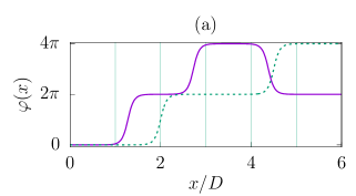
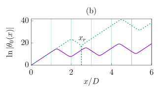
Figure 9: (a) Stable soliton (solid line) and unstable soliton (dashed line) at ${\varepsilon=4.5\times 10^{-5}}$. (b) Perturbations $\theta_{0}(x)$ of these solitons. Sharp cusp in the plot of unstable soliton perturbation at $x_{r}\sim 2.5D$ is its root.

Figure 9 shows the example of stable soliton (solid line), unstable soliton (dashed line) and their perturbations $\theta_{0}(x)$. Below we focus on stable solitons and prove that their number is infinite.

4 Multiplicity of solitons

There are only two static solitons in the pure sine-Gordon model: kink

$$\phi_{K}(x)=4\operatorname{arctan}\mathrm{e}^{x}$$ (13)

and antikink $\phi_{A}(x)=-\phi_{K}(x)$. The most general soliton solution includes spatial shifts of these two and a choice of the left vacuum: $\varphi=\phi_{K}(x-x_{K})+2\pi n$. It is impossible to combine kinks and antikinks in a static chain of solitons, since they interact with energy

$$E_{int}(s_{1},s_{2},R)=32s_{1}s_{2}\mathrm{e}^{-R}\,.$$ (14)

where $s_{\alpha}=+1$ for a kink, $-1$ for an antikink, and $R\gg 1$ is the distance between the solitons; see [3] and Appendix D. Indeed, widely separated kink and antikink accelerate towards each other, forming a breather, while two kinks or two antikinks repulse and go to infinity. In general, the leftmost and rightmost kinks in the solitonic chain cannot be at rest because each of them mostly interacts with the nearest neighbour.

To the leading order, small external potential ($\varepsilon\ll 1$) does not change the kink and antikink profiles, but affects weak forces between them. First, consider a single kink. Substituting ${\varphi_{k}(x)=\phi_{K}(x-x_{k})}$ into Eq. (6), we obtain a periodic potential

$$E_{\delta}(x_{k})\equiv H[\varphi_{k}]-M_{k}=2\varepsilon\sum\limits_{m\in\mathbb{Z}}\frac{1}{\cosh^{2}(mD-x_{k})}$$ (15)

which pulls the kink towards the equilibrium positions at $x_{k}=D(m+1/2)$; we introduced the kink mass $M_{k}=\int dx[(\partial_{x}\varphi_{k})^{2}/2+1-\cos\varphi_{k}]=8$. Note that at $D\gg 1$ all terms in the sum (15) are exponentially suppressed except for the two largest contributions from the closest $\delta$-functions of the external potential. In particular, the potential energy of the kink centered at $0<x_{k}<D$ approximately equals

$$E_{\delta}(x_{k})\approx 2\varepsilon\left(\frac{1}{\cosh^{2}(x_{k})}+\frac{1}{\cosh^{2}(D-x_{k})}\right)$$ (16)

with equilibrium at $x_{k}=D/2$.

Now, we add another kink or antikink inside the interval $lD<x^{\prime}_{k}<(l+1)D$. The total interaction energy of the soliton pair is now $E_{2}(x_{k},x^{\prime}_{k})=E_{\delta}(x_{k})+E_{\delta}(x^{\prime}_{k})\pm 32\mathrm{e}^{-(x^{\prime}_{k}-x_{k})}.$ It is clear that if $l$ is large enough, the interaction between the (anti)kinks is exponentially small, and they remain close to the original equilibrium positions at $x_{k}=D/2$ and ${x^{\prime}_{k}=(l+1/2)D}$. At small $l$ interaction between the solitons pulls them out of their potential wells, destabilizing the pair. Direct minimization of $E_{2}(x_{k},x^{\prime}_{k})$ shows that the kink-kink and kink-antikink pairs exist at

$$l>\frac{1}{D}\ln\frac{\varepsilon}{54}-1\qquad\text{and}\qquad l>\frac{1}{D}\ln\frac{\varepsilon}{2}+1,$$ (17)

respectively. Recall that the soliton pairs are not static in the original sine-Gordon model, so this is a new property that already can be traced back to the nonintegrability of the analogous mechanical system. Appearance of soliton pairs produces steps in the exponential growth rate of stable soliton multiplicity, see Fig. 3b. In particular, the leftmost arrow in this figure corresponds to the threshold $\varepsilon=2\mathrm{e}^{-D}$ for the existence of kink-antikink pair with $l=2$.

Let us demonstrate exponential growth of the stable soliton multiplicity with their length at small $\varepsilon$. To this end consider configuration of $N$ (anti)kinks,

$$\varphi=\sum_{\alpha=1}^{N}s_{\alpha}\varphi_{k}(x-x_{\alpha})\,,$$ (18)

where $s_{\alpha}=\pm 1$ distinguishes kinks from antikinks, and these objects are placed in the intervals $j_{\alpha}D<x_{\alpha}<(j_{\alpha}+1)D$. We will assume that distances between the adjacent (anti)kinks are large enough, so that the condition

$$j_{\alpha+1}-j_{\alpha}>p,\qquad\text{with}\qquad p=-\frac{1}{D}\ln\frac{\varepsilon}{32}+1$$ (19)

is satisfied. In this case the interaction energy (14) between the adjacent (anti)kinks ${|E_{int}|\leqslant 32\mathrm{e}^{-(p-1)D}}$ is at least twice smaller than their potential wells produced by the $\delta$-functions. This implies that the total energy of the chain has a local minimum with respect to the position of every kink, i.e. the stable equilibrium exists. Thus, the solitons can be arbitrarily added to the chain at distances exceeding $pD$.

We denote the number of the above “sparse” solitonic chains of length $lD$ or smaller by $N_{p}(l)$, where $l$ is an integer. In the larger interval of length $(l+p)D$ one can add a kink, an antikink or none of them to the chain. Thus, $N_{p}(l+p)\geqslant 3N_{p}(l).$ Using $N_{p}(1)=3$ as the initial condition, we find that $N_{p}(l)\geqslant 3^{(l+p-1)/p},$ i.e. the multiplicity of solitons grows at least exponentially with their length $lD$

On the other hand, the total number of solitons is bounded from above by the number $3^{l}$ of all possible soliton equilibrium positions with (anti)kinks occupying individual periods inside the interval $lD$. As a consequence, the number of stable solitons grows exponentially, see Eq. (4), and the growth rate $h_{S}$ is bounded by

$$\frac{\ln 3}{p}\leqslant h_{S}\leqslant\ln 3\,,$$ (20)

where $p$ was introduced in Eq. (19).

We numerically computed the number of stable solitons $N_{sol}(l)$ within the interval of length $lD$, see Fig. 3a. The multiplicity indeed grows exponentially, although the growth rate $h_{S}(\varepsilon)$ is much higher than our lower bound (20), see Figs. 3b and 10a.

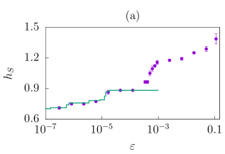
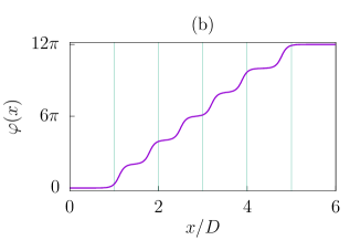
Figure 10: (a) Exponential growth rate $h_{S}(\varepsilon)$ of stable solitons. Points with errorbars are obtained by counting the number of numerically computed solitons. The solid line is found by minimizing the energy (21). (b) An example of the soliton at $\varepsilon=10^{-2}$ which is not represented by the ansatz (18).

The next step is to consider larger $\varepsilon$ corresponding to mostly chaotic dynamics of the analogous mechanical system, see Fig. 8b. In this case we use general expression for the energy of the solitonic chain,

$$E_{N}(x_{1},\ldots,x_{N})=\sum_{\alpha=1}^{N-1}E_{int}(s_{\alpha},s_{\alpha+1},x_{\alpha+1}-x_{\alpha})+\varepsilon\sum_{m}\left(\cos\left(\varphi(mD)\right)-1\right),$$ (21)

because when two (anti)kinks occupy adjacent periods of $U(x)$, they can affect each other’s interaction with the external potential. Minimizing (21) numerically with the conjugate gradient method, we determine whether a stable soliton chain exists for a given $\{s_{\alpha},j_{\alpha}\}$, where $j_{\alpha}D<x_{\alpha}<(j_{\alpha}+1)D$. The exponential growth rate obtained from numerical minimization of energy is shown by the solid line in Fig. 10a. It coincides with the exact graph at small $\varepsilon$, but starts to deviate from it at $\varepsilon\sim 10^{-3}$. This is due to the new types of solitons appearing in the system, with two or more (anti)kinks squeezed into one period of $U(x)$. The examples of such solitons are presented in Figs. 2b and 10b; the ansatz (18) is not valid for them. Not surprisingly, appearance of these solitons coincides with transition to chaos in the corresponding mechanical system, cf. Figs. 8b,c.

5 Topological entropy

An important quantity characterizing complexity of a dynamical system is the topological entropy [26]. In this section we define this quantity for the analogous mechanical system, then use it to constrain the soliton growth rate $h_{S}(\varepsilon)$.

Consider the solutions starting from $\varphi\to 0$ at $x\to-\infty$. Let us split the field values into segments

$$-\pi+2\pi n\leqslant\varphi\leqslant\pi+2\pi n.$$

We characterize every solution $\varphi(x)$ in the segment of length $lD$ with the sequence of regions $(n_{1},\ldots,n_{l})$ it visits after every period of $U(x)$, i.e. at $x=mD+0$. One can argue that the number of different sequences $N_{seq}(l)$ grows exponentially with the length of the interval $lD$. We therefore call

$$h_{T}=\lim_{l\to\infty}\,\frac{\ln N_{seq}(l)}{l}$$ (22)

the topological entropy of the analogous mechanical system.

The value of $h_{T}$ is an indicator of chaos. The above definition gives $h_{T}=0$ for ${\varepsilon=0}$. Indeed, solutions approaching the vacuum at $x\to-\infty$ include the vacuum itself and (anti)kinks at different positions, resulting in $2l+1$ sequences of length $l$. At small nonzero $\varepsilon$ the quantity $h_{T}$ is positive and bounded from below by the exponential growth rate $h_{S}$ of the soliton multiplicity. Indeed, every stable soliton corresponds to a unique sequence of visited vacua $(n_{1},\ldots,n_{l})$. Thus, $N_{sol}(l)\leqslant N_{seq}(l)$, implying (5).

6 Fractal structure

In this section we study the set of values $(\varphi(0),\varphi^{\prime}(+0))$ taken by the solitonic fields at $x=+0$. We consider a small vicinity of vacuum $|\varphi(0)|,|\varphi^{\prime}(+0)|\ll 1$. In this case the decomposition (7) applies at $x\approx+0$, where the first and second terms vanish exponentially at negative and positive $x$, respectively. Then the complete nonlinear solution can be represented as a sum $\varphi(x)\approx\varphi_{L}(x)+\varphi_{R}(x)$ of “left” and “right” parts vanishing at $x\to+\infty$ and $x\to-\infty$. In what follows we study only the “right” sector of solitons, with “left” solutions obtained by reflection $x\to-x$. In particular, if $\{\varphi_{\alpha}(x)\}$ is the set of “right” solitonic field values, the entire fractal in Fig. 4a consists of points

$$\varphi_{\alpha\beta}(0)=\varphi_{\alpha}(0)+\varphi_{\beta}(0),\qquad\varphi^{\prime}_{\alpha\beta}(+0)=\varphi^{\prime}_{\alpha}(+0)-\varphi^{\prime}_{\beta}(-0).$$ (23)

Details on computing the set of “right” solitons $\{(\varphi_{\alpha}(0),\varphi^{\prime}_{\alpha}(+0))\}$ are given in Appendix E.

Let us explain self-similarity of the fractal in Fig. 4. Suppose the “right” soliton $\varphi_{S}$ has parameter $A=A_{S}$ in Eq. (8) and length $lD$. Solution in its tiny vicinity can be represented as

$$\varphi_{A}(x)=\varphi_{S}(x)+(A-A_{S})\,\theta^{(S)}_{0}(x),$$

where $\theta^{(S)}_{0}$ is the perturbation (12) in the background of $\varphi_{S}(x)$. Taking ${A-A_{S}=\left[\theta^{(S)}_{0}(l^{\prime}D)\right]^{-1}}$ with $l^{\prime}>l$, one obtains the solution $\varphi_{A}(x)$ staying close to $\varphi_{S}(x)$, arriving to the same vacuum $\varphi_{n}$ and then departing from it at $x>l^{\prime}D$. At $x\approx l^{\prime}D$ the solution has the form $\varphi_{A}(x)\approx(A-A_{S})\,\theta^{(S)}_{0}(l^{\prime}D)\,f_{A}(x)\,\mathrm{e}^{x-l^{\prime}D}+\varphi_{n}$, where the asymptotics of $\theta^{(S)}_{0}(x)$ at $x\to+\infty$ was used. Thus, at $x=l^{\prime}D$ the boundary condition (8) is satisfied, with $(A-A_{S})\theta^{(S)}_{0}(l^{\prime}D)$ playing the role of the new parameter $A$. This mechanism is illustrated in Fig. 4b and the right parts of Figs. 5b, c. Note that the function $\lambda_{S}(x)\equiv\ln\left|\theta^{(S)}_{0}(x)\right|$ describes exponential growth of the perturbation and therefore is related to the Lyapunov exponent of the soliton $\varphi_{S}(x)$.

Now, let us compute the box-counting dimension of the fractal formed by the field values of solitons. To warm up, consider the entire set of solitons from the “right” sector, stable and unstable. This set is dense in the chaotic region, and its fractal dimension is $1$. Indeed, consider two close solutions $\varphi_{1}$ and $\varphi_{2}$ parametrized by $A_{1}$ and $A_{2}$. If the chaos is on, they diverge exponentially, with $|\varphi_{1}(x)-\varphi_{2}(x)|>2\pi$ at sufficiently large $x$. Then by continuity there exists a trajectory with parameter $A_{S}\in(A_{1},A_{2})$ that arrives precisely to the vacuum between $\varphi_{1}(x)$ and $\varphi_{2}(x)$. This trajectory is a soliton, which proves the statement.

The parameters ${A}$ of stable “right” solitons, however, form a Cantor-like set with fractal dimension less than $1$. Indeed, consider the soliton $\varphi_{S}(x)$ with $A=A_{S}$. We already argued that it contains the entire set of solitons in its arbitrarily small vicinity $|A-A_{S}|\ll 1$, and, in particular, unstable solitons. However, the solutions near the unstable solitons are also unstable: they also have roots of $\theta_{0}(x)$. Thus, the field values of stable soliton do not form a dense set, as their vicinities $|A-A_{S}|\ll 1$ contain infinitely many voids representing unstable solutions.

To compute the fractal dimension we use parameter

$$a=\dfrac{\ln A}{\lambda_{v}D}.$$ (24)

instead of $A>0$. Since $A(a)$ is a smooth function, this does not alter fractal dimension. Transformation $A\to A\mathrm{e}^{\lambda_{v}D}$ trivially shifts the solution by one period of the external potential and changes ${a\to a+1}$. Thus, the fractal is periodic in $a$; in what follows we consider only the segment $a\in[0,1)$. Dividing this segment into small boxes of size $\delta$, we count the number $N_{box}(\delta)$ of boxes with stable soliton parameters $\{a_{S}\}$ inside. The details on this procedure are given in Appendix E. The box-counting fractal dimension $d_{R}$ then can be extracted from the asymptotics

$$\ln N_{box}(\delta)\to-d_{R}\ln\delta\quad\text{as}\quad\delta\rightarrow 0.$$ (25)

The function $N_{box}(\delta)$ is shown in Fig. 11.

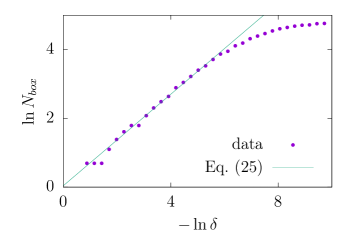
Figure 11: Number of boxes with stable solitons versus the box size at $\varepsilon=3\times 10^{-7}$. Fit with Eq. (25) (line) gives box-counting dimension $d_{R}=0.665\pm 0.020$.

Note that the fractal dimension can be analytically bounded from below. Consider the set of stable “right” solitons of length $lD$ or smaller. Perturbations $\theta_{0}(x)$ in their backgrounds grow with $x$ at a slower rate than the vacuum perturbations, $|\theta_{0}(x)|\leqslant\mathrm{e}^{\lambda_{v}x}|f_{A}(x)|$, simply because $\cos\varphi(x)$ in the equation $\hat{L}_{\varphi}\theta_{0}=0$ is maximal at $\varphi=2\pi n$. As a consequence, the solitons cannot have $A$ parameters at a distance closer than

$$\delta A_{l}=\left[\max\theta_{0}(x)\right]^{-1}\geqslant\mathrm{e}^{-\lambda_{v}lD},$$ (26)

where the maximum is taken within the interval $0\leqslant x\leqslant lD$. If Eq. (26) is not satisfied, the solitons would coincide in the entire interval. This gives the typical distance between the $a$ parameters of the solitons,

$$\delta a_{l}\gtrsim\mathrm{e}^{-\lambda_{v}lD}$$ (27)

for $A\lesssim O(1)$. Breaking the $a$-interval into the boxes (27), one obtains

$$d_{R}\geqslant\lim_{l\to\infty}\frac{\ln N_{sol}(l)}{-\ln\delta a_{l}}\geqslant\frac{h_{S}}{\lambda_{v}D},$$ (28)

where we used Eq. (4). Note that this bound is a serious underestimation: for ${\varepsilon=3\times 10^{-7}}$ it gives $d_{R}\gtrsim 0.06$, an order of magnitude smaller than the actual fractal dimension. Nevertheless, it proves that the dimension of our fractal is nonzero.

Since the fractal in Fig. 4 is a direct sum of “left” and “right” fractals, its dimension is $d(\varepsilon)=2d_{R}(\varepsilon)$, see Fig. 6.

7 Metric entropy

Metric (Kolmogorov-Sinai) entropy [27] is an important quantity indicating whether the dynamical system is chaotic or not. It was originally introduced for systems with compact phase space. Since our analogous mechanical system does not have this property [37], we first modify the entropy definition as follows.

We again restrict ourselves to the “right” solutions of length $L=lD$ starting from $\varphi\approx 0$ at $x=0$. Besides, we consider only a finite interval $|A|\leqslant A_{0}$ of their shooting parameter. We divide the phase space into strips:

$$2\pi\nu\leqslant\varphi+\varphi^{\prime}\left(\lambda_{v}-\frac{f^{\prime}_{B}(+0)}{f_{B}(0)}\right)^{-1}<2\pi(\nu+1)\,,$$ (29)

cf. Eq. (9). For every solution $\varphi(x)$ of length $lD$ we construct the sequence $\omega=(\nu_{1},\nu_{2},\ldots,\nu_{l})$ of visited regions at the start of every period $x=mD+0$. This divides the interval $-A_{0}\leqslant A\leqslant A_{0}$ of solution parameters into the regions $T_{\omega}$ corresponding to certain sequences. The solitons belong to the boundaries of $T_{\omega}$ due to Eq. (9). We define the metric entropy $K$ as

$$K_{l}=-\sum_{\omega}\frac{\Delta A\left(T_{\omega}\right)}{2A_{0}}\ln\left(\frac{\Delta A\left(T_{\omega}\right)}{2A_{0}}\right),\qquad\text{and}\qquad K=\lim\limits_{l\rightarrow+\infty}\frac{K_{l}}{l},$$ (30)

where $\Delta A(T_{\omega})$ is the total length of $T_{\omega}$. The only difference from the original Kolmogorov-Sinai construction is that we considered a selected set of trajectories and a particular sampling (29).

Note that at $\varepsilon=0$ only two non-trivial “right” solutions exist, the kink and the antikink, which belong to the regions with $\nu=0$ and $1$, respectively, at every $x$. We obtain only two sequences. Hence, $K=0$, as it should be in the integrable case.

Let us introduce the quantity analogous to the metric entropy considering the stable “right” solitons of length $L<lD$. Indeed, their shooting parameters divide the segment $-A_{0}\leqslant A\leqslant A_{0}$ into multiple intervals $R_{\alpha}$. We therefore define

$$E_{l}=-\sum_{\alpha}\frac{\Delta A\left(R_{\alpha}\right)}{2A_{0}}\ln\left(\frac{\Delta A\left(R_{\alpha}\right)}{2A_{0}}\right)\qquad\text{and}\qquad E=\lim_{l\rightarrow\infty}\frac{E_{l}}{l},$$ (31)

cf. (30). Clearly, $E$ characterizes (in)homogeneity of distribution of the stable soliton shooting parameters. If all solitons have the same $A$, then $E=0$. If they are evenly distributed, then $E_{l}=\ln N_{sol}(l)$ and $E=h_{S}$, see Eq. (4).

Since the boundaries of $R_{\alpha}$ are also the boundaries of $T_{\omega}$, splitting $\{R_{\alpha}\}$ is a coarse-graining of $\{T_{\omega}\}$ obtained by merging some of the regions together. However, if two regions of lengths $\Delta A_{1}$ and $\Delta A_{2}$ are merged into one,

$$-(\Delta A_{1}+\Delta A_{2})\ln\left(\frac{\Delta A_{1}+\Delta A_{2}}{2A_{0}}\right)\leqslant-\Delta A_{1}\ln\left(\frac{\Delta A_{1}}{2A_{0}}\right)-\Delta A_{2}\ln\left(\frac{\Delta A_{2}}{2A_{0}}\right).$$

This proves that $E_{l}\leqslant K_{l}$, and therefore $E\leqslant K$. In Fig. 12 we demonstrate the values of $E_{l}$, $K_{l}$ (points) and their linear fits (lines).

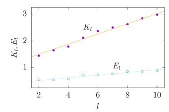
Figure 12: Values of $E_{l}$ and $K_{l}$ computed at $\varepsilon=3\times 10^{-7}$ and $A_{0}\approx 2.5\times 10^{-6}$. Linear fit gives $K=0.19\pm 0.01$ and $E=0.050\pm 0.004$.

Thus, one can use stable solitons in field theory to constrain metric entropy of the analogous mechanical system.

8 Generalization

In this paper we studied solitons in one-dimensional theories with nonintegrable static field equations. Specifically, we considered the sine-Gordon model in Dirac comb potential. This choice allowed us to implement an efficient numerical method for computing the multisoliton solutions. Due to the chaotic nature of the equations there exists an infinite set of these objects. Besides, we have found that the field values of the solitons form a fractal in the configuration space. We computed non-integer box-counting dimension of the fractal and studied it using the metric and topological entropies.

We do not want to leave an impression, however, that our model is special in some regard. Similar “chaotic” solitons should exist in many one-dimensional theories with non-integrable static equations, cf. [38, 39]. The simplest generalizations include one-field models with different periodically driven potentials $V(\varphi,x)$. If several $x$-independent degenerate vacua are present, these models possess topological solitons interpolating between the vacua. The soliton-counting method of this paper is then applicable if the periodic driving of the potentials is sufficiently weak and its period $D$ exceeds the width of the elementary “kink-like” solitons. In this case the number of solitons should grow exponentially with their length, and the solitonic field values should form self-similar fractals in the configuration spaces, just like in our model.

Another set of one-field models involves potentials $V(\varphi,x)$ with non-periodic spatial dependence. For example, one can consider the same driven sine-Gordon model, but with $\delta$-functions placed non-periodically in Eq. (3), at $x=x_{m}\neq mD$. If $\varepsilon$ is moderately small and the distance $x_{m+1}-x_{m}$ between the neighboring $\delta$-functions exceeds the kink width, the solitonic chains in this model can be constructed in the same way as in Sec. 4. Then there should exist an infinite number of stable solitons. Besides, their multiplicity should grow exponentially with the number $l$ of $\delta$-functions inside the soliton profile: expression (4) with $l$ in place of $L/D$. The field values of these solitons should form complicated hierarchical structures. However, self-similarity observed in Fig. 4 should be broken. Indeed, the argument of Sec. 6 relates magnifications of the soliton vicinity in the $\varphi(0),\varphi^{\prime}(0)$ plane to spatial translations of the soliton parts. If the discrete translation symmetry is broken, the self-similarity should disappear. Nevertheless, the box-counting fractal dimension of the set $\{\varphi(0),\varphi^{\prime}(0)\}$ may be non-integer.

An interesting special case is obtained by placing $\delta$-functions in Eq. (3) at random positions $x=x_{m}$. This may represent some kind of impurities in the original sample. Every realization of $\{x_{m}\}$ in this case corresponds to non-periodic $\delta$–comb. However, averaging over the random ensemble may essentially change the final properties of the solitons. The study of this notable case is beyond the scope of the present paper.

Let us point out that the results of this paper can be extended at least to some class of multifield models. Indeed, consider two fields $\varphi_{1}$ and $\varphi_{2}$ with the energy functional

$$H=\Gamma H_{1}[\varphi_{1}]+H_{2}[\varphi_{1},\varphi_{2}]\,,$$ (32)

where $\Gamma$ is a constant. Equations for the static solitons are

$$\frac{\delta H_{1}[\varphi_{1}]}{\delta\varphi_{1}}+\frac{1}{\Gamma}\frac{\delta H_{2}[\varphi_{1},\varphi_{2}]}{\delta\varphi_{1}}=0\,,\qquad\frac{\delta H_{2}[\varphi_{1},\varphi_{2}]}{\delta\varphi_{2}}=0\,.$$ (33)

At $\Gamma\gg 1$ the field $\varphi_{1}$ satisfies an independent equation, while $\varphi_{2}(x)$ evolves in the external potential $\varphi_{1}(x)$. If the latter is periodic, the properties of $\varphi_{2}$–solitons may be close to those in our model.

Generically, one expects to find an infinite total number of solitons in non-integrable case. But the distribution of the stable solitons may be model-dependent. Indeed, these solutions are the local minima of the static energy $H[\varphi]$ which coincides with the classical action in the mechanical analogy. Presently, there is no general classification of mechanical trajectories locally minimizing the action, though some works in this direction appear [40].

We hope that the instruments developed in this paper — metric and topological entropies, and fractals formed by field values — will be useful for studies of chaotic solitons in different theories.

Acknowledgements.

We are grateful to V. A. Rubakov for comments and criticism. This work was supported by the grant RSF 16-12-10494. Numerical calculations were performed on the Computational Cluster of the Theoretical Division of INR RAS.

Appendix A Deriving asymptotic conditions

Near the vacuum $\varphi=0$ Eq. (2) takes the form of a Schrödinger equation

$$\varphi^{\prime\prime}(x)=\varphi(x)U(x)$$ (34)

in the periodic potential $U(x)$, Eq. (3). The particular solutions of this equation coincide with the eigenfunctions of the shift operator $x\rightarrow x+D$. This suggests the ansatz

$$\varphi(x)=\mathrm{e}^{\lambda x}f(x)\,,$$ (35)

where $f(x)$ has period $D$. Solving Eq. (34) inside the interval $0<x<D$, one obtains,

$$f(x)=\mathrm{e}^{-\lambda x}(C_{+}\mathrm{e}^{x}+C_{-}\mathrm{e}^{-x})\,.$$ (36)

The linearized matching conditions (10) at the endpoints of this interval take the form

$$f(0)=f(D),\qquad f^{\prime}(D)+\varepsilon f(0)=f^{\prime}(0)\,,$$ (37)

where we recalled that $f$ is periodic. Substituting Eq. (36) into Eq. (37), we arrive to the homogeneous linear system

$$\left(\begin{matrix}\mathrm{e}^{(1-\lambda)D}-1&\mathrm{e}^{-(1+\lambda)D}-1\\ \varepsilon+\lambda-1+(1-\lambda)\mathrm{e}^{(1-\lambda)D}&\varepsilon+\lambda+1-(1+\lambda)\mathrm{e}^{-(1+\lambda)D}\end{matrix}\right)\left(\begin{matrix}C_{+}\\ C_{-}\end{matrix}\right)=0\,,$$ (38)

which has nontrivial solutions only if the matrix has zero determinant. This gives two roots

$$\lambda=\pm\frac{1}{D}\ln\left(\sigma+\sqrt{\sigma^{2}-4}\right)\equiv\pm\lambda_{v}\,,\qquad\sigma=\cosh D+\frac{\varepsilon}{2}\sinh D\,.$$ (39)

We obtained Eq. (7), where the particular solutions $f_{A}$, $f_{B}$ are given by Eq. (36) with $\lambda=\pm\lambda_{v}$ and coefficients $C_{+}$, $C_{-}$ representing the eigenvectors in Eq. (38). We normalize the solutions by $C_{+}+C_{-}=1$.

Appendix B General solution of the static sine-Gordon equation

In the regions between the $\delta$-functions Eqs. (2), (3) reduce to the equation for physical pendulum: $\varphi^{\prime\prime}=\sin\varphi$. The motion of the latter system depends on whether its mechanical energy

$$\mathscr{E}_{m}=\frac{\varphi^{\prime 2}}{2}+\cos\varphi-1$$ (40)

exceeds the height of the barrier $\mathscr{E}_{m}=0$ or not [41]. Periodic motions at $\mathscr{E}_{m}<0$ are described by general solution

$$\varphi(x)=2\operatorname{arccos}(\pm k\,\operatorname{sn}(x-x_{\pi},k))+2\pi n\,,\quad n\in\mathbb{Z}\,,$$ (41)

while the “rotating” solutions at $\mathscr{E}_{m}>0$ are

$$\varphi(x)=\pi\pm 2\operatorname{am}\left(k(x-x_{\pi}),\,\frac{1}{k}\right)\,.$$ (42)

Here $\operatorname{sn}$ and $\operatorname{am}$ denote the elliptic sine and Jacobi amplitude, respectively [42]. The solutions (41), (42) have two integration constants: $k=\sqrt{\mathscr{E}_{m}/2+1}$ and the shift parameter $x_{\pi}$. Signs $\pm$ in these equations discriminate two branches of solutions with opposite signs of $\varphi^{\prime}(x)$.

Numerically, we use Eqs. (41), (42) as follows. Starting with the values of $\varphi$ and $\varphi^{\prime}$ at $x=mD+0$, we compute $\mathscr{E}_{m}$, $k$, and determine the relevant branch of the general solution. Inverting Eq. (41) or (42), we find $x_{\pi}$ and hence — values of $\varphi$ and $\varphi^{\prime}$ within the entire interval ${mD<x<(m+1)D}$. Using the matching conditions (10), we proceed with the next interval.

Appendix C Linear stability

Let us describe a practical way to study soliton stability within the shooting approach. To this end we count zeros of the perturbation $\theta_{0}(x)$ in Eq. (12).

As the shooting parameter $A$ changes, these zeros cannot disappear or emerge sporadically inside the interval $0<x<L$. Indeed, one can regularize the $\delta$-functions in Eq. (3), making $\theta_{0}$ a smooth function of $x$ and $A$. After that the roots of $\theta_{0}$ can appear at the real axis or disappear from it only in pairs at points $x_{*}$ such that $\theta_{0}(x_{*})=\theta^{\prime}_{0}(x_{*})=0$. However, $\theta_{0}(x)$ is non-trivial and satisfies the second-order linear equation $\hat{L}_{\varphi}\theta_{0}=0$. It cannot vanish together with its first derivative at any $x$.

As a consequence, the number of $\theta_{0}$ roots inside the interval $0<x<L$ changes by $\pm 1$ when one of them crosses $L$. This happens at certain values $A=A_{*}$ of the shooting parameter satisfying $\partial\varphi(L)/\partial A=0$. Thus, we just need to find out whether the root $x_{r}(A)$ comes in or goes out of the interval. Differentiating the equality $\theta_{0}(x_{r}(A),A)=0$, we obtain the change $\Delta N_{r}$ in the number of roots,

$$\Delta N_{r}=-\operatorname{sgn}\left.\frac{dx_{r}}{dA}\right|_{A_{*}}=\operatorname{sgn}\left.\dfrac{\partial_{A}\theta_{0}(L)}{\theta^{\prime}_{0}(L)}\right|_{A_{*}}\,.$$ (43)

Expression (43) can be simplified using the mechanical energy $\mathscr{E}_{m}$, Eq. (40), which does not depend on $x$ inside the finite intervals $mD<x<(m+1)D$. Using Eq. (12), one finds $\partial_{x}\theta_{0}(L)=\partial_{x}\partial_{A}\varphi(L)=\partial_{A}\mathscr{E}_{m}/\varphi^{\prime}(L)$ at $A=A_{*}$. Therefore,

$$\Delta N_{r}=\left.\operatorname{sgn}\left(\partial_{A}\mathscr{E}_{m}\cdot\partial^{2}_{A}\varphi(L)\cdot\varphi^{\prime}(L)\right)\right|_{A_{*}}\,.$$ (44)

The factors in Eq. (44) can be computed numerically using the values of $\varphi$ and $\varphi^{\prime}$ at $x=L$ and different $A$. The latter are provided by the shooting method.

We apply Eq. (44) as follows. At small $A$ the solutions $\varphi_{A}(x)$ remain close to the vacuum, and $\theta_{0}(x)$ does not have zeros, $N_{r}=0$. We change $A$ in small steps and determine the values $A_{*}$ corresponding to $\partial_{A}\varphi(L)=0$. At these points we change the number of $\theta_{0}$ roots according to Eq. (44). Once all solitons are obtained, we select the stable ones, i.e. those with $N_{r}=0$.

We tested the above procedure by explicitly solving the equation $\hat{L}_{\varphi}\theta_{0}=0$ via the sequential algorithm, cf. Appendix B, arriving to the same result for the number of $\theta_{0}$ zeros.

Appendix D Interaction energy of a soliton pair

Consider a kink and an (anti)kink in the pure sine-Gordon model with centers separated by distance $R\gg 1$. This field configuration is approximated by a sum

$$\varphi_{2}(x)\equiv 4\arctan\mathrm{e}^{x+R/2}\pm 4\arctan\mathrm{e}^{x-R/2}=\varphi_{l}(x)\pm\varphi_{r}(x)\,,$$ (45)

where plus and minus signs correspond to kink and antikink at $x=R/2$, respectively. Substituting (45) into the energy (6) at $\varepsilon=0$, we find,

$$H=-16\int\limits_{-\infty}^{+\infty}\frac{dx(1\mp\cosh 2x)}{(\cosh 2x+\cosh R)^{2}}+\operatorname{const}=\pm 32\mathrm{e}^{-R}+O(\mathrm{e}^{-2R})+\operatorname{const},$$ (46)

where the constant includes all $R$-independent terms. In the last equality we computed the integrals and extracted the asymptotics $R\to\infty$, reproducing the well-known result [3].

Appendix E Finding the fractal to a given precision

In a nutshell, our numerical procedure for computing the fractal of “right” solitonic values (Sec. 6) is straightforward. We split the values of $a\in[0,1]$ into small boxes of size $\delta$, search for stable solitons within each box by the shooting method, and plot their field values with points in Figs. 4a,b. Changing the box size $\delta$, we obtain Fig. 11 and the coefficient in Eq. (25).

To calculate the fractal with resolution $\delta$, however, we need to search for the solitons of different length $L=lD$ in different $a$-boxes. We estimate $L$ by recalling that the difference between any two solutions grows exponentially with $x$: $\Delta\varphi\sim\Delta A\cdot\theta_{0}(x)\,.$ Thus, for a given soliton length $L$ we take the interval $\Delta A=\left[\theta_{\max}(L)\right]^{-1}$, where $\theta_{\max}(L)$ is the maximum of $|\theta_{0}(x)|$ at $0<x<L$. Solutions within this interval satisfy $\Delta\varphi\lesssim 1$, so it contains $O(1)$ stable solitons of length $L$, if they exist. Inversely, for a given $\Delta a=\delta$ we take large enough $L$ satisfying

$$\theta_{\max}(L)\geqslant\frac{1}{\Delta A}\geqslant\frac{\mathrm{e}^{-\lambda_{v}D\cdot a_{0}}}{\delta\cdot\lambda_{v}D}\,,$$ (47)

where in the last expression we converted $\Delta A$ into $\Delta a=\delta$ and used Eq. (24).

In practice we compute $\theta_{0}(x)$ for the solution in the center of each $a$-box to the point $x=L$ where Eq. (47) is already satisfied, then search for solitons of length $L$ within this box.

References

- [1] R. Rajaraman, “Solitons and Instantons. An Introduction to Solitons and Instantons in Quantum Field Theory,” Amsterdam: North-Holland (1982)
- [2] V. A. Rubakov, “Classical theory of gauge fields,” Princeton Univ. Press, 2002.
- [3] N. S. Manton and P. Sutcliffe, “Topological solitons,” Cambridge University Press, 2004.
- [4] G. M. Zaslavsky, “The physics of chaos in the Hamiltonian systems,” 2nd ed., Imperial College Press, 2007.
- [5] J. Cuevas-Maraver, P. G. Kevrekidis, F. Williams (eds.), “The Sine-Gordon Model and its Applications: From Pendula and Josephson Junctions to Gravity and High-Energy Physics,” Springer, 2014.
- [6] B. A. Malomed, V. A. Oboznov, A. V. Ustinov, “Supersolitons” in periodically inhomogeneous long Josephson junctions,” Sov. Phys. JETP 70, 518 (1990).
- [7] B. A. Malomed, “Superfluxons in periodically inhomogeneous long Josephson junctions,” Phys. Rev. B 41, 2616 (1990).
- [8] M. B. Fogel, S. E. Trullinger, A. R. Bishop, and J. A. Krumhansl, “Classical Particle-Like Behavior of Sine-Gordon Solitons in Scattering Potentials and Applied Fields,” Phys. Rev. Lett. 36, 1411 (1976) [Erratum-ibid 37, 314 (1976)].
- [9] M. B. Fogel, S. E. Trullinger, A. R. Bishop, and J. A. Krumhansl, “Dynamics of sine-Gordon solitons in the presence of perturbations,” Phys. Rev. B 15, 1578 (1977).
- [10] J. F. Currie, S. E. Trullinger, A. R. Bishop, and J. A. Krumhansl, “Numerical simulation of sine-Gordon soliton dynamics in the presence of perturbations,” Phys. Rev. B 15, 5567 (1977).
- [11] R. Scharf, Y. S. Kivshar, A. Sánchez, A. R. Bishop, “Sine-Gordon kink-antikink generation on spatially periodic potentials,” Phys. Rev. A 45, R5369 (1992).
- [12] A. Sánchez, R. Scharf, A. R. Bishop, and L. Vázquez, “Sine-Gordon breathers on spatially periodic potentials,” Phys. Rev. A 45, 6031 (1992).
- [13] W. Hai, Z. Zhang, and J. Fang, “Chaotic solitons in Sine-Gordon system,” Eur. Phys. J. B 21, 103 (2001).
- [14] N. K. Whitlock and I. Bouchoule, “Relative phase fluctuations of two coupled one-dimensional condensates,” Phys. Rev. A 68, 053609 (2003).
- [15] V. Gritsev, A. Polkovnikov, and E. Demler, “Linear response theory for a pair of coupled one-dimensional condensates of interacting atoms,” Phys. Rev. B 75, 174511 (2007) [arXiv:cond-mat/0701421].
- [16] T. Schweigler et al., ‘‘Experimental characterization of a quantum many--body system via higher--order correlations,’’ Nature 545, 323 (2017).
- [17] H. J. Mikeska, ‘‘Solitons in a one-dimensional magnet with an easy plane,’’ J. Phys. C 11, L29 (1978).
- [18] P. Kumar, V. K. Samalam, ‘‘Solitons in an easy-plane ferromagnetic chain,’’ J. Appl. Phys. 53, 1856 (1982).
- [19] G. Wysin, A. R. Bishop, and P. Kumar, ‘‘Soliton Dynamics on an Easy-Plane Ferromagnetic Chain,’’ J. Phys. C 17, 5975 (1984).
- [20] T. Kawasaki, ‘‘Dynamics Of Solitons In An Easy Plane Ferromagnetic Chain: A Discrete Lattice Model,’’ Prog. Theor. Phys. 75, 534 (1986).
- [21] S. A. Vasenko, K. K. Likharev, and V. K. Semenov, ‘‘Static properties of distributed inhomogeneous Josephson junctions,’’ Sov. Phys. JETP 54, 766 (1981).
- [22] D. W. McLaughlin and A. C. Scott, ‘‘Perturbation analysis of fluxon dynamics,’’ Phys. Rev. A 18, 1652 (1978).
- [23] V. I. Arnol’d, ‘‘Proof of a Theorem of A. N. Kolmogorov on the Preservation of Conditionally Periodic Motions under a Small Perturbation of the Hamiltonian,’’ Russ. Math. Surv. 18, 9 (1963).
- [24] V. I. Arnold, ‘‘Mathematical Methods of Classical Mechanics,’’ Springer, 1989.
- [25] J. Moser, ‘‘On Invariant Curves of Area-Preserving Mappings of an Annulus,’’ Nachr. Akad. Wiss. Göttingen Math.-Phys. Kl. II, 1 (1962).
- [26] R. L. Adler, A. G. Konheim, and M. H. McAndrew, ‘‘Topological Entropy,’’ Trans. Amer. Math. Soc. 114, 309 (1965).
- [27] E. Ott, ‘‘Chaos in Dynamical Systems,’’ Cambridge University Press, 2002.
- [28] E. Ott, ‘‘Strange attractors and chaotic motions of dynamical systems,’’ Rev. Mod. Phys. 53, 655 (1981).
- [29] D. K. Campbell, J. F. Schonfeld, and C. A. Wingate, ‘‘Resonance structure in kink-antikink interactions in theory,’’ Physica D 9, 1 (1983).
- [30] P. Anninos, S. Oliveira, and R. A. Matzner, ‘‘Fractal structure in the scalar theory,’’ Phys. Rev. D 44, 1147 (1991).
- [31] D. G. Levkov, A. G. Panin and S. M. Sibiryakov, ‘‘Complex trajectories in chaotic dynamical tunneling,’’ Phys. Rev. E 76, 046209 (2007) [arXiv:nlin/0701063].
- [32] T. Romańczukiewicz and Y. Shnir, ‘‘Oscillon resonances and creation of kinks in particle collisions,’’ Phys. Rev. Lett. 105, 081601 (2010) [arXiv:1002.4484].
- [33] J. Theiler, ‘‘Estimating fractal dimension,’’ J. Opt. Soc. Am. A 7, 1055 (1990).
- [34] N. Sarkar, B. B. Chaudhuri, ‘‘An efficient differential box-counting approach to compute fractal dimension of image,’’ IEEE Trans. Systems, Man, and Cybernetics 24, 115 (1994).
- [35] S. H. Strogatz, ‘‘Nonlinear Dynamics and Chaos,’’ Perseus Books, 1994.
- [36] V. I. Arnold, ‘‘Ordinary Differential Equations,’’ MIT Press, 1978.
- [37] S. F. Singer, ‘‘Symmetry in Mechanics: A Gentle, Modern Introduction," Birkhäuser, Boston, MA, 2004.
- [38] M. Yamashita, ‘‘Multisolitons and Soliton Lattices in Sine-Gordon System with Variable Amplitude,’’ Prog. Theor. Phys. 74, 622 (1985).
- [39] R. Scharf, A. R. Bishop, ‘‘Soliton chaos in the nonlinear Schrödinger equation with spatially periodic perturbations,’’ Phys. Rev. A 46, 2973 (1992).
- [40] C. G. Gray, E. F. Taylor, ‘‘When action is not least,’’ Am. J. Phys. 75, 434 (2007).
- [41] R. Z. Sagdeev, D. A. Usikov, G. M. Zaslavsky, ‘‘Nonlinear Physics, From the Pendulum to Turbulence and Chaos,’’ Harwood Academic Publishers, 1988.
- [42] F. W. Oliver, D. W. Lozier, R. F. Boisvert, C. W. Clark (eds.), ‘‘NIST Handbook of Mathematical Functions,’’ Cambridge University Press, 2010.