X-ray Binary Luminosity Function Scaling Relations in Elliptical Galaxies: Evidence for Globular Cluster Seeding of Low-Mass X-ray Binaries in Galactic Fields

Abstract

We investigate X-ray binary (XRB) luminosity function (XLF) scaling relations for Chandra detected populations of low-mass XRBs (LMXBs) within the footprints of 24 early-type galaxies. Our sample includes Chandra and HST observed galaxies at $D\lower 2.15277pt\hbox{$\;\buildrel<\over{\sim}\;$}25$ Mpc that have estimates of the globular cluster (GC) specific frequency ($S_{\_}N$) reported in the literature. As such, we are able to directly classify X-ray-detected sources as being either coincident with unrelated background/foreground objects, GCs, or sources that are within the fields of the galaxy targets. We model the GC and field LMXB population XLFs for all galaxies separately, and then construct global models characterizing how the LMXB XLFs vary with galaxy stellar mass and $S_{\_}N$. We find that our field LMXB XLF models require a component that scales with $S_{\_}N$, and has a shape consistent with that found for the GC LMXB XLF. We take this to indicate that GCs are “seeding” the galactic field LMXB population, through the ejection of GC-LMXBs and/or the diffusion of the GCs in the galactic fields themselves. However, we also find that an important LMXB XLF component is required for all galaxies that scales with stellar mass, implying that a substantial population of LMXBs are formed “in situ,” which dominates the LMXB population emission for galaxies with $S_{\_}N\lower 2.15277pt\hbox{$\;\buildrel<\over{\sim}\;$}2$. For the first time, we provide a framework quantifying how directly-associated GC LMXBs, GC-seeded LMXBs, and in-situ LMXBs contribute to LMXB XLFs in the broader early-type galaxy population.

1 Introduction

Due to its subarcsecond imaging resolution, Chandra has revolutionized our understanding of X-ray binary (XRB) formation and evolution by dramatically improving our ability to study XRBs in extragalactic environments (see, e.g., Fabbiano 2006 for a review). Extragalactic XRBs probe the compact object populations and accretion processes within parent stellar populations that can vary considerably from those represented in the Milky Way (MW; e.g., starbursts and massive elliptical galaxies). Low-mass XRBs (LMXBs) are of broad importance in efforts to understand XRBs, as they are the most numerous XRB populations in the MW (Grimm et al. 2002; Liu et al. 2007) and likely dominate the XRB emissivity of the Universe from $z\approx$ 0–2 (Fragos et al. 2013). With Chandra, these populations are readily resolved into discrete point sources in relatively nearby ($D\lower 2.15277pt\hbox{$\;\buildrel<\over{\sim}\;$}30$ Mpc) elliptical galaxies; however, there is still debate about their formation pathways.

LMXB populations are thought to form through two basic channels: (1) Roche-lobe overflow of normal stars onto compact-object companions in isolated binary systems that form in situ within galactic fields; and (2) dynamical interactions (e.g., tidal capture and multibody exchange with constituent stars in primordial binaries) in high stellar density environments like globular clusters (GCs; Clark 1975; Fabian et al. 1975; Hills 1976), and possibly some high-density galactic regions (e.g., Voss & Gilfanov 2007; Zhang et al. 2011). The “in-situ LMXBs” form on stellar evolutionary timescales (typically $\;\buildrel>\over{\sim}\;$1 Gyr) following past star-formation events. In contrast, the “GC LMXBs” form continuously over time as stochastic interactions between stars tighten binary orbits and induce mass transfer.

Since the early results from Uhuru, it has been known that the number of LMXBs per unit stellar mass coincident with GCs is a factor of $\sim$50–100 times larger than that observed for the Galactic field (Clark 1975; Katz 1975), clearly indicating the importance of the GC LMXB formation channel. GC LMXBs have been studied extensively in the literature, showing that stellar interaction rates and metallicity are the primary factors that influence the formation of these systems (see, e.g., Pooley et al. 2003; Heinke et al. 2003; Jordán et al. 2007; Sivakoff et al. 2007; Maxwell et al. 2012; Kim et al. 2013; Cheng et al. 2018).

Fewer studies have been able to explore the notable population of LMXBs that have been observed within galactic fields, which apparently trace the distributions of the old stellar populations (e.g., in late-type galaxy bulges and early-type galaxies). Given the very high formation efficiencies of GC LMXBs, and similarities in the X-ray properties of field versus GC LMXBs, it has been speculated that the field LMXB population may have also formed dynamically within GC environments, and then subsequently been planted within galactic fields, potentially through the ejection of LMXBs from GCs (Grindlay & Hertz 1985; Hut et al. 1992; Kremer et al. 2018) or the dissolution of GCs (e.g., Grindlay 1984). Several studies have confirmed strong correlations between the LMXB population emission per optical luminosity, $L_{\_}{\rm X}/L_{\_}{\rm opt}$, and the GC specific frequency: $S_{\_}N\equiv N_{\_}{\rm GC}10^{0.4(M_{\_}{V}^{T}+15)}$, which is the number of GCs per $V$-band luminosity (e.g., Irwin 2005; Juett 2005; Humphrey & Buote 2008; Boroson et al. 2011; Zhang et al. 2012). However, a non-zero intercept of the $L_{\_}{\rm X}/L_{\_}{\rm opt}$–$S_{\_}N$ correlation implied that a non-negligible population of LMXBs that are unassociated with GCs must be present and dominant at low-$S_{\_}N$, suggesting the in-situ formation channel is likely very important (e.g., Irwin 2005).

The majority of early Chandra studies of LMXB populations within elliptical galaxies investigated correlations between the total LMXB X-ray luminosity function (XLF) and host-galaxy stellar mass ($M_{\_}\star$) and were unable to segregate field versus GC sources directly (e.g., Kim & Fabbiano 2004; Gilfanov 2004; Humphrey & Buote 2008; Zhang et al. 2012). These investigations identified breaks in the LMXB XLF around 0.5–8 keV luminosities $L\approx 5\times 10^{37}$ erg s^-1 and $\approx 3\times 10^{38}$ erg s^-1, and showed that the XLF normalization increases with stellar mass and $S_{\_}N$. In the case of Zhang et al. (2012), a positive correlation was also observed between stellar age and $S_{\_}N$, indicating that stellar age may also be a driving physical factor.

Over the last decade, Chandra studies have directly isolated field LMXBs by removing X-ray sources with direct HST counterparts that are associated with either GCs or unrelated foreground stars, background galaxies, and active galactic nuclei (AGN; e.g., Kim et al. 2009; Voss et al. 2009; Paolillo et al. 2011; Luo et al. 2013; Lehmer et al. 2014; Mineo et al. 2014; Peacock & Zepf 2016; Peacock et al. 2017; Dage et al. 2019). These studies have found that the field LMXB XLF appears to have a steeper slope at $L\lower 2.15277pt\hbox{$\;\buildrel>\over{\sim}\;$}5\times 10^{37}$ erg s^-1 compared to the GC XLF and shows no obvious galaxy-to-galaxy variations among old elliptical galaxies, implying that the field LMXB population is dominated by sources formed via the in-situ channel. Furthermore, contrary to the findings of Zhang et al. (2012), Kim & Fabbiano (2010) and Lehmer et al. (2014) claimed an observed excess of luminous LMXBs in young elliptical galaxies with $\;\buildrel<\over{\sim}\;$5 Gyr stellar populations versus old elliptical galaxies with $\;\buildrel>\over{\sim}\;$8 Gyr. These findings have been supported by the observed increase in the average $L_{\_}{\rm X}$(LMXB)/$M_{\_}\star$ with increasing redshift among galaxy populations in deep Chandra surveys (see, e.g., Lehmer et al. 2007; 2016; Aird et al. 2017), and are consistent with population synthesis model predictions of the in situ LMXB XLF evolution with increasing host stellar population age (see, e.g., Fragos et al. 2008, 2013a, 2013b).

In this paper, we use the combined power of Chandra and HST data to provide new insight into the nature of the in-situ and GC formation channels, focusing on the field LMXB population. We study in detail a sample of 24 elliptical galaxies, using both archival and new data sets, with the aim of rigorously testing whether there is evidence for GC seeding or a stellar-age dependence in the field LMXB populations from XLFs. This represents a factor of three times larger study over any other published studies that analyze the GC and field LMXB population XLFs separately (i.e., compared to the eight galaxies studied by Peacock & Zepf 2016 and Peacock et al. 2017). In Section 2 we describe our sample selection. Section 3 provides details on the various multiwavelength, HST, and Chandra data analyses, and presents the properties of the galaxies and their X-ray point sources. Section 4 details our XLF fitting of the field, GC, and total LMXB populations, and culminates in a global XLF model framework that self-consistently fits the XLFs of all galaxies in our sample. In Section 5, we discuss and interpret our results and outline a way forward to establishing a universal physical parameterization of XRB XLFs. Full catalogs of the Chandra sources, Chandra images, and additional supplementary data sets are provided publicly and archived in Zenodo [doi: 10.5281/zenodo.3751108].

Throughout this paper, we quote X-ray fluxes and luminosities in the 0.5–8 keV bandpass that have been corrected for Galactic absorption, but not intrinsic absorption. Estimates of $M_{\_}\star$ and SFR presented throughout this paper have been derived assuming a Kroupa (2001) initial mass function (IMF); when making comparisons with other studies, we have adjusted all values to correspond to our adopted IMF.

Table 1: Nearby Galaxy Sample and Properties

Galaxy						Size Parameters
Name	Alt.	Morph.	Central Position		$D$	$a$	$b$	PA	$\log M_{\_}\star$		$\langle t_{\_}{\rm age}\rangle$
(NGC)	Name	Type	$\alpha_{\_}{\rm J2000}$	$\delta_{\_}{\rm J2000}$	(Mpc)	(arcmin)		(deg)	($M_{\_}\odot$)	$S_{\_}N$	(Gyr)
(1)	(2)	(3)	(4)	(5)	(6)	(7)	(8)	(9)	(10)	(11)	(12)
1023		SB0	02 40 24.0	+39 03 47.7	11.43$\pm$1.00	3.02	1.15	82.0	10.62$\pm$0.01	1.71$\pm$0.10	8.76$\pm$0.20
1380		S0-a	03 36 27.6	$-$34 58 34.7	18.86$\pm$1.85	1.78	0.79	7.0	10.58$\pm$0.02	1.06$\pm$0.25	8.38$\pm$0.25
1387		E/S0	03 36 57.1	$-$35 30 23.9	19.82$\pm$0.70	1.27	1.04	110.0	10.51$\pm$0.01	1.80$\pm$0.12	8.94$\pm$0.16
1399		E1	03 38 29.1	$-$35 27 02.7	20.68$\pm$0.50	1.89	1.89	150.0	10.89$\pm$0.01	9.25$\pm$1.08	9.01$\pm$0.09
1404		E1	03 38 51.9	$-$35 35 39.8	20.43$\pm$0.40	1.38	1.24	162.5	10.74$\pm$0.01	1.78$\pm$0.32	8.94$\pm$0.11
3115		S0	10 05 14.0	$-$07 43 06.9	10.00$\pm$0.50	2.74	1.07	45.0	10.59$\pm$0.01	1.84$\pm$0.27	8.90$\pm$0.11
3377		E5	10 47 42.4	+13 59 08.3	11.04$\pm$0.25	1.41	0.82	48.0	9.84$\pm$0.02	2.00$\pm$0.16	6.20$\pm$0.45
3379	M105	E1	10 47 49.6	+12 34 53.9	10.20$\pm$0.50	1.80	1.53	67.5	10.37$\pm$0.01	0.94$\pm$0.18	9.03$\pm$0.05
3384		SB0	10 48 16.9	+12 37 45.5	10.80$\pm$0.77	2.07	1.06	50.5	10.08$\pm$0.06	0.76$\pm$0.19	4.54$\pm$1.07
3585		E7	11 13 17.1	$-$26 45 18.0	21.20$\pm$1.73	1.85	1.17	104.5	10.90$\pm$0.01	0.57$\pm$0.19	8.88$\pm$0.16
3923		E4	11 51 01.8	$-$28 48 22.4	22.91$\pm$3.15	1.99	1.28	47.5	10.84$\pm$0.01	3.43$\pm$0.37	8.68$\pm$0.14
4278		E	12 20 06.8	+29 16 49.8	16.07$\pm$1.55	1.24	1.16	27.5	10.48$\pm$0.01	4.50$\pm$1.23	8.74$\pm$0.18
4365		E3	12 24 28.2	+07 19 03.1	23.33$\pm$0.65	1.88	1.39	45.0	10.97$\pm$0.01	3.73$\pm$0.69	9.00$\pm$0.10
4374	M84	E1	12 25 03.8	+12 53 13.1	18.51$\pm$0.61	1.92	1.76	123.0	10.92$\pm$0.01	4.89$\pm$1.37	8.53$\pm$0.18
4377		S0	12 25 12.3	+14 45 43.9	17.67$\pm$0.59	0.60	0.52	170.0	9.84$\pm$0.01	1.19$\pm$0.52	8.66$\pm$0.26
4382	M85	S0	12 25 24.1	+18 11 26.9	17.88$\pm$0.56	2.46	1.65	12.5	10.88$\pm$0.02	1.40$\pm$0.23	7.91$\pm$0.27
4406	M86	E3	12 26 11.8	+12 56 45.5	17.09$\pm$0.52	2.52	1.69	125.0	10.82$\pm$0.01	3.19$\pm$0.23	8.35$\pm$0.20
4472	M49	E2	12 26 11.8	+12 56 45.5	17.03$\pm$0.21	2.99	2.42	162.5	11.07$\pm$0.01	5.21$\pm$0.60	9.09$\pm$0.04
4473		E5	12 29 48.9	+13 25 45.6	15.25$\pm$0.51	1.56	0.84	95.0	10.34$\pm$0.02	1.78$\pm$0.46	8.44$\pm$0.21
4552	M89	E	12 35 39.9	+12 33 21.7	15.89$\pm$0.55	1.48	1.39	150.0	10.63$\pm$0.01	7.68$\pm$1.40	9.09$\pm$0.05
4621	M59	E5	12 42 02.3	+11 38 48.9	14.85$\pm$0.50	1.82	1.18	165.0	10.53$\pm$0.01	2.34$\pm$1.03	8.86$\pm$0.15
4649	M60	E2	12 43 40.0	+11 33 09.4	17.09$\pm$0.61	2.44	1.98	107.5	11.09$\pm$0.01	4.35$\pm$0.54†	9.09$\pm$0.04
4697		E6	12 48 35.9	$-$05 48 03.1	12.01$\pm$0.78	2.06	1.30	67.5	10.45$\pm$0.02	3.01$\pm$0.79	7.68$\pm$0.32
7457		S0	23 00 60.0	+30 08 41.2	13.24$\pm$1.34	1.27	0.70	128.0	9.71$\pm$0.02	2.36$\pm$0.74	5.60$\pm$0.50
Median	…	…	…	…	17.09	1.88	1.24	…	10.62	2.34	8.76

^†Value of $S_{\_}N$ has been corrected from H13 following the assumptions in Section 3.2.

Note. — Col.(1): NGC number of galaxy. Col.(2): Alternative Messier designation, if applicable. Col.(3): Morphological type as reported in H13. Col.(4) and (5): Right ascension and declination of the galactic center based on the 2 Micron All Sky Survey (2MASS) positions derived by Jarrett et al. (2003). Col.(6): Adopted distance and 1$\sigma$ error in units of Mpc. For consistency with the H13 GC specific frequencies, we adopted the distances reported in H13 (see references within). Col.(7)–(9): $K_{\_}s$-band isophotal ellipse parameters, including, respectively, semi-major axis, $a$, semi-minor axis, $b$, and position angle east from north, PA. The ellipses tract the 20 mag arcsec^-2 surface brightness contour of each galaxy (derived by Jarrett et al. 2003) and are centered on the positions given in Col.(4) and (5). Col.(10): Logarithm of the galactic stellar mass, $M_{\_}\star$, determined by our SED fitting. These stellar masses are based on photometry from the areal regions defined in Col.(4)–(5) and Col.(7)–(8), excluding a central 3^′′ circular region and any sky coverage that does not have HST exposure (see Section 3.1 for details). The cumulative stellar mass of the sample is $\log(M_{\_}\star^{\rm tot}/M_{\_}\odot)=12.1$. Col.(11): GC specific frequency, $S_{\_}N$, as reported by H13. Col.(12): Stellar-mass-weighted age of the population, based on the SED fitting techniques applied in Section 3.1.

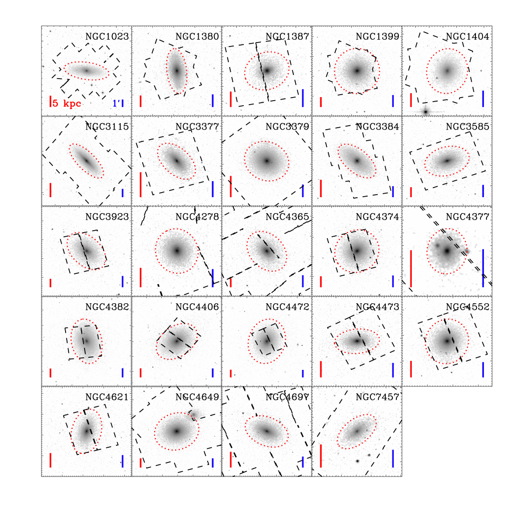
Figure 1: Log-scale 2MASS $K_{\_}s$-band images of the 24 galaxies in our sample. All images have square dimensions with the length of each side being equal to two times the $K_{\_}s$-band major axis corresponding to $\approx$20 mag arcsec^-2 (as reported by Jarrett et al. 2003). The galactic regions are highlighted with red dotted ellipses, and the HST ACS coverage of each galaxy has been shown with dashed polygonal regions. Note that some of the ACS regions are complex (e.g., NGC 4278 and NGC 4365) due to chip gaps. For reference, vertical bars of size 5 kpc and 1 arcmin are provided in the lower-left (red) and lower-right (blue) of each panel, respectively.

2 Sample Selection and Properties

We began by selecting a sample of relatively nearby ($D\lower 2.15277pt\hbox{$\;\buildrel<\over{\sim}\;$}25$ Mpc) early-type galaxies (from E to S0 morphologies across the Hubble sequence) that had available deep Chandra ACIS ($\;\buildrel>\over{\sim}\;$40 ks depth) data, as well as HST ACS imaging over two bandpasses in the optical/near-IR (see Section 3.2 below). These requirements allow us to identify X-ray point-sources, isolate the faint optical counterparts, and effectively classify these counterparts as GC or unrelated foreground/background objects (e.g., Galactic stars and active galactic nuclei [AGN]). We also required that the galaxies have estimates of the GC richness, via measurements of the GC specific frequency, $S_{\_}N$ (see Section 1).

We chose to make use of the Harris et al. (2013; hereafter, H13) catalog of 422 galaxies with published measurements of GC population properties. The H13 catalog consists of culled results, including values of $S_{\_}N$, from 112 papers that had been published before 2012 December. We note that the HST data for our sample is excellent for detecting and characterizing GCs and computing $S_{\_}N$; however, the HST footprints of these data are often constrained to regions that do not encompass the full extents of the GC populations. In this study, we are interested in characterizing GC-related LMXB populations that are directly associated with GCs, as well as those ejected by GCs that are observed in galactic fields. For many galaxies in our sample, the latter “seeded” LMXB populations are expected to have contributions from GCs located well outside of the observational fields. As such, we make use of “local” specific frequencies, $S_{\_}{N,{\rm loc}}$, which we calculate using the HST data presented here (see Section 3.2), when studying LMXB populations directly associated with GCs. We also make use of the “global” $S_{\_}N$ values derived from H13 when studying seeded LMXB populations.

Using the criteria above, and rejecting galaxies that were very close to edge-on (e.g., NGC 5866), had significant dust lanes (e.g., NGC 4526), or had widely variable data coverage across the extents of the galaxies (e.g., M87 and Cen A), we identified 24 elliptical galaxies from the H13 sample that were suitable for our study. These galaxies and their properties are tabulated in Table 1. In Figure 1, we show Two Micron All Sky Survey (2MASS) $K_{\_}s$-band image cutouts of the sample. Our sample spans the full morphological range of our initial selection (E to S0). The majority of the galaxies are in groups or cluster environments, including three members from the M96 group, four Fornax cluster galaxies, and eight Virgo cluster galaxies. Our sample spans a galactic stellar mass range of $\log M_{\_}\star=$ 9.7–11.1, with a median $\log M_{\_}\star^{\rm med}=$ 10.6. The GC specific frequency range is broad, spanning $S_{\_}N=$ 0.6–9.3, with a median value of $S_{\_}N^{\rm med}=$ 2.0. As such, this sample is GC rich compared to similar mass late-type galaxies, which have a median $S_{\_}N\approx 1$ (H13).

Given that our sample is selected from the complex combination of availability of GC property measurements from the literature (as per H13) and the existence of Chandra and HST data, we do not regard this sample as representative of any specific early-type galaxy population. For instance, the selection bias of the sample favors massive early-type galaxies with rich GC systems (see, e.g., Brodie & Strader 2006). Despite the heterogeneous selection, our approach here is to quantify how the XRB population XLFs in these galaxies are correlated with host-galaxy properties and to assess how well these trends describe all of the galaxies individually. If such a “global” model is successful for all galaxies, it is likely (though not guaranteed) to be applicable to other galaxies with similar morphologies, mass ranges, and GC $S_{\_}N$ ranges. However, lower-mass early-type galaxies and galaxies with different morphological types (e.g., late-type galaxies) can often have different star-formation histories, GC $S_{\_}N$ values, and metallicities that can have an effect on the XRB populations (see, e.g., Fragos et al. 2008, 2013a, 2013b; Basu-Zych et al. 2013, 2016; Brorby et al. 2016; Lehmer et al. 2014, 2019; Fornasini et al. 2019).

3 Data Analysis

To address the goal of quantifying how the field LMXB XLF is influenced by stellar ages and the injection of sources that originate in GCs, we require knowledge of (1) the star-formation histories (SFHs) of the galaxies, (2) the GC source locations, and (3) the X-ray source locations. As such, we calculate coarse SFHs using spectral energy distribution (SED) fitting procedures applied to FUV–to–FIR data sets, directly identify GCs in our galaxy sample using HST imaging data, and identify X-ray point sources using Chandra data. Our data analysis procedures and results are detailed below.

Table 2: Multiwavelength Coverage Used in SED Fitting

	GALEX		Swift
Galaxy
(NGC)	FUV	NUV	UVW2	UVM2	UVW1	$U$	$B$	$V$
1023	$-0.25\pm 0.06$	$0.36\pm 0.06$	$\ldots$	$\ldots$	$\ldots$	$\ldots$	$\ldots$	$\ldots$
1380	$-0.20\pm 0.06$	$0.15\pm 0.06$	$0.18\pm 0.02$	$0.14\pm 0.02$	$0.65\pm 0.02$	$1.29\pm 0.02$	$\ldots$	$\ldots$
1387	$-0.28\pm 0.06$	$0.10\pm 0.06$	$\ldots$	$\ldots$	$\ldots$	$\ldots$	$\ldots$	$\ldots$
1399	$0.33\pm 0.06$	$0.49\pm 0.06$	$0.57\pm 0.02$	$0.51\pm 0.02$	$0.90\pm 0.02$	$1.50\pm 0.02$	$2.05\pm 0.02$	$2.39\pm 0.02$
1404	$-1.21\pm 0.07$	$-0.23\pm 0.06$	$0.69\pm 0.02$	$0.64\pm 0.02$	$1.22\pm 0.02$	$1.79\pm 0.02$	$2.36\pm 0.02$	$2.69\pm 0.02$

NOTE.—All columns, with the exception of the first column, provide the logarithm of the flux, with 1$\sigma$ error, for each of the noted bandpass. The fluxes are quoted in units of mJy and are appropriate for the regions described in Section 3.1. Only a portion of the table is shown here to illustrate form and content. The full table is available in machine-readable form and provides flux measurements for all 24 galaxies and 31 different bandpasses.

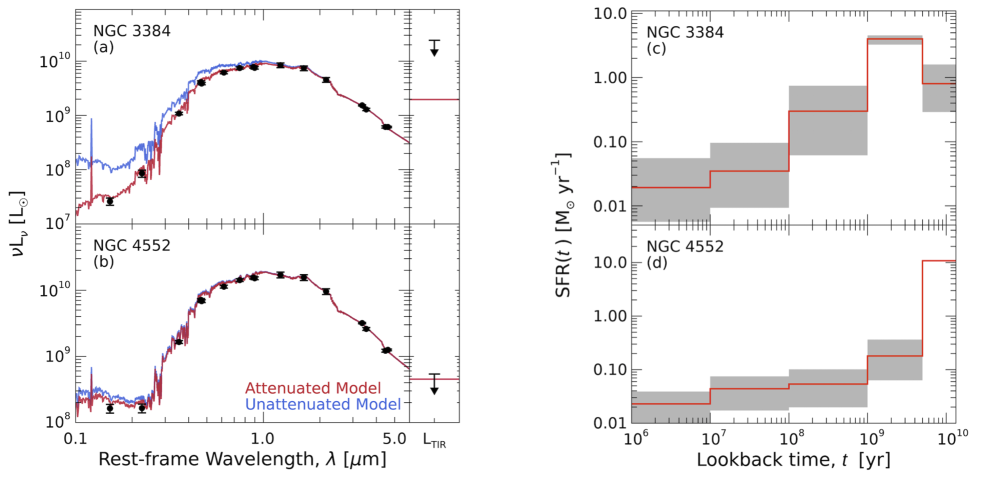
Figure 2: (Left) The observed UV–to–IR SED and the integrated total infrared (TIR) luminosity using the 24$\mu$m-based calibration from Galametz et al. (2013) are shown for NGC 3384 ($a$) and NGC 4552 ($b$), the galaxies with the respectively youngest and oldest stellar-mass weighted ages in our sample. For each galaxy, the best-fit model and unattenuated, intrinsic model are shown as the red and blue curves, respectively. (Right) The resulting SFHs (median values) and 16–84% uncertainty ranges on the SFHs (gray shaded regions) for NGC 3384 ($c$) and NGC 4552 ($d$). The SFHs of all the galaxies in our sample strongly favor large contributions from old stellar populations, and have mass-weighted stellar ages ranging from $\approx$4–9 Gyr, bracketed by the galaxies displayed here. A full version of this figure for all 24 galaxies in our sample can be found in the electronic version.

3.1 FUV to FIR Data Reduction and Star-Formation History Estimates

The FUV–to–FIR SEDs for all 24 galaxies were extracted using publicly available data from GALEX, Swift, HST, SDSS, 2MASS, WISE, Spitzer, and Herschel. For a given galaxy, we limited our analyses to regions that consisted of the intersection of the galactic extent, as estimated by an ellipse approximating the 2MASS $K_{\_}{s}$-band $\approx$20 mag arcsec^-2 isophotal contour (from Jarrett et al. 2003), and the HST coverage of the galaxy (see Section 3.2 below). These regions (the galactic ellipses and HST coverage areas) trace the bulk of the stellar mass of the galaxies, while permitting us to directly identify GC and background-source counterparts. Figure 1 highlights these areas for each galaxy and Table 1 provides their sizes and orientations. After visually inspecting HST and Chandra images of the galaxies, we chose to further exclude small, circular regions with 3 arcsec radii from the center of each galaxy to avoid complications from potential AGN or extreme crowding of sources. We note that all 24 galaxies harbor X-ray detected sources within these nuclear regions, with NGC 1380, NGC 1399, NGC 1404, NGC 3923, NGC 4278, NGC 4365, NGC 4374, NGC 4552, and NGC 4649 containing sources in these regions with 0.5–8 keV luminosities in the range of (1–20) $\times 10^{39}$ erg s^-1. Such sources are not highly luminous AGN, but are strong candidates for low-luminosity AGN. When constructing our SEDs, we extracted photometry from regions that were within the ellipses that had HST exposure, yet were outside the central excluded core. As such, these properties are not representative of the entire galaxy, but in most cases are a significant fraction of the total stellar mass. Hereafter, all quoted properties, with the exception of $S_{\_}N$, are derived from these regions.

For each imaging data set from GALEX FUV to WISE 4.6 $\mu$m, we masked full width at half maximum (FWHM) circular regions at the locations of all foreground Galactic stars that were within the galactic extents defined above and replaced the photometry with local median backgrounds, following the procedure described in Section 2.2 of Eufrasio et al. (2017). We assumed that the contribution from foreground stars at $\;\buildrel>\over{\sim}\;$5 $\mu$m is negligible. Once foreground stars were removed and replaced, the total photometry of the coverage region for each band was calculated by summing all pixels within the region after the diffuse background emission was subtracted. Uncertainties were determined from a combination of background and calibration uncertainties using the methods described in Eufrasio et al. (2014). If a band had incomplete coverage within the galactic extents, or if its total photometry was less than 3$\sigma$ above the background level, that band was excluded from our SED fitting analysis. In Table 2, we summarize the bands that satisfied the above criteria for each galaxy and were used in our SED fitting.

To fit a given SED and estimate the corresponding SFH, we used the Lightning SED fitting code (Eufrasio et al. 2017). Lightning is a non-parametric SED fitting procedure, which fits the stellar emission from the FUV to the NIR (through WISE 4.6$\mu$m), including extinction that is restricted to be in energy balance with the dust emission in the FIR (WISE 22$\mu$m to Herschel 250$\mu$m). The stellar SED is based on the PÉGASE (Fioc & Rocca-Volmerange 1997) population synthesis models and a SFH model that consists of five discrete time steps, of constant SFR, at 0–10 Myr, 10–100 Myr, 0.1–1 Gyr, 1–5 Gyr, and 5–13.3 Gyr. The stellar emission from these specific age bins provide comparable bolometric contributions to the SED of a typical late-type galaxy SFH, and contain discriminating features that can be discerned in broad-band SED fitting (see Eufrasio et al. 2017 for details).

The reprocessed dust emission is modeled as a single measurement of the integrated 8–1000 $\mu$m total infrared luminosity, $L_{\_}{\rm TIR}$, which is estimated based on the Galametz et al. (2013) scaling of 24 $\mu$m Spitzer (or 22$\mu$m from WISE when Spitzer was unavailable) to $L_{\_}{\rm TIR}$. Since elliptical galaxies typically contain low levels of dust emission and little obscuration, the 24 $\mu$m emission can have contributions from stellar emission, as well as dust heated by stellar light from the central region of the galaxy that is masked out (see above). Furthermore, the Galametz et al. (2013) prescription is appropriate for dust heated by young stellar populations, which is likely to overestimate $L_{\_}{\rm TIR}$ (e.g., Temi et al. 2005). As such, we treat our estimates of $L_{\_}{\rm TIR}$ as upper limits, with high-luminosity Gaussian tails with 1$\sigma$ values set equal to the scatter-related uncertainties provided in Table 2 of Galametz et al. (2013).

Figure 2 shows example UV–to–IR SED fit results (including SED models and resulting SFHs from Lightning) for NGC 3384 and NGC 4552, which have, respectively, the youngest and oldest mass-weighted stellar ages in our sample: $4.54\pm 1.07$ Gyr and $9.09\pm 0.05$ Gyr, respectively (see Col.(12) of Table 1). We note that all galaxies, except for NGC 3384, have mass-weighted stellar ages estimated to be in the narrow range of $\;\buildrel>\over{\sim}\;$5 Gyr, with a full-sample mean mass-weighted stellar age of $8.31\pm 0.24$ Gyr (1$\sigma$ error on the mean). All galaxies are fit well by our SED models (fits for all 24 galaxies are provided in the electronic version in an expanded version of Figure 2).

The mass-weighted age range of our sample indicates that our galaxies are expected to have XRB populations dominated by old LMXBs with little diversity in host stellar-population age. This lack of diversity is in contrast to the $\approx$2–15 Gyr stellar age estimate range reported in the literature for these same galaxies (e.g., Trager et al. 2000; Terlevich & Forbes 2001; Thomas et al. 2005; McDermid et al. 2006; Sánchez-Blázquez 2006). However, these other estimates are based primarily on absorption line strength measurements from optical spectra that are appropriate for single or light-weighted age stellar populations. These ages are thus strongly sensitive to metallicity and SFH variations (e.g., Rogers et al. 2010) and can differ in value by as much as a factor of $\approx$4 between studies. Furthermore, mid-IR-based studies have shown that elliptical galaxies with young-age estimates (e.g., $\;\buildrel<\over{\sim}\;$5 Gyr) commonly overpredict the observed IR luminosities, suggesting these galaxies are likely dominated by older ($\;\buildrel>\over{\sim}\;$5 Gyr) stellar populations (e.g., Temi et al. 2005). We calculate from our SFH model SEDs that $B$-band-luminosity-weighted ages are $\approx$0.3–3 Gyr younger than mass-weighted ages. More appropriate to LMXB studies are “mass weighted” stellar ages, which are difficult to derive from optical spectroscopy alone due to low levels of optical emission from old stellar populations. Our SED fitting methods, by contrast, use information from UV, near-IR, and far-IR, which allow for better decomposition of the SFHs of galaxies, with much less sensitivity to metallicity variations, compared to optical spectroscopic line indices. We are therefore confident that our SED fitting results are sufficiently robust for further interpretations throughout this paper.

Table 3: HST Advanced Camera for Surveys (ACS) Observation Log

					Line Dither Pattern
			Exposure Time				Spacing
	Field	Obs. Start	(s)		$N_{\_}{\rm pts}$		(arcsec)
Galaxy	Number	(UT)
(1)	(2)	(3)	(4)	(5)	(6)	(7)	(8)	(9)
			F475W	F850LP	F475W	F850LP	F475W	F850LP
NGC 1023……	1	2011-09-21 00:36	768	1308	2	3	0.145	0.145
	2	2011-09-23 22:44	776	1316	2	2	0.145	0.145
	3	2011-09-21 20:59	768	1308	2	3	0.145	0.145
	6	2011-09-23 00:52	768	1308	2	3	0.145	0.145
	7	2011-09-26 19:14	776	1316	2	2	0.145	0.145
	8	2012-10-14 06:09	768	1308	2	3	0.145	0.145
			F475W	F850LP	F475W	F850LP	F475W	F850LP
NGC 1380……	1	2004-09-06 23:54	760	1220	2	2	0.146	0.146
	2	2006-08-03 23:53	680	…	2	…	2.8	…
			F475W	F850LP	F475W	F850LP	F475W	F850LP
NGC 1387……	1	2004-09-10 14:48	760	1220	2	2	0.146	0.146
			F475W	F850LP	F475W	F850LP	F475W	F850LP
NGC 1399……	2	2004-09-11 07:59	760	1220	2	2	0.146	0.146
	2	2006-08-02 23:54	680	…	2	…	2.8	…

Note.—An abbreviated version of the table is displayed here to illustrate its form and content. Col.(1): Target name. Col.(2): Field number for HST. Col.(3): Observation start. Col(4)–(5): Exposure time for HST filters listed. Col.(6)–(7): Number of points in line dither pattern, $N_{\_}{\rm pts}$, for HST filters listed. Col.(8)–(9): Spacing in arcsec for HST filters listed. Instances with dots denote no data available.
(This table is available in its entirety in machine-readable form.)

3.2 HST Data Reduction

By selection, our galaxies have HST ACS coverage in both “blue” and “red” filters (defined below) and cover the bulk of the stellar mass within the $K_{\_}s$-band ellipses of the galaxies. Figure 1 shows the HST footprints for each of our galaxies and Table 3 provides an observational log of the data sets used. Half of our galaxies (i.e., 12) have HST data covering the full $K_{\_}s$-band ellipses. The remaining twelve galaxies only miss peripheral edges of the $K_{\_}s$ band ellipses (see Fig. 1). For 21 of the galaxies, we used the F475W ($g_{\_}{475}$) and F850LP ($z_{\_}{850}$) bandpasses as our blue and red filters, respectively; however, when this combination was not available, we utilized F475W and F814W ($z_{\_}{814}$) (NGC 1404 and NGC 4382) or F606W ($r_{\_}{606}$) and F814W (NGC 3923) filter pairs.

For each galaxy that had more than one HST field of view, we created mosaicked images. These were constructed by first running the Tweakreg and Tweakback tools (Fruchter & Hook 2002), available in the Drizzlepac version 2.1.14, STScI package. These tools first identify discrete sources that are common to all images in a given overlapping region, and then update the image headers to align with one of the images (chosen as a reference), once an astrometric solution is found. Given the small overlaps between some image sets, we implemented only small linear shifts in right ascension and declination to align our images (typically only a few pixels, but up to 50 pixels in one case). After aligning all ACS fields of both filters for a given galaxy, we then generated the mosaicked blue and red images by running astrodrizzle. The astrodrizzle procedure uses the aligned, flat-field calibrated and charge-transfer efficiency (CTE) corrected images to create a distortion-corrected mosaicked image with bad pixels and cosmic rays removed.

To construct HST source catalogs, we ran SExtractor (Bertin & Arnouts 1996) on each image mosaic. We used a minimum of 10 above-threshold pixels for detection, with detection and analysis thresholds set to 5$\sigma$. We used FWHM 2.5 pixels filtering Gaussians. Two apertures were used for photometry, with radii of $r_{\_}1=0\farcs 31$ (6.25 pixels) and $r_{\_}2=0\farcs 63$ (12.5 pixels). The zeropoints used are from the ACS zeropoint calculator. Gains were calculated using the exposure times and the CCDGAIN header keywords. The background meshes were $8\times 8$ pixels with a background filter size of 2.5 pixels FWHM. We required that sources be present in both filters within a tolerance of 0$\farcs$2 and have FWHM $>$ 1$\farcs$5 to eliminate cosmic ray detections that were not rejected by astrodrizzle (e.g., near image edges and gaps that have dithered exposures).

Table 4: HST Source Classifications and $S_{\_}{N,{\rm loc}}$ Estimates

		Optical				X-ray Detected
Gal	$M_{\_}g^{50}$
(NGC)	(mag)	$N_{\_}{\rm bkg}$	$N_{\_}{\rm GC}$	$M_{\_}{V,{\rm loc}}$	$S_{\_}{N,{\rm loc}}$	$N_{\_}{\rm X}$	$N_{\_}{\rm bkg}$	$N_{\_}{\rm GC}$	$N_{\_}{\rm field}$
(1)	(2)	(3)	(4)	(5)	(6)	(7)	(8)	(9)	(10)
1023	$-$4.9	206	195	$-$20.2	1.65$\pm$0.12	66	3	7	56
1380	$-$6.0	60	293	$-$20.2	3.03$\pm$0.18	35	0	15	20
1387	$-$6.1	281	260	$-$19.8	4.23$\pm$0.26	13	1	8	4
1399	$-$6.2	104	817	$-$20.8	5.09$\pm$0.18	146	8	75	63
1404	$-$6.2	124	233	$-$20.5	1.94$\pm$0.13	62	12	14	36
3115	$-$4.6	211	234	$-$20.2	2.10$\pm$0.14	131	9	32	90
3377	$-$4.9	84	116	$-$18.8	3.60$\pm$0.33	14	0	7	7
3379	$-$4.7	163	97	$-$19.6	1.48$\pm$0.15	86	8	11	67
3384	$-$4.8	78	97	$-$19.4	1.69$\pm$0.17	22	1	1	20
3585	$-$6.3	74	171	$-$21.0	0.95$\pm$0.07	60	2	13	45
3923	…	225	519	$-$20.8	2.45$\pm$0.11	82	3	26	53
4278	$-$5.7	61	346	$-$19.9	4.51$\pm$0.24	146	3	58	85
4365	$-$6.5	75	634	$-$21.1	3.52$\pm$0.14	152	6	60	86
4374	$-$6.0	98	411	$-$21.1	1.97$\pm$0.10	97	2	21	74
4377	$-$5.9	46	54	$-$18.4	2.91$\pm$0.40	4	0	0	4
4382	$-$6.0	176	514	$-$21.1	2.30$\pm$0.10	55	4	13	38
4406	$-$5.8	62	324	$-$20.8	1.80$\pm$0.10	15	1	0	14
4472	$-$5.8	112	617	$-$21.3	2.33$\pm$0.09	200	8	58	134
4473	$-$5.5	72	176	$-$19.6	2.78$\pm$0.21	24	2	5	17
4552	$-$5.6	64	311	$-$20.1	3.15$\pm$0.18	113	4	36	73
4621	$-$5.5	60	242	$-$20.0	2.71$\pm$0.17	37	2	8	27
4649	$-$5.8	519	1054	$-$21.3	3.78$\pm$0.12	286	22	95	169
4697	$-$5.0	99	296	$-$20.1	2.96$\pm$0.17	83	3	32	48
7457	$-$5.2	60	101	$-$18.6	4.05$\pm$0.40	8	0	0	8
Total		3114	8112	…	…	1937	104	595	1238

Note.—Breakdown of the HST-based classifications for discrete optical sources detected within the footprints of the galaxies. In Col.(2), we quote the effective 50% completeness limit for the F475W band ($g_{\_}{475}$), appropriate for sources with GC-like light profiles. In Col.(3) and (4), we include the total numbers of GC and background sources. Col.(5) and (6) provides the “local’ absolute $V$-band magnitudes of the host galaxy and GC specific frequencies, respectively, appropriate for the galactic footprints. In Col.(7)–(10) we list the total number of X-ray detected sources ($N_{\_}{\rm X}$), and the numbers of these sources classified as background sources, GCs, and field populations.

We refined the absolute astrometry of our HST data products and catalogs by aligning them to either the Thirteenth Sloan Digital Sky Survey (SDSS) Data Release (DR13; Albareti et al. 2017) frame or the United States Naval Observatory catalog USNO-B (Monet et al. 2003) frame when SDSS DR13 data were unavailable or inadequate (12 galaxies). In this alignment procedure, HST products were matched to the reference catalogs using small shifts in R.A. and Dec (ranging from 0$\farcs$15–0$\farcs$9). Translational shifts were then applied to the HST images and catalogs to bring them into alignment with the reference catalogs. Based on the distributions of offsets of source matches, we estimate the 1$\sigma$ uncertainties on the image registrations to be in the range of 0$\farcs$04–0$\farcs$3 (median of $\approx$0$\farcs$1).

Using the shifted catalogs, we classified all individually-detected sources that were present within the $K_{\_}s$-band ellipses defined in Table 1. Sources were classified as likely GCs if they had (1) colors in the range of $0.6\leq g_{\_}{475}-z_{\_}{850}\leq 1.6$, $0.5\leq g_{\_}{475}-z_{\_}{814}\leq 1.3$, or $0.3\leq r_{\_}{606}-z_{\_}{814}\leq 0.8$, depending on filter availability; (2) absolute magnitudes (based on the distances to each galaxy) in the range of $-12.5\leq M_{\_}z\leq-6.5$; (3) extended light profiles in either of the blue or red bandpasses, characterized as having SExtractor stellarity parameters CLASS_STAR $\leq$ 0.9 or aperture magnitude differences $m(r_{\_}1)-m(r_{\_}2)>0.4$, where apertures consist of circles with radii $r_{\_}1$ and $r_{\_}2$ (defined above); and (4) light profiles in both the blue and red bands that were not too extended to be GCs, defined as $m(r_{\_}1)-m(r_{\_}2)\leq 0.9$. All other HST-detected sources were classified as unrelated background source candidates (mainly background galaxies and some Galactic stars). Visual inspection of the GC and background sources classified using the above criteria indicates that the misclassification rate is $\approx$1–2%, and is unlikely to have any important impact on our results. In obvious cases where sources were misclassified and are coincident with X-ray detected sources, we manually changed their classifications (see below). However, all other sources were classified using the above criteria.

In Table 4, we summarize the number of GCs and background sources classified within the optical footprints of each galaxy (as defined in Table 1). In Appendix A, we present simulations quantifying our completeness to detecting GC-like sources and provide estimates of the “local” GC specific frequencies, $S_{\_}{N,{\rm loc}}$, for the galaxies. In Table 4, we summarize our completeness findings and GC statistics (including $S_{\_}{N,{\rm loc}}$ values) for the galactic regions. Our completeness limits span a range of $-6.3\leq M_{\_}g^{50}\leq-4.7$, which is always fainter than the peak of the GC luminosity functions at $M_{\_}g\approx-7.1$ mag (e.g., Harris 2001; Kundu & Whitmore 2001), allowing us to constrain well the GC luminosity function and $S_{\_}{N,{\rm loc}}$.

We find that the values of $S_{\_}{N,{\rm loc}}$ span 0.95–5.09 and are well correlated with the global $S_{\_}N$ values. As expected, the values of the local $V$-band luminosities of our galaxy footprints are lower than the global values reported by H13, with $M_{\_}{V,{\rm loc}}-M_{\_}{V,{\rm H13}}\approx$0.2–1.6 mag (median of 1.1 mag). Also, our estimated local numbers of GCs are smaller than the global values provided by H13, with the exception of NGC 4649, in which we estimate a $\approx$38% larger number of GCs within our field of view. Upon detailed inspection, we found that the value quoted in H13 for NGC 4649 was taken directly from Jordán et al. (2005), and is appropriate for the number of GCs within the half-light radius and not the total number of GCs quoted by H13 for other galaxies. As such, the global $S_{\_}N$ value inferred for this source would be underestimated. We therefore estimated the global $S_{\_}N$ for NGC 4649 here by applying a correction factor based on the average ratio of $S_{\_}N/S_{\_}{N,{\rm loc}}=1.02\pm 0.77$, determined from the remaining 23 galaxies. The resulting $S_{\_}N$ value and its propagated uncertainty are quoted in Table 1 for NGC 4649, and are used for the remainder of this study.

In general, the relative galactic-light and GC-location profiles for our galaxies show variations in the comparative values of $S_{\_}{N,{\rm loc}}$ and global $S_{\_}N$. For the galactic regions used in this study, we find that $S_{\_}{N,{\rm loc}}$ tends to have somewhat larger (smaller) values compared to $S_{\_}N$, for $S_{\_}N\lower 2.15277pt\hbox{$\;\buildrel<\over{\sim}\;$}3$ ($S_{\_}N\lower 2.15277pt\hbox{$\;\buildrel>\over{\sim}\;$}3$). This trend appears to be driven primarily by the differences between local and global numbers of GCs varying with $S_{\_}N$. At low-$S_{\_}N$, the global and local numbers of GCs are comparable, but as $S_{\_}N$ increases, the numbers of GCs are relatively small locally compared to the global values. Meanwhile, there are no strong trends in differences of $M_{\_}{V,{\rm loc}}$ and $M_{\_}{V,{\rm H13}}$ with $S_{\_}N$.

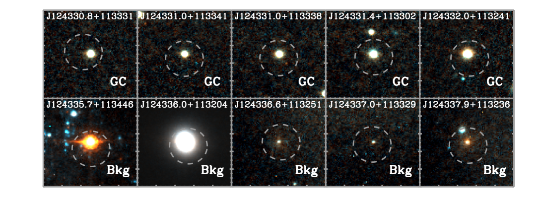
Figure 3: Sample ACS image cutouts for X-ray detected GCs (top panels) and background sources (bottom panels) in NGC 4469. Our optical source counterpart classification criteria are described in Section 3.2. Each postage stamp is centered on the optical source position and spans a $2\farcs 5\times 2\farcs 5$ region. For scaling purposes, we have included a circle with 1^′′ radius centered on the location of the X-ray source.

3.3 Chandra Data Reduction and X-ray Catalog Production

We made use of Chandra ACIS-S and ACIS-I data sets that had aim points within 5 arcmin of the central coordinates of the galaxy (given in Table 1). The observation logs for all galaxies are presented in Table 5. In total 113 unique ObsIDs were used for the 24 galaxies in our sample, representing 5.5 Ms of Chandra observation time. The cumulative exposures ranged from 20–1127 ks, with the deepest observation reaching a minimum 50% completeness limit of $\approx$$10^{36}$ erg s^-1 ($f_{\_}{\rm 0.5-8~{}keV}\approx 10^{-16}$ erg cm^-2 s^-1) for NGC 3115 (Lin et al. 2015).

Our Chandra data reduction and cataloging procedures follow directly the methods used in Sections 3.2 and 3.3 in Lehmer et al. (2019; hereafter, L19). Briefly, for a given galaxy, we performed data reductions of all ObsIDs (updated calibrations, flagged bad pixels, and removed flared intervals), astrometrically aligned ObsIDs to the longest-exposure observation (see Table 5), merged events lists, created images, and searched for point sources using the 0.5–7 keV images for source detection purposes.

Point source and background properties were extracted and computed using the ACIS Extract (AE) v. 2016sep22 software package (Broos et al. 2010, 2012), which calculates point-spread functions (PSFs) from each ObsID, properly disentangles source event contributions from sources with overlapping PSFs, and performs X-ray spectral modeling of each source individually using xspec v. 12.9.1 (Arnaud 1996). As such, all X-ray point-source fluxes are based on basic spectral fits to data using an absorbed power-law model with both a fixed component of Galactic absorption and a free variable intrinsic absorption component (TBABS $\times$ TBABS $\times$ POW in xspec). Throughout the remainder of this paper, we quote point-source X-ray luminosities, $L$, based on the Galactic column-density corrected 0.5–8 keV flux. Following past studies, we do not attempt to correct for intrinsic absorption of the sources themselves.

Table 5: Chandra Advanced CCD Imaging Spectrometer (ACIS) Observation Log

	Aim Point		Obs. Start	Exposurea	Flaringb	$\Delta\alpha$	$\Delta\delta$	Obs.
Obs. ID	$\alpha_{\_}{\rm J2000}$	$\delta_{\_}{\rm J2000}$	(UT)	(ks)	Intervals	(arcsec)	(arcsec)	Modec
NGC1023
4696	02 40 24.87	+39 03 14.72	2004-02-27T18:26:26	10	…	$-$0.04	$-$0.01	V
8197	02 40 22.56	+39 02 03.64	2007-12-12T11:56:14	48	…	$+$0.10	$+$0.15	V
8198d	02 40 22.53	+39 02 34.56	2006-12-17T19:15:53	50	…	…	…	V
8464	02 40 23.53	+39 05 02.70	2007-06-25T17:54:05	48	…	$-$0.31	$+$0.19	V
8465	02 40 14.17	+39 04 59.23	2007-10-15T09:09:05	45	…	$-$0.09	$+$0.19	V
Mergede	02 40 21.01	+39 03 37.09		201	…	…	…	…
NGC1380
9526d	03 36 25.01	$-$34 59 43.63	2008-03-26T12:08:51	41	1, 0.5	…	…	V
NGC1387
4168d	03 36 58.70	$-$35 29 30.78	2003-05-20T22:56:28	46	…	…	…	V

Note.—The full version of this table contains entries for all 24 galaxies and 113 ObsIDs, and is available in machine-readable form. An abbreviated version of the table is displayed here to illustrate its form and content.
^a All observations were continuous. The times shown have been corrected for removed data that were affected by high background.
^b Number of flaring intervals and their combined duration in ks. These intervals were rejected from further analyses.
^c The observing mode (F=Faint mode; V=Very Faint mode).
^d Indicates Obs. ID that all other observations are reprojected to for alignment purposes. This Obs. ID was chosen for reprojection as it had the longest initial exposure time, before flaring intervals were removed.
^e Aim point represents exposure-time weighted value.

To align the Chandra catalogs and data products, we matched the Chandra main catalogs of each galaxy to their corresponding astrometry-corrected HST master optical catalogs using a matching radius of 1$\farcs$0. In this exercise, we limited our matching to X-ray sources with more than 20 0.5–8 keV net counts to ensure reasonable Chandra-derived positions. Most galaxies had respectably large numbers of matches ($\;\buildrel>\over{\sim}\;$15 matches) and showed obvious clusterings of points in $\delta$R. A. and $\delta$dec diagrams, indicating that a reliable astrometric registration could be obtained between Chandra and HST. For these galaxies, we applied additional simple median shifts in R.A. and dec. (offsets ranged from 0$\farcs$08–0$\farcs$66 for the galaxies) to the Chandra data products and catalogs to bring them into alignment with the HST and reference optical frames (by extension). For these galaxies, the final HST and Chandra image and catalog registrations have a 1$\sigma$ error of $\;\buildrel<\over{\sim}\;$0$\farcs$25. For the four galaxies (NGC 3384, 4125, 4377, and 4406) where the number of matches was too small ($<$3) to reliably calculate cross-band offsets, we did not apply astrometric shifts to the data. For these galaxies, we estimate, based on the offsets of other galaxies, that the cross-band registration error is $\;\buildrel<\over{\sim}\;$0$\farcs$3.

After applying shifts to the Chandra catalogs and data products, we performed a second round of matching with the HST catalogs to identify reliable counterparts to the X-ray sources. We ran simulations, in which we shifted the X-ray source locations by 5 arcsec in random directions and re-matched to the HST source catalogs, using a variety of source matching radii, to determine the false-match rate. From these simulations, we found that the number of matches as a function of matching radius has a sharp peak around 0$\farcs$1 and declines rapidly with increasing radius. We estimate that beyond a matching radius of $\;\buildrel>\over{\sim}\;$0$\farcs$5, the number of new matches (compared to smaller matching radii) is equivalent to the expected number of false matches. We therefore chose to utilize a matching radius of 0$\farcs$5 when identifying reliable counterparts. From the above analysis, the false-match rate is calculated to be 4–6% for this adopted limit. We note that this estimate is likely to be an overestimate, due to the inclusion of large numbers of sources that are truly associated with optical counterparts (see, e.g., Broos et al. 2011). Figure 3 shows HST cutout images for a random selection of X-ray sources with GC and background counterparts for the galaxy NGC 4649.

In Appendix B, we present the properties of all 3923 point sources detected in the 0.5–7 keV band within the Chandra images, and include, when possible, HST source classifications. Throughout the remainder of this paper, we focus our analyses on the 1937 sources within the galactic footprints defined above (i.e., within the $K_{\_}s\approx 20$ mag arcsec^-2 ellipses, in areas with HST coverage, and outside of the central removed regions). In Table 4, we summarize for each galaxy the number of these Chandra sources with HST counterparts among the three source categories defined above: i.e., background sources, GC, or field LMXB candidate (when no counterpart is present). In total, 104, 595, and 1238 sources are classified as background sources, GCs, and field LMXB candidates, respectively.

As we will describe below, our results rely on our GC LMXB designations being highly complete, and not having a large number of field LMXBs that could be associated with faint GCs below our optical detection thresholds. In Appendix A, we address this in detail and show that our procedures are capable of recovering the GC-LMXB designation for $\approx$96% of the GC-LMXBs that are among our X-ray detected sources. As such, our field LMXB population will contain at most a negligible population of faint GCs that are simply undetected.

4 Results

Our XLF fitting procedures followed the same techniques developed and presented in Section 4.1 of L19; the salient details of this procedure are provided below. All XLF data are fit using a forward-fitting approach, in which detection incompleteness, contributions from cosmic X-ray background (CXB) sources (hereafter, defined as unrelated Galactic stars and background AGN or normal galaxies), and LMXB model components are folded into our models to fit observed XLFs. On occasion, we display completeness-corrected and CXB-subtracted XLFs for illustrative purposes, but do not use such data in our fitting. Below, we describe the construction of the model components and present our fitting results.

4.1 Cosmic X-ray Background Modeling

Many of the CXB sources can be directly classified using our HST data; however, our ability to accurately classify X-ray detected background objects depends on the HST imaging depth. In practice, there will be a number of X-ray detected CXB sources that have no HST counterparts that we will classify here as LMXB candidates. Even in blank-field extragalactic X-ray surveys with very deep extensive multiwavelength follow-up (e.g., Nandra et al. 2015; Civano et al. 2016; Xue et al. 2016; Luo et al. 2017; Kocevski et al. 2018), there are a number of X-ray sources with no multiwavelength counterparts. The CXB sources will be dominated by AGN that have optical fluxes that broadly correlate with X-ray flux, so the most likely sources to lack HST counterpart identifications are those with the faintest X-ray fluxes. We assessed the level of completeness by which we could reliably identify CXB source counterparts by comparing the expected extragalactic number counts from blank-field surveys with our background-object counts.

In Figure 4, we show the number of background sources detected as a function of 0.5–8 keV flux, $S$, compared to the expected number from the extragalactic number counts from Kim et al. (2007). Note that the extragalactic number counts curve has been corrected for X-ray incompleteness of our data sets at faint limits (see L19 for details).

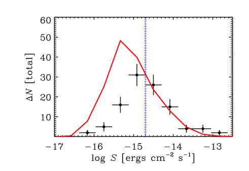
Figure 4: Observed number of sources $\Delta N$ per flux bin ($\Delta\log S=0.42$ dex) classified as CXB sources as a function of 0.5–8 keV flux $S$ for all galaxies combined. In total, 104 sources were classified as background sources. The predicted number of background objects for the full sample is shown as a solid red curve (based on the Kim et al. 2007 extragalactic number counts). This prediction is based on the extragalactic number counts, and includes the effects of incompleteness. We find that our background counts are consistent with the extragalactic counts above $S>2\times 10^{-15}$ erg cm^-2 s^-1 (blue dotted line), but become highly incomplete ($\;\buildrel<\over{\sim}\;$10–50%) below this flux level. In our XLF fitting, we directly excluded CXB sources above this flux level, and modeled the contributions from fainter sources using the Kim et al. (2007) results.

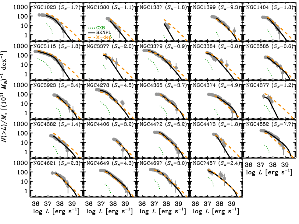
Figure 5: Observed field LMXB XLFs for all galaxies in our sample (gray circles with 1$\sigma$ error bars). Each panel provides the XLF of the denoted galaxy and includes the GC specific frequency value, $S_{\_}N$, for convenient reference. These XLFs have been constructed by excluding all X-ray sources designated as GCs, but include potential background sources. They are not corrected for incompleteness, explaining the perceptible turnovers at the lowest luminosity values. Model fits, which include contributions from the CXB (green dotted curves) and intrinsic point sources, are shown for the broken power-law model (black solid curves) and the global stellar-mass dependent model (dashed orange curves). Displayed models (and CXB contributions) include the effects of incompleteness, and are calculated down to the 50% completeness limit $L_{\_}{50}$. As described in Section 4.1, directly identified background sources with 0.5–8 keV fluxes $S\lower 2.15277pt\hbox{$\;\buildrel>\over{\sim}\;$}2\times 10^{-15}$ erg cm^-2 s^-1 have been removed, so our CXB model only includes contributions from sources with $S<2\times 10^{-15}$ erg cm^-2 s^-1 (or $L=$ 2.5–13 $\times 10^{37}$ erg s^-1, depending on the galaxy).

We find that the observed CXB number counts for our sample match well the expected number counts for $S\lower 2.15277pt\hbox{$\;\buildrel>\over{\sim}\;$}2\times 10^{-15}$ erg cm^-2 s^-1, suggesting that our background source identification methods are reliable and highly complete above this limit. However, for sources below this limit, our observed source counts are below the predictions by a significant margin ($\approx$10–50% complete), indicating there are some CXB sources in this regime that we are likely misclassifying as field LMXB candidates. Given these results, hereafter we chose to reject from our field LMXB XLF analyses all CXB sources with $S\geq 2\times 10^{-15}$ erg cm^-2 s^-1 (corresponding to $L\approx$ 2.5–13 $\times 10^{37}$ erg s^-1 for our sample), but include all background sources fainter than this limit. We account for these faint CXB sources when modeling the XLFs by implementing the Kim et al. (2007) extragalactic number counts at $S<2\times 10^{-15}$ erg cm^-2 s^-1.

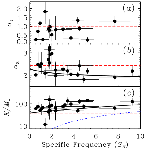
Figure 6: ($a$)–($c$): Best-fitting broken power-law parameters for field LMXB populations for each galaxy versus GC specific frequency. We include here the ($a$) low-luminosity XLF slope ($L<L_{\_}b$; $L_{\_}b=3\times 10^{37}$ erg s^-1) for galaxies with $L_{\_}{50}<L_{\_}b$, as well as ($b$) high-luminosity XLF slope ($L>L_{\_}b$) for galaxies with $L_{\_}{50}<10^{38}$ erg s^-1, and ($c$) stellar-mass scaled XLF normalization for all galaxies. The predicted trends from our best-fit in-situ and GC-seeded model of field LMXBs (discussed in Section 4.5) are shown for in-situ LMXBs (red long-dashed lines), GC-seeded LMXBs (blue short-dashed curves), and combined populations (black solid cuves).

4.2 Field LMXB X-ray Luminosity Functions By Galaxy

We started by characterizing the field LMXB XLFs of each galaxy using basic analytic models (i.e., power-law and broken power-law). Since our focus here is on the field LMXBs, we rejected all X-ray sources coincident with GCs and the subset of known CXB sources with $S>2\times 10^{-15}$ erg cm^-2 s^-1(see previous section).

In Figure 5, we show the observed stellar-mass-normalized field LMXB XLFs (in cumulative form) for each of the 24 galaxies in our sample. Note that the data displayed in Figure 5 have not been corrected for incompleteness and therefore do not convey the intrinsic shapes of the XLFs. Following L19, we attempted to model the XLFs of each galaxy using both power-law and broken power-law models:

$$\frac{dN}{dL}=K_{\_}{\rm PL}\left\{\begin{array}[]{lr}L^{-\alpha},&\;\;\;\;\;\;\;\;(L<L_{\_}c)\\ 0,&(L\geq L_{\_}c)\end{array}\right.$$ (1)

$$\frac{dN}{dL}=K_{\_}{\rm BKNPL}\left\{\begin{array}[]{lr}L^{-\alpha_{\_}1}&\;\;\;\;\;\;\;\;(L<L_{\_}b)\\ L_{\_}b^{\alpha_{\_}2-\alpha_{\_}1}L^{-\alpha_{\_}2},&(L_{\_}b\leq L<L_{\_}c)\\ 0,&(L\geq L_{\_}c)\\ \end{array}\right.$$ (2)

where $K_{\_}{\rm PL}$ and $\alpha$ are the single power-law normalization and slope, respectively, and $K_{\_}{\rm BKNPL}$, $\alpha_{\_}1$, $L_{\_}b$, and $\alpha_{\_}2$ are the broken power-law normalization, low-luminosity slope, break luminosity, and high-luminosity slope, respectively; both XLF models are truncated above, $L_{\_}c$, the cut-off luminosity. To make the normalization values more intuitive, we take $L$, $L_{\_}b$, and $L_{\_}c$ to be in units of $10^{38}$ erg s^-1 when using eqns. (1) and (2). For a given galaxy, we fit the data to determine all constants, except for the break and cut-off luminosities, which we fixed at $L_{\_}b=3\times 10^{37}$ erg s^-1 and $L_{\_}c=3\times 10^{39}$ erg s^-1. Also, when the luminosity of the 50% completeness limit, $L_{\_}{50}$, was in the range of 1–2 $\times L_{\_}b$, the fit to $\alpha_{\_}1$ was deemed unreliable, and was fixed to $\alpha_{\_}1=1.0$. For one galaxy, NGC 4406, $L_{\_}{50}>10^{38}$ erg s^-1, and we chose to fix $\alpha_{\_}1=1.0$ and $\alpha_{\_}2=2.1$ and fit only for the normalization. The above specific choices for fixed parameter values were motivated by global fits to the full sample (see Section 4.3).

Following the procedures in L19, we modeled the observed XLF, $dN/dL({\rm obs})$, using the intrinsic power-law and broken power-law model of the XRB XLF, $dN/dL({\rm int})$, plus an estimated contribution from undetected background sources, $dN/dL({\rm CXB})$, that were convolved with a luminosity-dependent completeness function, $\xi(L)$ (see L19 for details on the calculation of $\xi$):

$$dN/dL({\rm obs})=\xi(L)[dN/dL({\rm int})+dN/dL({\rm CXB})].$$ (3)

For each galaxy, we constructed the observed $dN/dL({\rm obs})$ using luminosity bins of constant $\delta\log L=0.057$ dex that spanned the range of $L_{\_}{\rm min}=L_{\_}{50}$ (the 50% completeness limit) to $L_{\_}{\rm max}=5\times 10^{41}$ erg s^-1. We note that the size of these bins is chosen to be comparable to distance-related uncertainties on the luminosities. For most galaxies, the majority of the bins contained zero sources, with other bins containing small numbers of sources. Therefore, when assessing maximum likelihood we made use of a modified version of the $C$ statistic (cstat; Cash 1979; Kaastra 2017):

$$C=2\sum_{\_}{i=1}^{n}M_{\_}i-N_{\_}i+N_{\_}i\ln(N_{\_}i/M_{\_}i),$$ (4)

where the summation takes place over the $n$ bins of X-ray luminosity, and $N_{\_}i$ and $M_{\_}i$ are the observed and model counts in each bin. We note that when $N_{\_}i=0$, $N_{\_}i\ln(N_{\_}i/M_{\_}i)=0$, and when $M_{\_}i=0$ (e.g., beyond a cut-off luminosity), the entire $i$th term in the summation is zero.

Table 6: Field X-ray Luminosity Function Fits By Galaxy

Galaxy				Single Power Law†				Broken Power Law‡
Name		$\log L_{\_}{50}$	$\log L_{\_}{90}$										$\log L_{\_}{\rm X}$
(NGC)	$N_{\_}{\rm src}$	(erg s-1)	(erg s-1)	$K_{\_}{\rm PL}$	$\alpha$	$C$	$P_{\_}{\rm Null}$	$K_{\_}{\rm BKNPL}$	$\alpha_{\_}1$	$\alpha_{\_}2$	$C$	$P_{\_}{\rm Null}$	(ergs s-1)
(1)	(2)	(3)	(4)	(5)	(6)	(7)	(8)	(9)	(10)	(11)	(12)	(13)	(14)
1023	56	36.8	37.0	7.94${}^{+2.19}_{\_}{-1.83}$	1.35$\pm$0.15	22	0.165	19.7${}^{+7.3}_{\_}{-5.9}$	0.86${}^{+0.23}_{\_}{-0.22}$	2.70${}^{+0.40}_{\_}{-0.34}$	23	0.174	39.5$\pm$0.1
1380	20	37.7	37.8	7.47${}^{+2.60}_{\_}{-2.15}$	1.88${}^{+0.45}_{\_}{-0.49}$	6	0.005	23.6${}^{+12.9}_{\_}{-10.3}$	0.63${}^{+1.07}_{\_}{-0.43}$	2.51${}^{+0.54}_{\_}{-0.45}$	9	0.034	39.7$\pm$0.2
1387	4	37.8	37.9	2.94${}^{+1.81}_{\_}{-1.28}$	2.43${}^{+0.66}_{\_}{-0.58}$	12	0.520	17.4${}^{+18.6}_{\_}{-9.8}$	0.90∗	3.23${}^{+0.96}_{\_}{-0.84}$	13	0.952	39.4$\pm$0.3
1399	66	37.7	38.0	29.2${}^{+4.6}_{\_}{-4.2}$	2.18$\pm$0.16	22	0.034	94.4${}^{+37.2}_{\_}{-28.6}$	0.40${}^{+0.44}_{\_}{-0.25}$	2.19${}^{+0.23}_{\_}{-0.22}$	22	0.171	40.3$\pm$0.1
1404	41	37.5	37.9	11.8${}^{+2.5}_{\_}{-2.2}$	2.30$\pm$0.19	22	0.092	43.1${}^{+18.7}_{\_}{-16.6}$	0.77${}^{+0.62}_{\_}{-0.44}$	2.55${}^{+0.32}_{\_}{-0.28}$	23	0.433	39.9$\pm$0.1
3115	96	36.1	36.4	5.81${}^{+1.12}_{\_}{-0.99}$	1.43$\pm$0.06	53	0.551	20.9${}^{+5.1}_{\_}{-4.3}$	0.97$\pm$0.09	2.92${}^{+0.50}_{\_}{-0.40}$	31	0.156	39.5$\pm$0.1
3377	7	37.2	37.3	1.09${}^{+0.63}_{\_}{-0.45}$	1.90${}^{+0.38}_{\_}{-0.35}$	21	0.973	6.08${}^{+4.54}_{\_}{-3.36}$	0.51${}^{+0.62}_{\_}{-0.36}$	2.96${}^{+0.93}_{\_}{-0.72}$	22	0.250	39.0$\pm$0.2
3379	72	36.4	36.7	5.03${}^{+1.08}_{\_}{-0.99}$	1.56$\pm$0.08	42	0.306	12.8${}^{+4.1}_{\_}{-3.3}$	1.17$\pm$0.13	2.38${}^{+0.36}_{\_}{-0.28}$	36	0.472	39.4$\pm$0.1
3384	21	36.8	36.9	2.13${}^{+0.74}_{\_}{-0.61}$	1.59$\pm$0.17	33	0.729	9.34${}^{+4.99}_{\_}{-3.98}$	0.71${}^{+0.35}_{\_}{-0.30}$	2.48${}^{+0.58}_{\_}{-0.42}$	33	0.759	39.2$\pm$0.2
3585	47	37.5	37.6	14.0${}^{+2.5}_{\_}{-2.3}$	1.84${}^{+0.16}_{\_}{-0.15}$	31	0.465	51.6${}^{+11.7}_{\_}{-10.5}$	0.25${}^{+0.28}_{\_}{-0.16}$	2.01${}^{+0.21}_{\_}{-0.20}$	28	0.464	40.1$\pm$0.1
3923	54	37.7	38.0	26.8${}^{+4.5}_{\_}{-4.1}$	2.19$\pm$0.18	21	0.109	88.5${}^{+34.8}_{\_}{-26.7}$	0.40${}^{+0.37}_{\_}{-0.26}$	2.19${}^{+0.25}_{\_}{-0.22}$	21	0.160	40.2$\pm$0.1
4278	87	36.8	37.3	10.0${}^{+1.7}_{\_}{-1.6}$	1.65$\pm$0.08	54	0.494	37.2${}^{+8.6}_{\_}{-7.4}$	0.87${}^{+0.14}_{\_}{-0.15}$	2.43${}^{+0.25}_{\_}{-0.23}$	39	0.935	39.8$\pm$0.1
4365	89	37.4	37.7	24.1${}^{+3.1}_{\_}{-2.9}$	1.86${}^{+0.11}_{\_}{-0.10}$	35	0.508	91.1${}^{+20.0}_{\_}{-18.2}$	0.33${}^{+0.25}_{\_}{-0.18}$	2.04$\pm$0.15	32	0.522	40.3$\pm$0.1
4374	75	37.5	37.9	21.3${}^{+3.2}_{\_}{-3.1}$	1.74$\pm$0.13	33	0.353	64.6${}^{+14.8}_{\_}{-13.2}$	0.24${}^{+0.28}_{\_}{-0.15}$	1.81${}^{+0.17}_{\_}{-0.16}$	30	0.372	40.3$\pm$0.1
4377	4	37.2	37.5	0.62${}^{+0.52}_{\_}{-0.35}$	1.83${}^{+0.57}_{\_}{-0.48}$	10	0.398	4.82${}^{+4.01}_{\_}{-2.54}$	0.25${}^{+0.40}_{\_}{-0.18}$	3.61${}^{+0.88}_{\_}{-1.05}$	8	0.480	38.8${}^{+0.2}_{\_}{-0.3}$
4382	39	37.4	37.6	9.10${}^{+2.04}_{\_}{-1.81}$	2.03$\pm$0.18	24	0.160	11.4${}^{+8.3}_{\_}{-5.7}$	1.83${}^{+0.70}_{\_}{-0.68}$	2.09${}^{+0.25}_{\_}{-0.24}$	24	0.222	39.8${}^{+0.4}_{\_}{-0.1}$
4406	14	38.2	38.4	82${}^{+146}_{\_}{-49}$	3.30${}^{+1.02}_{\_}{-0.77}$	17	0.991	59.1${}^{+19.7}_{\_}{-15.9}$	0.90∗	2.20∗	16	0.386	40.1$\pm$0.1
4472	138	37.4	37.6	33.7${}^{+3.3}_{\_}{-3.2}$	1.86$\pm$0.08	26	0.007	159.0${}^{+25.8}_{\_}{-23.1}$	0.23${}^{+0.15}_{\_}{-0.13}$	2.18${}^{+0.14}_{\_}{-0.15}$	13	0.002	40.5${}^{+0.0}_{\_}{-0.1}$
4473	17	37.6	37.8	6.33${}^{+2.08}_{\_}{-1.72}$	2.70${}^{+0.41}_{\_}{-0.36}$	15	0.351	32.5${}^{+15.3}_{\_}{-14.1}$	0.59${}^{+0.85}_{\_}{-0.38}$	3.14${}^{+0.60}_{\_}{-0.56}$	15	0.711	39.7${}^{+0.2}_{\_}{-0.1}$
4552	75	37.2	37.7	16.5${}^{+2.4}_{\_}{-2.2}$	1.79$\pm$0.10	34	0.293	28.3${}^{+9.0}_{\_}{-7.4}$	1.29${}^{+0.29}_{\_}{-0.30}$	1.91$\pm$0.15	34	0.417	40.0$\pm$0.1
4621	27	37.6	37.8	11.8${}^{+2.7}_{\_}{-2.5}$	2.18${}^{+0.26}_{\_}{-0.24}$	27	0.907	23.0${}^{+19.5}_{\_}{-15.6}$	1.19${}^{+1.67}_{\_}{-0.77}$	2.23${}^{+0.32}_{\_}{-0.27}$	28	0.812	39.9${}^{+0.8}_{\_}{-0.2}$
4649	180	37.2	37.6	36.4${}^{+3.4}_{\_}{-3.2}$	1.86$\pm$0.07	31	0.109	65.1${}^{+11.8}_{\_}{-11.1}$	1.34$\pm$0.17	2.02${}^{+0.12}_{\_}{-0.10}$	29	0.111	40.3$\pm$0.0
4697	50	36.9	37.1	6.22${}^{+1.39}_{\_}{-1.11}$	1.63${}^{+0.10}_{\_}{-0.11}$	34	0.249	21.7${}^{+7.8}_{\_}{-5.9}$	0.83${}^{+0.22}_{\_}{-0.24}$	2.27${}^{+0.30}_{\_}{-0.25}$	29	0.374	39.6$\pm$0.1
7457	8	37.0	37.2	1.06${}^{+0.58}_{\_}{-0.43}$	1.59$\pm$0.32	19	0.396	2.72${}^{+2.93}_{\_}{-1.57}$	0.80${}^{+0.77}_{\_}{-0.58}$	1.98${}^{+0.63}_{\_}{-0.44}$	21	0.938	38.9$\pm$0.3

Note. — All fits include the effects of incompleteness and model contributions from the CXB, following Eqn. (7). A full description of our model fitting procedure is outlined in Section 4.2. Col.(1): Galaxy NGC name, as reported in Table 1. Col.(2): Total number of X-ray sources detected within the galactic boundaries defined in Table 1. Col.(3) and (4): Logarithm of the luminosities corresponding to the respective 50% and 90% completeness limits. Col.(5) and (6): Median and 1$\sigma$ uncertainty values of the single power-law normalization and slope, respectively – our adopted “best model” consists of the median values. Col.(7): C-statistic, $C$, associated with the best model. Col.(8): Null-hypothesis probability that the best model describes the data. The null-hypothesis probability is calculated following the prescription in Kaastra (2017). Col.(9)–(11): Median and 1$\sigma$ uncertainty values of the broken power-law normalization and slope, respectively. Col.(12) and (13): Respectively, C-statistic and null-hypothesis probability for the best broken power-law model. Col.(14): Integrated X-ray luminosity, $L_{\_}{\rm X}$, for the broken power-law model.

^∗Parameter was fixed due to shallow Chandra depth (see Section 4.2).

^†Single power-law models are derived following Eqn. (1) with a fixed cut-off luminosity of $L_{\_}c=3\times 10^{39}$ erg s^-1.

^‡Broken power-law models are derived following Eqn. (2) with a fixed break luminosity of $L_{\_}b=3\times 10^{37}$ erg s^-1 and cut-off luminosity of $L_{\_}c=3\times 10^{39}$ erg s^-1.

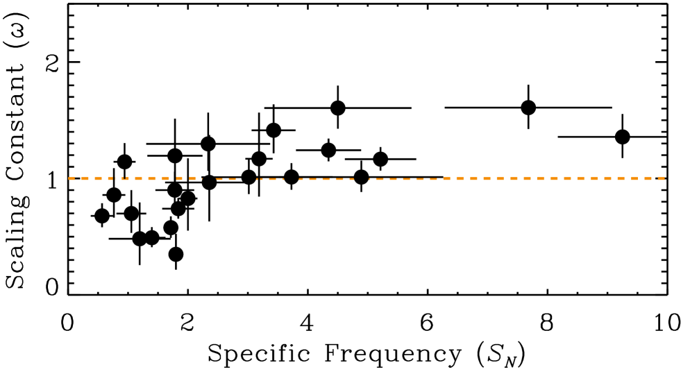
Figure 7: Scaling constant $\omega$, which multiplicatively scales the stellar-mass dependent global XLF model to the XLF of each galaxy, versus $S_{\_}N$ for all 24 galaxies. We find that $\omega$ is correlated with $S_{\_}N$ at the $>99.9\%$ confidence level, indicating field LMXBs are likely seeded by GCs (see Section 4.2 discussion).

4.3 Field LMXB XLF Dependence on Stellar Mass

We calculated parameters, uncertainties, and uncertainty co-dependencies following the Markov Chain Monte Carlo (MCMC) procedure outlined in Section 4.1 of L19. In all fits, we adopted median values of the parameter distributions as our quoted best-fit model parameters and the corresponding $C$ statistic. We find that these values differ only slightly from those derived from the global minimum value of the $C$ statistic. We evaluated the goodness of fit for our model based on the expected $C$-statistic value $C_{\_}{\rm exp}$ and its variance $C_{\_}{\rm var}$, which were calculated following the procedures in Kaastra (2017). The null hypothesis probability for the model was calculated as:

$$P_{\_}{\rm null}=1-{\rm erf}\left(\sqrt{\frac{(C-C_{\_}{\rm exp})^{2}}{2\;C_{\_}{\rm var}}}\right).$$ (5)

In Table 6, we tabulate the best-fit results for our power-law and broken power-law models, including their goodness of fit evaluations. In all cases, the power-law and broken power-law fits result in $P_{\_}{\rm null}>0.001$, with only NGC 1380 and NGC 4472 showing some tension with the models (e.g., $P_{\_}{\rm null}\lower 2.15277pt\hbox{$\;\buildrel<\over{\sim}\;$}0.02$). Figure 5 displays the best-fit broken power-law model for the observed XLFs of each galaxy (black solid curves), along with the model contributions from CXB sources with $S<2\times 10^{-15}$ erg cm^-2 s^-1 (green dotted curves), which in all relevant cases are much lower than the LMXB contributions.

Figure 6 shows the parameters of the broken power-law versus GC $S_{\_}N$. The parameters include faint-end slope $\alpha_{\_}1$, bright-end slope $\alpha_{\_}2$, and normalization per unit stellar mass $K_{\_}{\rm BKNPL}/M_{\_}\star$. Displayed values only include those that were determined via fitting, and exclude parameter values that were fixed as a result of the Chandra data being too shallow. We find suggestive correlations between $\alpha_{\_}2$ and $K_{\_}{\rm BKNPL}/M_{\_}\star$ with $S_{\_}N$; based on Spearman’s rank correlation tests, the correlation is suggestive at the $\approx$97% and $\approx$95% confidence level. This trend suggests that GCs may in fact provide some seeding to the field LMXB population. We explore this more in the sections below.

As discussed in Section 1, several past studies of LMXBs have focused on the scaling of the LMXB XLF with stellar mass; however, very few studies have attempted to isolate this relation for field LMXBs explicitly (however, see Peacock et al. 2017). Here, we determine the shape and scaling of the field LMXB XLF appropriate for our sample as a whole, and subsequently revisit its application to each galaxy in our sample to test for universality. Our stellar-mass dependent XLF can be quantified as:

$$\frac{dN_{\_}M}{dL}=M_{\_}\star\;K_{\_}M\left\{\begin{array}[]{lr}L^{-\alpha_{\_}1}&\;\;\;\;\;\;\;\;(L<L_{\_}b)\\ L_{\_}b^{\alpha_{\_}2-\alpha_{\_}1}L^{-\alpha_{\_}2},&(L_{\_}b\leq L<L_{\_}c)\\ 0,&(L\geq L_{\_}c)\\ \end{array}\right.$$ (6)

where $K_{\_}M$ is the normalization per stellar mass (quoted in units of [$10^{11}$ $M_{\odot}$]^-1) at $L=10^{38}$ erg s^-1, and the remaining quantities have the same meaning as they did in Equation (2). Here we are modeling all data simultaneously, and we can thus allow all the parameters of the fit to be free and directly determine their uncertainties. Thus, we perform fitting for four parameters: $K_{\_}M$, $\alpha_{\_}1$, $L_{\_}b$, and $\alpha_{\_}2$. Due to the steep bright-end slope of the XLF, we are unable to constrain well $L_{\_}c$, and therefore fix its value at $L_{\_}c=10^{40}$ erg s^-1.

Table 7: Summary of Field X-ray Luminosity Function Fits By Galaxy

	Field LMXB XLF
Galaxy	Power Law				$M_{\_}\star$-Dependent		$M_{\_}\star$ and $S_{\_}N$ Dep.		GC XLF		Total XLF
Name	Single		Broken
(NGC)	$C$	$P_{\_}{\rm Null}^{\rm PL}$	$C$	$P_{\_}{\rm Null}^{\rm BKNPL}$	$C$	$P_{\_}{\rm Null}^{M}$	$C$	$P_{\_}{\rm Null}^{\rm field}$	$C$	$P_{\_}{\rm Null}^{\rm GC}$	$C$	$P_{\_}{\rm Null}^{\rm all}$
(1)	(2)	(3)	(4)	(5)	(6)	(7)	(8)	(9)	(10)	(11)	(12)	(13)
1023	22	0.165	23	0.174	52	0.261	43	0.670	36	0.894	51	0.263
1380	6	0.005	9	0.034	17	0.096	15	0.182	32	0.132	36	0.101
1387	12	0.520	13	0.952	27	0.719	21	0.978	23	0.906	22	0.771
1399	22	0.034	22	0.171	41	0.435	43	0.281	56	$<$0.001	47	0.121
1404	22	0.092	23	0.433	30	0.516	28	0.702	24	0.639	28	0.570
3115	53	0.551	31	0.156	47	0.497	40	0.305	43	0.411	49	0.703
3377	21	0.973	22	0.250	23	0.934	22	0.752	17	0.518	25	0.951
3379	42	0.306	36	0.472	47	0.845	52	0.207	33	0.788	56	0.163
3384	33	0.729	33	0.759	36	0.824	35	0.471	13	0.089	32	0.988
3585	31	0.465	28	0.464	45	0.271	39	0.224	27	0.761	37	0.597
3923	21	0.109	21	0.160	28	0.625	27	0.748	36	0.160	32	0.880
4278	54	0.494	39	0.935	62	0.013	54	0.093	42	0.838	64	0.016
4365	35	0.508	32	0.522	41	0.803	38	0.774	36	0.846	37	0.927
4374	33	0.353	30	0.372	46	0.297	41	0.471	23	0.218	44	0.341
4377	10	0.398	8	0.480	15	0.214	13	0.291	…	…	14	0.206
4382	24	0.160	24	0.222	58	0.009	41	0.256	40	0.236	47	0.108
4406	17	0.991	16	0.386	22	0.891	20	0.805	…	…	20	0.937
4472	26	0.007	13	0.002	29	0.097	24	0.064	28	0.399	43	0.962
4473	15	0.351	15	0.711	21	0.646	22	0.838	16	0.269	20	0.448
4552	34	0.293	34	0.417	52	0.048	35	0.744	39	0.461	34	0.613
4621	27	0.907	28	0.812	36	0.165	36	0.063	31	0.220	46	0.005
4649	31	0.109	29	0.111	44	0.943	35	0.588	27	0.250	29	0.201
4697	34	0.249	29	0.374	36	0.765	35	0.855	44	0.181	43	0.679
7457	19	0.396	21	0.938	22	0.873	22	0.995	…	…	22	0.527

Note. — Goodness of fit assessments for all galaxies for the field LMXB population (Col.(2)–(9); Sections 4.2, 4.3, and 4.5), the GC LMXBs (Col.(10)–(11); Section 4.4), and combined field-plus-GC LMXB model (Col.(12)–(13); Section 4.6). Col.(1): Galaxy NGC name, as reported in Table 1. Col.(2)–(5): $C$-statistic and null-hypothesis probability pairs for power-law and broken power-law models of the field LMXBs. These columns are re-tabulations of Col.(7)–(8) and Col.(12)–(13) from Table 6. Col.(6)–(7): $C$-statistic and null-hypothesis probability for the stellar-mass dependent model of the field LMXBs, which is based only on the $M_{\_}\star$ of the galaxy. Col.(8)–(9): $C$-statistic and null-hypothesis probability for the stellar-mass and $S_{\_}N$ dependent model of the field LMXBs. Col.(10)–(11):$C$-statistic and null-hypothesis probability for the GC LMXB population (Eqn. (8)). Col.(12)–(13): $C$-statistic and null-hypothesis probability for the global model, which includes contributions from both field LMXBs and GC LMXBs (see Section 4.6).

When fitting for a global model, like the stellar-mass dependent model, we determine best fit solutions and parameter uncertainties by minimizing the cumulative $C$ statistic:

$$C=\sum_{\_}{i=1}^{n_{\_}{\rm gal}}\left(2\sum_{\_}{j=1}^{n_{\_}{\rm X}}M_{\_}{i,j}-N_{\_}{i,j}+N_{\_}{i,j}\ln(N_{\_}{i,j}/M_{\_}{i,j})\right),$$ (7)

where $C$ is now determined “globally” through the double summation over all $n_{\_}{\rm gal}=$ 24 galaxies ($i$th index) and $n_{\_}{\rm X}=100$ X-ray luminosity bins, spanning $\log L=$ 35–41.7 ($j$th index). Here, the $C$ value for the $i$th galaxy is simply the contribution from the $i$th term of Equation (7) and can be compared with our individual fits from Section 4.2. In total, 1238 X-ray sources were used in the global model fit.

In Figure 5, we show the best-fit stellar-mass dependent global model applied to each of the 24 galaxies as orange dashed curves. The assessed galaxy-by-galaxy null-hypothesis probability, calculated using Equation (5), is tabulated in Table 7 (Col. 7) and the best-fit parameters for the global fit are provided in Table 8. While the stellar-mass dependent global model provides an acceptable fit to the field LMXB data for the majority of the galaxies, there is some tension (e.g., $P_{\_}{\rm null}\lower 2.15277pt\hbox{$\;\buildrel<\over{\sim}\;$}0.02$) in the fits to NGC 4278, NGC 4382, and NGC 4552. Despite these cases, the model is acceptable as globally ($P_{\_}{\rm null}=0.136$).

Visual inspection of Figure 5 suggests that there are no obvious issues with the parameterized shape of the the field LMXB XLF, but instead there is noteworthy variation in the normalizations, with some galaxies having an observed excess of sources (e.g., NGC 1399, NGC 4278, NGC 4472, and NGC 4552) and others having a deficit of sources (e.g., NGC 1380, NGC 1387, NGC 3384, and NGC 4382) compared to the stellar-mass dependent model prediction (orange dashed curves). When considering the GC specific frequencies of these objects, the galaxies with apparent source excesses have high-$S_{\_}N$ and those with apparent deficits have low-$S_{\_}N$.

To test the connection with $S_{\_}N$ further, we re-fit each galaxy XLF using a model with fixed values from the best stellar-mass dependent model (i.e., $K_{\_}M$, $\alpha_{\_}1$, $L_{\_}b$, $\alpha_{\_}2$, and $L_{\_}c$ from Col.(3) in Table 8), but multiplied by a scaling constant, $\omega$, that we fit for each galaxy. By definition, a galaxy XLF that follows the average behavior will have $\omega\approx 1$, galaxies with excess (deficit) numbers of LMXBs will have $\omega>1$ ($\omega<1$). In this fitting process, we followed the statistical procedures above with only $\omega$ varying. In all cases, statistically acceptable fits were retrieved with this process, and in Figure 7, we show the constant $\omega$ versus $S_{\_}N$. A Spearman’s ranking test indicates a significant correlation between the $S_{\_}N$ and $\omega$ at the $\;\buildrel>\over{\sim}\;$99.9% confidence level, providing a strong connection between the field LMXB population and the GC population.

Below, we consider a scenario in which the apparent shift in field LMXB XLF shape from high-to-low $\alpha_{\_}2$ and increase in normalization per unit stellar mass with increasing $S_{\_}N$ are due to increased contributions of a “GC-seeded” field LMXB population that scales with $S_{\_}N$. We start, in Section 4.4, by modeling the GC LMXB XLF shape and normalization scaling with $S_{\_}{N,{\rm loc}}$ and $M_{\_}\star$ for sources that are directly coincident with GCs. We then use the resulting direct-GC LMXB model shape as a prior on the shape of the GC-seeded field LMXBs, the scaling of which we determine in Section 4.5. We note that a GC-seeded LMXB XLF need not necessarily have the same shape as that of the direct-GC LMXB population; however, to first order, we expect them to be similar.

4.4 Globular Cluster Population XLF

Using our catalog of 595 sources that were directly matched to GCs, we generated GC LMXB XLFs for each galaxy. In Figure 8, we show the co-added GC LMXB XLF, in differential form (note this differs from the cumulative form displayed in Fig. 5), for all galaxies combined. Unlike Figure 5, we display the completeness-corrected XLF here, since we use this representation to inform the shape of our GC LMXB XLF model. The shape of the observed GC LMXB XLF in Figure 8 follows a smooth progression from a shallow-sloped power-law at $L\lower 2.15277pt\hbox{$\;\buildrel<\over{\sim}\;$}10^{38}$ erg s^-1 to a steeply declining shape at higher luminosities. Such behavior can be modeled as either a broken power-law or a power-law with a high-$L$ exponential decline. Given the apparent curvature of the XLF in Figure 8, we chose to use the latter model. We note that previous investigations of GC LMXB XLFs in relatively nearby galaxies, e.g., Cen A and M31, have found similar shapes to those presented here, but with a further flattening and potential decline in the GC LMXB XLF for $L\lower 2.15277pt\hbox{$\;\buildrel<\over{\sim}\;$}10^{37}$ erg s^-1, just below the detection limits of our galaxies (e.g., Trudolyubov, & Priedhorsky 2004; Voss et al. 2009).

Using the techniques discussed above, we fit the GC LMXB XLFs of the full galaxy sample using the following model:

$$\frac{dN_{\_}{\rm GC}}{dL}=M_{\_}\star\;S_{\_}{N,{\rm loc}}\;K_{\_}{\rm GC}L^{-\gamma}\exp(-L/\lambda),$$ (8)

where $K_{\_}{\rm GC}$, $\gamma$, and $\lambda$ are unknown quantities to be determined by data fitting. As before, we utilized the global statistic in Equation (7) when determining our best-fit solution.

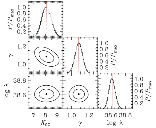
Figure 9: Probability distribution functions ($P$/$P_{\_}{\rm max}$) and confidence contours for parameter pairs (showing 68% and 95% confidence contours drawn) for our best-fit GC LMXB XLF model, which is based on 595 sources in 24 galaxies (see Section 4.4 for details). The vertical red dotted lines and solid black points indicate the median values of each parameter.

In Figure 8, the dotted purple curve shows our best-fit solution and residuals, and Figure 9 provides probability distribution functions and co-variance contour planes for the parameters $K_{\_}{\rm GC}$, $\gamma$, and $\lambda$. The best-fit model provides a good characterization of the broader shape and normalization of the GC LMXB XLF for our sample. We find a relatively shallow power-law slope $\gamma\approx 1.1$ with a cut-off at $\lambda\approx 4\times 10^{38}$ erg s^-1, just above the Eddington limit of an $\approx$2–3 $M_{\_}\odot$ neutron star, a feature that has long been noted in LMXB XLFs (see, e.g., the review by Fabbiano 2006).

Table 8: Best Fit Parameters for Global Fits

				$M_{\_}\star$-and-$S_{\_}N$-Dependent
Parameter		$M_{\_}\star$-Dependent					Z12
Name	Units	Field	GC LMXBs	Field (No Priors)	Field (Priors)	All LMXBs	Value
(1)	(2)	(3)	(4)	(5)	(6)	(7)	(8)
LMXB Population		Field	GC	Field	Field	Field + GC	Field + GC
$N_{\_}{\rm det}$		1285†	595	1285†	1285†	1880†
Field LMXB Component
$K_{\_}{M}$ or $K_{\_}{\rm in\mbox{-}situ}$	($10^{11}$ $M_{\odot}$)-1	60.9${}^{+6.7}_{\_}{-6.9}$	…	42.4${}^{+9.1}_{\_}{-7.9}$	42.7${}^{+6.5}_{\_}{-6.0}$	34.9${}^{+9.5}_{\_}{-6.9}$	$41.5\pm 11.5$
$\alpha_{\_}1$		1.00${}^{+0.06}_{\_}{-0.06}$	…	0.98${}^{+0.09}_{\_}{-0.11}$	1.02${}^{+0.07}_{\_}{-0.08}$	1.07${}^{+0.10}_{\_}{-0.12}$	1.02${}^{+0.07}_{\_}{-0.08}$
$L_{\_}b$	$10^{38}$ erg s-1	0.49${}^{+0.07}_{\_}{-0.04}$	…	0.45${}^{+0.07}_{\_}{-0.05}$	0.45${}^{+0.06}_{\_}{-0.04}$	0.52${}^{+0.17}_{\_}{-0.11}$	$0.546^{+0.043}_{\_}{-0.037}$
$\alpha_{\_}2$		2.12${}^{+0.07}_{\_}{-0.06}$	…	2.43${}^{+0.18}_{\_}{-0.15}$	2.50${}^{+0.18}_{\_}{-0.14}$	2.27${}^{+0.17}_{\_}{-0.13}$	2.06${}^{+0.06}_{\_}{-0.05}$
$L_{\_}{b,2}^{\ddagger}$	$10^{38}$ erg s-1	…	…	…	…	…	$5.99^{+0.95}_{\_}{-0.67}$
$\alpha_{\_}3^{\ddagger}$	…	…	…	…	…	…	$3.63^{+0.67}_{\_}{-0.49}$
$\log Lc$	$\log$ erg s-1	40.0∗	…	…	…	…	$40.04^{+0.18}_{\_}{-0.16}$
GC-Related LMXB Component
$K_{\_}{\rm GC}$ or $K_{\_}{\rm seed}$	($10^{11}M_{\_}\odot)^{-1}$ $S_{\_}N^{-1}$	…	8.08${}^{+0.42}_{\_}{-0.41}$	5.00${}^{+0.67}_{\_}{-0.61}$	5.10${}^{+0.53}_{\_}{-0.52}$	12.63${}^{+0.62}_{\_}{-0.59}$	…
$\gamma$		…	1.08${}^{+0.04}_{\_}{-0.04}$	1.21${}^{+0.11}_{\_}{-0.13}$	1.09${}^{+0.04}_{\_}{-0.04}$	1.12${}^{+0.07}_{\_}{-0.08}$	…
$\log\lambda$	$\log$ erg s-1	…	38.61${}^{+0.05}_{\_}{-0.04}$	38.66${}^{+0.10}_{\_}{-0.10}$	38.61${}^{+0.04}_{\_}{-0.04}$	38.50${}^{+0.05}_{\_}{-0.05}$	…
$C$		887	676	792	793	888	…
$C_{\_}{\rm exp}$		832	655	763	759	813	…
$C_{\_}{\rm var}$		1363	903	1273	1265	1403	…
$P_{\_}{\rm null}$		0.136	0.476	0.417	0.337	0.045	…
Calculated Parameters
$\log$($\alpha_{\_}{M}$ or $\alpha_{\_}{\rm in\mbox{-}situ}$)	$\log$ erg s-1 $M_{\_}\odot^{-1}$	29.17${}^{+0.03}_{\_}{-0.03}$	…	28.76${}^{+0.07}_{\_}{-0.07}$	28.75${}^{+0.06}_{\_}{-0.06}$	28.86${}^{+0.07}_{\_}{-0.08}$	$29.2\pm 0.1$
$\log$($\kappa_{\_}{\rm GC}$ or $\kappa_{\_}{\rm seed}$)	$\log$ erg s-1 $M_{\_}\odot^{-1}$ $S_{\_}N^{-1}$	…	28.55${}^{+0.03}_{\_}{-0.03}$	28.38${}^{+0.05}_{\_}{-0.06}$	28.38${}^{+0.05}_{\_}{-0.05}$	28.67${}^{+0.03}_{\_}{-0.04}$	…

Note.—Col.(1) and (2): Parameter and units. Col.(3)–(7): Value of each parameter for the various global models applied throughout this paper. Col.(8): Comparison values of LMXB scaling relations from Zhang et al. (2012).
^†Numbers include contributions from 47 background sources with $S<2\times 10^{-15}$ erg cm^-2 s^-1 (see Section 4.1).
^‡Parameter was used in Z12, but not in our study.

We find that our model provides a good overall characterization of the GC LMXB XLFs for the sample ($P_{\_}{\rm null}=0.476$; see Table 8). On a galaxy-by-galaxy basis, the model is a good fit ($P_{\_}{\rm null}\lower 2.15277pt\hbox{$\;\buildrel>\over{\sim}\;$}0.01$) to the GC XLFs for 20 out of the 21 galaxies with X-ray detected GCs (see Table 7). The three galaxies that did not have any GCs detected are consistent with predictions, as a result of these galaxies having either low stellar mass (NGC 4377 and NGC 7457) or shallow Chandra data (NGC 4406). The one galaxy, for which our GC-XLF model provides a poor characterization of the data, NGC 1399, is the most GC-rich galaxy in our sample.

The failing of the GC LMXB XLF model in NGC 1399 is thus likely due to unmodeled physical variations in the GC population. For example, red, metal-rich GC populations are observed to contain a larger fraction of bright LMXBs than blue, metal-poor GCs (e.g., Kundu et al. 2007; Kim et al. 2013; D’Abrusco et al. 2014; Mineo et al. 2014; Peacock & Zepf 2016; Peacock et al. 2017), and the fraction of metal-rich versus metal-poor GCs varies between galaxies (e.g., Brodie & Strader 2006). For the case of NGC 1399, detailed studies suggest that the red-to-blue ratio of GCs could be somewhat larger than most galaxies in our sample (e.g., Paolillo et al. 2011; D’Ago et al. 2014).

In a forthcoming paper, we will assess in more detail the properties of the LMXB populations in the GCs in our sample. Aside from the case of NGC 1399, the GC LMXB XLF model provides a good model to the GC LMXB data for the sample as a whole. We use parameters from our GC LMXB model in the next section to inform the shape of a GC-seeded LMXB contribution to the field LMXB XLF.

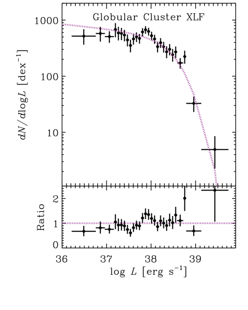
Figure 8: (Top) Best-fit completeness-corrected XLF for X-ray sources directly coincident with GCs (filled circles with 1$\sigma$ errors). This sample includes 595 such sources collected from the 24 elliptical galaxies in our sample. Our best-fitting power-law with exponential decay model is shown as a dotted purple curve. (Bottom) Ratio of data to model for our best-fit model. The dotted purple horizontal line at ratio = 1 has been indicated for reference.

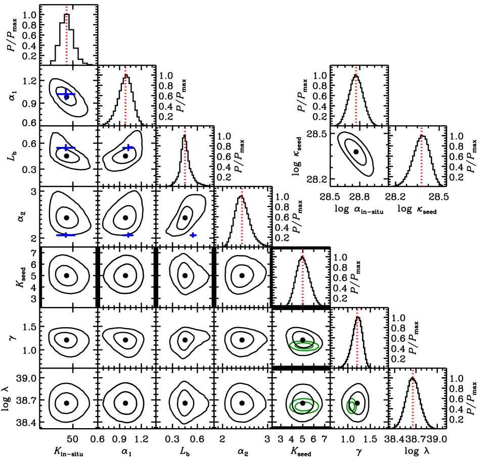
Figure 10: Probability distribution functions ($P$/$P_{\_}{\rm max}$) and confidence contours for parameter pairs (showing 68% and 95% confidence contours) for our best-fit field LMXB model, which is based on 1238 sources in 24 galaxies and uses flat priors on all parameters (see Section 4.5 for details). The parameters track the XLFs of LMXB populations that are presumed to form both in situ ($K_{\_}{\rm in\mbox{-}situ}$, $\alpha_{\_}1$, $L_{\_}b$, and $\alpha_{\_}2$) and those seeded from GCs ($K_{\_}{\rm seed}$, $\gamma$, and $\lambda$). The distribution functions for the integrated $L_{\_}{\rm X}$(in-situ)/$M_{\_}\star$ ($\alpha_{\_}{\rm in\mbox{-}situ}$) and $L_{\_}{\rm X}$(seed)/$M_{\_}\star$/$S_{\_}N$ ($\kappa_{\_}{\rm seed}$), implied by our model, are shown in the upper-right panels. Comparison values and 1$\sigma$ errors from Zhang et al. (2012) for all LMXB populations within elliptical galaxies are indicated with blue crosses in the in-situ parameterization. We also show resulting contours on $K_{\_}{\rm seed}$, $\gamma$, and $\lambda$ for the case where direct-GC LMXB best-fit model priors are used on $\gamma$ and $\lambda$ (green contours); these priors are informative, and the resulting values are consistent with the case where flat priors are used.

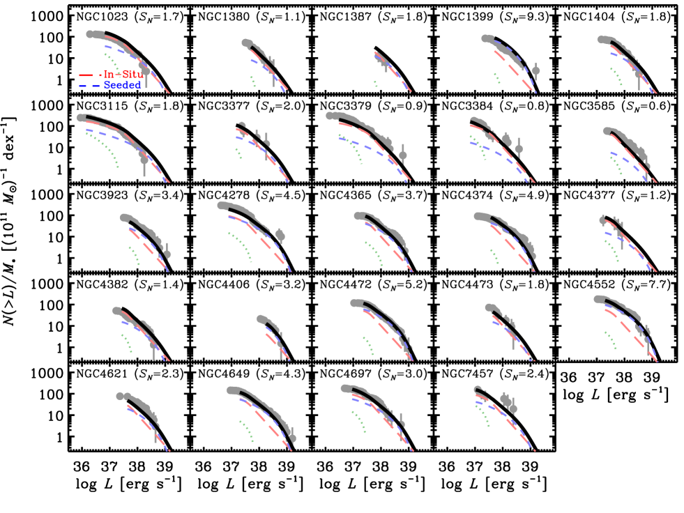
Figure 11: Same as Figure 5, but with the global model plotted. This model includes contributions from the CXB (green dotted curves), in-situ field LMXBs presumed to form within the galactic field (red long-dashed curves), and GC-seeded field LMXBs (short-dashed blue curves) that are expected to have originated in GCs. The model uses flat priors on all parameters in the fit (see Section 4.5 for details).

4.5 In-Situ and GC-Seeded Field LMXB XLF Model

We chose to revisit our fitting of the field LMXB XLF data using a two-component model consisting of an LMXB population that forms in situ and has an XLF that scales with stellar mass, plus a GC-seeded LMXB population with XLF normalization that scales with stellar mass and global $S_{\_}N$. The observed field LMXB XLF for a given galaxy is thus modeled following:

$$\frac{dN_{\_}{\rm field}}{dL}=\xi(L)\left[\frac{dN_{\_}{\rm in\mbox{-}situ}}{dL}+\frac{dN_{\_}{\rm seeded}}{dL}+{\rm CXB}\right],$$ (9)

where $dN/dL$(in-situ) and $dN/dL$(seeded) follow the functional forms provided in Eqns. (6) and (8), respectively, with $S_{\_}N$ being used here instead of $S_{\_}{N,{\rm loc}}$ in Eqn. (8).

In total, we fit for 7 parameters, including four parameters related to the in-situ component ($K_{\_}{\rm in\mbox{-}situ}$, $\alpha_{\_}1$, $L_{\_}b$, and $\alpha_{\_}2$; via Eqn. (6)) and three for the GC-seeded component ($K_{\_}{\rm seeded}$, $\gamma$, and $\lambda$; via Eqn. (8)). Following the fitting procedures discussed above (i.e., calculating the $C$ statistic via eqn (7) and using an MCMC technique to determine uncertainties) we determined the best-fit solution and parameter uncertainties for our model. We chose to fit the data for two scenarios: one in which all parameters varied freely without informative priors (i.e., flat priors), as well as a scenario in which informative priors were implemented on $\gamma$ and $\lambda$, based on the GC LMXB fit PDFs determined in Section 4.4.

In Table 8 (Col. (5) and (6)), we list the best-fit parameter values, uncertainties, and statistics for our model, including the cases with and without informative priors on $\gamma$ and $\lambda$. We graphically show the parameter PDFs and their correlations in Figure 10 (for the case with informative priors). From this representation, it is clear that all seven parameters are well constrained by our data, and we find this to be the case whether or not informative priors are implemented. The model provides an improvement in fit quality over the stellar-mass dependent model presented in Section 4.3 ($P_{\_}{\rm null}=0.337$ and 0.417 with and without informative priors, respectively). Furthermore, we find that $K_{\_}{\rm GC}$ is greater than zero at the $>$99.999% confidence level whether or not informative priors are implemented, providing further strong evidence that this component is required.

The above analysis confirms that the field LMXB population has a non-negligible contribution from sources that are correlated with the GC $S_{\_}N$, strongly indicating that GCs seed the field LMXB population. Further support for this scenario is seen in the good agreement between the shape of the GC-seeded and GC LMXB XLFs. Specifically, when informative priors are not implemented, the best-fit values for $\gamma$ and $\lambda$ are well constrained for the seeded population, and the values of these parameters are in good agreement with those from the direct GC population (Col. (3) of Table 8), consistent with a connection between the populations. However, we find that our GC LMXB priors on $\gamma$ and $\lambda$ are informative on the GC-seeded field LMXB population, and when implemented, result in tighter constraints on all parameters.

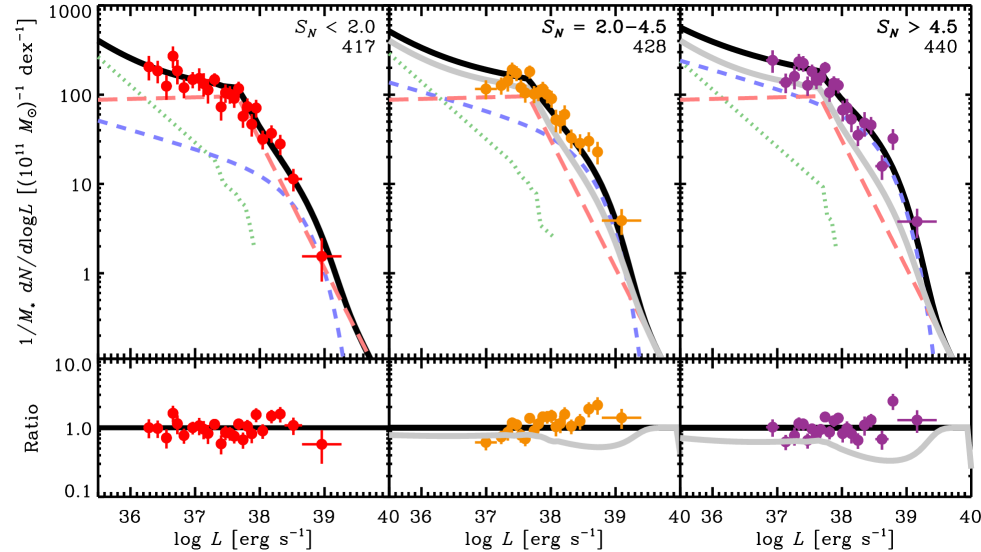
Figure 12: Completeness-corrected and stellar-mass-normalized field LMXB XLFs for subsamples of galaxies in bins of global $S_{\_}N$. All 1238 field LMXBs and 47 background sources with $S<2\times 10^{-15}$ erg cm^-2 s^-1 are represented here. For each panel, the $S_{\_}N$ range and number of X-ray detected sources are indicated in the upper right-hand corners. Our best-fit XLF model (based on flat priors of all parameters) is shown as a solid black curve, and contributions from in-situ LMXBs (red long-dashed curves), GC-seeded LMXBs (blue short-dashed curves), and CXB sources (green dotted curves) are indicated. Residuals (ratio of data-to-model) are provided in the bottom panels. For ease of comparison between panels, we repeated the $S_{\_}N<2$ best-fit curve (gray curve) in subsequent panels corresponding to higher $S_{\_}N$ values. As $S_{\_}N$ increases, the influence of GC seeding becomes more prominent, leading to more field LMXBs per unit stellar mass and a shallower-sloped XLF at $L\lower 2.15277pt\hbox{$\;\buildrel>\over{\sim}\;$}3~{}\times 10^{37}$ erg s^-1.

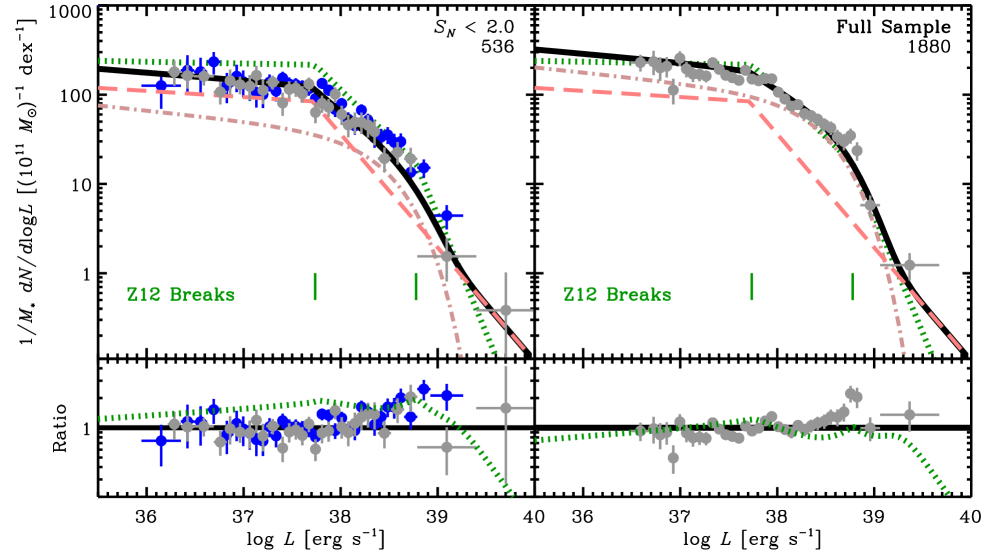
Figure 13: Completeness-corrected and stellar-mass-normalized total LMXB XLFs for galaxies with $S_{\_}N<2$ (left) and all sources (right), with residuals (bottom panels). In each panel, we provide our best-fit overall model (black), and the in-situ field (long-dashed faded red) and GC-related (combined field and direct GC; dot-dashed faded brown) model contributions. In the left panel, we also show the LMXB XLF from L19 (blue data points), which is measured from low SFR/$M_{\_}\star$ regions in primarily late-type galaxies that have $S_{\_}N<2$. We also show the best-fit model from Zhang et al. (2012) as dotted green curves and indicate the locations of their two power-law break luminosities.

To better assess the quality of our model, we evaluated the fit quality it provides to the field LMXB XLF of each galaxy. In Figure 11, we display the stellar-mass normalized observed XLF along with the best-fit $M_{\_}\star$-and-$S_{\_}N$-dependent model (based on flat priors) and its in-situ and GC-seeded model components shown separately. In Table 7, we list the statistical fit quality for each galaxy for the case of flat priors. In all cases, the individual field LMXB XLF is well described by this model, with $P_{\_}{\rm Null}\geq 0.069$ for all galaxies (see Col.(8) and (9) in Table 7).

With the exception of galaxies with $S_{\_}N\lower 2.15277pt\hbox{$\;\buildrel<\over{\sim}\;$}2$, our model suggests that the field LMXB XLFs of our galaxy sample has significant, and often dominant, contributions from seeded GCs at $L\lower 2.15277pt\hbox{$\;\buildrel>\over{\sim}\;$}10^{38}$ erg s^-1. At lower luminosities, $L\lower 2.15277pt\hbox{$\;\buildrel<\over{\sim}\;$}10^{38}$ erg s^-1, the in situ LMXB population is generally dominant for most galaxies with $S_{\_}N\lower 2.15277pt\hbox{$\;\buildrel<\over{\sim}\;$}4$.

Figure 12 shows the completeness corrected, stellar-mass-normalized field LMXB XLFs (in $dN/d\log L$ differential form) for combined subsamples of galaxies divided into bins of $S_{\_}N$. This view demonstrates that as $S_{\_}N$ increases, the field LMXB XLF increases in normalization and transitions from a broken power-law with a single obvious break to a shallower slope between $L\approx$ (3–100) $\times 10^{37}$ erg s^-1. For the highest $S_{\_}N$ bin ($S_{\_}N>4.5$), the field LMXB XLF appears to take on a three-sloped power-law, with breaks near $5\times 10^{37}$ erg s^-1 and $5\times 10^{38}$ erg s^-1. The apparent break locations are consistent with those that have been reported in the literature (see, e.g., Gilfanov 2004; Zhang et al. 2012), based on global fits to LMXB XLFs that include both field and GC sources combined. For example, the Zhang et al. (2012) break locations are at $L\approx 3\times 10^{37}$ erg s^-1 and $5\times 10^{38}$ erg s^-1. From our analysis, the low and high $L$ breaks can be attributed to the in-situ and GC-seeded populations, respectively; however, it is unclear from our data whether the GC seeded LMXB population also has a low-$L$ break ($L\approx 3\times 10^{37}$ erg s^-1), although some studies suggest this may be the case (e.g., Voss et al. 2009). We discuss the physical origins of this break in the Discussion section (Section 5) below.

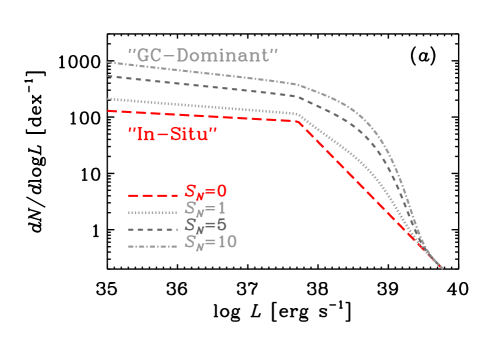
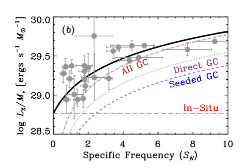
Figure 14: ($a$) LMXB XLF models (based on Col. (4) and (5) from Table 8) for various values of GC $S_{\_}N$ (see annotations). The XLF models are all appropriate for a galaxy mass of $M_{\_}\star=10^{11}$ $M_{\odot}$. The model transitions from a single-break broken power-law at $S_{\_}N=0$ to a more complex shape and higher normalization at larger $S_{\_}N$ due to the added contribution from GC LMXBs. ($b$) Integrated LMXB $L_{\_}{\rm X}/M_{\_}\star$ versus $S_{\_}N$ for our LMXB model (black solid curve), with contributions from in situ (red long-dashed), GC-seeded field (blue short-dashed), and direct GC (purple dotted) LMXBs shown. The overall LMXB population originating in GCs is shown as a brown dot-dashed curve. Values of $L_{\_}{\rm X}/M_{\_}\star$, and 1$\sigma$ uncertainties, for each of the 24 galaxies in our sample are shown as gray points with error bars. These values were determined by integrating best-fit broken power-law models to the total XLFs of each galaxy, as per the techniques described in Section 4.2.

4.6 Putting it All Together: A Global LMXB XLF Model for Elliptical Galaxies

The above analyses of the field and GC LMXB XLFs indicate that we can successfully model the LMXB XLF of a given galaxy as consisting of both in-situ and GC seeded field LMXBs, as well as direct-counterpart GC LMXBs, with the seeded and direct-counterpart GC LMXB XLFs having similar shapes. When combining the field and GC LMXB data sets and model statistics (i.e., combining Col. (5) and (4) in Table 8), we find $P_{\_}{\rm null}=0.280$, suggesting a very good overall characterization of both field and direct-counterpart GC LMXB populations. Given the success of this framework, as well as the fact that our galaxy sample does not have substantial diversity in stellar-mass-weighted age (see Section 3.1), we do not attempt to model how the in situ field LMXB population evolves with age. However, in Section 5, we contextualize the constraints placed on the field LMXB populations studied here and in previous investigations, as well as the constraints on the age-dependence of LMXB populations (e.g., Fragos et al. 2013a, 2013b; Lehmer et al. 2016; Aird et al. 2017).

Given the similarities between the seeded and direct-counterpart GC LMXB XLF solutions, we attempted to fit the entire data set (i.e., both field and GC LMXB populations taken together) using a single model for the GC population. Using the priors on the direct-counterpart GC LMXB and field LMXB models determined in Sections 4.4 and 4.5, respectively (i.e., the models summarized in Table 8, Col.(4) and (5), respectively), we fit the total LMXB XLFs (including both direct-counterpart GC LMXBs and field LMXBs) to test whether our cumulative model fits are acceptable for all galaxies and cumulatively for the whole sample. In practice, we made use of Equation (8) when modeling GC LMXBs XLF components, using normalizations that consist of $K_{\_}{\rm GC}$ and $K_{\_}{\rm seeded}$, which scale with $S_{\_}{N,{\rm loc}}$ and $S_{\_}N$, respectively. To track the relative scalings in our MCMC procedure fit to all sources, we drew from previous MCMC chains originating from our fits to direct-counterpart and seeded GC LMXB populations to implement priors on each of the respective normalizations, and we quote a single normalization that includes the sum of the priors (i.e., $K_{\_}{\rm seed}+K_{\_}{\rm GC}$). We implemented flat priors for all other parameters in the fits.

The resulting fit parameters are listed in Col.(7) of Table 8. The fit quality is acceptable ($P_{\_}{\rm null}\approx 0.045$), albeit less favorable than the case where we utilize separate direct-counterpart and seeded GC XLF solutions (i.e., the combined models from Col.(4) and (5) of Table 8).

In Figure 13, we show the completeness-corrected and CXB subtracted XLFs for a subsample of galaxies with $S_{\_}N<2$ and the full galaxy sample. The $S_{\_}N<2$ subsample is shown for comparison with late-type galaxy samples, which primarily fall into this $S_{\_}N$ regime (see H13). We show the L19 LMXB XLF data (blue points), which were constrained from subgalactic regions with SFR/$M_{\_}\star$ $\lower 2.15277pt\hbox{$\;\buildrel<\over{\sim}\;$}10^{-10}$ yr^-1. We find a factor of $\approx$1.5–2 elevated residuals above $10^{38}$ erg s^-1 for the late-type galaxy LMXBs. Excesses of LMXBs in this luminosity regime were also noted by L19 in regions of late-type galaxies with relatively active SF activity ($-10.5<\log$ SFR/$M_{\_}\star<-10$) compared to lower SF activity ($\log$ SFR/$M_{\_}\star<-10.5$). This could potentially implicate an age effect, in which younger LMXB populations have an excess of $10^{38}$ erg s^-1 sources. Quantifying this effect is beyond the scope of the current paper.

In both panels of Figure 13, we compare our best-fit $M_{\_}\star$-and-$S_{\_}N$-dependent XLF model (black curves) with the stellar-mass-dependent model from Zhang et al. (2012; Z12; green dotted curves), which is based on a three-sloped broken power-law model with two break locations (indicated in Figure 13). Consistent with what we found for the field LMXB XLF, our model reproduces the two-break nature of the LMXB XLF, with the break locations consistent with those seen by Z12. We find that the Z12 model itself overpredicts the observed total LMXB XLFs for $S_{\_}N<2$ galaxies by a factor of $\approx$2 for the $L\lower 2.15277pt\hbox{$\;\buildrel<\over{\sim}\;$}10^{39}$ erg s^-1 population. Comparison between the Z12 model and our full-sample LMXB XLF shows very good agreement. This can be reconciled by the fact that the Z12 sample has substantial overlap with our own sample, which is dominated by galaxies with high-$S_{\_}N$ and GC LMXBs. Thus, a single $M_{\_}\star$-dependent model (i.e., the Z12 model) would not be applicable for low-$S_{\_}N$ galaxies, which are dominated by field LMXBs at $L\lower 2.15277pt\hbox{$\;\buildrel<\over{\sim}\;$}10^{38}$ erg s^-1. Given that the late-type galaxy LMXB XLF is in good agreement with the $S_{\_}N<2$ LMXB XLF at $L\lower 2.15277pt\hbox{$\;\buildrel<\over{\sim}\;$}10^{38}$ erg s^-1, this result further implies that $M_{\_}\star$-dependent LMXB XLFs derived for massive elliptical galaxies overpredict the numbers of LMXBs in this luminosity range for late-type galaxies. However, at $L\lower 2.15277pt\hbox{$\;\buildrel>\over{\sim}\;$}3\times 10^{38}$ erg s^-1, the late-type galaxy LMXBs may exceed such predictions (see bottom-left panel of Fig. 13).

5 Discussion

We find that, after excluding background X-ray sources and LMXBs coincident with GCs, the remaining field LMXB populations in elliptical galaxies show both signatures of LMXBs that originated in GCs (via GC seeding), as well as a non-negligible population of LMXBs that formed in situ through secular binary evolution. We construct a framework describing how the LMXB XLF in elliptical galaxies varies with GC $S_{\_}N$, that provides a statistically acceptable model to all 24 elliptical galaxies in our sample.

Figure 14 illustrates our final model of LMXB populations in elliptical galaxies, which is derived from the model parameters in Col.(4) and (5) from Table 8. In Figure 14$a$, we show the stellar-mass-normalized LMXB XLF model at various $S_{\_}N$ values, illustrating the variation of the LMXB XLF going from a broken power-law XLF for an in-situ-dominated population at $S_{\_}N\lower 2.15277pt\hbox{$\;\buildrel<\over{\sim}\;$}2$ to a more numerous population of GC-related LMXBs with a more complex XLF shape at higher $S_{\_}N$.

Figure 14$b$ tracks the stellar-mass-normalized integrated luminosity, $L_{\_}{\rm X}/M_{\_}\star$, of LMXB populations as a function of $S_{\_}N$. For our model, the expectation value of $L_{\_}{\rm X}/M_{\_}\star$ can be calculated following:

$$L_{\_}{\rm X}/M_{\_}\star=\int_{\_}{L_{\_}{\rm lo}}^{L_{\_}c}\left(\frac{dN_{\_}{\rm in\mbox{-}situ}}{dL}+\frac{dN_{\_}{\rm seed}}{dL}+\frac{dN_{\_}{\rm GC}}{dL}\right)\frac{L}{M_{\_}\star}\;dL.\\$$ (10)

Integrating from $L_{\_}{\rm lo}=10^{36}$ erg s^-1 to the cut-off luminosity at $L_{\_}c=10^{40}$ erg s^-1 gives:

$$L_{\_}{\rm X}/M_{\_}\star=\alpha_{\_}{\rm in\mbox{-}situ}+\kappa_{\_}{\rm GC+seed}S_{\_}N,$$

$$\log(\alpha_{\_}{\rm in\mbox{-}situ}/[{{\rm erg~{}s^{-1}~{}M_{\_}\odot^{-1}}}])=28.76\pm 0.07,$$

$$\log(\kappa_{\_}{\rm GC+seed}/[{{\rm erg~{}s^{-1}~{}M_{\_}\odot^{-1}}}])=28.77^{+0.06}_{\_}{-0.07}.$$ (11)

Here, we define $\alpha_{\_}{\rm in\mbox{-}situ}\equiv L_{\_}{\rm X,in~{}situ}/M_{\_}\star$ and $\kappa_{\_}{\rm GC+seed}\equiv(L_{\_}{\rm X,GC}+L_{\_}{\rm X,seed})/M_{\_}\star/S_{\_}N$, as integrated luminosity scaling relations for in-situ and combined direct-GC plus GC-seeded populations, respectively. In Figure 14$b$, we show our best-fit model $L_{\_}{\rm X}/M_{\_}\star$ versus $S_{\_}N$ as a solid black line, and highlight the contributions from in-situ, GC-seeded, and GC populations separately. For comparison, we have overlaid the estimated $L_{\_}{\rm X}/M_{\_}\star$ values for each of the 24 galaxies, based on integrating best-fitting broken power-law models, appropriate for the full LMXB population of each galaxy (following the methods described in Section 4.3).

In terms of integrated luminosity, we find that galaxies above (below) $S_{\_}N\approx 1.5$ are dominated by GC-produced (in-situ) LMXBs. As discussed in Section 4.6 above, typical late-type galaxies are observed to have $S_{\_}N\approx 1$, with the majority having $S_{\_}N<2$, suggesting that although GC-produced LMXBs dominate the elliptical galaxies in our sample, they are not expected to dominate the integrated LMXB luminosities of more typical late-type galaxies in the nearby universe. Furthermore, as presented in $\S$4.6, there is evidence that the late-type galaxy LMXB XLF contains an excess of luminous LMXBs ($L\lower 2.15277pt\hbox{$\;\buildrel>\over{\sim}\;$}10^{38}$ erg s^-1) compared with the $S_{\_}N<2$ elliptical galaxy LMXB population (see Fig. 13$a$), potentially due to an underlying age-dependence in the LMXB population.

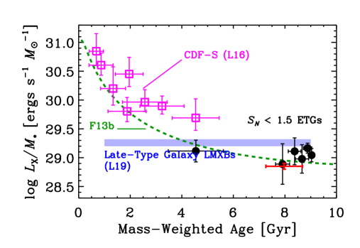
Figure 15: Integrated field LMXB XRB luminosity per unit stellar mass, $L_{\_}{\rm X}/M_{\_}\star$, versus stellar-mass weighted age for elliptical galaxies with $S_{\_}N<1.5$ (black circles with 1$\sigma$ uncertainties). These galaxies are expected to have field LMXB populations dominated by the in-situ formation channel, for which we expect $L_{\_}{\rm X}/M_{\_}\star$ to be stellar-age dependent. The red error bars indicate 1$\sigma$ standard deviations on the mass-weighted stellar ages and the uncertainty on the in-situ $L_{\_}{\rm X}/M_{\_}\star$ value derived for the full sample. The blue band shows the mean $L_{\_}{\rm X}/M_{\_}\star$ value for LMXBs derived for late-type galaxies from Lehmer et al. (2019), and the magenta open squares (with 1$\sigma$ uncertainties) show estimates from the Lehmer et al. (2016) stacking analyses from the 6 Ms CDF-S (see text for details). The green dashed curve shows the predicted XRB population synthesis model trend from Fragos et al. (2013b), based on the evolving mass-weighted stellar age of the Universe. The collection of constraints thus far are basically consistent with the trends predicted by the Fragos et al. (2013b) population synthesis framework, however, significant uncertainties remain.

In addition to the differences between late-type and elliptical galaxy LMXB XLFs, there is evidence that the average integrated LMXB luminosity scaling with stellar mass ($L_{\_}{\rm X}/M_{\_}\star$) increases with redshift between $z\approx$ 0–2 (Lehmer et al. 2007, 2016; Aird et al. 2017), signifying younger LMXB populations (at high redshift) contain more luminous in-situ LMXBs. Using the mass-weighted stellar ages for our galaxies, based on the SFHs presented in Section 3.1, we searched for any residual trends between the field-LMXB $L_{\_}{\rm X}/M_{\_}\star$ and age. To avoid contamination from GC LMXBs, we limited our sample to elliptical galaxies with $S_{\_}N<1.5$, which includes seven of the 24 galaxies in our sample (NGC 1380, 3379, 3384, 3585, 4377, 4382, and 4697). These galaxies span a mass-weighted stellar age range of $\approx$4–9 Gyr and have comparable values of field-LMXB $L_{\_}{\rm X}/M_{\_}\star$ ($\log L_{\_}{\rm X}/M_{\_}\star\approx 29$), which we show in Figure 15.

In Figure 15, we have overlaid estimated values of $L_{\_}{\rm X}$(LMXB)/$M_{\_}\star$ versus mass-weighted stellar age for stacked constraints from Lehmer et al. (2016; L16), which are based on results from a 6 Ms exposure of the Chandra Deep Field-South (CDF-S; Luo et al. 2017). These are mean values of $L_{\_}{\rm X}$(LMXB)/$M_{\_}\star$ at different redshifts, in which the redshift has been converted into a mass-weighted stellar age for the population. These mass-weighted stellar ages were calculated by first extracting synthesized galaxy catalogs from the Millenium II cosmological simulation from Guo et al. (2011) that had the same SFR and $M_{\_}\star$ selection ranges as those adopted by Lehmer et al. (2016). These galaxy catalogs contain estimates of the mass-weighted stellar ages for each galaxy. The mass-weighted stellar age of the entire galaxy population (catalog) is then estimated, and a standard deviation of the population is calculated to estimate the uncertainty. Given this highly model-dependent procedure, we provide these points only for guidance and note that their true uncertainties are likely to be much larger than those shown.

The L16 CDF-S constraints indicate that galaxies with mass-weighted stellar ages in the range of $\approx$0.5–5 Gyr, have $\log(L_{\_}{\rm X}$[LMXB]/$M_{\_}\star)=$ 29.5–31, generally well above the $L_{\_}{\rm X}/M_{\_}\star$ values for the elliptical galaxies in our sample (including those with the highest $S_{\_}N$). Since we do not expect that LMXBs that originate in GCs would have XLFs or $L_{\_}{\rm X}$[GC-LMXB]/$M_{\_}\star$ values that depend on stellar age, it is likely that these high redshift LMXB populations would be dominated by in-situ LMXBs. In Figure 15, we show $L_{\_}{\rm X}/M_{\_}\star$ versus mass-weighted stellar age from the XRB population synthesis model of Fragos et al. (2013b; F13b, green dashed curve), which is based entirely on the in situ formation channel. Qualitatively, the constraints for $S_{\_}N<1.5$ elliptical galaxies studied here, the late-type galaxies presented in Lehmer et al. (2019), and the CDF-S stacked data follow the F13b trend, providing support for a rapidly evolving in situ LMXB population that dominates for most galaxies, except for the most GC-rich elliptical galaxies.

Unfortunately, we are unable to find quantitative evidence for stellar-age dependence in the in situ formation rates of the elliptical galaxies studied here, due to a lack of diverse stellar ages in our sample. In future work, we can mitigate this limitation by using SFH information, similar to that presented in Section 2.3, combined with Chandra constraints on XRB populations for a combined late-type and elliptical galaxy sample. The XRB XLFs for members of this combined galaxy sample would contain non-negligible contributions from XRBs associated with stellar populations of all ages. In Lehmer et al. (2017), we presented preliminary work for the single case of the XRB population within M51, and were able to show that a stellar-age parameterized XLF model suggested that the XRB population integrated $L_{\_}{\rm X}/M_{\_}\star$ declines by 2.5–3 orders of magnitude from 10 Myr to 10 Gyr, similar to that shown in Figure 15. With the combined late-type and elliptical galaxy sample, we can constrain the evolution of the XRB XLF as a function of age without an explicit parameterization with age.

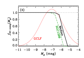
Figure A1: ($a$) Fraction of bright GCs ($M_{\_}g<-7$) as a function of galactocentric semi-major axis, $r/a$, for all 24 galaxies in our sample. Each annulus is elliptical in shape with position angle and axis ratio matching that of the $K_{\_}s$-band ellipse defined in Table 1. This distribution is used to weight GC completeness functions, which vary across the galaxies due to background variations. ($b$) Weighted GC completeness functions for the example case of NGC 1399 (green dashed curve) and the median of our sample (black solid curve). For comparison, the shape of the GC optical luminosity function from Kundu & Whitmore (2001) has been overlaid (red dotted curve). ($c$) Fraction of GCs with Chandra-detected point sources as a function of absolute magnitude. The fraction of X-ray detected sources drops rapidly with decreasing GC optical luminosity suggesting that most of the GCs below the HST detection thresholds will not host LMXBs.

Appendix A Globular Cluster Completeness and Local Specific Frequency

Quantifying the relative contributions of LMXBs associated with direct-GC counterparts and those seeded in the field requires that we obtain estimates of the local specific frequency, $S_{\_}{N,{\rm loc}}$, as well as the completeness of our HST data to detecting GCs that host LMXBs. We define the GC-LMXB completeness, $f_{\_}{\rm GC-LMXB}^{\rm recover}$ as the fraction of X-ray-detected sources for which we could identify a direct GC counterpart, if one were present. For a given galaxy, $f_{\_}{\rm GC-LMXB}^{\rm recover}$ will depend on HST exposure depths, the variation of the background light throughout the galaxy (primarily due to the galaxy light profile), the distribution of GCs throughout the galaxy, the intrinsic optical luminosity function of the GC population, and finally, the intrinsic fraction of X-ray sources that are associated with GCs as a function of optical luminosity.

We measured each of the above completeness factors using a series of techniques. We began by using simulations to measure the magnitude and background dependent completeness function for GCs in the galaxy NGC 1399, which contains the largest range of background levels for our galaxy sample and a rich GC population. Due to computation time limitations, our strategy was to determine a magnitude and background dependent parameterization for the completeness function for NGC 1399, and then apply that parameterization to other galaxies in our sample to assess completeness variations.

First, working with HST images for NGC 1399 in units of counts, we added 120,000 fake GCs, with absolute magnitudes in the range of $-10\leq M_{\_}g\leq-5$. The surface brightness distributions of our sources followed empirical King light profiles with parameters chosen to mimic the light profiles of detected GCs. The sources were implanted at random positions across the extent of the galaxies, covering all background levels. Following the procedures outlined in Section 3.2, we searched the fake images for source detections and calculated the GC recovery fraction as a function of background counts and apparent magnitude.

From these simulated recovery fractions, we generated an absolute-magnitude and background-count dependent parameterization that followed the observed behavior. To test whether our parameterization was robust, we repeated the above simulation process for NGC 1404 to generate recovery fraction diagrams in bins of background counts. We found that our NGC 1399-based parameterization, given simply local background counts in NGC 1404, correctly reproduced the simulated completeness functions very well with only a $\approx$0.5 mag deviation appearing at the highest background levels. To account for this deviation at high background levels, we based our final recovery fraction parametrization on the simulations for both NGC 1399 and NGC 1404, and we take this 0.5 mag deviation to be a conservative limit on the robustness of our parameterization.

For the remaining galaxies, we calculated completeness levels using the measured background levels within each of the galaxies and our parameterization for completeness as a function of background. the mean background levels in several concentric annuli from the galactic centers to the edges of the $K_{\_}s$-band ellipses. The annuli were elliptical in size and followed the axis ratios and position angles provided in Table 1. At each annulus, our completeness parameterization provides a magnitude-dependent completeness function. To assess the overall GC detection completeness for a given galaxy, we required knowledge of the spatial distribution of GCs throughout the galaxy, since the total population completeness will depend on the relative weightings on the local completeness functions. Using all GCs in our total elliptical galaxy sample with $M_{\_}g<-7$ mag (bright GCs that we are $\approx$100% complete to), we compiled the galaxy-sample-total distribution of GCs with respect to galactocentric offset (in units of fractional distance to the nearest edge of the galaxy), $w_{\_}{\rm GC}(r)\equiv N_{\_}{{\rm GC},r}/N_{\_}{\rm GC,tot}$, where $N_{\_}{{\rm GC},r}$ is the number of GCs within annuli of galactocentric semi-major axes $r/a$ and $N_{\_}{\rm GC,tot}$ is the total number of GCs within the whole sample. Figure A1($a$) shows $w_{\_}{\rm GC}(r)$ measured from the whole sample. Examination of the distributions of GCs within individual galaxies show consistency with this distribution, when such distributions can be measured reliably.

Using the galactocentric offset distribution of GCs, $w_{\_}{\rm GC}(r)$, as statistical weights, we derived a weighted completeness function for each galaxy following:

$$f_{\_}{\rm GC-comp}(M_{\_}g)=\sum_{\_}i^{n_{\_}{\rm r}}w_{\_}{\rm GC}(r_{\_}i)f_{\_}{\rm GC-comp}(M_{\_}g,r_{\_}i),$$ (A1)

where the summation takes place over $n_{\_}{\rm r}=10$ annuli. Here, $r_{\_}i$, $w_{\_}{\rm GC}(r_{\_}i)$, and $f_{\_}{\rm GC-comp}(M_{\_}g,r_{\_}i)$ are the radius (in units of the semimajor axis), fraction of GCs located in the annulus, and completeness function, respectively, appropriate for the $i$th annulus.

Figure A1(b) shows the weighted magnitude dependent completeness function for NGC 1399 and the median galaxy in our sample. In these cases, the HST data are complete to a 50% limiting F475W absolute magnitudes of $M_{\_}g\approx-6.2$ and $-5.8$ mag for NGC 1399 and the median, respectively. For context, in Figure A1(b), we overlay the shape of the best-fit Gaussian GC luminosity function from Kundu & Whitmore (2001),

$$\frac{dN_{\_}{\rm GC}}{dM_{\_}g}=A_{\_}{\rm GC}\exp\left[-\frac{(M_{\_}g-M_{\_}0)^{2}}{2\sigma^{2}}\right],$$ (A2)

where $A_{\_}{\rm GC}$ has been normalized arbitrarily, $M_{\_}0=-7.1$ mag (converted from $M_{\_}V=-7.4$ mag), and $\sigma=1.3$ mag. Based on these diagrams, it is clear that our HST data will not be fully complete to all GCs present within the galaxy.

We note, however, that the fraction of GCs that host X-ray detected sources is known to decline with decreasing GC luminosity. Using the known GC populations within all galaxies, we calculated the fraction of GCs coincident with X-ray detected objects as a function of GC absolute magnitude, $f_{\_}{\rm LMXBs}(M_{\_}g)$. In Figure A1($c$), we show our empirical version of $f_{\_}{\rm LMXBs}(M_{\_}g)$, which indeed shows a precipitous decline with decreasing GC optical luminosity.

Given the above ingredients, we can finally calculate the fraction of GCs that host LMXBs that would be identified as such using the following equation:

$$f_{\_}{\rm GC-LMXB}^{\rm rec}\approx\frac{\sum_{\_}{j=0}^{n_{\_}{\rm M}}(dN_{\_}{\rm GC}/dM_{\_}g)_{\_}jf_{\_}{\rm GC-comp}(M_{\_}g)_{\_}jf_{\_}{\rm LMXBs}(M_{\_}g)_{\_}j}{\sum_{\_}{j=0}^{n_{\_}{\rm M}}(dN_{\_}{\rm GC}/dM_{\_}g)_{\_}jf_{\_}{\rm LMXBs}(M_{\_}{g})_{\_}j},$$ (A3)

where the summations take place over $n_{\_}M=100$ bins of absolute magnitude from $-11\lower 2.15277pt\hbox{$\;\buildrel<\over{\sim}\;$}M_{\_}g\lower 2.15277pt\hbox{$\;\buildrel<\over{\sim}\;$}-3$ using linearly-interpolated values from our $f_{\_}{\rm GC-comp}$ and $f_{\_}{\rm LMXBs}$. Since the completeness functions vary somewhat from galaxy-to-galaxy, primarily due to distance variations, the value of $f_{\_}{\rm GC-LMXB}^{\rm rec}$ varies too. We find a full range of $f_{\_}{\rm GC-LMXB}^{\rm rec}=$ 89.0–99.6%, with a median completeness of 96.1%. This implies that our GC LMXB classifications are highly complete, and we are very unlikely to be misclassifying a substantial fraction of LMXBs coincident with GCs as field sources.

The GC completeness information obtained above allows us to estimate $S_{\_}{N,{\rm loc}}$ for our sample. For each galaxy, we first obtained an estimate of the total number of GCs that were present locally within the HST observational fields, $N_{\_}{\rm GC,loc}$, using Equation (A2) and our completeness functions (Equation A1). Specifically, we determined the value of $A_{\_}{\rm GC}$ from Equation (2) using the following equation:

$$A_{\_}{\rm GC}=\frac{N_{\_}{\rm GC,obs}}{\int\frac{dN_{\_}{\rm GC}}{dM_{\_}g}f_{\_}{\rm GC-comp}(M_{\_}g)dM_{\_}g}=\frac{N_{\_}{\rm GC,obs}}{\int f_{\_}{\rm GC-comp}(M_{\_}g)\exp\left[-\frac{(M_{\_}g-M_{\_}0)^{2}}{2\sigma^{2}}\right]dM_{\_}g},$$

where $N_{\_}{\rm GC,obs}$ is the number of GCs observed in the HST field of view. Given $A_{\_}{\rm GC}$, we estimated $N_{\_}{\rm GC,loc}$ as

$$N_{\_}{\rm GC,loc}=\int\frac{dN_{\_}{\rm GC}}{dM_{\_}g}dM_{\_}g.$$

Finally, values of $S_{\_}{N,{\rm loc}}$ were calculated following

$$S_{\_}{N,{\rm loc}}=N_{\_}{\rm GC,loc}10^{0.4(M_{\_}{V,{\rm loc}}+15)},$$ (A4)

where estimates of local absolute $V$-band magnitude, $M_{\_}{V,{\rm loc}}$, were obtained from our SED fitting procedure (see Section 3.1).

Appendix B X-ray Point Source Catalog

Table B1: X-ray point-source catalog and properties

Gal.		$\alpha_{\_}{\rm J2000}$	$\delta_{\_}{\rm J2000}$	$\theta$	$N_{\_}{\rm FB}$	$N_{\_}{\rm H}$		$\log F_{\_}{\rm FB}$	$\log L_{\_}{\rm FB}$	Loc.	Opt.
(NGC)	ID	(deg)	(deg)	(arcmin)	(counts)	($10^{22}$ cm-2)	$\Gamma$	(cgs)	(erg s-1)	Flag	Class
(1)	(2)	(3)	(4)	(5)	(6)–(7)	(8)–(9)	(10)–(11)	(12)	(13)	(14)	(15)
1023	1	02 40 04.07	+39 03 53.89	3.9	13.7$\pm$4.5	0.056	1.7	$-$15.2	37.0	3	U
	2	02 40 04.83	+39 04 25.65	3.8	24.5$\pm$5.7	0.056	1.7	$-$15.0	37.2	3	U
	3	02 40 04.94	+39 00 40.53	4.8	16.9$\pm$5.0	0.056	1.7	$-$14.9	37.3	3	U
	4	02 40 05.13	+39 05 06.94	3.9	110.1$\pm$12.6	0.823$\pm$0.539	1.90$\pm$0.64	$-$14.2	38.0	3	U
	5	02 40 05.81	+39 04 32.56	3.6	30.4$\pm$7.5	1.527$\pm$1.276	$<$2.57	$-$14.8	37.4	3	U
	6	02 40 07.52	+39 03 43.77	3.2	73.2$\pm$10.4	0.291$\pm$0.340	2.37$\pm$0.87	$-$14.6	37.6	3	U
	7	02 40 07.76	+39 03 14.00	3.2	118.1$\pm$12.8	$<$0.056	1.92$\pm$0.30	$-$14.3	37.9	3	U
	8	02 40 08.37	+39 01 59.18	3.5	76.2$\pm$10.6	0.504$\pm$0.493	2.25$\pm$0.94	$-$14.5	37.7	3	U
	9	02 40 08.64	+39 04 42.73	3.1	14.2$\pm$4.5	0.056	1.7	$-$15.2	37.0	3	U
	10	02 40 10.43	+39 04 09.94	2.7	15.5$\pm$4.4	0.056	1.7	$-$15.2	37.0	3	U
	11	02 40 10.45	+39 02 25.88	3.0	66.9$\pm$8.5	0.056	1.7	$-$14.6	37.6	3	U
	12	02 40 11.35	+39 05 29.79	3.0	48.5$\pm$8.8	$<$0.056	2.14$\pm$0.51	$-$14.8	37.4	3	U
	13	02 40 11.37	+39 06 09.86	3.4	25.6$\pm$5.7	0.056	1.7	$-$15.0	37.2	3	U
	14	02 40 12.56	+39 06 49.39	3.8	23.7$\pm$5.9	0.056	1.7	$-$15.0	37.2	3	U
	15	02 40 13.04	+39 00 51.77	3.6	3735.1$\pm$65.6	$<$0.056	$<$3.30	$-$12.9	39.3	3	U
	16	02 40 13.53	+39 01 33.09	3.0	181.2$\pm$15.5	$<$0.056	1.62$\pm$0.23	$-$14.1	38.1	3	U
	17	02 40 13.70	+39 04 04.12	2.0	93.6$\pm$11.6	7.333$\pm$1.447	$<$3.30	$-$14.1	38.1	1	F
	18	02 40 14.37	+39 02 50.95	2.1	8.9$\pm$3.5	0.056	1.7	$-$15.5	36.7	1	F
	19	02 40 15.56	+39 00 15.03	3.9	24.2$\pm$5.8	0.056	1.7	$-$14.9	37.3	3	U
	20	02 40 15.90	+39 07 23.95	3.9	23.3$\pm$6.0	0.056	1.7	$-$15.0	37.2	3	U

Note.—The full version of this table contains 4206 sources. An abbreviated version of the table is displayed here to illustrate its form and content. A description of the columns is provided in the text of Appendix B.

In Table B1, we provide the X-ray point source catalogs, based on the analyses presented in $\S\S$3.2 and 3.3. The columns include the following: Col.(1): Name of the host galaxy. Col.(2): point-source identification number within the galaxy. Col.(3) and (4): Right ascension and declination of the point source. Col.(5): Offset of the point source with respect to the average aim point of the Chandra observations. Col.(6) and (7): 0.5–7 keV net counts (i.e., background subtracted) and 1$\sigma$ errors. Col.(8)–(9) and (10)–(11): Best-fit column density $N_{\_}{\rm H}$ and photon index $\Gamma$, respectively, along with their respective 1$\sigma$ errors, based on spectral fits to an absorbed power-law model (TBABS${}_{\_}{\rm Gal}\times$ TBABS $\times$ POW in xspec). For sources with small numbers of counts ($<$20 net counts), we adopted only Galactic absorption appropriate for each galaxy and a photon index of $\Gamma=1.7$. Col.(12) and (13): the respective 0.5–8 keV flux and luminosity of the source. Col.(14): Flag indicating the location of the source within the galaxy. Flag=1 indicates the source is within the $K_{\_}s$-band footprint adopted in Table 1, and outside a central region of avoidance, if applicable. All XLF calculations are based on Flag=1 sources. Flag=2 indicates that the source is located in the central region of avoidance due to either the presence of an AGN or very high levels of source confusion. Flag=3 indicates that the source is outside the 20 mag arcsec^-2 $K_{\_}s$-band ellipse of the galaxy. Col.(15): HST classification of the source, whenever the source is within the footprint of the galaxy, as defined in Table 1. Classifications include field LMXBs (“F”), direct-GC LMXBs (“G”), background sources (“B”), and unclassified sources (“U”).

References

- Aird et al. (2017) Aird, J., Coil, A. L., & Georgakakis, A. 2017, MNRAS, 465, 3390
- Albareti et al. (2017) Albareti, F. D., Allende Prieto, C., Almeida, A., et al. 2017, ApJS, 233, 25
- Arnaud (1996) Arnaud, K. A. 1996, Astronomical Data Analysis Software and Systems V, 101, 17
- Basu-Zych et al. (2013) Basu-Zych, A. R., Lehmer, B. D., Hornschemeier, A. E., et al. 2013, ApJ, 774, 152
- Basu-Zych et al. (2016) Basu-Zych, A. R., Lehmer, B., Fragos, T., et al. 2016, ApJ, 818, 140
- Bertin & Arnouts (1996) Bertin, E., & Arnouts, S. 1996, A&AS, 117, 393
- Brodie, & Strader (2006) Brodie, J. P., & Strader, J. 2006, ARA&A, 44, 193
- Broos et al. (2010) Broos, P. S., Townsley, L. K., Feigelson, E. D., et al. 2010, ApJ, 714, 1582
- Broos et al. (2011) Broos, P. S., Townsley, L. K., Feigelson, E. D., et al. 2011, ApJS, 194, 2
- Broos et al. (2012) Broos, P., Townsley, L., Getman, K., et al. 2012, AE: ACIS Extract, ascl:1203.001
- Brorby et al. (2016) Brorby, M., Kaaret, P., Prestwich, A., et al. 2016, MNRAS, 457, 4081
- Cash (1979) Cash, W. 1979, ApJ, 228, 939
- Civano et al. (2016) Civano, F., Marchesi, S., Comastri, A., et al. 2016, ApJ, 819, 62
- Cheng et al. (2018) Cheng, Z., Li, Z., Xu, X., et al. 2018, ApJ, 858, 33
- Civano et al. (2016) Civano, F., Marchesi, S., Comastri, A., et al. 2016, ApJ, 819, 62
- Clark, & Parkinson (1975) Clark, D. H., & Parkinson, J. H. 1975, Nature, 258, 408
- D’Abrusco et al. (2014) D’Abrusco, R., Fabbiano, G., Mineo, S., et al. 2014, ApJ, 783, 18
- D’Ago et al. (2014) D’Ago, G., Paolillo, M., Fabbiano, G., et al. 2014, A&A, 567, A2
- Dage et al. (2019) Dage, K. C., Zepf, S. E., Peacock, M. B., et al. 2019, MNRAS, 485, 1694
- Dickey, & Lockman (1990) Dickey, J. M., & Lockman, F. J. 1990, ARA&A, 28, 215
- Eufrasio et al. (2014) Eufrasio, R. T., Dwek, E., Arendt, R. G., et al. 2014, ApJ, 795, 89
- Eufrasio et al. (2017) Eufrasio, R. T., Lehmer, B. D., Zezas, A., et al. 2017, ApJ, 851, 10
- Fabbiano (2006) Fabbiano, G. 2006, Annual Review of Astronomy and Astrophysics, 44, 323
- Fabian et al. (1975) Fabian, A. C., Pringle, J. E., & Rees, M. J. 1975, MNRAS, 172, 15P
- Fioc & Rocca-Volmerange (1997) Fioc, M., & Rocca-Volmerange, B. 1997, A&A, 326, 950
- Fornasini et al. (2019) Fornasini, F. M., Kriek, M., Sanders, R. L., et al. 2019, ApJ, 885, 65
- Fragos et al. (2008) Fragos, T., Kalogera, V., Belczynski, K., et al. 2008, ApJ, 683, 346
- Fragos et al. (2013) Fragos, T., Lehmer, B., Tremmel, M., et al. 2013a, ApJ, 764, 41
- Fragos et al. (2013) Fragos, T., Lehmer, B. D., Naoz, S., Zezas, A., & Basu-Zych, A. 2013b, ApJL, 776, L31
- Fruchter & Hook (2002) Fruchter, A. S., & Hook, R. N. 2002, PASP, 114, 144
- Fruscione et al. (2006) Fruscione, A., McDowell, J. C., Allen, G. E., et al. 2006, Proc. SPIE, 6270, 62701V
- Galametz et al. (2013) Galametz, M., Kennicutt, R. C., Calzetti, D., et al. 2013, MNRAS, 431, 1956
- Gilfanov (2004) Gilfanov, M. 2004, MNRAS, 349, 146
- Grimm et al. (2002) Grimm, H.-J., Gilfanov, M., & Sunyaev, R. 2002, A&A, 391, 923
- Grindlay (1984) Grindlay, J. E. 1984, Advances in Space Research, 3, 19
- Grindlay, & Hertz (1985) Grindlay, J. E., & Hertz, P. 1985, Cataclysmic Variables and Low-mass X-ray Binaries, 79
- Harris (2001) Harris, W. E. 2001, Saas-fee Advanced Course 28: Star Clusters, 223
- Harris et al. (2013) Harris, W. E., Harris, G. L. H., & Alessi, M. 2013, ApJ, 772, 82
- Hills (1976) Hills, J. G. 1976, MNRAS, 175, 1P
- Heinke et al. (2003) Heinke, C. O., Grindlay, J. E., Lugger, P. M., et al. 2003, ApJ, 598, 501
- Humphrey, & Buote (2008) Humphrey, P. J., & Buote, D. A. 2008, ApJ, 689, 983
- Irwin (2005) Irwin, J. A. 2005, ApJ, 631, 511
- Jarrett et al. (2003) Jarrett, T. H., Chester, T., Cutri, R., Schneider, S. E., & Huchra, J. P. 2003, AJ, 125, 525
- Jordán et al. (2005) Jordán, A., Côté, P., Blakeslee, J. P., et al. 2005, ApJ, 634, 1002
- Jordán et al. (2007) Jordán, A., Sivakoff, G. R., McLaughlin, D. E., et al. 2007, ApJL, 671, L117
- Juett (2005) Juett, A. M. 2005, ApJL, 621, L25
- Kaastra (2017) Kaastra, J. S. 2017, A&A, 605, A51
- Katz (1975) Katz, J. I. 1975, Nature, 253, 698
- Kim et al. (2006) Kim, D.-W., Fabbiano, G., Kalogera, V., et al. 2006, ApJ, 652, 1090
- Kim et al. (2007) Kim, M., Kim, D.-W., Wilkes, B. J., et al. 2007, ApJS, 169, 401
- Kim et al. (2009) Kim, D.-W., Fabbiano, G., Brassington, N. J., et al. 2009, ApJ, 703, 829
- Kim et al. (2013) Kim, D.-W., Fabbiano, G., Ivanova, N., et al. 2013, ApJ, 764, 98
- Kim & Fabbiano (2010) Kim, D.-W., & Fabbiano, G. 2010, ApJ, 721, 1523
- Kocevski et al. (2018) Kocevski, D. D., Hasinger, G., Brightman, M., et al. 2018, ApJS, 236, 48
- Kremer et al. (2018) Kremer, K., Chatterjee, S., Rodriguez, C. L., et al. 2018, arXiv e-prints, arXiv:1802.04895
- Kroupa (2001) Kroupa, P. 2001, MNRAS, 322, 231
- Kundu, & Whitmore (2001) Kundu, A., & Whitmore, B. C. 2001, AJ, 121, 2950
- Kundu et al. (2007) Kundu, A., Maccarone, T. J., & Zepf, S. E. 2007, ApJ, 662, 525
- Lehmer et al. (2007) Lehmer, B. D., Brandt, W. N., Alexander, D. M., et al. 2007, ApJ, 657, 681
- Lehmer et al. (2014) Lehmer, B. D., Berkeley, M., Zezas, A., et al. 2014, ApJ, 789, 52
- Lehmer et al. (2016) Lehmer, B. D., Basu-Zych, A. R., Mineo, S., et al. 2016, ApJ, 825, 7
- Lehmer et al. (2017) Lehmer, B. D., Eufrasio, R. T., Markwardt, L., et al. 2017, ApJ, 851, 11
- Lehmer et al. (2019) Lehmer, B. D., Eufrasio, R. T., Tzanavaris, P., et al. 2019, ApJS, 243, 3
- Lin et al. (2015) Lin, D., Irwin, J. A., Wong, K.-W., et al. 2015, ApJ, 808, 20
- Liu et al. (2007) Liu, Q. Z., van Paradijs, J., & van den Heuvel, E. P. J. 2007, A&A, 469, 807
- Luo et al. (2013) Luo, B., Fabbiano, G., Strader, J., et al. 2013, ApJS, 204, 14
- Luo et al. (2017) Luo, B., Brandt, W. N., Xue, Y. Q., et al. 2017, ApJS, 228, 2
- Maxwell et al. (2012) Maxwell, J. E., Lugger, P. M., Cohn, H. N., et al. 2012, ApJ, 756, 147
- Mineo et al. (2014) Mineo, S., Fabbiano, G., D’Abrusco, R., et al. 2014, ApJ, 780, 132
- Monet et al. (2003) Monet, D. G., Levine, S. E., Canzian, B., et al. 2003, AJ, 125, 984
- Nandra et al. (2015) Nandra, K., Laird, E. S., Aird, J. A., et al. 2015, ApJS, 220, 10
- Paolillo et al. (2011) Paolillo, M., Puzia, T. H., Goudfrooij, P., et al. 2011, ApJ, 736, 90
- Peacock, & Zepf (2016) Peacock, M. B., & Zepf, S. E. 2016, ApJ, 818, 33
- Peacock et al. (2017) Peacock, M. B., Zepf, S. E., Kundu, A., et al. 2017, ApJ, 841, 28
- Pooley et al. (2003) Pooley, D., Lewin, W. H. G., Anderson, S. F., et al. 2003, ApJL, 591, L131
- Sivakoff et al. (2007) Sivakoff, G. R., Jordán, A., Sarazin, C. L., et al. 2007, ApJ, 660, 1246
- Temi et al. (2005) Temi, P., Brighenti, F., & Mathews, W. G. 2005, ApJL, 635, L25
- Trudolyubov, & Priedhorsky (2004) Trudolyubov, S., & Priedhorsky, W. 2004, ApJ, 616, 821
- Voss, & Gilfanov (2007) Voss, R., & Gilfanov, M. 2007, MNRAS, 380, 1685
- Voss et al. (2009) Voss, R., Gilfanov, M., Sivakoff, G. R., et al. 2009, ApJ, 701, 471
- Wiegert et al. (2015) Wiegert, T., Irwin, J., Miskolczi, A., et al. 2015, AJ, 150, 81
- Xue et al. (2016) Xue, Y. Q., Luo, B., Brandt, W. N., et al. 2016, ApJS, 224, 15
- Zhang et al. (2012) Zhang, Z., Gilfanov, M., & Bogdán, Á. 2012, A&A, 546, A36