Mobility Based SIR Model For Pandemics – With Case Study Of COVID-19
Abstract
In the last decade, humanity has faced many different pandemics such as SARS, H1N1, and presently novel coronavirus (COVID-19). On one side, scientists are focusing on vaccinations, and on the other side, there is a need to propose models that can help us in understanding the spread of these pandemics as it can help governmental and other concerned agencies to be well prepared, especially from pandemics, which spreads faster like COVID-19. The main reason for some epidemic turning into pandemics is the connectivity among different regions of the world, which makes it easier to affect a wider geographical area, often worldwide. In addition, the population distribution and social coherence in the different regions of the world is non-uniform. Thus, once the epidemic enters a region, then the local population distribution plays an important role. Inspired by these ideas, we proposed a mobility-based SIR model for epidemics, which especially takes into account pandemic situations. To the best of our knowledge, this model is first of its kind, which takes into account the population distribution and connectivity of different geographic locations across the globe. In addition to presenting the mathematical proof of our model, we have performed extensive simulations using synthetic data to demonstrate our model’s generalizability. To demonstrate the wider scope of our model, we used our model to forecast the COVID-19 cases for Estonia.
Index Terms:
Epidemic Based Modeling, SIR, Pandemics, Epidemics, COVID-19.I Introduction
In this modern age, pandemics are not a rare phenomenon. As in the last decade, we have seen several pandemics such as H1N1, SARS, EBOLA, and presently in 2020 humanity is facing its biggest crisis due to COVID-19. The severity of these pandemics can be understood by the death toll claimed by them. According to WHO, the pandemic H1N1/09 virus resulted in 18,036 deaths [1]. On the other hand, the CDC estimate between 151,700 to 575,400 deaths due to the pandemic H1N1/09 virus [2]. Currently, the coronavirus (COVID-19) pandemic, which started in December 2019 from Wuhan, China has infected 2,404,249 individuals and claimed 165,229 (as of April 2020) deaths worldwide [3] [4]. Pandemics are different from epidemics in terms of their geographic spread. An epidemic affects many people at the same time. It spreads from person to person and remains local to a specific region. In comparison, when an epidemic engulfs an entire country, continent, or the whole world, it is termed as pandemic.
In the past, various models have been proposed for understanding the epidemic spreads. These models can be broadly classified into two categories, that is agent-based modeling [5] [6] [7] and compartmental models [8] [9] [10]. The agent-based modeling is used for simulating the actions and interactions of autonomous agents as a whole [11]. These agents can be both individual or collective entities such as organizations or groups. In contrast, differential equations are used in compartmental models, where the population is divided into different compartments such as suspected (S), infected (I), and recovered (R) [8]. Several other variants of these models have also been proposed such as SI [12], SIS [13], SIR [8], SIRS [14], etc.
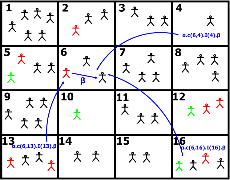
Compartmental models are often being criticized by the agent-based model researchers because they struggle to capture the connectivity between different regions of the globe, and different real-world population characteristic, such as worldwide population distribution [15] [16]. In this study, we proposed a mobility-based model, an extension to the classical SIR based epidemic model, which considers the real-world population distribution across different regions of the world. Most importantly, the model also takes into account the connectivity factor among various regions of the world, which is the key cause in accelerating the process of transforming epidemics into pandemics. We model the regions in a 2-dimensional lattice, where each cell represents the mobility parameter (or direct connectivity) from one region to another. Along with presenting the mathematical proof of our model, we have performed extensive simulations on synthetic data and forecast the COVID-19 cases in Estonia111https://koroonakaart.ee/en by inferring the interaction among individuals through call data records between Estonian counties to demonstrate the model’s ability to generalize on different types of data.
The proposed model is composed of (local) transmission rate of the infection and to cover the mobility aspect, we introduce parameters: 1) ‘’ which is a social connectivity parameter that signifies how well individuals are socially linked with each others, and 2) ‘’ that represents individuals mobility from some region to another region . Thus, the infection can transfer within the region with the transmission rate and can also be introduced from other regions through global transmission rate which depends upon , , (fraction of infected at region j) and . With the help of Figure 1, we illustrate our proposed model for better understanding. We applied our model on synthetic network as well as on a real network of Estonia considering the population density and the connectivity among counties, which is created using call data records (CDR) to investigate the following questions:
-
•
How social connectivity parameter ‘’ affects the fraction of individuals in different compartments (susceptible, infected and recovered) during a pandemic? We address this question by carefully examining the effect of while keeping all the other parameters constant (Section IV-B).
-
•
What are the outcomes of restricting mobility from the top-X percentile of strongly connected regions? We explore the outcomes of mobility restriction with the model and found that restricting the mobility of top-10 percentile of connected regions can reduce the number of infected individuals between 18% to 27% (Section IV-B).
- •
-
•
How efficiently this model can perform in real scenarios? We answer this question by projecting the expected COVID-19 cases in Estonia using the model and compared the results with the real cases (Section IV-B3).
The limitation of classical compartmental epidemiological models is that they do not take into account the importance of reducing social connectivity (or isolation) and the significance of mobility restriction during the spreading of a pandemic such as COVID-19. This limitation is overcome in the proposed model. We found that the reproduction number for a pandemic depends upon the social connectivity and mobility parameter. We also discovered that during a pandemic, restricting mobility reduces the fraction of individuals in an infected compartment and reducing the social connectivity (or isolation) delays the peak and also reduces the number of infected individuals from the pandemic. We believe that this model can help to adopt a balanced strategy to address a pandemic crisis.
The rest of the paper is organized as follows. Next, we discuss related works with respect to epidemic modeling. We then describe the model preliminaries and derivations in Section III. Section IV presents the evaluation results of our model and we conclude with a discussion of future directions in Section V.
II Related Work
In this section, we discuss relevant literature with respect to epidemic modeling which involves two different lines of work. First involving agent-based modeling and the second using compartmental based modeling. In the agent-based modeling, authors model epidemics by simulating the actions and interactions of autonomous agents (both individual or collective entities such as organizations or groups) with a view of assessing their effects on the system as a whole [11] by using transportation systems such as road networks [16], airways [15] etc. These models have been used for understanding various epidemics such as smallpox [17], influenza [18], cholera [19], and very recently about COVID-19 [15].
In contrast to agent-based modeling, a differential equation based compartmental models have also been used for understanding epidemics, which is the basis of this work. This line of literature is mainly based on the classical SIR model proposed by Kermack and McKendrick [8] followed by [20] [21]. In [20], the authors considered the host population as a dynamic variable rather than constant, as conventionally assumed, which provides a broader understanding of the population behavior during infectious disease. In their work in [21], authors discuss the idea of the basic reproductive rate, threshold about host densities, and modes of transmission.
Different variations of SIR model have also been proposed to capture various real-world scenarios. For example, introducing a delay in the model to capture the incubation period during the spreading [22, 23, 24, 25] or the introduction of interventions such as antiviral drugs [26]. In a different work to represent non-linear nature of epidemic spread, a SIR rumor spreading model was proposed in which tie strengths were dependent on nodes’ degree [27]. Apart from SIR based models, there exist different flavors of compartmental models, which represent different scenarios such as SIS [13], where individuals do not recover and can become susceptible again. This model has also been studied using varying types of underlying topologies [28].
A set of works has also focused on exhibiting the epidemic spreading by using varying types of underlying network structures. For example, authors in [29], [30] and [31] used a scale-free network and in [32] a small-world evolving networks for evaluating their epidemiological framework. In their work in [33], authors combine a discrete, stochastic SEIR (E stands for exposed) model with a three-scale community network model to demonstrate that the different regional trends may be explained by different community mixing rates. A detailed study with respect to various epidemic models on varying topologies has been done in [34].
In another line of work, authors proposed models to understand epidemics based on the speed of growth. For example, in [35], authors applied their generalized-growth model to characterize the ascending phase of an outbreak on 20 different epidemics. Their findings revealed that sub-exponential growth is a common phenomenon, especially for pathogens that are not airborne. In another work [36], researchers explain the rapid spread of H1N1 in 2009 around the world by using a flexible Bayesian, space–time, Susceptible-Infected-Recovered (SIR) modeling approach. [37] developed a simulation model of a pandemic (H1N1) 2009 outbreak in a structured population using demographic data from a medium-sized city in Ontario and epidemiologic influenza pandemic data. In comparison to previous works, the proposed model introduces mobility and social connectivity parameters, the key characteristics for turning epidemics into pandemics.
| Notations | Meaning |
|---|---|
| Number of locations | |
| Connection between locations | |
| Number of susceptible individual at location at time | |
| Number of infected individual at location at time | |
| Number of recovered individual at location at time | |
| Population at location at time | |
| Social connectivity parameter | |
| Infection rate | |
| Recovery rate | |
| Individuals mobility from location to |
III Model Preliminaries And Derivations
In this section, we first explain the classical SIR model and then discuss its limitations with respect to the absence of mobility and social connectivity parameters. Next, we describe our proposed model to understand the spreading of an infection during a pandemic.
In 1926, Kermack and McKendrick [8] proposed the classical SIR model as follows:
| (1) | |||||
| (2) | |||||
| (3) |
where, , , is the fraction of susceptible, infected and recovered population at time . However, the classical SIR epidemic model does not consider the heterogeneity and topology of the real-world network. To overcome this limitation, we introduce the mobility and social connectivity parameters in our proposed model.
Let, ‘’ represents the total number of locations and ‘’ denotes the connection (or individuals’ mobility) between locations. The propagation of infection at each location is explained as: Each healthy individual can get the infection either from an infected individual located in the same location (local transmission) or from an individual visiting from other connected locations (global transmission). The local transmission rate of infection is represented by and the recovery rate as and, and [0,1]. In the next section, we discuss the local transmission of infection and then the global transmission is discussed in detail in the Section III-B.



III-A Local Transmission
Let, be the population at location i, where and the total population is divided into three compartments. The compartments for location i at time t are as follows:
-
1.
: the number of individuals susceptible or not yet infected. This compartment is referred as susceptible compartment.
-
2.
: the number of infected individuals which can further spread the disease to the individuals present in the susceptible compartment. This compartment is referred to as infected compartment.
-
3.
: the number of individuals who have been recovered from infected compartment. This compartment is referred as recovered compartment.
Our assumptions regarding the transmission of an individual from one compartment to another compartment are as follows:
-
1.
A healthy individual after becoming infected moves from susceptible to the infected compartment.
-
2.
An individual can recovered spontaneously at any time with the recovery rate . The recovery of an individual is independent of healthy and infected compartment individuals.
-
3.
Once the individual gets recovered, it will become immune to the disease and thus, will not transmit the infection to individuals in the susceptible compartment.
-
4.
In addition, this model ignores the demography that is birth or death of individuals. Therefore, the population remains constant.
III-B Global Transmission
Let, ( ) represents a set of locations, which are connected to location . Therefore, is the maximum possible number of individuals connected to location , from all the locations . The parameter reflects the mobility of individuals from locations to location . Global transmission depends upon this mobility parameter of individuals from one location to another. Similar to local transmission, is the number of individuals in infected compartment in all the locations . Hence, total mobility of infected individuals from all the other connected locations to location is .
Considering the above description, the chances of transmission of infection from all the connected locations to location is . This transmission further depends upon the social connectivity () of individuals at location . Therefore, the proportion of healthy individuals at location which can get infected from infected individuals from location is . Thus, the mean-field equations for the dynamics of the pandemic, based on the above discussed interactions:
| (4) | |||||
| (5) | |||||
| (6) |
III-C Dynamical Behaviour Of The Model
| (7) |
In order to solve mean-field Eq. (4-6), following assumptions are made (Please note that these assumptions are not considered during our experiments):
-
1.
Initially, the population at all locations is equal to N(t) at time .
-
2.
Individuals in infected compartments are equal to at all locations at time and , where, is the number of locations connected to location , that is, = .
-
3.
The mobility of individuals from one location to another location is a fraction of total population . Let, the sum of fraction of population mobility from locations is . Then, the total individuals mobility from set of locations to is . Therefore, .
| (8) | |||||
| (9) |
| (10) | |||||
| (11) | |||||
| (12) |
For simplicity, Eq. 12 can be written as:
| (13) |
Eq. 13 can be rewritten as
| (14) |
| (15) |
Solving the Eq. 15, we get
| (16) |
As pandemic arrives at steady state when hence = 0 and =
| (17) |
Let initial conditions are , = and . Therefore, Eq. 17 can be written as
| (18) |
Normalizing the Eq. 18
| (19) |
Therefore, the reproduction number is
| (20) |
In case there is no social connectivity to other locations ( or or ) then the mobility SIR model will become the standard SIR model and the reproduction number is . Therefore, the reproduction number is directly proportional to social connectivity parameter , number of connected locations and depends upon individuals’ mobility during a pandemic.
IV Evaluation
In this section, we first explain our experimental setup and next, we discuss the results of our simulation conducted using the proposed model on synthetic networks. In addition, we also applied our model for predicting the real-time Estonian COVID-19 cases.
IV-A Experimental Setup
For the analysis, we created an aggregated flow matrix of individuals per day from Origin to Destination (OD), which follows random distribution. Furthermore, three different techniques are considered for selecting the seed infection location:
-
1.
Pandemics origin from a random location: In this, a random location is selected as seed infection location and a small fraction of individuals were infected at that location.
-
2.
Pandemics origin from a weakly connected location: Here, seed location is selected strategically, which is weakly connected to other locations. That implies least mobility of individuals from this location to other locations.
-
3.
Pandemics origin from a strongly connected location: In this also, seed location is selected strategically, which is strongly connected to other locations. This signifies that, highest mobility of individuals from this location to other locations.
Our simulation is oriented towards addressing the following questions:
-
•
How social connectivity parameter ‘’ affects the fraction of individuals in different compartments (susceptible, infected and recovered) during a pandemic?
-
•
What are the outcomes of restricting the mobility (for top-X percentile) of strongly connected locations?
-
•
What is the relationship between social connectivity parameter ‘’ and the mobility restriction (top-X percentile of strongly connected locations?
-
•
How efficiently this model can perform in real scenarios? We answer this question by projecting the expected COVID-19 cases in Estonia.
IV-B Results
We perform various simulation experiments to explain the proposed model on OD network by using previously discussed techniques for selecting the seed infection location. It is to be noted that, if , then the model will behave as a standard SIR model. Also, if the mobility is reduced to 100 percentile (that is no mobility allowed) from strongly connected locations, then also model will act as a standard SIR model.
IV-B1 Pandemics Origin From a Random Location
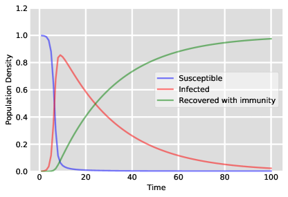
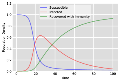
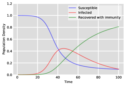
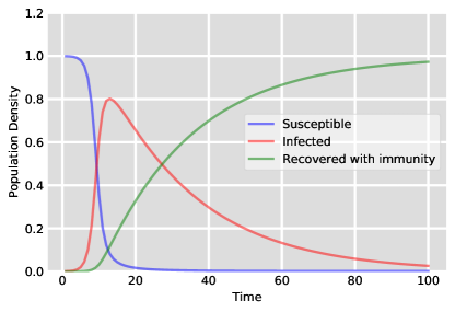
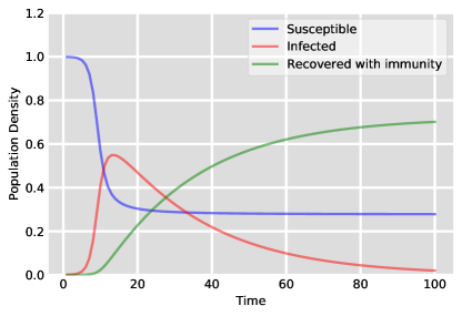
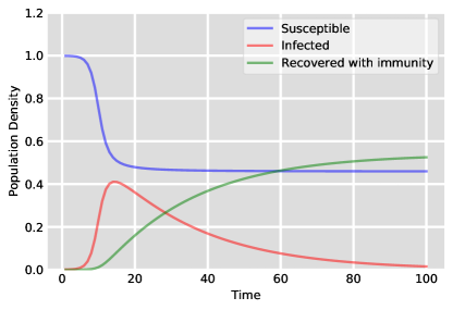
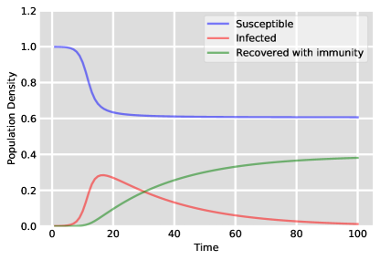
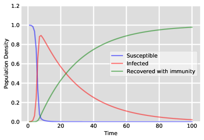
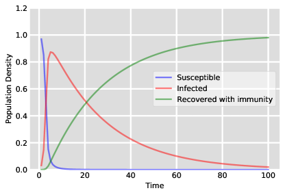
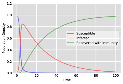
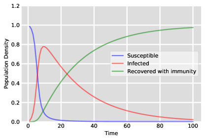
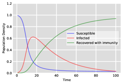
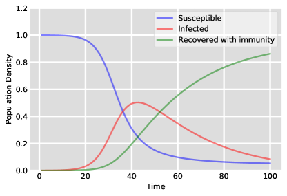
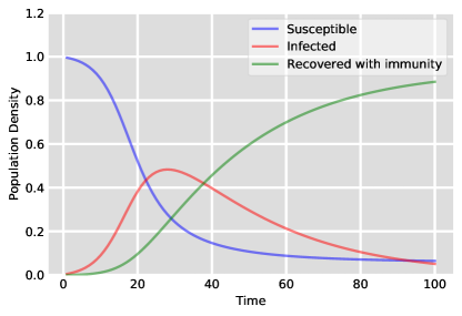
Fig. 2 displays the influence of the social connectivity parameter ’’ while retaining the other parameters constant. Fig. 2a to 2f shows the pandemic dynamics with different values of starting with to . We observe that the peak of the infected compartment decreases significantly, as the decreases, and it also takes longer to reach its peak. This indicates that there is a positive impact of lock-down in controlling a pandemic.
The effect of restricting the mobility from the top-X percentile of highly connected locations with other locations is shown in Fig. 3. Fig. 3a to 3d displays the pandemic dynamics with different percentile of mobility restrictions of highly connected locations starting with 0% to 30% (keeping ). We observe that in case of pandemic, restricting the mobility from the top-10 percentile of highly connected locations can reduce the number of individuals who can get infected to 27%. Therefore, quarantine plays a vital role during pandemics.
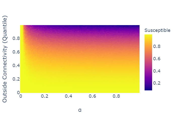
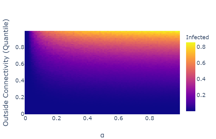
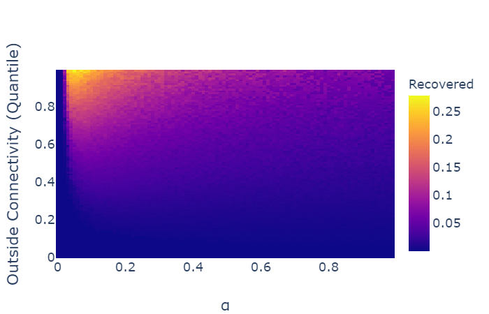
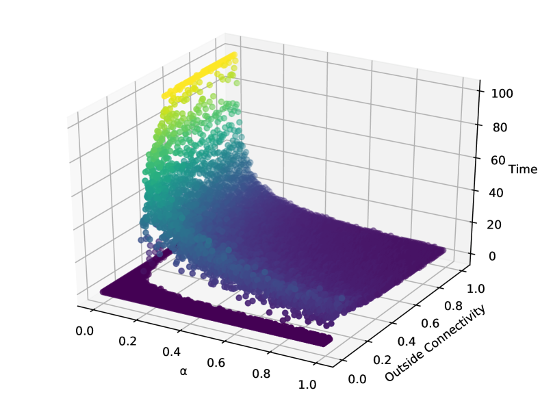
In order to understand the relationship between and mobility restriction from strongly connected locations, we performed the numerical simulation of the proposed mean-field equations (see Figure 4). We can infer that social connectivity parameter ‘’ and mobility both plays an important role during pandemics. Therefore, it is advisable to follow a dual strategy approach during a pandemic outbreak as controlling mobility reduces the fraction of infected individuals and delays the peak. Furthermore, we analysed the number of days required to reach the point where highest fraction of individuals get infected (see Figure 5). This indicates that mobility restrictions and minimal social contact will postpone the pandemic’s peak and will give sufficient time for the preparations especially for the health sector.
IV-B2 Pandemics Origin From a Weakly and Strongly Connected Locations
Fig. 6 displays the influence of the social communication parameter ’’ while keeping the other parameters constant for both weakly and strongly connected locations. Fig. 6a to 6l shows the pandemic dynamics with different values of starting with to .
It can be noted that when a pandemic originates from a weakly connected location, it takes longer to reach its peak compared to when it starts from a strongly connected location. This shows that location of origin also plays an important role during pandemic. Similar to random location, reducing mobility from the highly connected locations by 10 percentile can reduce the number of infected individuals between 18% to 27% for weakly and strongly connected locations.
IV-B3 Case Study Of Estonia
To demonstrate the usability of the model, we applied it on a real-time data of Estonia’s to fit COVID-19 cases. Fig. 7 shows the actual number of cases and the cases forecast by the model using different values for and mobility percentile. For example, when , this indicates that social connectivity of individuals are reduced by 5% and also top-5% of strongly connected locations are restricted from mobility. Similarly, , implies that social connectivity of individuals are reduced by 30% and also the top-30% of strongly connected locations have introduced restricted mobility.
For simulation, we created the matrix between counties of Estonia using call data records [38]. Furthermore, these call interactions are converted into population mobility between counties using Estonian population data [39]. For the local transmission of the virus (within the county), we consider the reproduction number [40].




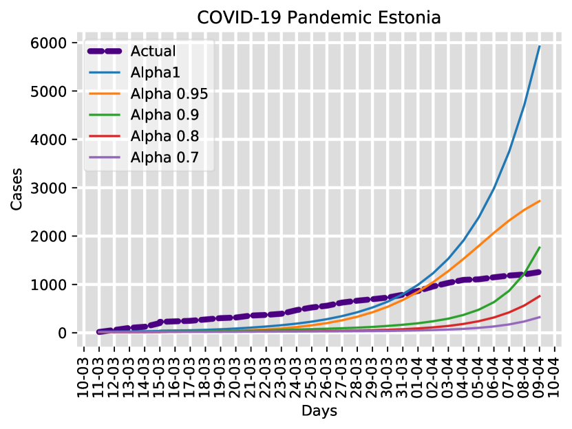
Cases reported until March, 2020 are considered as initial condition for the model. The reason behind selecting March, 2020 as initial condition is that, till this date no local transmission of the virus was reported222https://www.err.ee/1063204/terviseamet-eestis-on-kinnitatud-27-koroonajuhtu-ja-kohalik-levik. Till the day of initial condition, the Estonian Health Board confirmed 13 cases in Harju and two cases in Tartumaa and Saaremaa each333https://www.terviseamet.ee/et/uuskoroonaviirus. During the simulation, the number of cases in all other counties are initialized to zero. The infection rate and recovery rate are adjusted according to the value of for COVID-19. By April 2020, reported cases in Estonia and forecast cases using the model are shown in Fig. 7. It can be noticed that the model predicted much higher cases of COVID-19 if no restrictions are introduced ( = 1). However, as the restrictions were introduced by the Government444https://www.valitsus.ee/en/news the number of cases got damped (Actual). Thus, the applicability of this model is to forecast a range of predicted number of cases which can help the governmental and health agencies to understand the impact and introduce proportional interventions to restrict the spread of the epidemic.
V Conclusion
Classical compartmental epidemic models are unable to describe the spreading pattern of pandemics such as COVID-19 as they do not take into account the effect of social connectivity and mobility in spreading of the virus. Our proposed mobility based SIR model shows the significance of social connectivity and mobility during pandemics by taking into consideration the local and the global transmission rate of the infection. We have simulated the proposed model considering three different origins of the infection, namely random location, weakly connected location and strongly connected location. Our simulation shows that limiting the social connectivity reduces and delays the peak of the infected compartment. Our analysis also shows that restricting the mobility from the top-10 percentile of connected locations can reduce the number of infected individuals between 18% to 27%. From the mathematical proof for our proposed model, we obtained that the reproduction number directly depends upon social connectivity of individuals, number of connected locations and individuals mobility between locations which is in line with our simulations’ results. This indicates that introducing isolation and quarantine is effective in fighting a pandemic crisis. Using the proposed model, we also simulated the real world scenario by considering the COVID-19 cases in Estonia. Simulation reveals that the mobility based SIR model can be helpful to forecast the expected number of cases after some proportion of isolation and quarantine is introduced in the society.
We plan to include various future directions for this work such as by simulating the model using additional dynamic networks. Another direction would be to use additional mobility data such as transportation network for better understanding the pandemic behavior. Importantly, we plan to introduce infection delay and recovery delay simultaneously in our future studies.
Acknowledgment
This research was funded by ERDF via the IT Academy Research Programme and SoBigData++.
References
- [1] W. H. Organization et al., “Pandemic h1n1 2009,” WHO Regional Office for South-East Asia, Tech. Rep., 2009.
- [2] C. for Disease Control, Prevention et al., “First global estimates of 2009 h1n1 pandemic mortality released by cdc-led collaboration. 2012.”
- [3] J. CSSE, “Coronavirus covid-19 global cases by the center for systems science and engineering (csse) at johns hopkins university (jhu),” 2020.
- [4] C. COVID, “Global cases by the center for systems science and engineering (csse) at johns hopkins university (jhu),” 19.
- [5] E. Bonabeau, “Agent-based modeling: Methods and techniques for simulating human systems,” Proceedings of the national academy of sciences, vol. 99, no. suppl 3, pp. 7280–7287, 2002.
- [6] T. C. Schelling, “Dynamic models of segregation,” Journal of mathematical sociology, vol. 1, no. 2, pp. 143–186, 1971.
- [7] R. Sun et al., Cognition and multi-agent interaction: From cognitive modeling to social simulation. Cambridge University Press, 2006.
- [8] W. O. Kermack and A. G. McKendrick, “A contribution to the mathematical theory of epidemics,” in Proceedings of the Royal Society of London A: mathematical, physical and engineering sciences, vol. 115, no. 772. The Royal Society, 1927, pp. 700–721.
- [9] H. W. Hethcote, “The mathematics of infectious diseases,” SIAM review, vol. 42, no. 4, pp. 599–653, 2000.
- [10] R. Goel, A. Singh, and F. Ghanbarnejad, “Modeling competitive marketing strategies in social networks,” Physica A: Statistical Mechanics and its Applications, vol. 518, pp. 50–70, 2019.
- [11] J. M. Epstein, “Modelling to contain pandemics,” Nature, vol. 460, no. 7256, pp. 687–687, 2009.
- [12] M. Hurley, G. Jacobs, and M. Gilbert, “The basic si model,” New Directions for Teaching and Learning, vol. 2006, no. 106, pp. 11–22, 2006.
- [13] I. Nåsell, “The quasi-stationary distribution of the closed endemic sis model,” Advances in Applied Probability, vol. 28, no. 3, pp. 895–932, 1996.
- [14] Y. Jin, W. Wang, and S. Xiao, “An sirs model with a nonlinear incidence rate,” Chaos, Solitons & Fractals, vol. 34, no. 5, pp. 1482–1497, 2007.
- [15] M. Chinazzi, J. T. Davis, M. Ajelli, C. Gioannini, M. Litvinova, S. Merler, A. P. y Piontti, K. Mu, L. Rossi, K. Sun et al., “The effect of travel restrictions on the spread of the 2019 novel coronavirus (covid-19) outbreak,” Science, 2020.
- [16] S. Eubank, H. Guclu, V. A. Kumar, M. V. Marathe, A. Srinivasan, Z. Toroczkai, and N. Wang, “Modelling disease outbreaks in realistic urban social networks,” Nature, vol. 429, no. 6988, pp. 180–184, 2004.
- [17] D. S. Burke, J. M. Epstein, D. A. Cummings, J. I. Parker, K. C. Cline, R. M. Singa, and S. Chakravarty, “Individual-based computational modeling of smallpox epidemic control strategies,” Academic Emergency Medicine, vol. 13, no. 11, pp. 1142–1149, 2006.
- [18] K. M. Khalil, M. Abdel-Aziz, T. T. Nazmy, and A.-B. M. Salem, “An agent-based modeling for pandemic influenza in egypt,” in Handbook on Decision Making. Springer, 2012, pp. 205–218.
- [19] A. T. Crooks and A. B. Hailegiorgis, “An agent-based modeling approach applied to the spread of cholera,” Environmental Modelling & Software, vol. 62, pp. 164–177, 2014.
- [20] R. M. Anderson and R. M. May, “Population biology of infectious diseases: Part i,” Nature, vol. 280, no. 5721, p. 361, 1979.
- [21] R. M. Anderson, R. M. May, and B. Anderson, Infectious diseases of humans: dynamics and control. Wiley Online Library, 1992, vol. 28.
- [22] J.-Z. Zhang, J.-J. Wang, T.-X. Su, and Z. Jin, “Analysis of a delayed sir epidemic model,” in Computational Aspects of Social Networks (CASoN), 2010 International Conference on. IEEE, 2010, pp. 192–195.
- [23] C. Xia, L. Wang, S. Sun, and J. Wang, “An sir model with infection delay and propagation vector in complex networks,” Nonlinear Dynamics, vol. 69, no. 3, pp. 927–934, 2012.
- [24] L. Liu, “A delayed sir model with general nonlinear incidence rate,” Advances in Difference Equations, vol. 2015, no. 1, p. 329, 2015.
- [25] M. Arquam, A. Singh, and R. Sharma, “Modelling and analysis of delayed sir model on complex network,” in International Conference on Complex Networks and their Applications. Springer, 2018, pp. 418–430.
- [26] S. Towers, K. V. Geisse, Y. Zheng, and Z. Feng, “Antiviral treatment for pandemic influenza: Assessing potential repercussions using a seasonally forced sir model,” Journal of theoretical biology, vol. 289, pp. 259–268, 2011.
- [27] A. Singh and Y. N. Singh, “Nonlinear spread of rumor and inoculation strategies in the nodes with degree dependent tie strength in complex networks,” arXiv preprint arXiv:1208.6063, 2012.
- [28] H. Shi, Z. Duan, and G. Chen, “An sis model with infective medium on complex networks,” Physica A: Statistical Mechanics and its Applications, vol. 387, no. 8-9, pp. 2133–2144, 2008.
- [29] Y. Moreno, R. Pastor-Satorras, and A. Vespignani, “Epidemic outbreaks in complex heterogeneous networks,” The European Physical Journal B-Condensed Matter and Complex Systems, vol. 26, no. 4, pp. 521–529, 2002.
- [30] M. Barthélemy, A. Barrat, R. Pastor-Satorras, and A. Vespignani, “Dynamical patterns of epidemic outbreaks in complex heterogeneous networks,” Journal of theoretical biology, vol. 235, no. 2, pp. 275–288, 2005.
- [31] A. Vespignani, “Modelling dynamical processes in complex socio-technical systems,” Nature physics, vol. 8, no. 1, p. 32, 2012.
- [32] X. Li and X. Wang, “Controlling the spreading in small-world evolving networks: stability, oscillation, and topology,” IEEE Transactions on Automatic Control, vol. 51, no. 3, pp. 534–540, 2006.
- [33] M. A. Kiskowski, “A three-scale network model for the early growth dynamics of 2014 west africa ebola epidemic,” PLoS currents, vol. 6, 2014.
- [34] R. Pastor-Satorras, C. Castellano, P. Van Mieghem, and A. Vespignani, “Epidemic processes in complex networks,” Reviews of modern physics, vol. 87, no. 3, p. 925, 2015.
- [35] C. Viboud, L. Simonsen, and G. Chowell, “A generalized-growth model to characterize the early ascending phase of infectious disease outbreaks,” Epidemics, vol. 15, pp. 27–37, 2016.
- [36] X. Huang, A. C. Clements, G. Williams, K. Mengersen, S. Tong, and W. Hu, “Bayesian estimation of the dynamics of pandemic (h1n1) 2009 influenza transmission in queensland: A space–time sir-based model,” Environmental research, vol. 146, pp. 308–314, 2016.
- [37] M. Z. Gojovic, B. Sander, D. Fisman, M. D. Krahn, and C. T. Bauch, “Modelling mitigation strategies for pandemic (h1n1) 2009,” Cmaj, vol. 181, no. 10, pp. 673–680, 2009.
- [38] H. Hiir, R. Sharma, A. Aasa, and E. Saluveer, “Impact of natural and social events on mobile call data records–an estonian case study,” in International Conference on Complex Networks and Their Applications. Springer, 2019, pp. 415–426.
- [39] S. Estonia, “Quarterly bulletin of statistics estonia,” 2018.
- [40] W. H. Organization et al., “Coronavirus disease 2019 ( covid-19): situation report, 46,” 2020.