DeeBERT: Dynamic Early Exiting for Accelerating BERT Inference
Abstract
Large-scale pre-trained language models such as BERT have brought significant improvements to NLP applications. However, they are also notorious for being slow in inference, which makes them difficult to deploy in real-time applications. We propose a simple but effective method, DeeBERT, to accelerate BERT inference. Our approach allows samples to exit earlier without passing through the entire model. Experiments show that DeeBERT is able to save up to 40% inference time with minimal degradation in model quality. Further analyses show different behaviors in the BERT transformer layers and also reveal their redundancy. Our work provides new ideas to efficiently apply deep transformer-based models to downstream tasks. Code is available at https://github.com/castorini/DeeBERT.
1 Introduction
Large-scale pre-trained language models such as ELMo Peters et al. (2018), GPT Radford et al. (2019), BERT Devlin et al. (2019), XLNet Yang et al. (2019), and RoBERTa Liu et al. (2019) have brought significant improvements to natural language processing (NLP) applications. Despite their power, they are notorious for being enormous in size and slow in both training and inference. Their long inference latencies present challenges to deployment in real-time applications and hardware-constrained edge devices such as mobile phones and smart watches.
To accelerate inference for BERT, we propose DeeBERT: Dynamic early exiting for BERT. The inspiration comes from a well-known observation in the computer vision community: in deep convolutional neural networks, higher layers typically produce more detailed and finer-grained features Zeiler and Fergus (2014). Therefore, we hypothesize that, for BERT, features provided by the intermediate transformer layers may suffice to classify some input samples.

DeeBERT accelerates BERT inference by inserting extra classification layers (which we refer to as off-ramps) between each transformer layer of BERT (Figure 1). All transformer layers and off-ramps are jointly fine-tuned on a given downstream dataset. At inference time, after a sample goes through a transformer layer, it is passed to the following off-ramp. If the off-ramp is confident of the prediction, the result is returned; otherwise, the sample is sent to the next transformer layer.
In this paper, we conduct experiments on BERT and RoBERTa with six GLUE datasets, showing that DeeBERT is capable of accelerating model inference by up to 40% with minimal model quality degradation on downstream tasks. Further analyses reveal interesting patterns in the models’ transformer layers, as well as redundancy in both BERT and RoBERTa.
2 Related Work
BERT and RoBERTa are large-scale pre-trained language models based on transformers Vaswani et al. (2017). Despite their groundbreaking power, there have been many papers trying to examine and exploit their over-parameterization. Michel et al. (2019) and Voita et al. (2019) analyze redundancy in attention heads. Q-BERT Shen et al. (2019) uses quantization to compress BERT, and LayerDrop Fan et al. (2019) uses group regularization to enable structured pruning at inference time. On the knowledge distillation side, TinyBERT Jiao et al. (2019) and DistilBERT Sanh et al. (2019) both distill BERT into a smaller transformer-based model, and Tang et al. (2019) distill BERT into even smaller non-transformer-based models.
Our work is inspired by Cambazoglu et al. (2010), Teerapittayanon et al. (2017), and Huang et al. (2018), but mainly differs from previous work in that we focus on improving model efficiency with minimal quality degradation.
| SST-2 | MRPC | QNLI | RTE | QQP | MNLI-(m/mm) | |||||||
| Acc | Time | F1 | Time | Acc | Time | Acc | Time | F1 | Time | Acc | Time | |
| BERT-base | ||||||||||||
| Baseline | 93.6 | 36.72s | 88.2 | 34.77s | 91.0 | 111.44s | 69.9 | 61.26s | 71.4 | 145min | 83.9/83.0 | 202.84s |
| DistilBERT | 1.4 | 40% | 1.1 | 40% | 2.6 | 40% | 9.4 | 40% | 1.1 | 40% | 4.5 | 40% |
| DeeBERT | 0.2 | 21% | 0.3 | 14% | 0.1 | 15% | 0.4 | 9% | 0.0 | 24% | 0.0/0.1 | 14% |
| 0.6 | 40% | 1.3 | 31% | 0.7 | 29% | 0.6 | 11% | 0.1 | 39% | 0.8/0.7 | 25% | |
| 2.1 | 47% | 3.0 | 44% | 3.1 | 44% | 3.2 | 33% | 2.0 | 49% | 3.9/3.8 | 37% | |
| RoBERTa-base | ||||||||||||
| Baseline | 94.3 | 36.73s | 90.4 | 35.24s | 92.4 | 112.96s | 67.5 | 60.14s | 71.8 | 152min | 87.0/86.3 | 198.52s |
| LayerDrop | 1.8 | 50% | - | - | - | - | - | - | - | - | 4.1 | 50% |
| DeeBERT | 0.1 | 26% | 0.1 | 25% | 0.1 | 25% | 0.6 | 32% | 0.1 | 32% | 0.0/0.0 | 19% |
| 0.0 | 33% | 0.2 | 28% | 0.5 | 30% | 0.4 | 33% | 0.0 | 39% | 0.1/0.3 | 23% | |
| 1.8 | 44% | 1.1 | 38% | 2.5 | 39% | 1.1 | 35% | 0.6 | 44% | 3.9/4.1 | 29% | |
3 Early Exit for BERT inference
DeeBERT modifies fine-tuning and inference of BERT models, leaving pre-training unchanged. It adds one off-ramp for each transformer layer. An inference sample can exit earlier at an off-ramp, without going through the rest of the transformer layers. The last off-ramp is the classification layer of the original BERT model.
3.1 DeeBERT at Fine-Tuning
We start with a pre-trained BERT model with transformer layers and add off-ramps to it. For fine-tuning on a downstream task, the loss function of the off-ramp is
| (1) |
where is the fine-tuning training set, is the collection of all parameters, is the feature–label pair of a sample, is the cross-entropy loss function, and is the output of the off-ramp.
The network is fine-tuned in two stages:
-
1.
Update the embedding layer, all transformer layers, and the last off-ramp with the loss function . This stage is identical to BERT fine-tuning in the original paper Devlin et al. (2019).
-
2.
Freeze all parameters fine-tuned in the first stage, and then update all but the last off-ramp with the loss function . The reason for freezing parameters of transformer layers is to keep the optimal output quality for the last off-ramp; otherwise, transformer layers are no longer optimized solely for the last off-ramp, generally worsening its quality.
3.2 DeeBERT at Inference
The way DeeBERT works at inference time is shown in Algorithm 1. We quantify an off-ramp’s confidence in its prediction using the entropy of the output probability distribution . When an input sample arrives at an off-ramp, the off-ramp compares the entropy of its output distribution with a preset threshold to determine whether the sample should be returned here or sent to the next transformer layer.
It is clear from both intuition and experimentation that a larger leads to a faster but less accurate model, and a smaller leads to a more accurate but slower one. In our experiments, we choose based on this principle.
We also explored using ensembles of multiple layers instead of a single layer for the off-ramp, but this does not bring significant improvements. The reason is that predictions from different layers are usually highly correlated, and a wrong prediction is unlikely to be “fixed” by the other layers. Therefore, we stick to the simple yet efficient single output layer strategy.
4 Experiments
4.1 Experimental Setup
We apply DeeBERT to both BERT and RoBERTa, and conduct experiments on six classification datasets from the GLUE benchmark Wang et al. (2018): SST-2, MRPC, QNLI, RTE, QQP, and MNLI. Our implementation of DeeBERT is adapted from the HuggingFace Transformers Library Wolf et al. (2019). Inference runtime measurements are performed on a single NVIDIA Tesla P100 graphics card. Hyperparameters such as hidden-state size, learning rate, fine-tune epoch, and batch size are kept unchanged from the library. There is no early stopping and the checkpoint after full fine-tuning is chosen.
4.2 Main Results
We vary DeeBERT’s quality–efficiency trade-off by setting different entropy thresholds , and compare the results with other baselines in Table 1. Model quality is measured on the test set, and the results are provided by the GLUE evaluation server. Efficiency is quantified with wall-clock inference runtime111This includes both CPU and GPU runtime. on the entire test set, where samples are fed into the model one by one. For each run of DeeBERT on a dataset, we choose three entropy thresholds based on quality–efficiency trade-offs on the development set, aiming to demonstrate two cases: (1) the maximum runtime savings with minimal performance drop (), and (2) the runtime savings with moderate performance drop (). Chosen values differ for each dataset.
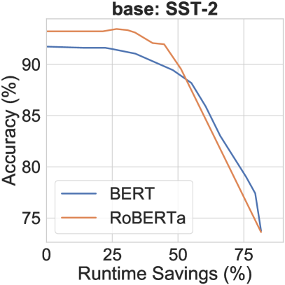
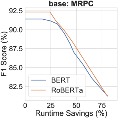
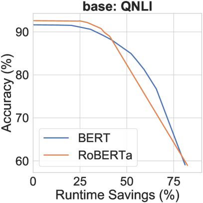
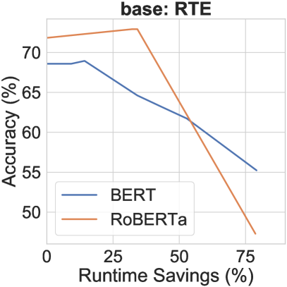
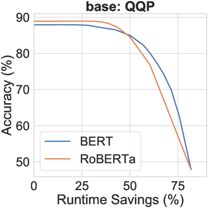
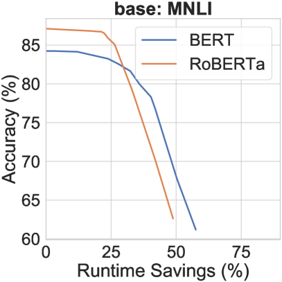
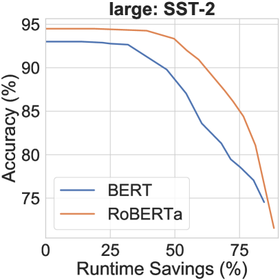
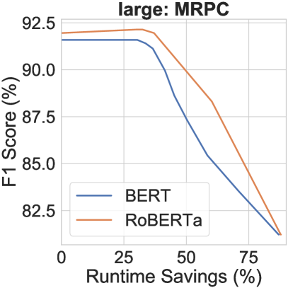
We also visualize the trade-off in Figure 2. Each curve is drawn by interpolating a number of points, each of which corresponds to a different threshold . Since this only involves a comparison between different settings of DeeBERT, runtime is measured on the development set.
-
•
Despite differences in baseline performance, both models show similar patterns on all datasets: the performance (accuracy/F1 score) stays (mostly) the same until runtime saving reaches a certain turning point, and then starts to drop gradually. The turning point typically comes earlier for BERT than for RoBERTa, but after the turning point, the performance of RoBERTa drops faster than for BERT. The reason for this will be discussed in Section 4.4.
-
•
Occasionally, we observe spikes in the curves, e.g., RoBERTa in SST-2, and both BERT and RoBERTa in RTE. We attribute this to possible regularization brought by early exiting and thus smaller effective model sizes, i.e., in some cases, using all transformer layers may not be as good as using only some of them.
Compared with other BERT acceleration methods, DeeBERT has the following two advantages:
-
•
Instead of producing a fixed-size smaller model like DistilBERT Sanh et al. (2019), DeeBERT produces a series of options for faster inference, which users have the flexibility to choose from, according to their demands.
-
•
Unlike DistilBERT and LayerDrop Fan et al. (2019), DeeBERT does not require further pre-training of the transformer model, which is much more time-consuming than fine-tuning.
4.3 Expected Savings
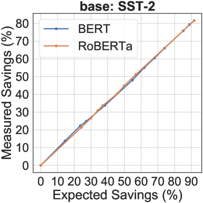
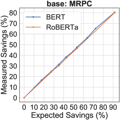
As the measurement of runtime might not be stable, we propose another metric to capture efficiency, called expected saving, defined as
| (2) |
where is the number of layers and is the number of samples exiting at layer . Intuitively, expected saving is the fraction of transformer layer execution saved by using early exiting. The advantage of this metric is that it remains invariant between different runs and can be analytically computed. For validation, we compare this metric with measured saving in Figure 3. Overall, the curves show a linear relationship between expected savings and measured savings, indicating that our reported runtime is a stable measurement of DeeBERT’s efficiency.
4.4 Layerwise Analyses
In order to understand the effect of applying DeeBERT to both models, we conduct further analyses on each off-ramp layer. Experiments in this section are also performed on the development set.
Output Performance by Layer.
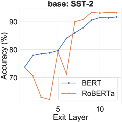
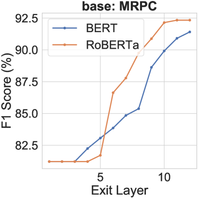
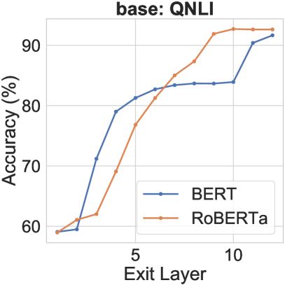
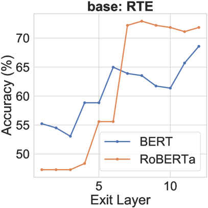
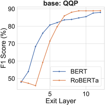
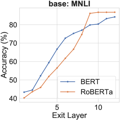
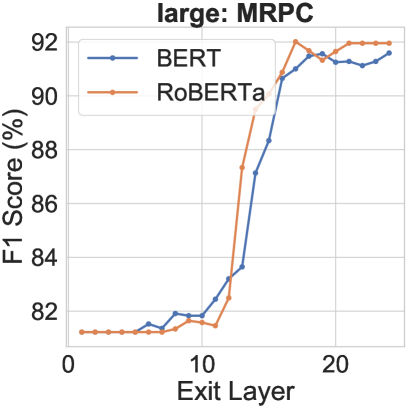
For each off-ramp, we force all samples in the development set to exit here, measure the output quality, and visualize the results in Figure 4.
From the figure, we notice the difference between BERT and RoBERTa. The output quality of BERT improves at a relatively stable rate as the index of the exit off-ramp increases. The output quality of RoBERTa, on the other hand, stays almost unchanged (or even worsens) for a few layers, then rapidly improves, and reaches a saturation point before BERT does. This provides an explanation for the phenomenon mentioned in Section 4.2: on the same dataset, RoBERTa often achieves more runtime savings while maintaining roughly the same output quality, but then quality drops faster after reaching the turning point.
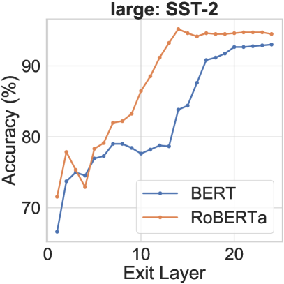
We also show the results for BERT-large and RoBERTa-large in Figure 5. From the two plots on the right, we observe signs of redundancy that both BERT-large and RoBERTa-large share: the last several layers do not show much improvement compared with the previous layers (performance even drops slightly in some cases). Such redundancy can also be seen in Figure 4.
Number of Exiting Samples by Layer.
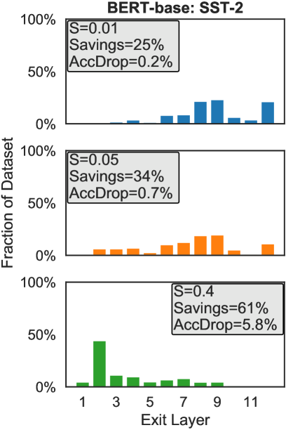
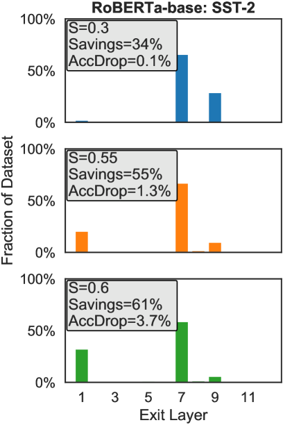
We further show the fraction of samples exiting at each off-ramp for a given entropy threshold in Figure 6.
Entropy threshold is the baseline, and all samples exit at the last layer; as increases, gradually more samples exit earlier. Apart from the obvious, we observe additional, interesting patterns: if a layer does not provide better-quality output than previous layers, such as layer 11 in BERT-base and layers 2–4 and 6 in RoBERTa-base (which can be seen in Figure 4, top left), it is typically chosen by very few samples; popular layers are typically those that substantially improve over previous layers, such as layer 7 and 9 in RoBERTa-base. This shows that an entropy threshold is able to choose the fastest off-ramp among those with comparable quality, and achieves a good trade-off between quality and efficiency.
5 Conclusions and Future Work
We propose DeeBERT, an effective method that exploits redundancy in BERT models to achieve better quality–efficiency trade-offs. Experiments demonstrate its ability to accelerate BERT’s and RoBERTa’s inference by up to 40%, and also reveal interesting patterns of different transformer layers in BERT models.
There are a few interesting questions left unanswered in this paper, which would provide interesting future research directions: (1) DeeBERT’s training method, while maintaining good quality in the last off-ramp, reduces model capacity available for intermediate off-ramps; it would be important to look for a method that achieves a better balance between all off-ramps. (2) The reasons why some transformer layers appear redundant222For example, the first and last four layers of RoBERTa-base on SST-2 (Figure 4, top left). and why DeeBERT considers some samples easier than others remain unknown; it would be interesting to further explore relationships between pre-training and layer redundancy, sample complexity and exit layer, and related characteristics.
Acknowledgment
We thank anonymous reviewers for their insightful suggestions. We also gratefully acknowledge funding support from the Natural Sciences and Engineering Research Council (NSERC) of Canada. Computational resources used in this work were provided, in part, by the Province of Ontario, the Government of Canada through CIFAR, and companies sponsoring the Vector Institute.
References
- Cambazoglu et al. (2010) B. Barla Cambazoglu, Hugo Zaragoza, Olivier Chapelle, Jiang Chen, Ciya Liao, Zhaohui Zheng, and Jon Degenhardt. 2010. Early exit optimizations for additive machine learned ranking systems. In Proceedings of the Third ACM International Conference on Web Search and Data Mining (WSDM 2010), pages 411–420, New York, New York.
- Devlin et al. (2019) Jacob Devlin, Ming-Wei Chang, Kenton Lee, and Kristina Toutanova. 2019. BERT: Pre-training of deep bidirectional transformers for language understanding. In Proceedings of the 2019 Conference of the North American Chapter of the Association for Computational Linguistics: Human Language Technologies, Volume 1 (Long and Short Papers), pages 4171–4186, Minneapolis, Minnesota.
- Fan et al. (2019) Angela Fan, Edouard Grave, and Armand Joulin. 2019. Reducing transformer depth on demand with structured dropout. arXiv:1909.11556.
- Huang et al. (2018) Gao Huang, Danlu Chen, Tianhong Li, Felix Wu, Laurens van der Maaten, and Kilian Weinberger. 2018. Multi-scale dense networks for resource efficient image classification. In Proceedings of the 6th International Conference on Learning Representations, Vancouver, BC, Canada.
- Jiao et al. (2019) Xiaoqi Jiao, Yichun Yin, Lifeng Shang, Xin Jiang, Xiao Chen, Linlin Li, Fang Wang, and Qun Liu. 2019. TinyBERT: Distilling BERT for natural language understanding. arXiv:1909.10351.
- Liu et al. (2019) Yinhan Liu, Myle Ott, Naman Goyal, Jingfei Du, Mandar Joshi, Danqi Chen, Omer Levy, Mike Lewis, Luke Zettlemoyer, and Veselin Stoyanov. 2019. RoBERTa: A robustly optimized BERT pretraining approach. arXiv:1907.11692.
- Michel et al. (2019) Paul Michel, Omer Levy, and Graham Neubig. 2019. Are sixteen heads really better than one? In Advances in Neural Information Processing Systems 32, pages 14014–14024.
- Peters et al. (2018) Matthew Peters, Mark Neumann, Mohit Iyyer, Matt Gardner, Christopher Clark, Kenton Lee, and Luke Zettlemoyer. 2018. Deep contextualized word representations. In Proceedings of the 2018 Conference of the North American Chapter of the Association for Computational Linguistics: Human Language Technologies, Volume 1 (Long Papers), pages 2227–2237, New Orleans, Louisiana.
- Radford et al. (2019) Alec Radford, Jeffrey Wu, Rewon Child, David Luan, Dario Amodei, and Ilya Sutskever. 2019. Language models are unsupervised multitask learners. OpenAI Blog.
- Sanh et al. (2019) Victor Sanh, Lysandre Debut, Julien Chaumond, and Thomas Wolf. 2019. DistilBERT, a distilled version of BERT: smaller, faster, cheaper and lighter. arXiv:1910.01108.
- Shen et al. (2019) Sheng Shen, Zhen Dong, Jiayu Ye, Linjian Ma, Zhewei Yao, Amir Gholami, Michael W. Mahoney, and Kurt Keutzer. 2019. Q-BERT: Hessian based ultra low precision quantization of BERT. arXiv:1909.05840.
- Tang et al. (2019) Raphael Tang, Yao Lu, and Jimmy Lin. 2019. Natural language generation for effective knowledge distillation. In Proceedings of the 2nd Workshop on Deep Learning Approaches for Low-Resource NLP (DeepLo 2019), pages 202–208, Hong Kong, China.
- Teerapittayanon et al. (2017) Surat Teerapittayanon, Bradley McDanel, and Hsiang-Tsung Kung. 2017. BranchyNet: Fast inference via early exiting from deep neural networks. arXiv:1709.01686.
- Vaswani et al. (2017) Ashish Vaswani, Noam Shazeer, Niki Parmar, Jakob Uszkoreit, Llion Jones, Aidan N. Gomez, Łukasz Kaiser, and Illia Polosukhin. 2017. Attention is all you need. In Advances in Neural Information Processing Systems 30, pages 5998–6008.
- Voita et al. (2019) Elena Voita, David Talbot, Fedor Moiseev, Rico Sennrich, and Ivan Titov. 2019. Analyzing multi-head self-attention: Specialized heads do the heavy lifting, the rest can be pruned. In Proceedings of the 57th Annual Meeting of the Association for Computational Linguistics, pages 5797–5808, Florence, Italy.
- Wang et al. (2018) Alex Wang, Amanpreet Singh, Julian Michael, Felix Hill, Omer Levy, and Samuel Bowman. 2018. GLUE: A multi-task benchmark and analysis platform for natural language understanding. In Proceedings of the 2018 EMNLP Workshop BlackboxNLP: Analyzing and Interpreting Neural Networks for NLP, pages 353–355, Brussels, Belgium.
- Wolf et al. (2019) Thomas Wolf, Lysandre Debut, Victor Sanh, Julien Chaumond, Clement Delangue, Anthony Moi, Pierric Cistac, Tim Rault, R’emi Louf, Morgan Funtowicz, and Jamie Brew. 2019. HuggingFace’s Transformers: State-of-the-art natural language processing. arXiv:1910.03771.
- Yang et al. (2019) Zhilin Yang, Zihang Dai, Yiming Yang, Jaime G. Carbonell, Ruslan Salakhutdinov, and Quoc V. Le. 2019. XLNet: generalized autoregressive pretraining for language understanding. arXiv:1906.08237.
- Zeiler and Fergus (2014) Matthew D. Zeiler and Rob Fergus. 2014. Visualizing and understanding convolutional networks. In Proceedings of the 13th European Conference on Computer Vision (ECCV 2014), pages 818–833, Zürich, Switzerland.