Evolutionary Stochastic Policy Distillation
Abstract
Solving the Goal-Conditioned Reward Sparse (GCRS) task is a challenging reinforcement learning problem due to the sparsity of reward signals. In this work, we propose a new formulation of GCRS tasks from the perspective of the drifted random walk on the state space. Based on the formulation we design a novel method called Evolutionary Stochastic Policy Distillation (ESPD) to solve GCRS tasks by reducing the First Hitting Time of the stochastic process. As a self-imitate approach, ESPD learns a target policy efficiently from a series of its stochastic variants in a supervised learning manner. ESPD follows an Evolution Strategy that applies perturbations upon the action of the target policy as the behavior policy for generating experiences and then select the experiences of the superior stochastic variants. Finally the target policy is updated by policy distillation on the selected experience transitions. The experiments on the MuJoCo robotics control suite show the high learning efficiency of the proposed method.111Code is available at https://github.com/decisionforce/ESPD
1 Introduction
Although Reinforcement Learning (RL) has been applied to various challenging tasks and outperforms human in most cases 24, 38, 23, 44, 27, manual effort is still needed to provide sufficient learning signals beside the original Win or Loss reward signal 44. In most real-world RL tasks, the rewards are usually extremely sparse. On the one hand, such reward sparsity hinders the learning process, on the other hand, it also provides the flexibility of learning different policies as different solutions to a certain task in order to get rid of deceptive sub-optimal solutions produced by manually designed rewards 29.
Goal-Conditioned Reward Sparse (GCRS) task is one of the challenging real-world reinforcement learning tasks with extremely sparse rewards. In the task, the goal is combined with the current state as the policy input, while the agent is able to receive a positive reward only when the goal is achieved. In many cases, the GCRS task is also considered as the Multi-Goal task where the goal is not fixed and can be anywhere in the state space. Therefore the policy has to learn a general solution that can be applied to a set of similar tasks. For example, robotic object grasping is such a GCRS task: the target object could be anywhere on the table, the robot has to adjust its arm to reach the object and grasp it. The learning objective of a policy is to find a feasible path from the current state to the goal 42. Similar tasks include the Multi-Goal benchmarks in robotics control 29.
In previous works, reward shaping 26, hierarchical reinforcement learning 15, 7, curriculum learning 8 and learning from demonstrations 34, 6, 4, 21, 25 were proposed to tackle the challenges of learning through sparse rewards. These approaches provide manual guidance from different perspectives. Besides, the Hindsight Experience Replay (HER) 2, 3 was proposed to relabel failed trajectories and assign hindsight credits as complementary to the primal sparse rewards, which is still a kind of Temporal Difference learning and relies on the value of reward. Recently the Policy Continuation with Hindsight Inverse Dynamics (PCHID) 40 is proposed to learn with hindsight experiences in a supervised learning manner, but the learning efficiency is still limited by the explicit curriculum setting.
In this work, we intend to further improve the learning efficiency and stability for these GCRS tasks with an alternative approach based on supervised learning. Specifically, by formulating the exploration in GCRS tasks as a random walk in the state space, solving the GCRS task is then equivalent to decreasing the first hitting time (FHT) in the random walk. The main idea of our method is encouraging the policy to reproduce trajectories that have shorter FHTs. With such a self-imitated manner, the policy learns to reach more and more hindsight goals 3 and becomes more and more powerful to extrapolate its skills to solve the task. Based on this formulation, we propose a new method for the GCRS tasks, which conforms a self-imitate learning approach and is independent of the value of rewards. Our agent learns from its own success or hindsight success, and extrapolates its knowledge to other situations, enabling the learning process to be executed in a much more efficient supervised learning manner. To sum up our contributions:
-
1.
By modeling the GCRS tasks as random walks in the state space, we provide a novel Stochastic Differential Equation (SDE) formulation of policy learning and show the connection between policy improvement and the reduction of FHT.
-
2.
To reduce the FHT from the SDE perspective, we propose Evolutionary Stochastic Policy Distillation (ESPD), which combines the mechanism of Evolution Strategy and Policy Distillation, as a self-imitated approach for the GCRS tasks.
-
3.
We demonstrate the proposed method on the MuJoCo robotics control benchmark and show our method can work in isolation to solve GCRS tasks with a prominent learning efficiency.
2 Preliminaries

2.1 Markov Decision Process
We consider a Markov Decision Process (MDP) denoted by a tuple containing: a state space , an action space , a start state distribution , a transition distribution , a reward function and a discount factor . Let model the dynamics if the transition is deterministic. Given a policy , let denote the discounted expected return, and an optimal policy maximizes that return.
2.2 Universal Value Function Approximator and Multi-Goal RL
The Universal Value Function Approximator 35 extends the state space of Deep Q-Networks 24 to include the goal state as part of the input, which is useful in the setting where there are multiple goals to achieve. Moreover, Schaul et al. 35 show that in such a setting, the learned policy can be generalized to previous unseen state-goal pairs. Specifically, let denote the extended state space of where is a goal space. Since the goal is fixed within an episode, the transition function on the extended state space can be induced from the original transition as Besides, a representation mapping is assumed to be known in such multi-goal RL frameworks 29. Hence, in order to achieve the goal , the agent must reach a certain state such that .
We say is a sub-task of if is obtained by restricting the start state distribution onto a subset of the extended state space , denoted by . In particular, let denote the sub-task with fixed start state and goal state . A partition of is a sequence of subtasks such that and .
2.3 Policy Continuation
Most multi-goal RL tasks have sparse rewards. In order to motivate the agent to reach the goal efficiently, the reward function is usually set non-negative if while there is a negative penalty otherwise. Such a reward distribution can exhibit optimal substructure of the policy.
Definition 1.
Policy Continuation Given a policy defined on the sub-task and a policy defined on the sub-task , we call is a policy continuation of , if , where is the set of all extended states reachable by within task
Theorem 1.
If is an optimal policy of sub-task , then there exists an optimal policy of such that is a policy continuation of .
Proof.
Let be an optimal policy of and construct as follows:
| (1) |
It is straightforward to see that is the optimal policy continuation of . ∎
The above theorem is simple yet powerful. It enables the agent to perform supervised learning from experience replay as long as the trajectory is optimal for some sub-tasks. Nevertheless, in general given a trajectory generated by the policy , it is not easy to decide whether is optimal for the sub-task . If we further assume the negative reward is a constant value, i.e.the agent should learn to achieve the goal with minimum actions, Sun et al. 40 proposed to use the partition induced from the -step solvability to help decide the sub-task optimality.
Definition 2.
-Step Solvability Given a sub-task of a certain system with deterministic dynamics, we call is -step solvable with a policy if the goal can be achieved from within steps under , i.e., set and for , such that . We call a sub-task is -step solvable with if any is -step solvable with . Specifically, if is the optimal policy of , we simply call is -step solvable.
Consider the partition of where for any , is the maximal -solvable sub-task. Suppose the agent has learnt the optimal policy of , it can decide whether a trajectory of length is optimal by testing whether the corresponding sub-task is -step solvable. And those trajectories passing the TEST can serve as supervised training samples for extending to an optimal policy continuation on .
3 Method
3.1 Problem Formulation
In a given goal-oriented reinforcement learning task, we assume there exists an unknown metric that represents the distance between the current state and the desired goal state . For example is the Euclidean distance in barrier-free navigation tasks; or the Manhattan distance in navigation tasks with obstacles.
A feasible solution of the task should be a policy that outputs an action , such that the distance for deterministic dynamics, or for stochastic dynamics. We assume is continuous and differentiable on , and is a feasible move, as it decreases the distance between and when is sufficiently small. We further assume the state is a vector, the state transition is determined by both the dynamics and the action provided by the policy. We may write a sufficient condition for a feasible policy:
| (2) |
we further assume exists222The assumption can be released to a existence of pseudo inverse: , where is a set s.t. , ., i.e. , . Hence, by parameterizing the policy with , we have
| (3) |
is a feasible policy, i.e., it tends to solve the GCRS task as it continuously minimizes the distance between the current state and the goal. The above equation tells us, in order to learn a well-performing policy, the policy should learn two unknown functions: the inverse dynamics and the derivatives of distance metric over and with regard to the state . The work of Sun et al. 40 proposed PCHID to use Hindsight Inverse Dynamics (HID) as a practical policy learning method in such GCRS tasks. Specifically, in Inverse Dynamics, a model parameterized by is optimized by minimizing the mean square error of predicted action and executed action between adjacent states and , i.e. . The HID revises the latter with its goal correspondence , where the mapping is assumed to be known in normal GCRS task settings. s.t. the reward function . In the single step transition setting, the learning objective of the policy is to learn HID by
| (4) |
Eq.4 shows the HID can be used to train a policy with supervised learning by minimizing the prediction error. However, to get more capable policy that is able to solve harder cases, training the policy only with 1-step HID is not enough. The work of PCHID then proposed to check the optimality of multi-step transitions with a TEST function and learn multi-step HID recursively. Such an explicit curriculum learning strategy is not efficient as multi-step transitions can only be collected after the convergence of previous sub-policies.
Here we interpret how PCHID works from the SDE perspective. Practically, a policy is always parameterized as a neural network trained from scratch to solve a given task. At beginning the policy will not be fully goal-oriented as a feasible policy. With random initialization, the policy network will just perform random actions regardless of what state and goal are taken as inputs. We use a coefficient to model the goal awareness of the policy, e.g., denotes a purely random policy, and denotes a better policy. In order to collect diverse experiences and improve our target policy, we follow traditional RL approaches to assume a random noise term denoted by with coefficient to execute exploration. Hence, the behavioral policy becomes:
| (5) |
The behavioral policy above combines a deterministic term and a stochastic term, which in practice can be implemented as a Gaussian noise or OU-noise 23. Although we assume a deterministic policy here, the extension to stochastic policies is straightforward, e.g., the network can predict the mean value and the standard deviation of an action to form a Gaussian policy family and the Mixture Density Networks 9 can be used for more powerful policy representations.
With such a formulation, the PCHID can be regarded as a method that explicitly learns the inverse dynamics with HID, and progressively learns the metric with Policy Continuation (PC). In this work, we justify that the approach can be extended to a more efficient synchronous setting that implicitly learns the inverse dynamics and the derivatives of distance metric with regard to state at the same time. The key insight of our proposed method is minimizing the First Hitting Time 1 of a drifted random walk (Eq.5).
Concretely, the simplest case of Eq.5 is navigating in the Euclidean space, where the distance metric is and the transition dynamics is an identical mapping, i.e. , and by applying a Gaussian noise on the action space, we have
| (6) |
which is a Stochastic Differential Equation. As our learning objective is to increase the possibility of reaching the goal in a finite time horizon, the problem can be formulated as minimizing the FHT , i.e. hitting the goal in the state space. In practice, the goal state is always a region in the state space 29, and therefore the task is to cross the region as soon as possible.
3.2 Evolutionary Stochastic Policy Distillation

Our proposed method combines evolutionary strategy with policy distillation to minimize FHT. Specifically, ESPD maintains a target deterministic policy , parameterized as a policy network, and a behavioral stochastic policy
| (7) |
according to Eq.5, i.e. the behavior policy comes from adding a Gaussian exploration noise upon the target policy , as in previous deterministic policy learning literature 23, 17. For the policy update step, ESPD use the evolutionary idea by distilling the well-performed behavior policies, in terms of FHT, to the target policy, instead of applying policy gradient or the zeroth-order approximation of policy gradient 33 to the target policy.
Concretely, during training, first interacts with the environment and collects a batch of transition samples, permitting us to generate a batch of HIDs, regardless of their optimality. These HIDs contain a set of transition tuples , where denotes the hindsight goal. i.e., the starting point, final achieved goal, and the corresponding action are included in each of these transition tuples. From an oracle-perspective, these HIDs can be regarded as generated from a series of unknown deterministic policies instead of a known stochastic policy , each provides a individual solution for the state-goal pair task . Among these unknown oracle-policies, some are better than our current target policy in terms of FHT, which means they are able to solve the certain state-goal pair task in fewer steps, or they are able to solve some sub-tasks while the is not. Although we are not able to access these well-performing oracle-policies directly, we can distill the useful knowledge from them to through their corresponding HIDs.
In practice, we use a SELECT function to distinguish those HIDs that outperform and store them in a buffer . The SELECT function can be implemented in different ways, (1) reset the environment to a given previous state, which is always tractable in simulation 25, (2) use classifiers, dynamic models or heuristics 40. In this work we adopt (1) and leave the usage of model-based SELECT functions to the future work. To implement (1), the SELECT function takes in an episode generated by . Suppose the episode is of length , the SELECT function resets environment to the starting state of this episode and runs for up to steps, trying to reach the final achieved state . i.e., at every step, an action of is performed. If is NOT able to reach within steps, the corresponding transition tuple will be collected in the buffer and will learn from these tuples later. Such a procedure is illustrated in Fig.2.
Then, we can apply Stochastic Policy Distillation (SPD) to distill the knowledge from the well-performing oracle-policies to so that may evolve to be more capable to tackle the same sub-tasks. To be specific, we use supervised learning to minimize the difference between the action stored in the HID buffer and the action predicted. The SPD is conducted as
| (8) |
where are sampled from the HID buffer . From this point of view, the ESPD method is composed of evolution strategy and policy distillation, where a stochastic behavior policy acts as the perturbation on the action space and produces diverse strategies (a population), and we choose those well-performed strategies to distill their knowledge into (a selection). Fig.1 provides an illustration of the learning pipeline and Algorithm 1 presents the detailed learning procedure of ESPD.
-
•
a target policy parameterized by neural network:
-
•
a reward function if else
-
•
a buffer for ESPD
-
•
a Horizon list
-
•
a noise e.g.,
4 Experiments
4.1 Result on the Fetch Benchmarks
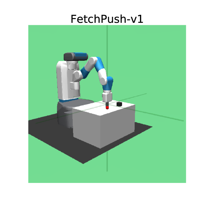
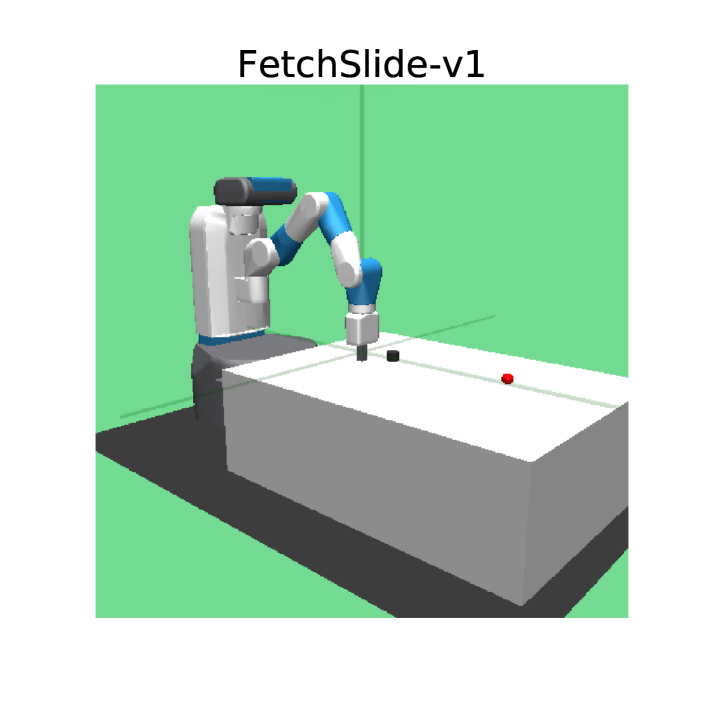
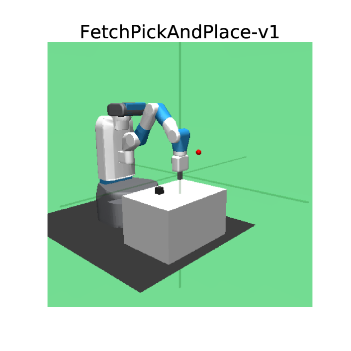
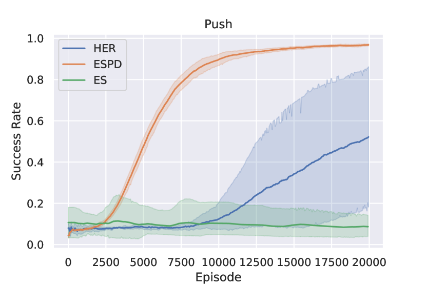
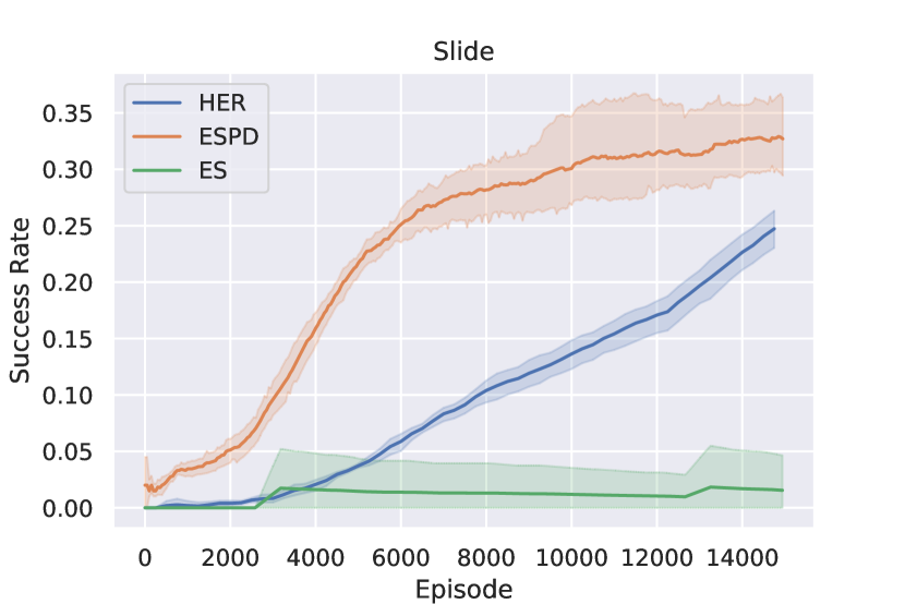
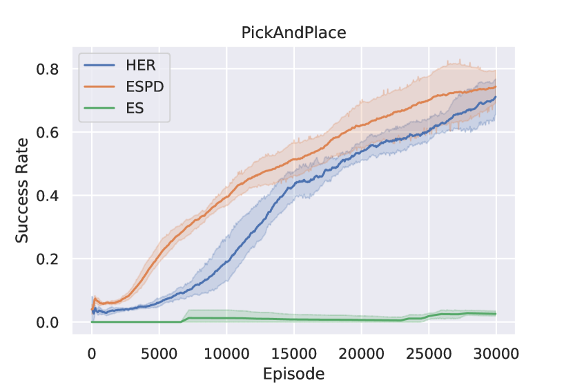
We demonstrate the proposed method on the Fetch Benchmarks. Specifically, we evaluate our method on the FetchPush, FetchSlide and FetchPickAndPlace environments, as shown in Fig.3. We compare our proposed method with the HER 3, 29 released in OpenAI Baselines 14 and the Evolution Strategy 33 which is a counterpart of our method with parameter noise. As PCHID 40 can be regarded as a special case of ESPD if we gradually increase the hyper-parameter Horizon in ESPD from to , the performance of PCHID is upper-bounded by ESPD and we do not include it as a baseline. Such result can be inferred from our ablation study on the Horizon in the next section, which shows smaller limits the performance, and achieves worse learning efficiency than , the default hyper-parameter used in ESPD222In FetchSlide, our ablation studies in the next section shows outperforms ..
Fig.4 shows the comparison of different approaches. For each environment, we conduct 5 experiments with different random seeds and plot the averaged learning curve. Our method shows superior learning efficiency and can learn to solve the task in fewer episodes in all the three environments.
4.2 Ablation Studies
Exploration Factor
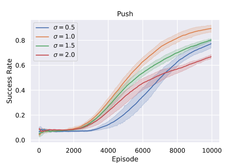
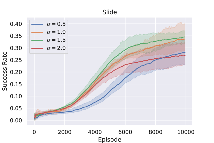
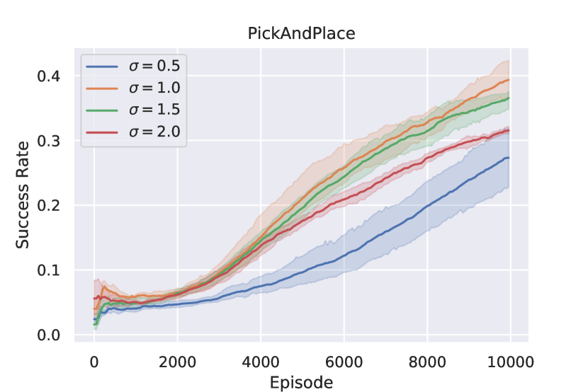
The exploration factor controls the randomness of behavior policy and therefore determines the behavior of generated samples. While larger helps the agents to benefit exploration by generating samples with large variance, smaller helps to generate a biased sample with little variance. Here we need to select a proper to balance the variance and bias. Fig.5 shows our ablation study on the selection of different exploration factors. The results are generated with 5 different random seeds. We find in all environments, the exploration factor provides sufficient exploration and relatively high learning efficiency.
Horizon
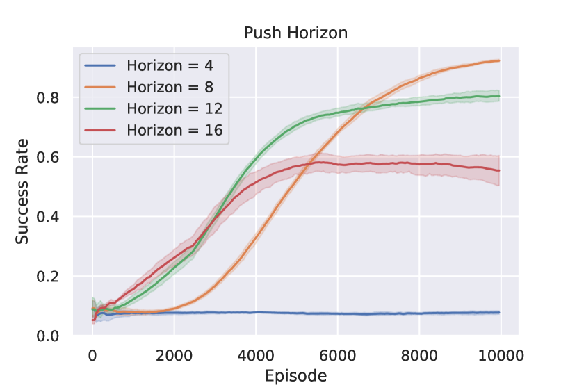
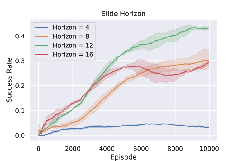
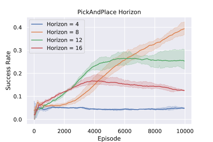
In our proposed method, the parameter of Horizon determines the maximal length of sample trajectories the policy can learn from. Intuitively, smaller decreases the learning efficiency as the policy is limited by its small horizon, making it hard to plan for the tasks that need more steps to solve. On the other hand, larger will provide a better concept of the local as well as global geometry of the state space, and thus the agent may learn to solve more challenging tasks. However, using large introduces more interactions with the environment, and needs more computation time. Moreover, as the tasks normally do not need lots of steps to finish, when the Horizon is getting too large, more noisy actions will be collected and be considered as better solutions and hence impede the learning performance. Fig.6 shows our ablation studies on the selection of Horizon . The results are generated with 5 different random seeds. We find that provides satisfying results in all of the three environments.
5 Related Work
Learning with Experts and Policy Distillation
Imitation Learning (IL) approaches introduce expert data in the learning of a agent 30, 31, while similar techniques are used in the literature of Learning from Demonstrations (LfD) 6, 34, 4, where experience of human expert will be collected to help the learning of an agent. Those methods are further extended in the setting of Deep Q-learning 24, 21, combined with DDPG 23, 25 or to learn from imperfect expert data 18.
Policy Distillation was proposed to extract the policy of a trained RL agent with a smaller network to improve the efficiency as well as the final performance or combine several task-specific agents together 32. Latter extensions proposed to improve the learning efficiency 37, enhance multi-task learning 43, 5.
All of those methods start from a trained expert agent or human expert experience that can solve a specific task 13. As a comparison, our proposed method focus on extracting knowledge from stochastic behaviors, which is capable to act as a feasible policy itself with regard to the primal task.
Evolution Strategies and Parameter Noise
The Evolution Strategy (ES) was proposed by Salimans et al. 33 as an alternative to standard RL approaches, where the prevailing temporal difference based value function updates or policy gradient methods are replaced as perturbations on the parameter space to resemble the evolution. Later on, Campos et al. 11 improved the efficiency of ES by means of importance sampling. Besides, the method was also extended to be combined with Novelty-Seeking to further improve the performance 12.
Thereafter, Plappert et al. 28 proposed to use Parameter Noise as an alternative to the action space noise injection for better exploration. They show such a perturbation on the parameter space can be not only used for ES methods, but also collected to improve the sample efficiency by combining it with traditional RL methods.
While previous ES algorithms apply perturbations on the parameter noise and keep the best-performed variates, our approach implicitly execute the policy evolution by distilling better behaviors, therefore our approach can be regarded as an Evolutiaon Strategy based on action space perturbation.
Supervised and Self-Imitate Approaches in RL
Recently, several works put forward to use supervised learning to improve the stability and efficiency of RL. Zhang et al. 45 propose to utilize supervised learning to tackle the overly large gradients problem in policy gradient methods. In order to improve sample efficiency, the work chose to first design a target distribution proposal and then used supervised learning to minimize the distance between present policy and the target policy distribution. The Upside-Down RL proposed by Schmidhuber 36 used supervised learning to mapping states and rewards into action distributions, and therefore acted as a normal policy in RL. Their experiments show that the proposed UDRL method outperforms several baseline methods 39. In the work of Sun et al. 40, a curriculum learning scheme is utilized to learn policies recursively. The self-imitation idea relevant to ESPD is also discussed in the concurrent work of Ghosh et al. 19, but ESPD further uses the SELECT function to improve the quality of collected data for self-imitation learning.
6 Conclusion
In this work we focus on developing a practical algorithm that can evolve to solve the GCRS problems by distilling knowledge from a series of its stochastic variants. The key insight behind our proposed method is based on our SDE formulation of the GCRS tasks: such tasks can be solved by learning to reduce the FHT. Our experiments on the OpenAI Fetch Benchmarks show that the proposed method, Evolutionary Stochastic Policy Distillation, has high learning efficiency as well as stability with regard to two baseline methods, the Evolution Strategies and Hindsight Experience Replay.
References
- Alili et al. [2005] Alili, L., Patie, P., and Pedersen, J. L. Representations of the first hitting time density of an ornstein-uhlenbeck process. Stochastic Models, 21(4):967–980, 2005.
- Kaelbling [1993] Kaelbling, Leslie Pack. Learning to achieve goals In the 13th International Joint Conferences on Artificial Intelligence, pp. 1094–1099. Citeseer, 1993.
- Andrychowicz et al. [2017] Andrychowicz, M., Wolski, F., Ray, A., Schneider, J., Fong, R., Welinder, P., McGrew, B., Tobin, J., Pieter Abbeel, O., and Zaremba, W. Hindsight experience replay. In Guyon, I., Luxburg, U. V., Bengio, S., Wallach, H., Fergus, R., Vishwanathan, S., and Garnett, R. (eds.), Advances in Neural Information Processing Systems 30, pp. 5048–5058. Curran Associates, Inc., 2017. URL http://papers.nips.cc/paper/7090-hindsight-experience-replay.pdf.
- Argall et al. [2009] Argall, B. D., Chernova, S., Veloso, M., and Browning, B. A survey of robot learning from demonstration. Robotics and autonomous systems, 57(5):469–483, 2009.
- Arora et al. [2018] Arora, H., Kumar, R., Krone, J., and Li, C. Multi-task learning for continuous control. arXiv preprint arXiv:1802.01034, 2018.
- Atkeson & Schaal [1997] Atkeson, C. G. and Schaal, S. Robot learning from demonstration. In ICML, volume 97, pp. 12–20. Citeseer, 1997.
- Barto & Mahadevan [2003] Barto, A. G. and Mahadevan, S. Recent advances in hierarchical reinforcement learning. Discrete event dynamic systems, 13(1-2):41–77, 2003.
- Bengio et al. [2009] Bengio, Y., Louradour, J., Collobert, R., and Weston, J. Curriculum learning. In Proceedings of the 26th annual international conference on machine learning, pp. 41–48, 2009.
- Bishop [1994] Bishop, C. M. Mixture density networks. 1994.
- Bracewell & Bracewell [1986] Bracewell, R. N. and Bracewell, R. N. The Fourier transform and its applications, volume 31999. McGraw-Hill New York, 1986.
- Campos et al. [2018] Campos, V., Giro-i Nieto, X., and Torres, J. Importance weighted evolution strategies. arXiv preprint arXiv:1811.04624, 2018.
- Conti et al. [2018] Conti, E., Madhavan, V., Such, F. P., Lehman, J., Stanley, K., and Clune, J. Improving exploration in evolution strategies for deep reinforcement learning via a population of novelty-seeking agents. In Advances in neural information processing systems, pp. 5027–5038, 2018.
- Czarnecki et al. [2019] Czarnecki, W. M., Pascanu, R., Osindero, S., Jayakumar, S. M., Swirszcz, G., and Jaderberg, M. Distilling policy distillation. arXiv preprint arXiv:1902.02186, 2019.
- Dhariwal et al. [2017] Dhariwal, P., Hesse, C., Klimov, O., Nichol, A., Plappert, M., Radford, A., Schulman, J., Sidor, S., Wu, Y., and Zhokhov, P. Openai baselines. https://github.com/openai/baselines, 2017.
- Dietterich [2000] Dietterich, T. G. Hierarchical reinforcement learning with the maxq value function decomposition. Journal of artificial intelligence research, 13:227–303, 2000.
- Fujimoto et al. [2018a] Fujimoto, S., Meger, D., and Precup, D. Off-policy deep reinforcement learning without exploration. arXiv preprint arXiv:1812.02900, 2018a.
- Fujimoto et al. [2018b] Fujimoto, S., Van Hoof, H., and Meger, D. Addressing function approximation error in actor-critic methods. arXiv preprint arXiv:1802.09477, 2018b.
- Gao et al. [2018] Gao, Y., Lin, J., Yu, F., Levine, S., Darrell, T., et al. Reinforcement learning from imperfect demonstrations. arXiv preprint arXiv:1802.05313, 2018.
- Ghosh et al. [2019] Ghosh, D., Gupta, A., Fu, J., Reddy, A., Devine, C., Eysenbach, B., and Levine, S. Learning to reach goals without reinforcement learning. arXiv preprint arXiv:1912.06088, 2019.
- Ha & Schmidhuber [2018] Ha, D. and Schmidhuber, J. World models. arXiv preprint arXiv:1803.10122, 2018.
- Hester et al. [2018] Hester, T., Vecerik, M., Pietquin, O., Lanctot, M., Schaul, T., Piot, B., Horgan, D., Quan, J., Sendonaris, A., Osband, I., et al. Deep q-learning from demonstrations. In Thirty-Second AAAI Conference on Artificial Intelligence, 2018.
- Kakutani [1944] Kakutani, S. 143. two-dimensional brownian motion and harmonic functions. Proceedings of the Imperial Academy, 20(10):706–714, 1944.
- Lillicrap et al. [2015] Lillicrap, T. P., Hunt, J. J., Pritzel, A., Heess, N., Erez, T., Tassa, Y., Silver, D., and Wierstra, D. Continuous control with deep reinforcement learning. arXiv preprint arXiv:1509.02971, 2015.
- Mnih et al. [2015] Mnih, V., Kavukcuoglu, K., Silver, D., Rusu, A. A., Veness, J., Bellemare, M. G., Graves, A., Riedmiller, M., Fidjeland, A. K., Ostrovski, G., et al. Human-level control through deep reinforcement learning. Nature, 518(7540):529–533, 2015.
- Nair et al. [2018] Nair, A., McGrew, B., Andrychowicz, M., Zaremba, W., and Abbeel, P. Overcoming exploration in reinforcement learning with demonstrations. In 2018 IEEE International Conference on Robotics and Automation (ICRA), pp. 6292–6299. IEEE, 2018.
- Ng et al. [1999] Ng, A. Y., Harada, D., and Russell, S. Policy invariance under reward transformations: Theory and application to reward shaping. In ICML, volume 99, pp. 278–287, 1999.
- Pachocki et al. [2018] Pachocki, J., Brockman, G., Raiman, J., Zhang, S., Pondé, H., Tang, J., Wolski, F., Dennison, C., Jozefowicz, R., Debiak, P., et al. Openai five, 2018. URL https://blog. openai. com/openai-five, 2018.
- Plappert et al. [2017] Plappert, M., Houthooft, R., Dhariwal, P., Sidor, S., Chen, R. Y., Chen, X., Asfour, T., Abbeel, P., and Andrychowicz, M. Parameter space noise for exploration. arXiv preprint arXiv:1706.01905, 2017.
- Plappert et al. [2018] Plappert, M., Andrychowicz, M., Ray, A., McGrew, B., Baker, B., Powell, G., Schneider, J., Tobin, J., Chociej, M., Welinder, P., et al. Multi-goal reinforcement learning: Challenging robotics environments and request for research. arXiv preprint arXiv:1802.09464, 2018.
- Pomerleau [1991] Pomerleau, D. A. Efficient training of artificial neural networks for autonomous navigation. Neural computation, 3(1):88–97, 1991.
- Ross et al. [2011] Ross, S., Gordon, G., and Bagnell, D. A reduction of imitation learning and structured prediction to no-regret online learning. In Proceedings of the fourteenth international conference on artificial intelligence and statistics, pp. 627–635, 2011.
- Rusu et al. [2015] Rusu, A. A., Colmenarejo, S. G., Gulcehre, C., Desjardins, G., Kirkpatrick, J., Pascanu, R., Mnih, V., Kavukcuoglu, K., and Hadsell, R. Policy distillation. arXiv preprint arXiv:1511.06295, 2015.
- Salimans et al. [2017] Salimans, T., Ho, J., Chen, X., Sidor, S., and Sutskever, I. Evolution strategies as a scalable alternative to reinforcement learning. arXiv preprint arXiv:1703.03864, 2017.
- Schaal [1997] Schaal, S. Learning from demonstration. In Advances in neural information processing systems, pp. 1040–1046, 1997.
- Schaul et al. [2015] Schaul, T., Horgan, D., Gregor, K., and Silver, D. Universal value function approximators. In Bach, F. and Blei, D. (eds.), Proceedings of the 32nd International Conference on Machine Learning, volume 37 of Proceedings of Machine Learning Research, pp. 1312–1320, Lille, France, 07–09 Jul 2015. PMLR. URL http://proceedings.mlr.press/v37/schaul15.html.
- Schmidhuber [2019] Schmidhuber, J. Reinforcement learning upside down: Don’t predict rewards–just map them to actions. arXiv preprint arXiv:1912.02875, 2019.
- Schmitt et al. [2018] Schmitt, S., Hudson, J. J., Zidek, A., Osindero, S., Doersch, C., Czarnecki, W. M., Leibo, J. Z., Kuttler, H., Zisserman, A., Simonyan, K., et al. Kickstarting deep reinforcement learning. arXiv preprint arXiv:1803.03835, 2018.
- Silver et al. [2016] Silver, D., Huang, A., Maddison, C. J., Guez, A., Sifre, L., Van Den Driessche, G., Schrittwieser, J., Antonoglou, I., Panneershelvam, V., Lanctot, M., et al. Mastering the game of go with deep neural networks and tree search. nature, 529(7587):484, 2016.
- Srivastava et al. [2019] Srivastava, R. K., Shyam, P., Mutz, F., Jaśkowski, W., and Schmidhuber, J. Training agents using upside-down reinforcement learning. arXiv preprint arXiv:1912.02877, 2019.
- Sun et al. [2019] Sun, H., Li, Z., Liu, X., Lin, D., and Zhou, B. Policy continuation with hindsight inverse dynamics. In Advances in Neural Information Processing Systems, pp. 10265–10275, 2019.
- Sutton et al. [1998] Sutton, R. S., Barto, A. G., et al. Introduction to reinforcement learning, volume 135. MIT press Cambridge, 1998.
- Tamar et al. [2016] Tamar, A., Wu, Y., Thomas, G., Levine, S., and Abbeel, P. Value iteration networks. In Advances in Neural Information Processing Systems, pp. 2154–2162, 2016.
- Teh et al. [2017] Teh, Y., Bapst, V., Czarnecki, W. M., Quan, J., Kirkpatrick, J., Hadsell, R., Heess, N., and Pascanu, R. Distral: Robust multitask reinforcement learning. In Advances in Neural Information Processing Systems, pp. 4496–4506, 2017.
- Vinyals et al. [2019] Vinyals, O., Babuschkin, I., Czarnecki, W. M., Mathieu, M., Dudzik, A., Chung, J., Choi, D. H., Powell, R., Ewalds, T., Georgiev, P., et al. Grandmaster level in starcraft ii using multi-agent reinforcement learning. Nature, 575(7782):350–354, 2019.
- Zhang et al. [2019] Zhang, C., Li, Y., and Li, J. Policy search by target distribution learning for continuous control. arXiv preprint arXiv:1905.11041, 2019.
Appendix A On the Selection of Exploration Factor
In Algorithm 1, the behavior policy is composed of the deterministic target policy , and an exploration term . During the learning process, provides a biased estimation of the feasible policy without variance, while the exploration term provides unbiased exploration with variance. The Eq.5 becomes
| (9) |
where is an unknown bias introduced by function approximation error or extrapolation error 16 due to the limited number of samples in Algorithm 1.
Intuitively, a large exploration factor, i.e.large , will lead to better exploration thus can help reduce the bias introduced by the , while smaller can reduce the variance, but expose the bias. This is exactly the dilemma of Exploration-Exploitation (E&E) 41. We further introduce an effective annealing method to adjust , the exploration factor to tackle the E&E challenge.
In the following section, we provide analysis and numerical experiment result based on the special case we have mentioned above to interpret how the exploration factor helps to correct the bias.
A.1 Revisit the Special Case: Navigation in the Euclidean Space
At the beginning of learning, the policy is initialized randomly. The only way to cross the target region at this moment is to utilize large exploration term, i.e.with large . As the learning continues with limited experience, bias might be introduced into Eq.6
| (10) |
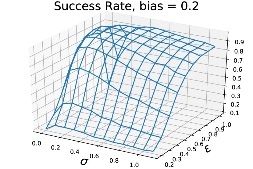
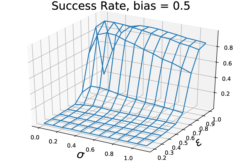
where denotes the bias. One the one hand, such bias may lead to extremely bad solutions if we do not keep a exploration term for bias correction 16. On the other hand, while the policy becomes more capable of navigating in the state space to reach the goal, large exploration term will hinder the agent to step into the goal region. Here we conduct a numerical simulation to show the dependencies of Success Rate, i.e.the proportion that successfully hit the goal region in a 2-D Euclidean space navigation task, on the value of .
A.2 Numerical Result
According to the previous analysis, the exploration with a random behaved policy in a GCRS task is like a random walk in the state space. Distinguished from the well known fact that a drunk man will find his way home, but a drunk bird may get lost forever 22, 10, in most cases, the systems we are concerned about have finite boundaries, and the goal, instead of a single point in the state space, always has a non-trivial radius. Therefore, in known dynamics, we can simulate the behavior of policy at different learning state, e.g., with different bias , goal-awareness , and investigate how the exploration factor affects the learning outcomes.
Our simulation is based on a bounded region of size , for each episode, a current state and goal are generated randomly in the region. At each timestep, the state updates according to Eq.10, with normalized step length. The success rate shows the probability of hitting the goal within a finite time horizon . In our simulation, we apply tabular fixed random bias with different scale (i.e., and ), and set , , maximal step length and goal radius .
The result is shown in Fig.7. Smaller bias enables success rate increases when the goal-awareness is small. As goal awareness increase, the performance of success rate relies on the selection of exploration factor. For small exploration factors, the performance of biased policy will drastically be hindered, while proper exploration factor value will fix such a problem. Such imperfectness, e.g., the bias is unavoidable when parameterizing the policy with a neural network, hence we maintain a small exploration factor even when evaluating a policy for bias correction. The detailed comparison with different exploration factor in both training and testing phase is discussed in the experiment section.
A.3 Evaluation Noise
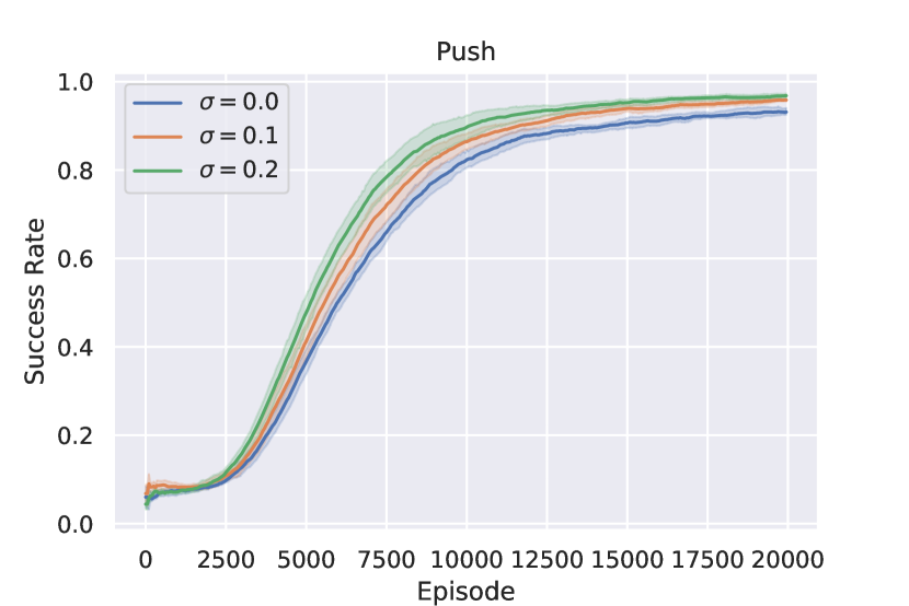
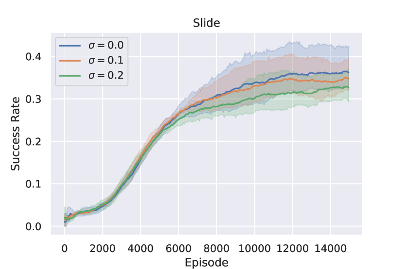
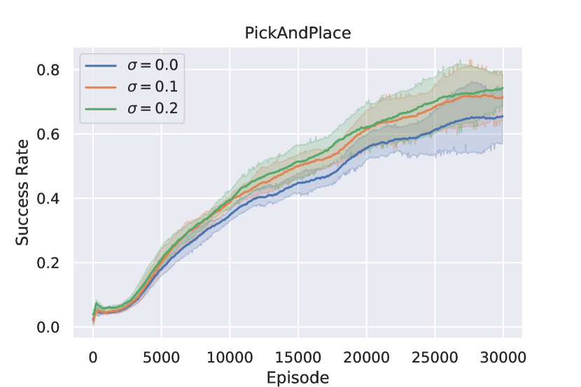
As we have shown in the numerical simulation, the bias of learned deterministic policy reduces the success rate. Such bias can be attributed to the extrapolation error 16. Consequently, we introduce a Gaussian noise term in the learned policy to form a stochastic policy for robustness. Our ablation studies on the selection of different scales of such noise terms are shown in Fig.8. The results are generated with 5 different random seeds, showing proper noise terms can help to overcome the extrapolation error and therefore improve the evaluation performance. It worths noting that applying larger noise in the game of FetchSlide will lead to performance decay, as the game relies on precise manipulation: after the robotic arm hitting the block, the block will become out of reach, and therefore the agent can not correct the error anymore.