High order numerical integrators for single integrand Stratonovich SDEs

Abstract

We show that applying any deterministic B-series method of order $p_{d}$ with a random step size to single integrand SDEs gives a numerical method converging in the mean-square and weak sense with order $\lfloor p_{d}/2\rfloor$. As an application, we derive high order energy-preserving methods for stochastic Poisson systems as well as further geometric numerical schemes for this wide class of Stratonovich SDEs.

1 Introduction

The last years have seen a great interest in the numerical analysis of single integrand Stratonovich stochastic differential equations

$$\,\mathrm{d}X(t)=f(X(t))\left(\lambda\,\mathrm{d}t+\sigma\circ\,\mathrm{d}W(t))=f(X(t)\right)\circ\,\mathrm{d}\mu(t),\qquad{X}(t_{0})=x_{0},$$ (1)

see, e. g. [3, 26, 25, 8, 27, 18, 24, 1, 9, 37, 11, 22, 23] as well as to the text below. Here, $t\geq t_{0}\geq 0$, $x_{0}\in\mathbb{R}^{d}$, $f\colon\mathbb{R}^{d}\to\mathbb{R}^{d}$, $(W(t))_{t\geq 0}$ is a standard one-dimensional Wiener process, $\lambda\in\{0,1\}$ and $\sigma\in\mathbb{R}$ are given constants, and $\mu({s}):=\lambda{s}+\sigma W(s)$ for $s\geq 0$.

Stochastic differential equations (SDEs) of this form arise, e. g., when the right-hand side of an ordinary differential equation (ODE) model is randomly perturbed. Interesting applications are:

Example 1 (Fatigue cracking [34]).

$$\,\mathrm{d}X(t)=aX^{p}(t)\,\mathrm{d}t+bX^{p}(t)\circ\,\mathrm{d}W(t),\qquad p>1,a,b\in\mathbb{R}.$$

Example 2 (Stochastic Hamiltonian systems [35, 25]).

$$\,\mathrm{d}X(t)=J^{-1}\nabla H(X(t))\left(\,\mathrm{d}t+c\circ\,\mathrm{d}W(t)\right),\qquad J=\begin{pmatrix}0&-I\\ I&0\end{pmatrix},c\in\mathbb{R}.$$

Example 3 (Stochastic perturbations of Poisson systems [9]).

$$\,\mathrm{d}X(t)=B(X(t))\nabla H(X(t))\left(\,\mathrm{d}t+c\circ\,\mathrm{d}W(t)\right),\qquad B=-B^{\top},c\in\mathbb{R}.$$

In the present communication, we generalize the main results from [11] from Runge–Kutta methods to B-series methods. In particular, this permits to show that when applying any (deterministic) B-series numerical integrators of order $p_{d}$ to (1) by replacing the deterministic step size $h$ in the numerical scheme by $\lambda h+\sigma(W(t+h)-W(t))$ when calculating one step of the approximation on the time interval $[t,t+h]$ respectively, one then automatically obtains a time integrator with step size $h$ of mean-square as well as weak order $\lfloor p_{d}/2\rfloor$ for the SDE (1). We recall that the notation $\lfloor x\rfloor$ denotes the floor function of a real number $x$.

On top of that, it can easily be observed that, in general, when a (deterministic) numerical integrator possesses some geometric properties, then the same geometric properties hold for the time integrator applied to single integrand SDEs (1). This observation thus allows to carry forward various results already obtained in the literature as well as new ones, see for instance Section 3 below.

B-series methods encompass any reasonable one-step time integrators for ODEs: Besides Runge–Kutta methods [16, 15], other one-step methods can be represented as B-series, e. g. Taylor methods [2, 13, 14], averaged vector field methods [29, 7], and $q$-derivative Runge–Kutta methods [16].

2 Convergence of B-series methods applied to single integrand SDEs

B-series for solutions to SDEs and their numerical solution by stochastic Runge–Kutta methods have been developed in [4, 5] to study strong convergence in the Stratonovich case, in [33, 32] for strong converge in the Itô as well as the Stratonovich case, in [21] and [20] to study weak convergence in the Stratonovich case and in [30, 31] to study weak convergence in both the Itô and the Stratonovich case. A uniform and self-contained theory for the construction of stochastic B-series for the exact solution of SDEs and its numerical approximation by stochastic Runge–Kutta methods is given in [12]. Based on the notation used there, in [11] the B-series for the exact solution and Runge–Kutta approximations of single-integrand SDEs were derived. For convenience, we summarize the results we will need in the following. Due to the single integrand we do, similar to the ODE case [6], only need non-colored trees in the expansion of the solution.

Definition 1 (Trees).

The set of rooted trees $T$ related to single-integrand SDEs is recursively defined as follows:

1. The empty tree $\emptyset$ and the graph $\bullet=[\emptyset]$ with only one vertex belong to $T$.

For a positive integer $\kappa$, let $\tau=[\tau_{1},\tau_{2},{\dots},\tau_{\kappa}]$ be the tree formed by joining the subtrees $\tau_{1},\tau_{2},{\dots},\tau_{\kappa}$ each by a single branch to a common root.

1. If $\tau_{1},\tau_{2},{\dots},\tau_{\kappa}\in T$ then $\tau=[\tau_{1},\tau_{2},{\dots},\tau_{\kappa}]\in T$.

Definition 2 (Elementary differentials).

For a tree $\tau\in T$ the elementary differential is a mapping $F(\tau):\mathbb{R}^{d}\rightarrow\mathbb{R}^{d}$ defined recursively by

1. $F(\emptyset)({x})={x}$,
   

2. $F(\bullet)({x})=f({x})$,
   

3. If $\tau=[\tau_{1},\tau_{2},{\dots},\tau_{\kappa}]\in T\setminus\{\emptyset\}$ then

   $$F(\tau)({x})=f^{(\kappa)}({x})\big{(}F(\tau_{1})({x}),F(\tau_{2})({x}),{\dots},F(\tau_{\kappa})({x})\big{)}$$

where ${x}\in\mathbb{R}^{d}$.

Definition 3 (B-series).

Consider for each $\tau\in T$ a stochastic process $(\phi(\tau)(h))_{h\geq 0}$ satisfying

$$\phi(\emptyset)\equiv 1\;\text{ and }\;\phi(\tau)(0)=0,\quad\text{for }\tau\in T\backslash\{\emptyset\}.$$

Let ${x}\in\mathbb{R}^{d}$ and $h\in\mathbb{R}$. A (stochastic) B-series is then a formal series of the form

$$B(\phi,{x};h)=\sum_{\tau\in T}\alpha(\tau)\cdot\phi(\tau)(h)\cdot F(\tau)({x}),$$

where $\alpha:T\rightarrow\mathbb{Q}$ is given by

$$\alpha(\emptyset) =1, \alpha(\bullet) =1, \alpha(\tau=[\tau_{1},\cdots,\tau_{\kappa}]) =\frac{1}{r_{1}!r_{2}!\cdots r_{q}!}\prod_{j=1}^{\kappa}\alpha(\tau_{j}),$$

where $r_{1},r_{2},{\dots},r_{q}$ count equal trees among $\tau_{1},\tau_{2},{\dots},\tau_{\kappa}$.

We are now able to state the B-series of the exact solution to the SDE (1), see also [12, 33]. In the following, $\rho(\tau)$ denotes the number of nodes in a tree $\tau$.

Theorem 1 ([11]).

Let $\gamma:T\rightarrow\mathbb{N}$ be given by

$$\gamma(\emptyset)=1,\qquad\gamma(\bullet)=1,$$

$$\gamma([\tau_{1},\dots,\tau_{\kappa}])=\rho([\tau_{1},\dots,\tau_{\kappa}])\prod_{j=1}^{\kappa}\gamma(\tau_{j}).$$

Then the solution $X({t+}h)$ of (1) starting at the point $(t,{x})$ can be written as a B-series $B({\varphi_{{t}}},{x};h)$ with

$${\varphi_{{t}}}(\tau)(h)=\frac{{\mu_{{t}}}(h)^{\rho(\tau)}}{\gamma(\tau)}\qquad\text{ for }\tau\in T$$ (2)

where

$${\mu_{{t}}}(s):=\mu(t+s)-\mu(t)=\lambda s+\sigma(W(t+{s}){-W(t)}).$$ (3)

That is, the B-series of the exact solution of (1) coincides with the one of the exact solution of an ODE (i. e. when $\lambda=1$, $\sigma=0$) when replacing ${\mu_{{t}}}(h)$ with $h$.

Next, we derive the B-series for the numerical solution of the single integrand SDE (1). To do this, we consider B-series methods for the ODE $\,\mathrm{d}X(t)=f(X(t))\,\mathrm{d}t$. Such methods can be written as [15]

$$Y(t+h)=B({\Phi_{{t}}},x;h)$$ (4)

with ${{\Phi_{{t}}}}(\tau)(h)=h^{\rho(\tau)}\cdot\hat{\Phi}(\tau)$ where $\hat{\Phi}:T\to\mathbb{R}$ fulfilling $\hat{\Phi}(\emptyset)=1$. Replacing $h$ by ${\Delta_{{t,t+h}}\mu}={\mu_{{t}}}(h)$ defined in (3) we consider therefore the following B-series method for solving (1):

Definition 4.

Given an ODE-B-series method (4) for the ODE $\,\mathrm{d}X(t)=f(X(t))\,\mathrm{d}t$, the corresponding ODE-B-series method for (1) is given by

$$Y(t+h)=B({\Phi^{\mu}_{{t}}},x;h),$$ (5)

where ${\Phi^{\mu}_{{t}}}(\tau){(h)}={(}{\Delta_{{{t,t+h}}}\mu}{)}^{\rho(\tau)}\hat{\Phi}(\tau)$.

Now we give the definitions of both weak and strong convergence used in this note.

Let $C_{P}^{l}(\mathbb{R}^{d},\mathbb{R}^{\hat{d}})$ denote the space of all $g\in C^{l}(\mathbb{R}^{d},\mathbb{R}^{\hat{d}})$ fulfilling a polynomial growth condition [19] and $I^{{\tilde{h}}}$ be the discretized time interval on which the numerical approximations are calculated.

Definition 5.

A time discrete approximation $Y=(Y(t))_{t\in{I^{{\tilde{h}}}}}$ converges weakly with order $p$ to $X$ at time $t\in{I^{{\tilde{h}}}}$ as the maximum step size ${\tilde{h}}\rightarrow 0$ if for each $g\in C_{P}^{2(p+1)}(\mathbb{R}^{d},\mathbb{R})$ there exist a constant $C_{g}$ and a finite $\delta_{0}>0$ such that

$$|\operatorname{E}(g(Y(t)))-\operatorname{E}(g(X(t)))|\leq C_{g}\,{\tilde{h}}^{p}$$

holds for each ${\tilde{h}}\in\,]0,\delta_{0}[\,$.

Whereas weak approximation methods are used to estimate the expectation of functionals of the solution, strong approximation methods approach the solution path-wise. In this article, next to weak convergence, we will consider mean-square instead of strong convergence.

Definition 6.

A time discrete approximation $Y=(Y(t))_{t\in{I^{{\tilde{h}}}}}$ converges in the mean-square sense with order $p$ to $X$ at time $t\in{I^{{\tilde{h}}}}$ as the maximum step size ${\tilde{h}}\rightarrow 0$ if there exist a constant $C$ and a finite $\delta_{0}>0$ such that

$$\sqrt{\operatorname{E}(\|Y(t)-X(t)\|^{2})}\leq C\,{\tilde{h}}^{p}$$

holds for each ${\tilde{h}}\in\,]0,\delta_{0}[\,$.

Observe that, by Jensen’s inequality, mean-square convergence implies strong convergence of the same order.

We are now in position to state the main result of the present publication.

Theorem 2.

Assume that the B-series method (5) is of deterministic order $p_{d}$ and let $p_{\mu}=\lfloor p_{d}/2\rfloor$. Further, let $f\in C^{2p_{\mu}+1}(\mathbb{R}^{d},\mathbb{R}^{d})$ and $f$ and $f^{\prime}f$ fulfill a Lipschitz condition. Finally, assume

• for mean-square convergence, that all elementary differentials $F(\tau)$ fulfill a linear growth condition,

• respectively for weak convergence, that $f\in C_{P}^{2p_{\mu}+1}(\mathbb{R}^{d},\mathbb{R}^{d})$.

Then this very same B-series method is of mean-square as well as weak order $p_{\mu}$ when applied to the single integrand SDE (1) with step size ${\Delta_{{t,t+h}}\mu}$. For weak convergence, it suffices that ${\Delta_{{t,t+h}}\mu}$ is chosen such that at least the first $2p_{\mu}+1$ moments coincide with those of ${\mu_{{t}}}(h)$, and all the others are in $\mathcal{O}(h^{p_{\mu}+1})$.

Proof.

To prove this result, one first observes that the corresponding Theorem for Runge–Kutta methods [11, Theorem 1.1] only uses that the B-series of the exact and numerical solutions fulfil the properties summarized in Definition 4. One can then directly extend the proof to the present situation of B-series methods. ∎

3 Applications to geometric numerical integration of single integrand SDEs

Geometric properties of numerical schemes for single integrand SDEs (1) are closely related to those of numerical schemes for their corresponding ODEs. This relation, which holds for B-series as well as non B-series (e. g. volume preserving) methods, can be specified furthermore: In principle, when applying any deterministic geometric numerical integrators to single integrand SDEs (1) with random step size ${\Delta_{{t,t+h}}\mu}$, one then obtains the same geometric property as by the corresponding deterministic numerical scheme. This is because the random perturbation in some sense respects the geometric structure of the phase space. Hence, proofs of conservation properties in the deterministic setting can be adapted to single integrand Stratonovich SDEs (1). With the main idea used in this paper, one easily derives several results already obtained in the literature as well as new ones for geometric numerical integrators of single integrand SDEs (1):

1. If the deterministic numerical method preserves linear or quadratic invariants, so does it for single integrand SDEs. See the example below and e.g.  [17].

2. If the deterministic scheme is energy or invariant-preserving, then it is also energy or invariant-preserving for single integrand SDEs. See the example below and e.g.  [26, 9, 22, 23].

3. If the deterministic numerical method is symmetric, then it is also symmetric for the SDE (1).

4. If the deterministic time integrator is symplectic and $f(x)=J^{-1}\nabla H(x)$, then it is symplectic for single integrand SDEs, e.g.  [27, 25, 35].

5. Deterministic (symmetric) projection methods can be directly applied to single integrand SDEs with constraints, e.g.  [36].

6. If the deterministic numerical method is volume preserving, then it is also volume preserving for single integrand SDEs.

7. If the deterministic numerical scheme is a Poisson integrator and $f(x)=B(x)\nabla H(x)$, where $B(x)$ represents a Poisson bracket, then it is also a Poisson integrator for single integrand SDEs.

4 Application to stochastic perturbations of Poisson systems

As application of Theorem 2 and the principles of the previous section, we propose a high order energy-preserving and Casimir-preserving scheme for the stochastic rigid body [9]. The equations of motion of this stochastic rigid body are a Lie-Poisson system:

$$\begin{pmatrix}\,\mathrm{d}X_{[1]}\\ \,\mathrm{d}X_{[2]}\\ \,\mathrm{d}X_{[3]}\end{pmatrix}=\begin{pmatrix}0&-X_{[3]}&X_{[2]}\\ X_{[3]}&0&-X_{[1]}\\ -X_{[2]}&X_{[1]}&0\end{pmatrix}\begin{pmatrix}X_{[1]}/I_{1}\\ X_{[2]}/I_{2}\\ X_{[3]}/I_{3}\end{pmatrix}\bigl{(}\,\mathrm{d}t+c\circ\,\mathrm{d}W\bigr{)},$$ (6)

with some initial value $X(0)\in\mathbb{R}^{3}$ at $t_{0}=0$, where $X=(X_{[1]},X_{[2]},X_{[3]})^{\top}$ and $I=(I_{1},I_{2},I_{3})$ are the moments of inertia. The Hamiltonian

$$H(X)=\frac{1}{2}\big{(}X_{[1]}^{2}/I_{1}+X_{[2]}^{2}/I_{2}+X_{[3]}^{2}/I_{3}\big{)}$$

is thus a conserved quantity as well as the quadratic Casimir

$$C(X)=\|X\|_{2}^{2}=X_{[1]}^{2}+X_{[2]}^{2}+X_{[3]}^{2}.$$

Note that the right hand side $f$ of (6) is not globally Lipschitz continuous and does thus a priori not fulfill the conditions of Theorem 2. However, for methods that conserve the Casimir, we can replace $f$ by a function being zero outside a suitable ball and fulfilling the conditions of Theorem 2, e. g. replacing $f$ by

$$\tilde{f}(X)=f(X)\frac{\varphi(4C(X(0))-C(X))}{\varphi(C(X)-2C(X(0)))+\varphi(4C(X(0))-C(X))}$$

where

$$\varphi(r)=\begin{cases}0&\text{for }{r\leq 0}\\ e^{-1/r}&\text{for }r>0.\end{cases}$$

Note that $\tilde{f}(X)=f(X)$ for all $\|X\|_{2}\leq\sqrt{2}\|X(0)\|$ and $\tilde{f}(X)=0$ for all $\|X\|_{2}\geq 2\|X(0)\|$ (see e. g. [28]), and all derivatives of $\tilde{f}$ remain bounded. A similar modification can be made for numerical methods that preserve the Hamiltonian of the deterministic rigid body.
As a starting deterministic method, we choose the linear energy-preserving integrators of orders $2,4$ and $6$ from [10]. By Theorem 2, we thus expect a first, resp. second, resp. third strong and weak order energy-preserving numerical integrator for the stochastic rigid body (6), denoted by EPs1, EPs2, EPs3. Recall that these novel numerical methods are simply given by replacing the step size $h$ by $\lambda h+\sigma\Delta W_{n}$ in the deterministic scheme. 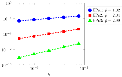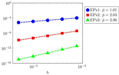The orders of convergence can be seen in Figures 1 and 2, where the numerically determined orders of convergence $\hat{p}$ correspond to the slopes of the dashed regression lines. The parameters for these numerical experiments are: $T_{end}=0.5,c=0.5,I=(0.345,0.653,1),X(0)=(0.8,0.6,0)$, and $200$ samples are used to approximate the expectations. We have checked that $200$ samples are sufficient for these numerical experiments. The reference solution is calculated with $h_{ref}=2^{-14}$ and EPs3.

Figure 1: Mean-square orders of convergence of the numerical schemes EPs1 to EPs3 for the stochastic rigid body (6). Used step sizes: $h=2^{-7}$ to $h=2^{-11}$.

Figure 2: Weak orders of convergence of the numerical schemes EPs1 to EPs3 for the second moments of approximations of solutions to the stochastic rigid body (6). Used step sizes: $h=2^{-7}$ to $h=2^{-11}$.

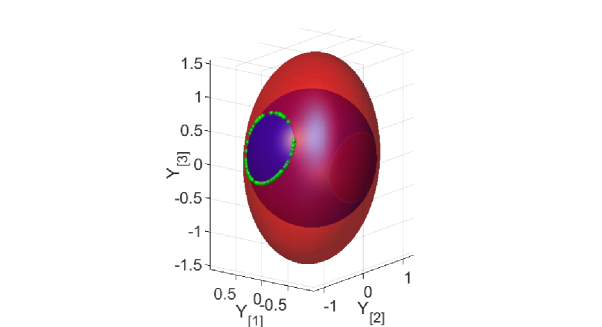
Furthermore, as it can be seen in Figure 3, for the example of the third order method, these numerical schemes not only preserve the energy but also the quadratic Casimir $C(X)$. This follows from the discussion in Section 3, as the numerical integrators from [10] are known to preserve quadratic Casimirs.

Figure 3: Numerical simulation with the third order method (one path) for the stochastic rigid body problem (green points) and the two invariants $H(Y)=H(Y(0))$ (blue) and $C(Y)=C(Y(0))$ (red), with $T_{end}=5$, $h=2^{-4}$, other parameters as before.

References

- [1] C. A. Anton, Y. S. Wong, and J. Deng. Symplectic schemes for stochastic Hamiltonian systems preserving Hamiltonian functions. Int. J. Numer. Anal. Model., 11(3):427–451, 2014.
- [2] R. Barrio. Performance of the Taylor series method for ODEs/DAEs. Appl. Math. Comput., 163(2):525–545, 2005.
- [3] J.-M. Bismut. Mécanique aléatoire, volume 866 of Lecture Notes in Mathematics. Springer-Verlag, Berlin-New York, 1981. With an English summary.
- [4] K. Burrage and P. M. Burrage. High strong order explicit Runge–Kutta methods for stochastic ordinary differential equations. Appl. Numer. Math., 22(1-3):81–101, 1996. Special issue celebrating the centenary of Runge-Kutta methods.
- [5] K. Burrage and P. M. Burrage. Order conditions of stochastic Runge-Kutta methods by -series. SIAM J. Numer. Anal., 38(5):1626–1646, 2000.
- [6] J. C. Butcher. Numerical methods for ordinary differential equations. 2nd revised ed. Hoboken, NJ: John Wiley & Sons. xix, 463 p., 2008.
- [7] E. Celledoni, R. I. McLachlan, D. I. McLaren, B. Owren, G. R. W. Quispel, and W. M. Wright. Energy-preserving Runge-Kutta methods. M2AN Math. Model. Numer. Anal., 43(4):645–649, 2009.
- [8] C. Chen, D. Cohen, and J. Hong. Conservative methods for stochastic differential equations with a conserved quantity. Int. J. Numer. Anal. Model., 13(3):435–456, 2016.
- [9] D. Cohen and G. Dujardin. Energy-preserving integrators for stochastic Poisson systems. Commun. Math. Sci., 12(8):1523–1539, 2014.
- [10] D. Cohen and E. Hairer. Linear energy-preserving integrators for Poisson systems. BIT, 51(1):91–101, 2011.
- [11] K. Debrabant and A. Kvæ rnø. Cheap arbitrary high order methods for single integrand SDEs. BIT, 57(1):153–168, 2017.
- [12] K. Debrabant and A. Kværnø. B-series analysis of stochastic Runge-Kutta methods that use an iterative scheme to compute their internal stage values. SIAM J. Numer. Anal., 47(1):181–203, 2008/09.
- [13] K. Debrabant and A. Kværnø. B-series analysis of iterated Taylor methods. BIT, 51(3):529–553, 2011.
- [14] K. Debrabant and A. Kværnø. Composition of stochastic B-series with applications to implicit Taylor methods. Appl. Numer. Math., 61(4):501–511, 2011.
- [15] E. Hairer, C. Lubich, and G. Wanner. Geometric numerical integration, volume 31 of Springer Series in Computational Mathematics. Springer-Verlag, Berlin, second edition, 2006. Structure-preserving algorithms for ordinary differential equations.
- [16] E. Hairer, S. P. Nørsett, and G. Wanner. Solving ordinary differential equations. I: Nonstiff problems. 2nd revised ed., 3rd corrected printing. Springer Series in Computational Mathematics 8. Berlin: Springer. xv, 528 p., 2010.
- [17] J. Hong, D. Xu, and P. Wang. Preservation of quadratic invariants of stochastic differential equations via Runge-Kutta methods. Appl. Numer. Math., 87:38–52, 2015.
- [18] J. Hong, S. Zhai, and J. Zhang. Discrete gradient approach to stochastic differential equations with a conserved quantity. SIAM J. Numer. Anal., 49(5):2017–2038, 2011.
- [19] P. E. Kloeden and E. Platen. Numerical solution of stochastic differential equations, volume 21 of Applications of Mathematics. Springer-Verlag, Berlin, 2 edition, 1999.
- [20] Y. Komori. Multi-colored rooted tree analysis of the weak order conditions of a stochastic Runge-Kutta family. Appl. Numer. Math., 57(2):147–165, 2007.
- [21] Y. Komori, T. Mitsui, and H. Sugiura. Rooted tree analysis of the order conditions of ROW-type scheme for stochastic differential equations. BIT, 37(1):43–66, 1997.
- [22] X. Li, Q. Ma, and X. Ding. High-order energy-preserving methods for stochastic Poisson systems. East Asian J. Appl. Math., 9(3):465–484, 2019.
- [23] X. Li, C. Zhang, Q. Ma, and X. Ding. Arbitrary high-order EQUIP methods for stochastic canonical Hamiltonian systems. Taiwanese J. Math., 23(3):703–725, 2019.
- [24] Q. Ma, D. Ding, and X. Ding. Symplectic conditions and stochastic generating functions of stochastic Runge-Kutta methods for stochastic Hamiltonian systems with multiplicative noise. Appl. Math. Comput., 219(2):635–643, 2012.
- [25] G. N. Milstein, Y. M. Repin, and M. V. Tretyakov. Numerical methods for stochastic systems preserving symplectic structure. SIAM J. Numer. Anal., 40(4):1583–1604, 2002.
- [26] T. Misawa. Energy conservative stochastic difference scheme for stochastic Hamilton dynamical systems. Japan J. Indust. Appl. Math., 17(1):119–128, 2000.
- [27] T. Misawa. Symplectic integrators to stochastic Hamiltonian dynamical systems derived from composition methods. Math. Probl. Eng., pages Art. ID 384937, 12, 2010.
- [28] J. Nestruev. Smooth manifolds and observables, volume 220 of Graduate Texts in Mathematics. Springer-Verlag, New York, 2003.
- [29] G. R. W. Quispel and D. I. McLaren. A new class of energy-preserving numerical integration methods. J. Phys. A, 41(4):045206, 7, 2008.
- [30] A. Rößler. Stochastic Taylor expansions for the expectation of functionals of diffusion processes. Stoch. Anal. Appl., 22(6):1553–1576, 2004.
- [31] A. Rößler. Rooted tree analysis for order conditions of stochastic Runge–Kutta methods for the weak approximation of stochastic differential equations. Stoch. Anal. Appl., 24(1):97–134, 2006.
- [32] A. Rößler. Runge-Kutta methods for the strong approximation of solutions of stochastic differential equations. SIAM J. Numer. Anal., 48(3):922–952, 2010.
- [33] A. Rößler. Stochastic Taylor expansions for functionals of diffusion processes. Stoch. Anal. Appl., 28(3):415–429, 2010.
- [34] K. Sobczyk. Stochastic models for fatigue damage of materials. Adv. in Appl. Probab., 19(3):652–673, 1987.
- [35] P. Wang, J. Hong, and D. Xu. Construction of symplectic Runge-Kutta methods for stochastic Hamiltonian systems. Commun. Comput. Phys., 21(1):237–270, 2017.
- [36] Z. Wang, C. Wang, Q. Ma, and X. Ding. Numerical simulations for stochastic differential equations on manifolds by stochastic symmetric projection method. Physica A: Statistical Mechanics and its Applications, page 123305, 2019.
- [37] A. Xiao and X. Tang. High strong order stochastic Runge-Kutta methods for Stratonovich stochastic differential equations with scalar noise. Numer. Algorithms, 72(2):259–296, 2016.