SFTM: Fast Comparison of Web Documents using Similarity-based Flexible Tree Matching

Abstract.

Tree matching techniques have been investigated in many fields, including web data mining and extraction, as a key component to analyze the content of web documents, existing tree matching approaches, like Tree-Edit Distance (TED) or Flexible Tree Matching (FTM), fail to scale beyond a few hundreds of nodes, which is far below the average complexity of existing web online documents and applications.

In this paper, we therefore propose a novel Similarity-based Flexible Tree Matching algorithm (SFTM), which is the first algorithm to enable tree matching on real-life web documents with practical computation times. In particular, we approach tree matching as an optimisation problem and we leverage node labels and local topology similarity in order to avoid any combinatorial explosion. Our practical evaluation demonstrates that our approach compares to the reference implementation of TED qualitatively, while improving the computation times by two orders of magnitude.

1. Introduction

The success of Internet has lead to the publication and the delivery of a deluge of web documents. In particular, web services and applications are heavily using XML and JSON standards to transfer information across the network as structured web documents. Inevitably, the success of these technologies has led to the definition of more complex and large web documents that keep evolving over time. However, keeping track of such changes remains a critical issue for the ecosystem and the research community. Examples of usages that require to detect or track changes in web documents include Web extraction (Reis et al., 2004; Yao et al., 2013; Zhai and Liu, 2005), Web testing (Stocco et al., 2017; Choudhary et al., 2011), comparison of Web service versions (Fokaefs et al., 2011), Web schema matching (Hao and Zhang, 2007) and automatic re-organization of websites (Kumar et al., 2011a).

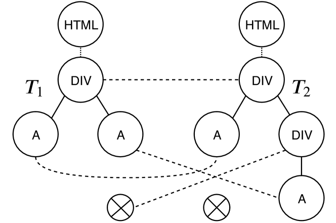
Figure 1. Example of a tree matching. Crossed circles are auxiliary no-match nodes enabling insertions and removals between trees.

As all of these usages share the need to compare Document Object Model (DOM) trees across multiples versions of a web document, several algorithms have been proposed to achieve this goal. The traditional approach, which is general to any kind of tree, is Tree Edit Distance (TED) (Tai, 1979) and can be computed in minimum $O(N^{3})$ time (Bringmann et al., 2018). Figure 1 illustrates the tree-matching problem. TED is a restriction of tree matching where descendants of matched nodes can only match with each others (ancestry restriction) and siblings order must be preserved. We executed a robust implementation of TED, named APTED (Pawlik and Augsten, 2015, 2016), on two instances of the DOM of YouTube, which took more than 4 minutes to propose a matching. Unfortunately, when processing and comparing a large dataset of Web documents, one cannot afford such computation times, which makes TED difficult to use in production.

The qualitative restrictions and speed limitations of TED therefore led to the development of alternative algorithms. (Fokaefs et al., 2011) extended TED with some additional move operations executed a posteriori to address the ancestry restriction. (Kumar et al., 2011b; Kumar et al., 2011a) developed her own Flexible Tree Matching (FTM) algorithm to address the ancestry restriction problem, while (Reis et al., 2004) developed a fast matching system based on top-down matching to extract news faster than TED does.

In the line of the aforementioned work, this paper aims at enabling the fast and non-restricted comparison of complex web documents. We propose an extended version of FTM, named Similarity-based Flexible Tree Matching (SFTM), that leverages similarity metrics to speed up the comparison. SFTM retains the advantage of FTM to offer a non-restricted tree matching while offering computation times much lower than even restricted versions of the problem. The algorithm exposes performance parameters to trade computation time and matching accuracy. To the best of our knowledge, SFTM is the first solution to match real-life web documents in practical time (e.g. SFTM matches the DOM of Youtube in less than a second compared to 4 minutes for APTED). Through empirical evaluation on real websites, we show that—for selected parameters—our implementation of SFTM qualitatively compares to APTED and empirically seems to scale in $O(n\cdot log(n))$ with the size of the considered DOM, thus making it applicable in many production contexts.

The remainder of this paper is organized as follows. Section 2 covers the related work. Section 3 introduces the Flexible Tree Matching (FTM) original algorithm. Section 4 presents Similarity-based Flexible Tree Matching (SFTM), our extension of FTM that leverages the node labels and local topology similarity to guide the comparison. Section 5 thoroughly evaluates our solution against the state of the art on a realistic dataset of web documents. Section 6 discusses the threats to validity of our contribution. Section 7 concludes and overviews some perspectives for this work.

2. Related Work

Tree Edit Distance (TED)

Comparing two trees is a problem that has been at the center of a significant amount of research. In 1979, Tai (Tai, 1979) introduced the Tree Edit Distance (TED) as a generalization of the standard edit distance problem applied to strings. Given two ordered labeled trees $T_{1}$ and $T_{2}$, the TED is defined as the minimal amount of node insertion, removal or relabel to transform $T_{1}$ into $T_{2}$, while different cost coefficients can be assigned to each type of operation. By following an optimal sequence of operations applied to $T_{1}$, it is possible to match the nodes between $T_{1}$ and $T_{2}$. This problem has been extensively studied since then to reduce the space and time complexity of the algorithm that computes the TED. To the best of our knowledge, the reference implementation available today is the All-Path Tree Edit Distance (APTED) (Pawlik and Augsten, 2011, 2015, 2016) with a complexity of $O(n^{2})$ in space and $O(n^{3})$ in time in the worst case, where $n$ is the total number of nodes ($n=|T_{1}|+|T_{2}|$). In our work, we consider APTED as the baseline to evaluate our contribution.

(Bringmann et al., 2018) showed that TED cannot be computed in worst case complexity lower than $O(n^{3})$. In order to circumvent this limitation, several restricted versions of the TED problem have been formulated. The Constrained Edit Distance (Zhang, 1995, 1996) is an edit distance where disjoint subtrees can only be mapped to disjoint subtrees. The Tree Alignment Distance (Jiang et al., 1994) is a TED where all insertions must be performed before any deletion. The Top-Down distance (Selkow, 1977) is computable in $O(|T_{1}||T_{2}|)$, but imposes as a restriction that the parents of nodes in a mapping must be in the mapping. The Bottom-Up distance (Valiente, 2001) between trees allows to build a mapping in linear time, but such mapping must respect the following constraint: if two nodes have been mapped, their respective children must also be part of the mapping. (Reis et al., 2004) proposes a variation of the Top-Down mapping, called Restricted Top-Down Mapping (RTDM), where replacement operations are restricted to the leaves of the trees, which delivers considerable speed gains, despite a theoretical worst case time complexity still in $O(N^{2})$. By definition TED already sets strong restrictions on produced matchings: sibling order and ancestry relationships must be preserved (Zhang, 1995). These restrictions are particularly problematic when matching two full web documents together (Kumar et al., 2011a). While above solutions improve computation times, they answer a restricted version of the TED problem leading to an even more restricted set of possible matchings.

Flexible Tree Matching (FTM)

In (Kumar et al., 2011a), TED is found to be unpractical when applied on DOM, as the resulting matching enforces ancestry relationship—i.e., once $n\in T_{1}$ and $m\in T_{2}$ have been matched, the descendants of $n$ can only be matched with the descendants of $m$, and vice versa. Consequently, Kumar et al. introduced the notion of Flexible Tree Matching (FTM), which relaxes the ancestry relationship constraint at the price of a strong complexity. It restricts its use to small HTML trees composed of hundreds of nodes, thus making it unpractical for modern web documents, often including thousands of nodes.

We therefore aim at reducing the complexity of the FTM algorithm in order to scale on complex web documents without enforcing restrictions on produced tree-matching solutions. More specifically, our contributions read as follows:

1. We develop an extended FTM algorithm, coined as Similarity-based Flexible Tree Matching (SFTM), by leveraging the notion of label similarity, and similarity propagation to reduce the computation time,

2. We apply mutations on real-life web documents, and provide a thorough evaluation of our implementation of SFTM, showing it outperforms state-of-the-art approaches in terms of scalability and performance, yet offering similar qualitative results.

3. Flexible Tree Matching

The Similarity-based Flexible Tree Matching (SFTM) we introduce in this paper is an extension of the Flexible Tree Matching Algorithm (FTM). This section therefore introduces the FTM algorithm, as originally proposed by Kumar et al. (Kumar et al., 2011a). We first describe the notations used throughout the rest of the paper, and then describe the main steps of the algorithm.

Building on the terminology from (Kumar et al., 2011b), we consider a matching between two labeled trees $T_{1}$ and $T_{2}$ comprising $|T_{1}|$ and $|T_{2}|$ nodes, respectively. We note $N=max(|T_{1}|,|T_{2}|)$.

Let us consider the complete bipartite graph $G$ between $T_{1}^{*}=T_{1}\cup{\Theta_{1}}$ and $T_{2}^{*}=T_{2}\cup{\Theta_{2}}$, where $\Theta_{1}$ and $\Theta_{2}$ are no-match nodes. The fact that $G$ is complete means that every nodes of $T_{1}^{*}$ shares exactly one edge with every nodes of $T_{2}^{*}$. An edge $e(n,m)\in E(G)$ between $n\in T_{1}^{*}$ and $m\in T_{2}^{*}$ represents the matching of $n$ with $m$. So, intuitively, $G$ represents all possible matchings between $T_{1}^{*}$ and $T_{2}^{*}$ (cf. Figure 2). We call matching and note $M\subset E(G)$, a subset of edges selected from $G$. A matching $M$ is said to be full iff each node in $T_{1}$ has exactly one edge in $M$ that links it to a node in $T_{2}^{*}$ and, inversely, each node in $T_{2}$ has exactly one edge in $M$ that links it to a node in $T_{1}^{*}$. Since matchings need to be full, the auxiliary no-match nodes $\Theta_{1},\Theta_{2}$ are needed to allow insertion and deletion operations. The set of possible full matchings is restricted to the set of matchings $\mathcal{M}$ satisfying that every node in $T_{1}\cup T_{2}$ is covered by exactly one edge. No-match nodes are the only nodes allowed to be involved in multiple edges.

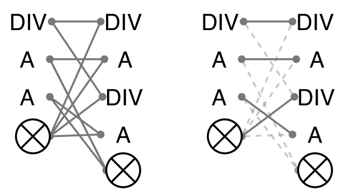
Figure 2. From the input trees depicted in Figure 1, we build a bipartite graph $G$ representing the set of all possible matching (left) and then compute the optimal full matching (right).

Given an edge $e(n,m)\in E(G)$ linking $n$ to $m$, FTM defines the cost $c(e)$ to quantify how different $n$ and $m$ are, considering both their labels and the topology of the tree. Starting from the bipartite graph $G$ describing all possible matchings, the idea behind FTM is to compute the costs $c(e)$ of each edge $e\in E(G)$ and to find the optimal matching with respect to costs—i.e., to select the set of edges $M\subset E(G)$, such that $M$ is full and $c(M)$ is minimal (where $c(M)=\sum_{e\in E(G)}c(e)$).

The upper part of the Figure 3 describes the main steps involved in computing the final full matching between $T_{1}$ and $T_{2}$.

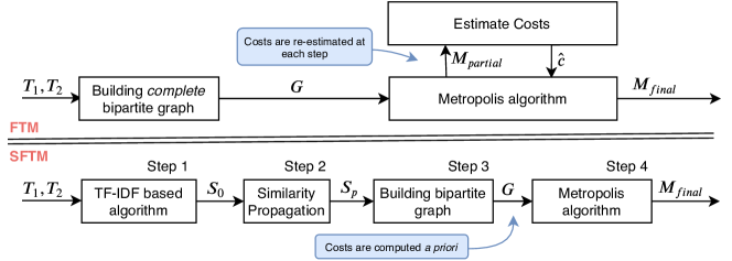
Figure 3. Steps to compute a full matching between two tree $T_{1}$ and $T_{2}$. In the top, we describe FTM and in the bottom, our algorithm: SFTM

3.1. Cost Estimation

As FTM provides a wide flexibility regarding possible matchings, the design of the cost function is a key parameter in order to obtain a matching that takes into account both the labels and the topology of the trees. Typically, the cost of an edge $e$ between two nodes $n$ and $m$ is computed as follows:

(1) $$c(e)=\begin{cases}w_{n}&\text{if}\ n\ or\ m\in\{\Theta_{1},\Theta_{2}\}\\ w_{r}c_{r}(e)+w_{a}c_{a}(e)+w_{s}c_{s}(e)&\text{otherwise}\end{cases}$$

where $\Theta_{1},\Theta_{2}$ are no-match nodes, $w_{n}$ is the penalty when failing to match one of the edge ends, $c_{r}$, $c_{a}$ and $c_{s}$ are the cost of relabeling, violating ancestry relationship and violating sibling group, respectively, and $w_{r}$, $w_{r}$ and $w_{r}$ their associated weight in the cost function. $w_{n},w_{r},c_{r},w_{a}$ and $w_{s}$ are parameters of the cost function that depend on the kind of matching the user requires. By extension, we note $c(M)=\sum_{e\in M}c(e)$ the cost of a matching $M$.

Given $e(n,m)$, the ancestry and sibling costs, $c_{a}(e)$ and $c_{s}(e)$, model the changes in topology that matching $n$ with $m$ entails. Unfortunately, we can only compute the costs $c_{a}$ and $c_{s}$ if we have access to a full matching, as both costs require a knowledge on how other nodes in the tree were matched (e.g., $c_{a}$ involves counting the number of children of $n$ matched with nodes that are not children of $m$). In order to circumvent the problem, FTM defines the approximate costs $\hat{c_{a}},\hat{c_{s}}$ that can be computed from bounds on the different components of the cost $c$. Practically, in order to generate one possible full matching, FTM iteratively selects edges in $G$ and, each time an edge is selected, the bounds of $c$ are tightened (we can approximate $c$ more precisely), which means the costs $\hat{c_{a}},\hat{c_{s}}$ must be recomputed. This is illustrated in the upper part of Figure 3.

The need to recompute the approximated costs after each edge selection therefore imposes some critical limitation on the scalability of the algorithm.

3.2. Metropolis Algorithm

Finding the optimal matching, given the graph $G$ and the cost function $c$ is a challenging problem, the authors even proved in (Kumar et al., 2011b) that the problem is NP-hard. Consequently, the authors described how to use the Metropolis algorithm (Metropolis et al., 1953) to approximate the optimal matching. The Metropolis algorithm provides a way to explore a probability distribution by random walking through samples. FTM uses this algorithm to random walk through several full matchings, and select the least costly. The algorithm needs to be configured with:

1. An initial sample (full matching) $M_{0}$,

2. A suggestion function $M_{t}\mapsto M_{t+1}$,

3. An objective function to maximize: $f:M\mapsto\text{quality of }M$,

4. The number of random walks before returning the best value.

Kumar et al. defines the objective function $f$ by:

(2) $$f_{FTM}(M)=\exp(-\beta\ c(M))$$

In order to suggest a matching $M_{t+1}$ from a previously accepted one $M_{t}$, FTM selects a random number of edges from $M_{t}$ to keep, sorts remaining edges by increasing costs and iterate through the ordered edges with a chance $\gamma$ to select it. Once an edge $e(n,m)$ is selected, all edges connected to $n$ and $m$ are removed from $G$, approximate costs need to be recomputed for all edges and sorted so we can select another edge. The process is repeated until a full matching is obtained.

Despite using the Metropolis algorithm to reduce the time complexity of the problem, the overall algorithm remains prohibitively costly to compute (cf. Section 5), notably due to the continuous computation of the approximated cost for each step of the full matching generation.

3.3. Complexity Analysis

The original FTM paper (Kumar et al., 2011b) does not provide any information on the complexity or the computation time of the algorithm. We provide an analysis of FTM’s theoretical complexity to use as a baseline to our approach (SFTM).

Complete bipartite graph $G$

Building the complete bipartite graph requires linking each node form $T_{1}$ to each node from $T_{2}$, which requires $O(N^{2})$ operations.

Metropolis Algorithm

For each iteration of the Metropolis algorithm, FTM needs to suggest a new matching. In the worst case, the algorithm should choose among all $N^{2}$ edges. Each time an edge between $e_{1}$ and $e_{2}$ is selected, all other edges connected to $e_{1}$ and $e_{2}$ are pruned and costs a re-estimated. It means that costs need to be re-computed and sorted for $N^{2}$ edges, then $(N-1)^{2}$ edges (after selection and pruning) and so on until all edges have been selected or pruned. This implies that the total number of times the costs are re-computed and sorted is in $O(\sum^{N}_{n=0}n^{2})$ = $O(N^{3})$. Computing the cost for a given edge linking $e_{1}$ and $e_{2}$ involves counting the number of potential ancestry and sibling violations, which requires going through all edges connected to siblings and children of $e_{1}$ and $e_{2}$. Even if we assume the number of siblings and children is independent of $N$, it still means estimating the cost of one edge requires $O(N)$ operations. Thus, in the worst case, the amount of operations done by FTM for each iteration of the Metropolis algorithm is in $O(\sum^{N}_{n=0}n^{3})$ = $O(N^{4})$ (using Faulhaber’s Formula).

4. Similarity-based Flexible Tree Matching

Similarity-based Flexible Tree Matching (SFTM) replaces the cost system of FTM by a similarity-based cost that can be computed a priori. This approach drastically improves computation times and exposes a parameter that can be tuned to find the desired trade-off between computation time and matching accuracy.

Given two trees $T_{1}$ and $T_{2}$, SFTM relies on the creation of a similarity metric between the nodes of $T_{1}$ and $T_{2}$. We compute this similarity metric for all pairs of nodes using i) inverted indices for labels and ii) label propagation for the topology. We build a bipartite graph $G$ using this similarity metric to compute the costs and apply the Metropolis algorithm to approximate the optimal full matching from $G$. This new similarity measure allows us to improve the FTM algorithm in two key aspects:

1. When building $G$, we do not create all $N^{2}$ possible edges. We only consider edges linking two nodes with a non-null similarity.

2. When generating a full matching, we never need to recompute the costs since these costs are solely dependant on our similarity measure.

In this section, we (a) introduce our new similarity metric and (b) describe how we leverage it to approximate the optimal full matching.

4.1. Node Similarity

The similarity metric between nodes from $T_{1}$ and $T_{2}$ is computed in two steps: (1) we compute $S_{0}$, the initial similarity function using only labels of the trees individually, and then (2) we transform $S_{0}$ to take into account the topology of the tree and compute our final similarity function $S_{p}$. The computation of $S_{0}$ leverages inverted index techniques traditionally used to query text in a large document databases. In our case, documents we query against are nodes from $T_{1}$ and queries are extracted from $T_{2}$ nodes.

4.1.1. Initial Similarity (step 1)

To compute the initial similarity $S_{0}$ (step 1 in Figure 3) between $T_{1}$ and $T_{2}$, we independently compare the labels of $T_{1}$ and $T_{2}$ using TF-IDF. The resulting initial similarity $S_{0}$ does not take the topology of the trees into account.

In order to take into account relabeling cost between nodes, FTM and TED allow the user to input a pairwise comparison function $label(n),label(m)\mapsto similarity\ score$. Computing this similarity score for all the pairs of nodes requires $O(N^{2})$ operations. To reduce the number of operations, SFTM uses—instead—inverted indices: we require the user to input a $tokenize:n\mapsto\ token\ list$ function, and then (1) we sort each node $n$ from $T_{1}$ into a set of tokens (as defined by the $tokenize$ function), before (2) we iterate through tokens of nodes $m$ from $T_{2}$ and increase the value of $S_{0}(n,m)$ for each token $n$ and $m$ have in common. Section 4.2.2 provides a detailed description of the $tokenize$ function we use in our evaluation.

After sorting nodes $n$ from $T_{1}$ into tokens, we obtain an inverted index $T_{map}$ (for Token Map), which is a table where each entry contains one token $t$ along with the list of nodes that contains the token.

The idea behind the inverted index $T_{map}$ is to use the information that a node $n\in T_{1}$ belongs to a token as a differentiating feature of $n$ allowing to compare it to nodes $m\in T_{2}$. If a token contains all nodes in $T_{1}$, this token has no differentiating power. In general, the rarest a token, the more differentiating it is. This idea is very common in Natural Language Processing (NLP) and a common tool to measure how rare is a token is TF-IDF and more precisely, the Inverted Document Frequency (IDF) part of the formula.

Applying TF-IDF to our similarity yields the following definition:

(3) $$IDF(t) =log(|T_{1}|/|T_{map}[t]|)$$

(4) $$S_{0}(n,m) =\sum_{t\in tk(n)\cap tk(m)}IDF(t)$$

The Inverted Document Frequency function (IDF) is a measure of how rare a token is, $|T_{map}[t]|$ is the number of nodes containing the token $t$ and $tk$ is a short for the user input $tokenize$ function. Intuitively, we retrieve all common tokens between $n$ and $m$, and for each common token $t$, we increase $S(n,m)$ by a high value if $t$ is rare and a low value if $t$ is common. In Section 4.2, we give a detailed implementation of how to compute the initial similarity $S_{0}$.

Tokens that appear in many nodes have little impact on the final score (i.e., low IDF) yet have a very negative impact on the computation time. In our algorithm, we expose the sublinear threshold function $f:N\mapsto f(N)<N$ as a parameter of the algorithm. We use $f$ to filter out all tokens appearing in more than $f(N)$ nodes. $f$ defines a threshold between computation time and matching quality: when $N-f(N)$ decreases, computation times and matching quality increase. In Section 4.3, we discuss how $f(N)$ influences the worst-case theoretical complexity.

4.1.2. Local Topology (step 2)

$S_{0}$ represents the similarity between node labels, but does not take into account the topology of the trees. To weight in local topology similarities, we propagate the score of each node couple to their offspring. This idea of propagation is inspired by recent Graph Convolutional Network (GCN) techniques (Kipf and Welling, 2016).

The original FTM algorithm includes two terms in the cost function, $c_{a}$ and $c_{s}$, which reflect the topology of the trees. Since we do not use these terms, we need our similarity to reflect both the similarity of node labels and the similarity of the local topology. We first compute the score matrix $S_{0}$, based on the label similarity we described above, then we update our score to take into account the matching score of the parents of $n$ and $m$.

That way, $n$ will have a higher similarity score with $m$ if their respective parents are also similar. We repeat the process $p$ times ($p$ for propagation) until we obtain a score function $S_{p}$ that reflects both the label similarity and the local topology similarity:

(5) $$S_{p}(n,m)=\sum_{i=0}^{p}w_{i}S_{0}(parent^{i}(n),parent^{i}(m))$$

where $parent^{i}(n)$ is the $i^{th}$ parent of $n$ (with $parent^{0}(n)=n$) and $w_{0},w_{1}\dots w_{p}$ are weights. In practice, to limit the complexity, we only compute $S_{p}$ for all couples that have a non-null initial score: $\{(n,m)\in T_{1}\times T_{2}|S_{0}\neq 0\}$.

4.1.3. Building the bipartite graph $G$ (step 3)

Using our final score function $S_{p}$, we can now build the bipartite graph $G$: we iterate on all nodes $n\in T_{1}$ and we create an edge $e(n,m)$ for each node $m\in T_{2}$ where $S_{p}(n,m)\neq 0$ and associate it with the cost $c(n,m)=1/(1+S_{p}(n,m))$. Our resulting cost function is thus defined as follows:

(6) $$c_{SFTM}(e)=\begin{cases}w_{n},&\text{if }n_{1}\text{ or }n_{2}\text{ is a no-match node}\\ \frac{1}{1+S_{p}(n,m)},&\text{otherwise}\end{cases}$$

Importantly, unlike the bipartite graph built in the FTM algorithm, the resulting bipartite graph $G_{SFTM}$ is not complete as only edges such that $S_{p}(n,m)\neq 0$ are considered. This is one of the key differences allowing to improve computation times.

4.2. Implementation Details

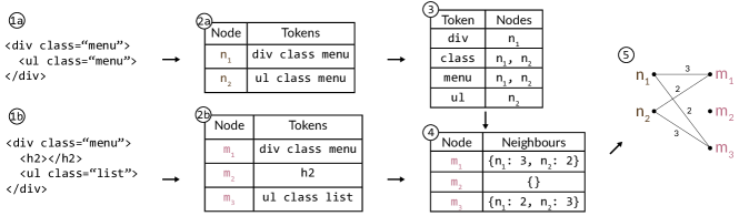
Figure 4. Creating the bipartite graph $G$ from two example DOMs. (1a,b) are the input DOMs, (2a,b) the extracted tokens, (3) the inverted index $T_{map}$ , (4) the neighbours dictionaries and (5) the bipartite graph $G$. For simplicity, the figure shows a matching where IDF(t) = 1 , $p=0$ and no-match nodes are not displayed.

In the previous section, we introduced SFTM algorithm and described how it compares to FTM. In this section, we describe more precisely how we implement the different steps of SFTM.

4.2.1. Node Similarity (step 1 and 2)

Let us consider two trees $T_{1}$ and $T_{2}$. We first build the dictionary $T_{map}$. $T_{map}$ is an inverted index—i.e., each entry of $T_{map}$ is a tuple $(token,nodes)$ where $token$ is a token (usually a string) and $nodes$ is a set of all $n\in T_{1}$ that belongs to $token$. Figure 4 (2a,b) depicts two examples of inverted index. We note $T_{map}[key]$ the set of $nodes$ whose key in $T_{map}$ is $key$. In Section 4.2.2, we further describe how we sort HTML nodes into tokens.

Given the inverted index $T_{map}$, we define the function $IDF:t\mapsto log(N/|T_{map}[t]|)$. In order to limit the complexity of our algorithm, we remove every token $t\in T_{map}$ that is contained by more than $f(N)=\sqrt{N}$ nodes where $f$ is the chosen sublinear threshold function. This is equivalent to putting a threshold on $IDF$ to only keep tokens $\{t\in T_{map}|IDF(t)>log(\sqrt{N})\}$. Removing the most common tokens has a limited impact on matching quality since these are exactly the tokens that provide the least information on the nodes they appear in (see Figure LABEL:sec:parameter).

Input:

m: a node in $T_{2}$

$T_{map}$: token map, dictionary of nodes from $T_{1}$ per token

Result: neighbors: a dictionary of score per node in $T_{1}$

$neighbors\leftarrow new\ Dictionary()$

$tokens\leftarrow tokens(m)$

foreach t in tokens do

       foreach node in $T_{map}$[t] do

             $neighbors[node]+=IDF(t)$

            

       end foreach

      

end foreach

return neighbors

Algorithm 1 For a given node $m\in T_{2}$, compute similarity score $S_{0}(n,m)$ with all $n\in T_{1}$ such that $S_{0}>0$

Once we have the token index $T_{map}$ and $IDF$, we apply Algorithm 1 on each node $m\in T_{2}$. In Algorithm 1, we first compute the tokens of the current node $m$ and for each token $t$, we use $T_{map}$ to retrieve the nodes $n\in T_{1}$ that contain the token $t$. Each node $n$ thus retrieved is a neighbor of $m$—i.e., $S_{0}(n,m)\neq 0$. Finally, for each neighbour $n$ of $m$, we add $IDF(t)$ to the current score $S_{0}(n,m)$. At this point, we have a $neighbors(m)$ dictionary for each node $m\in T_{2}$. Each $neighbors(m)$ dictionary contains all non-null matching scores: $\forall n\in keys(neighbors(m)),neighbors(m)[n]=S_{0}(n,m)$. Using the formula 5, we can now easily compute $S_{p}$.

4.2.2. Building the Token Vector

The way we choose to compute the tokens contained in a node $n$ strongly influences the quality of our similarity score. Finding the optimal way to compute these tokens has been the topic of numerous studies  (Christen, 2011; Steorts et al., 2014; Datar et al., 2004). We implemented the following $tokenize$ function to compute the tokens. Given an HTML node $n$:

⬇

<tag a[1]="v[1]" … a[n]="v[n]">

CONTENT

</tag>

Where $p$ is the number of attributes, $(a[i],v[i]),i\in[1,l]$ are the attributes of $n$ and their associated values. The absolute XPath of $n$ is $xPath(n)$, we say that $n$ contains the following tokens:

(7) $$tokenize(n)=\{tag,a[1]...a[l],tk(v[1])...tk(v[l]),xPath(n)\}$$

where $tk$ is a standard string tokenizer function that takes a string and divides it into a list of tokens by splitting it on each non Latin character.

The absolute XPath of a node $n$ in a DOM is the full path from the root to the element where ranks of the nodes are indicated when necessary—e.g., html/body/div[2]/p.

4.2.3. Building G (step 3)

Using Equation 6, we compute the cost $c(n,m)$ for each couple $(n,m)$ where $S_{p}(n,m)\neq 0$. Then, for each node $m\in T_{2}$, we add one edge for all nodes $neighbours(m)\in T_{1}$ .

4.2.4. Metropolis Algorithm (step 4)

Once we built the graph $G$ with its associated costs, we need to find the set of edges $M$ in $G$ that constitutes the best full matching. In order to do so, we use the same technique as FTM. But, when it comes to applying the Metropolis algorithm, SFTM differentiates from FTM in two ways: (1) we modified the objective function and (2) SFTM matching suggestion function is faster to compute since costs never need to be recomputed.

FTM uses the objective function $f_{FTM}(M)=\exp(-\beta\ c(M))$. In the original FTM paper, the authors noted that the parameter $\beta$ seemed to depend on $|M|$. In order to avoid this dependency, we normalize the total cost:

(8) $$f_{SFTM}(M)=\exp(-\beta\ \frac{c(M)}{|M|})$$

The function $suggestMatching:M_{t}\mapsto M_{t+1}$ takes a full matching $M_{t}$ and returns a full matching $M_{t+1}$ related to $M_{t}$. In the following Algorithm 2,

1. $selectEdgeFrom(edges)$ loops through $edges$ (in order) and at each iteration $i$, has a chance $\gamma\in[0,1]$ to stop and return $edges[i]$,

2. $connectedEdges(edge)$, where $edge$ connects $u$ and $v$, returns the set $E$ of all edges connected to $u$ or $v$ (note that $edge\in E$).

Data: $G$ : The bipartite graph

Input: $M_{t}$: A full matching

Result: $M_{t+1}$: the suggested full matching

$M_{t+1}\leftarrow[]$

$remainingEdges\leftarrow sortedEdges(G)$

$toKeep\leftarrow randomInt(0,|M_{t}|)$

for i = 0 .. toKeep do

       $M_{t+1}$.add(edge)

       remainingEdges.removeAll(connectedEdges(edge))

end for

while $remainingEdges$ is not empty do

       $edge\leftarrow SelectEdgeFrom(remainingEdges)$

       $M_{t+1}$.add(edge)

       remainingEdges.removeAll(connectedEdges(edge))

end while

return $M_{t+1}$

Algorithm 2 Suggest a new matching

In practice, we first compute all the connected nodes and edges before storing them as dictionaries, so that the function $connectedEdges$ in Algorithm 2 can be computed in $O(1)$ time. It is worth noting that, to allow fast removal, the list $remainingEdges$ is implemented as a double-linked list. The parameter $\gamma$ defines a trade-off between exploration (low $\gamma$) and exploitation (high $\gamma$).

4.3. Complexity Analysis

We are interested in evaluating the time complexity of the algorithm with respect to $N$. In our analysis, we consider that $n_{t}$, the maximum number of tokens per node is a constant since it does not evolve with $N$.

When building $G$, we first compute the inverted index $T_{map}$. Computing $T_{map}$ requires to iterate through tokens of all nodes in $T_{1}$, which implies a complexity in $O(N\cdot n_{t})=O(N)$.

To find the neighbours of nodes from $T_{2}$ using $T_{map}$, we iterate through all the nodes in $T_{2}$. Each node in $T_{2}$ has $n_{t}$ tokens. The number of nodes containing a token is artificially limited to $f(N)$. Thus, building the similarity function $S_{0}$ takes $O(N\cdot f(N))$ time.

For each $m\in T_{2}$, we create an edge for each neighbor $n\in T_{1}$. Each token $t\in m$ adds up to $f(N)$ neighbors. It means that the total number of edges is in $O(N\cdot n_{t}\cdot f(N))$ = $O(N\cdot f(N))$.

Before executing the Metropolis algorithm on $G$, we sort the edges by cost, which takes $O(N\cdot f(N)\cdot log(N\cdot f(N)))=O(N\cdot f(N)\cdot log(N))$ (as $f(N)\leq N$). Finally, at each step of the Metropolis algorithm, we run the $suggestMatching$ function, which prunes a maximum of $O(f(N))$ neighbors for each one of the $N$ edges it selects.

Overall, sorting all edges requires the highest theoretical complexity: $O(N\cdot f(N)\cdot log(N))$. If no threshold is set—i.e. $f(N)=N$—then the overall complexity of SFTM is $O(N^{2}\cdot log(N))$, which keeps outperforming the TED ($O(N^{3})$) and FTM ($O(N^{4})$).

In the evaluation, we used $f(N)=\sqrt{N}$ which leads to a complexity in $O(N\cdot\sqrt{N}\cdot log(N))$. The empirical evaluation conducted in Section 5 tend to suggest that our analysis might be too pessimistic.

5. Empirical Evaluation

The objective of this evaluation is to assess that:

1. The quality of the matchings computed by SFTM compares with the baseline APTED,

2. The SFTM algorithm offers practical speed gains on real-life web documents.

5.1. Input Web Document Dataset

We need to assess the ability of SFTM to match the nodes between two slightly different DOM $D$ and $D^{\prime}$.

DOM mutation.

To build a dataset of $(D,D^{\prime})$ tuples where the ground truth (perfect matching) is known, we developed a mutation-based tool that works the following way:

1. We construct the DOM $D$ from an input web document,

2. For each element of $D$, we generate a unique signature attribute,

3. For each original DOM $D$, we randomly generate a set of mutated versions: the mutants. Each mutant $D^{\prime}$ is stored along with the precisely described set of mutations that was applied to $D$ to obtain $D^{\prime}$. Importantly, the signature tags of the elements in $D$ are transferred to $D^{\prime}$, which constitutes the perfect matching between $D$ and $D^{\prime}$.

In our tool, most attention has been dedicated to the choice of relevant mutations to apply. The following table summarizes the set of relevant mutations possibly applied to an element of the DOM.

Element	Mutation operators
Structure	remove, duplicate, wrap, unwrap, swap
Attribute	remove, remove words
Content	replace with random text, change letters,
	remove, remove words

Baseline algorithms.

We compare SFTM to APTED, which is the reference implementation of TED that yields the best performance so far. The implementation of APTED used for the evaluation is the one provided by the authors of (Pawlik and Augsten, 2016, 2015). We consider the pairs $(D,D^{\prime})$ taken from the above web document dataset, and we ran SFTM and APTED algorithms with each pair to match $D$ with $D^{\prime}$ on the same machine.

Input document sample.

We fed our mutation tool with the home pages of the Top 1K Alexa websites. For each DOM $D$ thus retrieved, we created 10 mutants $D^{\prime}$ with a number of mutated nodes ranging from $0$ to $50\%$ of the total number of nodes on the page.

Overall, we considered an input dataset composed of $7,502$ document tuples. We ran SFTM on the complete dataset but, due to high computation times, APTED can only be evaluated on a subset of this dataset comprising $852$ tuple documents, which represents a 3 % error margin with 95 % confidence with respect to the complete dataset. Figures 6 and 7 comparing APTED and SFTM are based on this partial dataset, while the complete dataset was used when studying SFTM in isolation (cf. Figure 8). Figure 5 reports on the size distribution, in number of nodes, of the selected web documents for both complete and partial datasets.

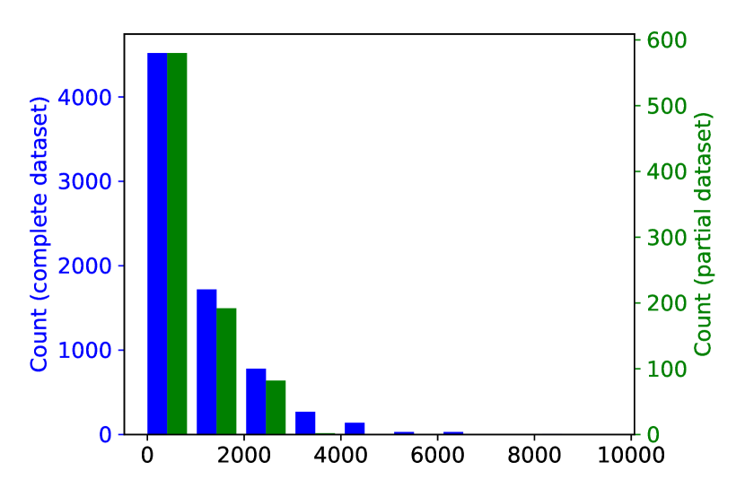
Figure 5. The distribution of DOM sizes (in terms of nodes) for the complete (left, blue) and the partial (right, green) datasets.

Ground truth.

When building the dataset, we keep track of nodes’ signature so that we always know which nodes from $D$ should match with nodes from $D^{\prime}$. This ground truth is ignored by the evaluated algorithms, but is used a posteriori to measure and compare the quality of the matchings computed by the algorithms under evaluation.

5.2. Experimental Results

Matching quality.

The signature tags on nodes from $D$ and $D^{\prime}$ allow us to judge the quality of the matching according to two metrics: (1) mismatch, the number of nodes couples that were wrongly matched and (2) no-match, the number of nodes from $D$ that were matched with no nodes from $D^{\prime}$. We call successful match rate, the number of couples rightfully matched by the algorithm—i.e., that is neither a mismatch nor a no-match. The list of possible mutations between $D$ and $D^{\prime}$ include the removal of a node. In case we remove a node, the algorithms will (legitimately) not be able to match the removed nodes. We call optimal successful match rate, the maximum ratio of nodes that the algorithms can successfully match: $\frac{total\ nodes\ in\ D-number\ of\ removals\ in\ D^{\prime}}{total\ nodes\ in\ D}$. To measure the quality of the matchings, we compare the successful match rate of the matchings computed by both algorithms with the optimal successful match rate on Figure 6.

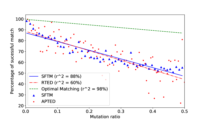
Figure 6. Successful match rate according to mutation ratio for SFTM and APTED

We observe that SFTM and APTED have very similar performance. They both seem to perform linearly with the number of mutations. However, APTED is much less stable than SFTM with a correlation coefficient $r^{2}=60\%$.

Completion time.

For each couple ($D$, $D^{\prime}$) retrieved from the dataset, we measured the time taken by SFTM and APTED to compute a matching. For practical reasons, we set a timeout to APTED computations at 7 minutes (450 seconds). Figure 7 reports on the average time (in seconds) to match DOM couples of increasing size (in terms of number of nodes) for both algorithms. We note that APTED computation time varies greatly depending on the DOM couple. While the theoretical worst case complexity of APTED is $O(n^{3})$, we can observe in practice that APTED may run up to 100 times slower than SFTM.

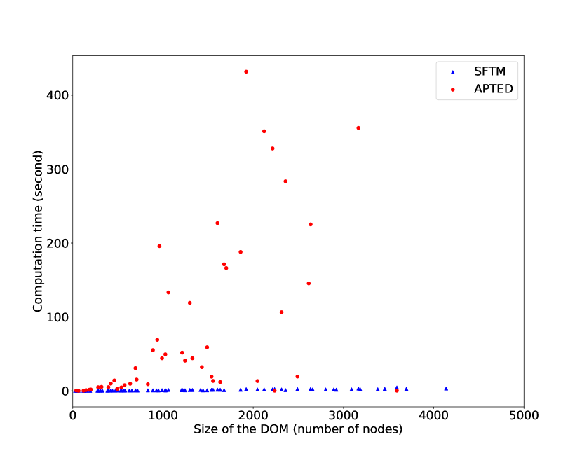
Figure 7. Average time to compute matching by DOM size for APTED and SFTM. APTED computation timeout has been set at 450 seconds

Figure 8 delivers a closer look on the scalability of SFTM. The empirical results seem to indicate an evolution in $O(n\cdot log(n))$: in Figure 8, we replaced the X axis from the number of nodes in the DOM $n$ to $n\ log(n)$ then computed a linear regression on the curve which resulted in a correlation coefficient $r^{2}=86\%$.

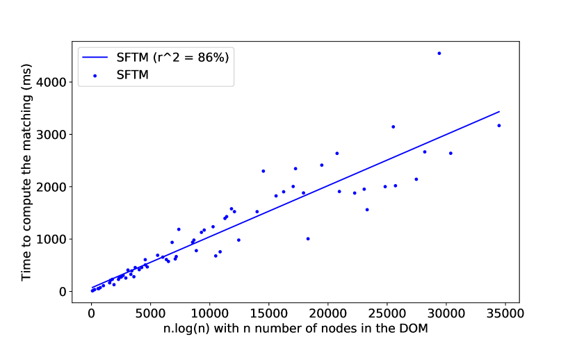
Figure 8. Average time to compute matching by $n\ log(n)$ value for SFTM, with $n$ the number of nodes in the DOM

This observation raises the question of the impact of the sublinear threshold function $f$ on the performance of SFTM. We therefore conducted a sensitivity analysis of this parameter to better understand potential trade-offs offered by the definition of this function, with regards to the complexity analysis we performed (cf. Section 4.3).

Parameter sensitivity.

Since we aim at improving the performances of SFTM in term of computation times, we study the sensitivity of the sublinear threshold function $f$ which is a parameter that directly influences the computation time of the algorithm.

Figure 9 reports on the evolution of SFTM performances when $f$ varies. To study the sensitivity of $f$, we choose to use the power function $f(N)=N^{\alpha}$ as a threshold and display how the computation times and matching accuracy evolve with $\alpha$.

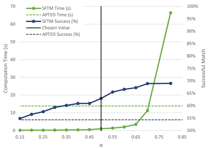
Figure 9. Performance of SFTM given $f(N)=N^{\alpha}$ according to $\alpha$. APTED performance on the same dataset is shown as a reference

For this experiment, as we are interested in studying the sensitivity of the $\alpha$ parameter on the performances of SFTM, we consider a subset of $53$ tuples from the complete dataset used in previous sections (cf. Section 5.2), which represents a 13.4 % error margin with 95 % confidence. On average, on this subset, DOM trees contain $1,065$ nodes and mutants have a $22\%$ mutation ratio, which remains representative of the complexity of web documents considered in this paper.

As expected, when $\alpha$ increases, the quality of the matching and the computation times increase. However, beyond a certain value of $\alpha$, the increase of computation time is significantly superior to the gain in accuracy: increasing $\alpha$ from $0.5$ to $0.8$ entails more than 60 times longer computation times for only $3.5\%$ gain in accuracy. Intuitively, this is because tokens contained in most nodes provide very few information (low Inverse Document Frequency), but increase the complexity quadratically. In this paper, we used $\alpha=0.5$ (i.e., $f(N)=\sqrt{N}$): this value achieves good enough performances to demonstrate that SFTM can match two real-life web documents in practical time without compromising on quality.

6. Threats to Validity

The absolute values of completion times depend on the machine on which the algorithms were executed. As computations took time, we had to run both SFTM and APTED on a server, which is shared among several users. Although we paid a careful attention to isolate our benchmarks, the available resources of the server might have varied along execution thus impacting our results. Nevertheless, the repetition of measures reports a clear signal in favour of SFTM.

Our dataset contains the homepages of the Top 1k Alexa websites. The fact that our qualitative evaluation has only been conducted on homepages might have biased the results since such pages might not be fully representative of the complexity of online documents.

We evaluated the quality of the matchings using synthetic mutations on real-life websites. We dedicated a lot of thought into choosing an objective set of potential mutations representative of real-life evolution of websites. However, there is still a chance we missed some common mutations to which SFTM might prove to be not robust.

7. Conclusion & Perspectives

Comparing modern real-life web documents is a challenge for which traditional Tree Edit Distance (TED) solutions are too restricted and computationally expensive. (Kumar et al., 2011b) introduced Flexible Tree Matching (FTM) to offer a restriction-free matching, but at the cost of prohibitive computational times. In this paper, we presented Similarity-based Flexible Tree Matching (SFTM), which extends FTM to offer tractable computational times while offering non-restricted matching. We evaluated our solution using mutations on real-life documents and we showed that SFTM qualitatively compares to TED while improving the performances by two orders of magnitude. The proof of concept we deliver demonstrates that matching real-life web documents in practical time is possible.

We believe that having a robust algorithm to efficiently compare web documents will open up new perspectives within the web community. In future work, we will further investigate on how to improve the quality of the matchings by analyzing which situations cause SFTM to make mistakes in order to establish guidelines to adjust the exposed parameters.

Whether our work might be applicable to other trees than web DOMs remains to be tested. Indeed, SFTM strongly relies on the fact that node labels in DOMs are highly differentiating (many specific attributes on each element), which is not the case for all kinds of trees.

References

- (1)
- Bringmann et al. (2018) Karl Bringmann, Paweł Gawrychowski, Shay Mozes, and Oren Weimann. 2018. Tree edit distance cannot be computed in strongly subcubic time (unless APSP can). In Proceedings of the Twenty-Ninth Annual ACM-SIAM Symposium on Discrete Algorithms. Society for Industrial and Applied Mathematics, 1190–1206.
- Choudhary et al. (2011) Shauvik Roy Choudhary, Dan Zhao, Husayn Versee, and Alessandro Orso. 2011. Water: Web application test repair. In Proceedings of the First International Workshop on End-to-End Test Script Engineering. ACM, 24–29.
- Christen (2011) Peter Christen. 2011. A survey of indexing techniques for scalable record linkage and deduplication. IEEE transactions on knowledge and data engineering 24, 9 (2011), 1537–1555.
- Datar et al. (2004) Mayur Datar, Nicole Immorlica, Piotr Indyk, and Vahab S Mirrokni. 2004. Locality-sensitive hashing scheme based on p-stable distributions. In Proceedings of the twentieth annual symposium on Computational geometry. ACM, 253–262.
- Fokaefs et al. (2011) Marios Fokaefs, Rimon Mikhaiel, Nikolaos Tsantalis, Eleni Stroulia, and Alex Lau. 2011. An empirical study on web service evolution. In 2011 IEEE International Conference on Web Services. IEEE, 49–56.
- Hao and Zhang (2007) Yanan Hao and Yanchun Zhang. 2007. Web services discovery based on schema matching. In Proceedings of the thirtieth Australasian conference on Computer science-Volume 62. Australian Computer society, Inc., 107–113.
- Jiang et al. (1994) Tao Jiang, Lusheng Wang, and Kaizhong Zhang. 1994. Alignment of trees—an alternative to tree edit. In Annual Symposium on Combinatorial Pattern Matching. Springer, 75–86.
- Kipf and Welling (2016) Thomas N Kipf and Max Welling. 2016. Semi-supervised classification with graph convolutional networks. arXiv preprint arXiv:1609.02907 (2016).
- Kumar et al. (2011a) Ranjitha Kumar, Jerry O Talton, Salman Ahmad, and Scott R Klemmer. 2011a. Bricolage: example-based retargeting for web design. In Proceedings of the SIGCHI Conference on Human Factors in Computing Systems. ACM, 2197–2206.
- Kumar et al. (2011b) Ranjitha Kumar, Jerry O. Talton, Salman Ahmad, Tim Roughgarden, and Scott R. Klemmer. 2011b. Flexible tree matching. In Proceedings of the Twenty-Second International Joint Conference on Artificial Intelligence (AAAI).
- Metropolis et al. (1953) Nicholas Metropolis, Arianna W Rosenbluth, Marshall N Rosenbluth, Augusta H Teller, and Edward Teller. 1953. Equation of state calculations by fast computing machines. The journal of chemical physics 21, 6 (1953), 1087–1092.
- Pawlik and Augsten (2011) Mateusz Pawlik and Nikolaus Augsten. 2011. RTED: a robust algorithm for the tree edit distance. Proceedings of the VLDB Endowment 5, 4 (2011), 334–345.
- Pawlik and Augsten (2015) Mateusz Pawlik and Nikolaus Augsten. 2015. Efficient computation of the tree edit distance. ACM Transactions on Database Systems (TODS) 40, 1 (2015), 1–40.
- Pawlik and Augsten (2016) Mateusz Pawlik and Nikolaus Augsten. 2016. Tree edit distance: Robust and memory-efficient. Information Systems 56 (2016), 157–173.
- Reis et al. (2004) Davi de Castro Reis, Paulo Braz Golgher, Altigran Soares Silva, and AlbertoF Laender. 2004. Automatic web news extraction using tree edit distance. In Proceedings of the 13th international conference on World Wide Web. ACM, 502–511.
- Selkow (1977) Stanley M Selkow. 1977. The tree-to-tree editing problem. Information processing letters 6, 6 (1977), 184–186.
- Steorts et al. (2014) Rebecca C Steorts, Samuel L Ventura, Mauricio Sadinle, and Stephen E Fienberg. 2014. A comparison of blocking methods for record linkage. In International Conference on Privacy in Statistical Databases. Springer, 253–268.
- Stocco et al. (2017) Andrea Stocco, Maurizio Leotta, Filippo Ricca, and Paolo Tonella. 2017. APOGEN: automatic page object generator for web testing. Software Quality Journal 25, 3 (2017), 1007–1039.
- Tai (1979) Kuo-Chung Tai. 1979. The tree-to-tree correction problem. Journal of the ACM (JACM) 26, 3 (1979), 422–433.
- Valiente (2001) Gabriel Valiente. 2001. An Efficient Bottom-Up Distance between Trees.. In spire. 212–219.
- Yao et al. (2013) Xuchen Yao, Benjamin Van Durme, Chris Callison-Burch, and Peter Clark. 2013. Answer extraction as sequence tagging with tree edit distance. In Proceedings of the 2013 conference of the North American chapter of the association for computational linguistics: human language technologies. 858–867.
- Zhai and Liu (2005) Yanhong Zhai and Bing Liu. 2005. Web data extraction based on partial tree alignment. In Proceedings of the 14th international conference on World Wide Web. ACM, 76–85.
- Zhang (1995) Kaizhong Zhang. 1995. Algorithms for the constrained editing distance between ordered labeled trees and related problems. Pattern recognition 28, 3 (1995), 463–474.
- Zhang (1996) Kaizhong Zhang. 1996. A constrained edit distance between unordered labeled trees. Algorithmica 15, 3 (1996), 205–222.