Fractional SIS epidemic models

Caterina Balzotti Department of Basic and Applied Sciences for Engineering, Sapienza University of Rome, Via A. Scarpa 16, Rome, Italy (caterina.balzotti@sbai.uniroma1.it, paola.loreti@uniroma1.it )    Mirko D’Ovidio Department of Basic and Applied Sciences for Engineering, Sapienza University of Rome, Via A. Scarpa 10, Rome, Italy (mirko.dovidio@uniroma1.it): corresponding author.    Paola Loreti11footnotemark: 1
Abstract

In this paper we consider the fractional SIS epidemic model (α𝛼\alpha-SIS model) in the case of constant population size. We provide a representation of the explicit solution to the fractional model and we illustrate the results by numerical schemes. A comparison with the limit case when the fractional order α1𝛼1\alpha\uparrow 1 (the SIS model) is also given. We analyse the effects of the fractional derivatives by comparing the SIS and the α𝛼\alpha-SIS models.

Keywords.

α𝛼\alpha-SIS model, SIS model, epidemic models, fractional logistic equation.

Mathematics Subject Classification.

92D30, 78A70, 26A33.

Introduction

The study of mathematical models for epidemiology has a long history, dating back to the early 1900s with the theory developed by Kermack and McKendrick [11]. Such theory describes compartmental models, where the population is divided into groups depending on the state of individuals with respect to disease, distinguishing between groups. The dynamic of the disease is then described by a system of ordinary differential equations for each class of individuals. The use of mathematical models for epidemiology is particularly useful to predict the progress of an infection and to take strategy to limit the spread of the disease. In this work we focus on the α𝛼\alpha-SIS (susceptible - infectious - susceptible) epidemiological model. The SIS model has a long history too [10]. It describes the spread of human viruses such as influenza. The SIS model with constant population is particularly appropriate to describe some bacterial agent diseases such as gonorrhea, meningitis and streptococcal sore throat. SIS is a model without immunity, where the individual recovered from the infection comes back into the class of susceptibles.

Statement of the problem

We propose an α𝛼\alpha-SIS model with constant population size. The novelty concerns the SIS equations with the time fractional Caputo derivative in place of time standard derivative and their explicit solutions in terms of Euler’s numbers and Euler’s Gamma functions.

Let us consider the Caputo fractional derivative introduced in (2.1) below. We provide an explicit representation of the solution to

{𝒟tαS(t)=μβS(t)I(t)+γI(t)μS(t)𝒟tαI(t)=βS(t)I(t)γI(t)μI(t)with S(t)+I(t)=N(t)S(0)=S0 and I(0)=I0,casessuperscriptsubscript𝒟𝑡𝛼𝑆𝑡𝜇𝛽𝑆𝑡𝐼𝑡𝛾𝐼𝑡𝜇𝑆𝑡otherwisesuperscriptsubscript𝒟𝑡𝛼𝐼𝑡𝛽𝑆𝑡𝐼𝑡𝛾𝐼𝑡𝜇𝐼𝑡otherwisewith S(t)+I(t)=N(t)S(0)=S0 and I(0)=I0,\begin{split}&\begin{cases}\mathscr{D}_{t}^{\alpha}\mathnormal{S}(t)=\mu-\beta\mathnormal{S}(t)\mathnormal{I}(t)+\gamma\mathnormal{I}(t)-\mu\mathnormal{S}(t)\\ \mathscr{D}_{t}^{\alpha}\mathnormal{I}(t)=\beta\mathnormal{S}(t)\mathnormal{I}(t)-\gamma\mathnormal{I}(t)-\mu\mathnormal{I}(t)\end{cases}\\ &\text{with $\mathnormal{S}(t)+\mathnormal{I}(t)=N(t)$, $\mathnormal{S}(0)=\mathnormal{S}_{0}$ and $\mathnormal{I}(0)=\mathnormal{I}_{0}$,}\end{split}

for the constant population case N(t)=1𝑁𝑡1N(t)=1, tfor-all𝑡\forall\,t, where α(0,1)𝛼01\alpha\in(0,1) is the order of the Caputo fractional derivative, μ𝜇\mu is the birth rate and the death removal rate, β𝛽\beta is the contact rate and γ𝛾\gamma is the recovery removal rate. The unknown functions S(t)𝑆𝑡S(t) and I(t)𝐼𝑡I(t) represent the percentage of susceptible and infected people at time t>0𝑡0t>0 with initial data S0subscript𝑆0S_{0} and I0subscript𝐼0I_{0}. As far as we know, although the numerical literature it is unknown a formula for the solution. By using a series representation for the solution to the fractional logistic equation we may give an explicit formula for the unknown functions S𝑆S and I𝐼I. From the numerical point of view, we validate the goodness of the theoretical formulas by applying two different numerical schemes. Then, we compare the fractional case results (0<α<10𝛼10<\alpha<1) with the well-known standard case taking the limit α1𝛼1\alpha\uparrow 1 and we analyse the effects produced by the fractional derivatives.

Motivations

Let us consider an infective disease which does not confer immunity and which is transmitted through contact between people. We divide the population into two disjoint classes which evolve in time: the susceptibles and the infectives. The first class contains the individuals which are not yet infected but who can contract the disease; the second class contains the infected population which can transmit the disease. The SIS model [10] is a simple disease model without immunity, where the individuals recovered from the infection come back into the class of susceptibles. Such a model is used to describe the dynamic of infections which do not confer a long immunity, as the cold or influenza. Fractional calculus is therefore considered in biological models to take into account macroscopic effect. The use of fractional derivatives in the model means that some global effect may produce slowdown in the process. This is verified and discussed in the validation of the model.

State of the art

The logistic function was introduced by Pierre Francois Verhulst [15] to model the population growth. At the beginning of the process the growth of the population is fast; then, as saturation process begins, the growth slows, and then growth is close to be flat. The problem to give a solution of the fractional logistic equation was unsolved and several attempts have been done (see for instance [7, 3, 16, 17]). Concerning the fractional SIS model, some works can be listed about numerical solutions obtained by considering different methods. From the technical point of view our result take advantage of the explicit representation by series of the solution of fractional logistic equation solved in the recent paper [6]. Thanks to a fruitful formulation of the SIS model we are able to adapt the results obtained for fractional logistic equation in [6] and to give the solution of fractional SIS model by series.

In recent years the study of epidemiological models using fractional calculus has spread widely. In [12] the authors prove via numerical simulations that the proposed fractional model gives better results than the classical theory, when compared to real data. Moreover, for some diseases it is necessary to take into account the history of the system (see for example [14]), thus non-locality and memory become important to model real data. Indeed, fractional operators consider the entire history of the biological process and we are able to model non local effects often encountered in biological phenomena.

Main results

We provide an explicit representation of the solution to

{𝒟tαS(t)=μβS(t)I(t)+γI(t)μS(t)𝒟tαI(t)=βS(t)I(t)γI(t)μI(t)with S(t)+I(t)=1S(0)=S0 and I(0)=I0,casessuperscriptsubscript𝒟𝑡𝛼𝑆𝑡𝜇𝛽𝑆𝑡𝐼𝑡𝛾𝐼𝑡𝜇𝑆𝑡otherwisesuperscriptsubscript𝒟𝑡𝛼𝐼𝑡𝛽𝑆𝑡𝐼𝑡𝛾𝐼𝑡𝜇𝐼𝑡otherwisewith S(t)+I(t)=1S(0)=S0 and I(0)=I0,\begin{split}&\begin{cases}\mathscr{D}_{t}^{\alpha}\mathnormal{S}(t)=\mu-\beta\mathnormal{S}(t)\mathnormal{I}(t)+\gamma\mathnormal{I}(t)-\mu\mathnormal{S}(t)\\ \mathscr{D}_{t}^{\alpha}\mathnormal{I}(t)=\beta\mathnormal{S}(t)\mathnormal{I}(t)-\gamma\mathnormal{I}(t)-\mu\mathnormal{I}(t)\end{cases}\\ &\text{with $\mathnormal{S}(t)+\mathnormal{I}(t)=1$, $\mathnormal{S}(0)=\mathnormal{S}_{0}$ and $\mathnormal{I}(0)=\mathnormal{I}_{0}$,}\end{split} (1.1)

in terms of uniformly convergent series on compact sets.

Let us introduce the basic reproduction number [2] i.e. the expected number of secondary infections produced during the period of infection, which is given by

σ=βγ+μ,𝜎𝛽𝛾𝜇\sigma=\frac{\beta}{\gamma+\mu}, (1.2)

where γ+μ𝛾𝜇\gamma+\mu is the infection period. Let

c=σ1σ𝑐𝜎1𝜎c=\displaystyle\frac{\sigma-1}{\sigma} (1.3)

be the so-called carrying capacity and define b=βc𝑏𝛽𝑐b=\beta c. The problem (1.1) can be solved by considering the fractional logistic equation

𝒟tαI(t)=bI(t)(11cI(t))superscriptsubscript𝒟𝑡𝛼𝐼𝑡𝑏𝐼𝑡11𝑐𝐼𝑡\mathscr{D}_{t}^{\alpha}\mathnormal{I}(t)=b\,I(t)\left(1-\frac{1}{c}I(t)\right) (1.4)

In the following theorems, B(x,y)𝐵𝑥𝑦B(x,y) denotes the Beta function, Γ(x)Γ𝑥\Gamma(x) denotes the Euler Gamma function and Ekαsubscriptsuperscript𝐸𝛼𝑘E^{\alpha}_{k} are the α𝛼\alpha-Euler’s number introduced in [6].

Theorem 1.1.

Let α(0,1)𝛼01\alpha\in(0,1), c0𝑐0c\neq 0 and b1/α<1superscript𝑏1𝛼1b^{1/\alpha}<1. An explicit representation of the solution of the fractional SIS model (1.1) with initial condition I0=c/2subscript𝐼0𝑐2\mathnormal{I}_{0}=c/2 and S0=1I0subscript𝑆01subscript𝐼0\mathnormal{S}_{0}=1-\mathnormal{I}_{0} is given by

I(t)𝐼𝑡\displaystyle\mathnormal{I}(t) =ck0EkαbαktαkΓ(αk+1)absent𝑐subscript𝑘0subscriptsuperscript𝐸𝛼𝑘superscript𝑏𝛼𝑘superscript𝑡𝛼𝑘Γ𝛼𝑘1\displaystyle=c\sum_{k\geq 0}E^{\alpha}_{k}\,b^{\alpha k}\frac{t^{\alpha k}}{\Gamma(\alpha k+1)} (1.5)
S(t)𝑆𝑡\displaystyle\mathnormal{S}(t) =1I(t),absent1𝐼𝑡\displaystyle=1-I(t), (1.6)

with

E0α=12,E1α=E0α(E0α)2formulae-sequencesubscriptsuperscript𝐸𝛼012subscriptsuperscript𝐸𝛼1subscriptsuperscript𝐸𝛼0superscriptsubscriptsuperscript𝐸𝛼02\displaystyle E^{\alpha}_{0}=\frac{1}{2},\qquad E^{\alpha}_{1}=E^{\alpha}_{0}-(E^{\alpha}_{0})^{2}

and k1for-all𝑘1\forall k\geq 1

E2kα=0,E2k+1α=1αk+1i,ji+j=kEiαEjαB(αi+1,αj+1).formulae-sequencesubscriptsuperscript𝐸𝛼2𝑘0subscriptsuperscript𝐸𝛼2𝑘11𝛼𝑘1subscript𝑖𝑗𝑖𝑗𝑘subscriptsuperscript𝐸𝛼𝑖subscriptsuperscript𝐸𝛼𝑗𝐵𝛼𝑖1𝛼𝑗1\displaystyle\displaystyle E^{\alpha}_{2k}=0,\qquad E^{\alpha}_{2k+1}=-\frac{1}{\alpha k+1}\sum_{\begin{subarray}{c}i,j\\ i+j=k\end{subarray}}\frac{E^{\alpha}_{i}E^{\alpha}_{j}}{B(\alpha i+1,\alpha j+1)}.

The series is uniformly convergent on any compact subset K(0,rα)𝐾0subscript𝑟𝛼K\subseteq(0,r_{\alpha}), where

rα=1b1/α(Γ(α+1)Γ(3α+1)Γ(2α+1))12α.subscript𝑟𝛼1superscript𝑏1𝛼superscriptΓ𝛼1Γ3𝛼1Γ2𝛼112𝛼r_{\alpha}=\frac{1}{b^{1/\alpha}}\left(\frac{\Gamma(\alpha+1)\Gamma(3\alpha+1)}{\Gamma(2\alpha+1)}\right)^{\frac{1}{2\alpha}}. (1.7)
Theorem 1.2.

Let α(0,1)𝛼01\alpha\in(0,1), c=0𝑐0c=0. An explicit representation of the solution of the fractional SIS model (1.1) with initial condition I0=1/(2β)subscript𝐼012𝛽\mathnormal{I}_{0}=1/(2\beta) and S0=1I0subscript𝑆01subscript𝐼0\mathnormal{S}_{0}=1-\mathnormal{I}_{0} is given by

I(t)𝐼𝑡\displaystyle\mathnormal{I}(t) =1βk0AkαtαkΓ(αk+1),absent1𝛽subscript𝑘0subscriptsuperscript𝐴𝛼𝑘superscript𝑡𝛼𝑘Γ𝛼𝑘1\displaystyle=\frac{1}{\beta}\sum_{k\geq 0}A^{\alpha}_{k}\frac{t^{\alpha k}}{\Gamma(\alpha k+1)}, (1.8)
S(t)𝑆𝑡\displaystyle\mathnormal{S}(t) =1I(t),absent1𝐼𝑡\displaystyle=1-\mathnormal{I}(t), (1.9)

with A0α=12,A1α=(A0α)2formulae-sequencesubscriptsuperscript𝐴𝛼012subscriptsuperscript𝐴𝛼1superscriptsubscriptsuperscript𝐴𝛼02A^{\alpha}_{0}=\frac{1}{2},\,A^{\alpha}_{1}=-(A^{\alpha}_{0})^{2} and

Ak+1α=1αk+1i,ji+j=kAiαAjαB(αi+1,αj+1)k1.formulae-sequencesubscriptsuperscript𝐴𝛼𝑘11𝛼𝑘1subscript𝑖𝑗𝑖𝑗𝑘subscriptsuperscript𝐴𝛼𝑖subscriptsuperscript𝐴𝛼𝑗𝐵𝛼𝑖1𝛼𝑗1for-all𝑘1A^{\alpha}_{k+1}=-\frac{1}{\alpha k+1}\sum_{\begin{subarray}{c}i,j\\ i+j=k\end{subarray}}\frac{A^{\alpha}_{i}A^{\alpha}_{j}}{B(\alpha i+1,\alpha j+1)}\quad\forall\,k\geq 1.

The series converges uniformly in K(0,rα)𝐾0subscript𝑟𝛼K\subset(0,r_{\alpha}) with rα(1/2)1/αsubscript𝑟𝛼superscript121𝛼r_{\alpha}\leq(1/2)^{1/\alpha}.

Outline

The paper is organized as follows. In Section 2 we introduce the fractional α𝛼\alpha-SIS model with constant population size. In Section 3 we prove the main results of the paper. In Section 4 we validate the model using two numerical schemes and we provide some numerical tests also comparing the α𝛼\alpha-SIS model with the SIS one.

The Settings

The fractional derivatives

Fractional Calculus has a long history. Starting from some works by Leibniz (1695) or Abel (1823), it has been developed up to nowadays. The literature is vast and many definitions of fractional derivatives has been given. We recall the well-known derivatives of Caputo and Riemann-Liouville given by following the definitions we will deal with throughout. The Caputo Derivative of a function u(t)𝑢𝑡u(t) is written as

𝒟tαu(t):=1Γ(1α)0tu(s)(ts)α𝑑s,t>0formulae-sequenceassignsuperscriptsubscript𝒟𝑡𝛼𝑢𝑡1Γ1𝛼superscriptsubscript0𝑡superscript𝑢𝑠superscript𝑡𝑠𝛼differential-d𝑠𝑡0\displaystyle\mathscr{D}_{t}^{\alpha}u(t):=\frac{1}{\Gamma(1-\alpha)}\int_{0}^{t}\frac{u^{\prime}(s)}{(t-s)^{\alpha}}ds,\quad t>0 (2.1)

whereas, the Riemann-Liouville derivative of u(t)𝑢𝑡u(t) is defined as follows

𝒟tαu(t)=1Γ(1α)ddt0tu(s)(ts)α𝑑s.superscriptsubscript𝒟𝑡𝛼𝑢𝑡1Γ1𝛼𝑑𝑑𝑡superscriptsubscript0𝑡𝑢𝑠superscript𝑡𝑠𝛼differential-d𝑠\mathcal{D}_{t}^{\alpha}u(t)=\frac{1}{\Gamma(1-\alpha)}\frac{d}{dt}\int_{0}^{t}\frac{u(s)}{(t-s)^{\alpha}}ds. (2.2)

Notice that, for a<b𝑎𝑏a<b, if uL1(a,b)𝑢superscript𝐿1𝑎𝑏u\in L^{1}(a,b) such that uL1(a,b)superscript𝑢superscript𝐿1𝑎𝑏u^{\prime}\in L^{1}(a,b) and |u(t)|tγ1superscript𝑢𝑡superscript𝑡𝛾1|u^{\prime}(t)|\leq t^{\gamma-1} a.e. with γ>0𝛾0\gamma>0, then we have that for t(a,b)𝑡𝑎𝑏t\in(a,b)

|𝒟tαu(t)|1Γ(1α)0tsγ1(ts)1α1𝑑s=B(γ,1α)Γ(1α)superscriptsubscript𝒟𝑡𝛼𝑢𝑡1Γ1𝛼superscriptsubscript0𝑡superscript𝑠𝛾1superscript𝑡𝑠1𝛼1differential-d𝑠𝐵𝛾1𝛼Γ1𝛼\displaystyle\big{|}\mathscr{D}_{t}^{\alpha}u(t)\big{|}\leq\frac{1}{\Gamma(1-\alpha)}\int_{0}^{t}s^{\gamma-1}(t-s)^{1-\alpha-1}ds=\frac{B(\gamma,1-\alpha)}{\Gamma(1-\alpha)}

where

B(α,β)=Γ(α)Γ(β)Γ(α+β),α>0,β>0formulae-sequence𝐵𝛼𝛽Γ𝛼Γ𝛽Γ𝛼𝛽formulae-sequence𝛼0𝛽0\displaystyle B(\alpha,\beta)=\frac{\Gamma(\alpha)\,\Gamma(\beta)}{\Gamma(\alpha+\beta)},\quad\alpha>0,\;\beta>0

is the Beta function and Γ(α)=0essα1𝑑sΓ𝛼superscriptsubscript0superscript𝑒𝑠superscript𝑠𝛼1differential-d𝑠\Gamma(\alpha)=\int_{0}^{\infty}e^{-s}s^{\alpha-1}ds, α>0𝛼0\alpha>0 is the Euler’s gamma function. The Caputo and the Riemann-Liouville fractional derivatives are linked by the following formula

𝒟tαu(t)=𝒟tαu(t)tαΓ(1α)u(0)=𝒟tα(u(t)u(0))superscriptsubscript𝒟𝑡𝛼𝑢𝑡superscriptsubscript𝒟𝑡𝛼𝑢𝑡superscript𝑡𝛼Γ1𝛼𝑢0superscriptsubscript𝒟𝑡𝛼𝑢𝑡𝑢0\displaystyle\mathscr{D}_{t}^{\alpha}u(t)=\mathcal{D}_{t}^{\alpha}u(t)-\frac{t^{-\alpha}}{\Gamma(1-\alpha)}u(0)=\mathcal{D}_{t}^{\alpha}\big{(}u(t)-u(0)\big{)} (2.3)

which will be useful further on. We list some useful properties of the Caputo derivative:

  1. (P1)

    Let u𝑢u be a constant function. Then 𝒟tαu(t)=0superscriptsubscript𝒟𝑡𝛼𝑢𝑡0\mathscr{D}_{t}^{\alpha}u(t)=0.

  2. (P2)

    Le u:[a,b]:𝑢𝑎𝑏u:[a,b]\to\mathbb{R} such that u(a)=0𝑢𝑎0u(a)=0 and 𝒟tαusuperscriptsubscript𝒟𝑡𝛼𝑢\mathscr{D}_{t}^{\alpha}u, 𝒟tαusuperscriptsubscript𝒟𝑡𝛼𝑢\mathcal{D}_{t}^{\alpha}u exist almost everywhere. Then, 𝒟tαu=𝒟tαusuperscriptsubscript𝒟𝑡𝛼𝑢superscriptsubscript𝒟𝑡𝛼𝑢\mathscr{D}_{t}^{\alpha}u=\mathcal{D}_{t}^{\alpha}u.

  3. (P3)

    Let u,v:[a,b]:𝑢𝑣𝑎𝑏u,v:[a,b]\to\mathbb{R} be such that 𝒟tαu(t)superscriptsubscript𝒟𝑡𝛼𝑢𝑡\mathscr{D}_{t}^{\alpha}u(t) and 𝒟tαv(t)superscriptsubscript𝒟𝑡𝛼𝑣𝑡\mathscr{D}_{t}^{\alpha}v(t) exist almost everywhere in [a,b]𝑎𝑏[a,b]. Let c,d𝑐𝑑c,d\in\mathbb{R}. Then, 𝒟tα(cu(t)+dv(t))superscriptsubscript𝒟𝑡𝛼𝑐𝑢𝑡𝑑𝑣𝑡\mathscr{D}_{t}^{\alpha}(cu(t)+dv(t)) exists almost everywhere in [a,b]𝑎𝑏[a,b]. In particular,

    𝒟tα(cu(t)+dv(t))=c𝒟tαu(t)+d𝒟tαv(t).superscriptsubscript𝒟𝑡𝛼𝑐𝑢𝑡𝑑𝑣𝑡𝑐superscriptsubscript𝒟𝑡𝛼𝑢𝑡𝑑superscriptsubscript𝒟𝑡𝛼𝑣𝑡\displaystyle\mathscr{D}_{t}^{\alpha}(cu(t)+dv(t))=c\mathscr{D}_{t}^{\alpha}u(t)+d\mathscr{D}_{t}^{\alpha}v(t).
  4. (P4)

    Let uC1([a,b])𝑢superscript𝐶1𝑎𝑏u\in C^{1}([a,b]). Then,

    𝒟tαu(t)u(t),asα1formulae-sequencesuperscriptsubscript𝒟𝑡𝛼𝑢𝑡superscript𝑢𝑡as𝛼superscript1\mathscr{D}_{t}^{\alpha}u(t)\to u^{\prime}(t),\quad\textrm{as}\quad\alpha\to 1^{-}

    pointwise in (a,b]𝑎𝑏(a,b].

(P1) and (P3) are immediate consequences of the definition of the Caputo derivative. (P2) can be obtained from (2.3). (P4) follows from the definition given for α(0,1)𝛼01\alpha\in(0,1). Our discussion here is based on the result in [4, Theorem 2.20] for the Riemann-Liouville derivative and the definition (2.3) above of the Caputo derivative. The interested reader can also consult [8, page 20] in which the connection with the Marchaud derivative is considered.

Let us consider the equation 𝒟tαu+au=0subscriptsuperscript𝒟𝛼𝑡𝑢𝑎𝑢0\mathscr{D}^{\alpha}_{t}u+a\,u=0 on K=[0,)𝐾0K=[0,\infty) with u(0)=1𝑢01u(0)=1 where a𝑎a\in\mathbb{R}. Then, u𝑢u is the Mittag-Leffler function

u(t)=Eα(atα)=k0(a)ktαkΓ(αk+1),tK.formulae-sequence𝑢𝑡subscript𝐸𝛼𝑎superscript𝑡𝛼subscript𝑘0superscript𝑎𝑘superscript𝑡𝛼𝑘Γ𝛼𝑘1𝑡𝐾u(t)=E_{\alpha}(-at^{\alpha})=\sum_{k\geq 0}(-a)^{k}\frac{t^{\alpha k}}{\Gamma(\alpha k+1)},\quad t\in K. (2.4)

For the reader’s convenience we write below the proof of this standard result. From the Laplace transform

0eλt𝒟tαu(t)𝑑t=λαu~(λ)λα1u(0)superscriptsubscript0superscript𝑒𝜆𝑡subscriptsuperscript𝒟𝛼𝑡𝑢𝑡differential-d𝑡superscript𝜆𝛼~𝑢𝜆superscript𝜆𝛼1𝑢0\displaystyle\int_{0}^{\infty}e^{-\lambda t}\mathscr{D}^{\alpha}_{t}u(t)\,dt=\lambda^{\alpha}\widetilde{u}(\lambda)-\lambda^{\alpha-1}u(0)

where u~(λ)=0eλtu(t)𝑑t~𝑢𝜆superscriptsubscript0superscript𝑒𝜆𝑡𝑢𝑡differential-d𝑡\widetilde{u}(\lambda)=\int_{0}^{\infty}e^{-\lambda t}u(t)dt, the equation takes the form λαu~(λ)λα1u(0)=au~(λ)superscript𝜆𝛼~𝑢𝜆superscript𝜆𝛼1𝑢0𝑎~𝑢𝜆\lambda^{\alpha}\widetilde{u}(\lambda)-\lambda^{\alpha-1}u(0)=a\,\widetilde{u}(\lambda) that is

u~(λ)=u(0)λα1a+λα=0eλtEα(atα)𝑑t,λ>0,formulae-sequence~𝑢𝜆𝑢0superscript𝜆𝛼1𝑎superscript𝜆𝛼superscriptsubscript0superscript𝑒𝜆𝑡subscript𝐸𝛼𝑎superscript𝑡𝛼differential-d𝑡𝜆0\displaystyle\widetilde{u}(\lambda)=u(0)\frac{\lambda^{\alpha-1}}{a+\lambda^{\alpha}}=\int_{0}^{\infty}e^{-\lambda t}\,E_{\alpha}(-at^{\alpha})\,dt,\quad\lambda>0,

since u(0)=1𝑢01u(0)=1. From the Stirling’s formula for Gamma function we have

(akΓ(αk+1))1/ka(eαk+1)α+1k(2π(αk+1))1/(2k)(1+o(1)).similar-tosuperscriptsuperscript𝑎𝑘Γ𝛼𝑘11𝑘𝑎superscript𝑒𝛼𝑘1𝛼1𝑘superscript2𝜋𝛼𝑘112𝑘1𝑜1\displaystyle\left(\frac{a^{k}}{\Gamma(\alpha k+1)}\right)^{1/k}\sim a\left(\frac{e}{\alpha k+1}\right)^{\frac{\alpha+1}{k}}\big{(}2\pi(\alpha k+1)\big{)}^{-1/(2k)}(1+o(1)).

Thus, we get that

(akΓ(αk+1))1/k0ask.formulae-sequencesuperscriptsuperscript𝑎𝑘Γ𝛼𝑘11𝑘0as𝑘\displaystyle\left(\frac{a^{k}}{\Gamma(\alpha k+1)}\right)^{1/k}\to 0\quad\textrm{as}\quad k\to\infty.

Thus, by the root criterion, we get an infinite radius of convergence.

The fractional SIS model

In the discussion above the symbols S(t)𝑆𝑡S(t) and I(t)𝐼𝑡I(t) have been used denoting percenteges. Indeed, N(t)=1𝑁𝑡1N(t)=1 is a constant function for any t𝑡t. Denoting by 𝒮(t)𝒮𝑡\mathcal{S}(t) and (t)𝑡\mathcal{I}(t) the number of susceptibles and infectives, respectively, at time t𝑡t, the fractional SIS model with non constant population (see [19, 18] for α=1𝛼1\alpha=1, that is the non fractional case, we say SIS model) is written as

{𝒟tα𝒮(t)=Λ𝒩(t)β𝒮(t)(t)𝒩(t)+γ(t)μ𝒮(t)𝒟tα(t)=β𝒮(t)(t)𝒩(t)γ(t)μ(t)with 𝒩(t)=𝒮(t)+(t)S(0)=𝒮0 and I(0)=0,casessuperscriptsubscript𝒟𝑡𝛼𝒮𝑡Λ𝒩𝑡𝛽𝒮𝑡𝑡𝒩𝑡𝛾𝑡𝜇𝒮𝑡otherwisesuperscriptsubscript𝒟𝑡𝛼𝑡𝛽𝒮𝑡𝑡𝒩𝑡𝛾𝑡𝜇𝑡otherwisewith 𝒩(t)=𝒮(t)+(t)S(0)=𝒮0 and I(0)=0,\begin{split}&\begin{cases}\displaystyle\mathscr{D}_{t}^{\alpha}\mathcal{S}(t)=\Lambda\mathcal{N}(t)-\beta\frac{\mathcal{S}(t)\mathcal{I}(t)}{\mathcal{N}(t)}+\gamma\mathcal{I}(t)-\mu\mathcal{S}(t)\vskip 3.0pt plus 1.0pt minus 1.0pt\\ \displaystyle\mathscr{D}_{t}^{\alpha}\mathcal{I}(t)=\beta\frac{\mathcal{S}(t)\mathcal{I}(t)}{\mathcal{N}(t)}-\gamma\mathcal{I}(t)-\mu\mathcal{I}(t)\end{cases}\\ &\text{with $\mathcal{N}(t)=\mathcal{S}(t)+\mathcal{I}(t)$, $\mathnormal{S}(0)=\mathcal{S}_{0}$ and $\mathnormal{I}(0)=\mathcal{I}_{0}$,}\end{split} (2.5)

where ΛΛ\Lambda is the birth rate, μ𝜇\mu is the death removal rate, β𝛽\beta is the contact rate and γ𝛾\gamma is the recovery removal rate. The sum of susceptibles and infectives is defined by 𝒩(t)𝒩𝑡\mathcal{N}(t).

The problem to solve (2.5) is challenging for many reasons. To overcome such difficulties we introduce the difference between the susceptible and infective populations given by

𝒵(t)=𝒮(t)(t),𝒵𝑡𝒮𝑡𝑡\mathcal{Z}(t)=\mathcal{S}(t)-\mathcal{I}(t), (2.6)

from which we are able to recover the functions 𝒮𝒮\mathcal{S} and \mathcal{I} as follows

𝒮(t)=𝒩(t)+𝒵(t)2and(t)=𝒩(t)𝒵(t)2.formulae-sequence𝒮𝑡𝒩𝑡𝒵𝑡2and𝑡𝒩𝑡𝒵𝑡2\mathcal{S}(t)=\frac{\mathcal{N}(t)+\mathcal{Z}(t)}{2}\qquad\textrm{and}\qquad\mathcal{I}(t)=\frac{\mathcal{N}(t)-\mathcal{Z}(t)}{2}.

By the linearity of the Caputo derivative (see (P3)) the problem takes the form

𝒟tα𝒩(t)superscriptsubscript𝒟𝑡𝛼𝒩𝑡\displaystyle\mathscr{D}_{t}^{\alpha}\mathcal{N}(t) =(Λμ)𝒩(t)absentΛ𝜇𝒩𝑡\displaystyle=(\Lambda-\mu)\mathcal{N}(t) (2.7)
𝒟tα𝒵(t)superscriptsubscript𝒟𝑡𝛼𝒵𝑡\displaystyle\mathscr{D}_{t}^{\alpha}\mathcal{Z}(t) =(Λβ2+γ)𝒩(t)(γ+μ)𝒵(t)(1β2𝒩(t)(γ+μ)𝒵(t)).absentΛ𝛽2𝛾𝒩𝑡𝛾𝜇𝒵𝑡1𝛽2𝒩𝑡𝛾𝜇𝒵𝑡\displaystyle=\left(\Lambda-\frac{\beta}{2}+\gamma\right)\mathcal{N}(t)-(\gamma+\mu)\mathcal{Z}(t)\left(1-\frac{\beta}{2\mathcal{N}(t)(\gamma+\mu)}\mathcal{Z}(t)\right). (2.8)

In this new formulation we are able to solve (2.7) by using standard results.

Proposition 2.1.

The solution to (2.7) with initial datum 𝒩0=𝒮0+0subscript𝒩0subscript𝒮0subscript0\mathcal{N}_{0}=\mathcal{S}_{0}+\mathcal{I}_{0} is

𝒩(t)=𝒩0Eα((Λμ)tα),𝒩𝑡subscript𝒩0subscript𝐸𝛼Λ𝜇superscript𝑡𝛼\mathcal{N}(t)=\mathcal{N}_{0}E_{\alpha}((\Lambda-\mu)t^{\alpha}), (2.9)

where Eαsubscript𝐸𝛼E_{\alpha} is the Mittag-Leffler function, defined in (2.4).

Notice that 𝒩(t)0𝒩𝑡0\mathcal{N}(t)\geq 0 is an increasing function as Λμ>0Λ𝜇0\Lambda-\mu>0 whereas, it exhibits a decreasing behaviour for Λμ<0Λ𝜇0\Lambda-\mu<0. Thus, we can write the non-obvious relation

𝒟tα𝒩(t)>0if Λ>μ and 𝒩(t) is increasing,subscriptsuperscript𝒟𝛼𝑡𝒩𝑡0if Λ>μ and 𝒩(t) is increasing\displaystyle\mathscr{D}^{\alpha}_{t}\mathcal{N}(t)>0\quad\textrm{if $\Lambda>\mu$ and $\mathcal{N}(t)$ is increasing},
𝒟tα𝒩(t)<0if Λ<μ and 𝒩(t) is decreasing.subscriptsuperscript𝒟𝛼𝑡𝒩𝑡0if Λ<μ and 𝒩(t) is decreasing\displaystyle\mathscr{D}^{\alpha}_{t}\mathcal{N}(t)<0\quad\textrm{if $\Lambda<\mu$ and $\mathcal{N}(t)$ is decreasing}.

We underline that the fractional derivative is a non-local operator and we do not have a direct information about the behaviour of the function under investigation.

The equation (2.8) can be treated as a fractional logistic equation with a forcing term. We decided to focus on this equation in a different work. Although the problem can be studied from a numerical point of view, proceeding with a general approach seems to be hard.

Our results can be regarded as the special case Λ=μΛ𝜇\Lambda=\mu, that is constant population 𝒩(t)𝒩𝑡\mathcal{N}(t), t>0𝑡0t>0. Indeed, for the Mittag-Leffler function we have Eα(0)=1subscript𝐸𝛼01E_{\alpha}(0)=1, α(0,1)for-all𝛼01\forall\,\alpha\in(0,1). Thus, we turn our problem in studying the fractional logistic equation. In particular, assuming Λ=μΛ𝜇\Lambda=\mu the problem reduces to

𝒟tα𝒩(t)superscriptsubscript𝒟𝑡𝛼𝒩𝑡\displaystyle\mathscr{D}_{t}^{\alpha}\mathcal{N}(t) =0absent0\displaystyle=0 (2.10)
𝒟tα𝒵(t)superscriptsubscript𝒟𝑡𝛼𝒵𝑡\displaystyle\mathscr{D}_{t}^{\alpha}\mathcal{Z}(t) =(Λβ2+γ)𝒩(t)(γ+μ)𝒵(t)(1β2𝒩(t)(γ+μ)𝒵(t))absentΛ𝛽2𝛾𝒩𝑡𝛾𝜇𝒵𝑡1𝛽2𝒩𝑡𝛾𝜇𝒵𝑡\displaystyle=\left(\Lambda-\frac{\beta}{2}+\gamma\right)\mathcal{N}(t)-(\gamma+\mu)\mathcal{Z}(t)\left(1-\frac{\beta}{2\mathcal{N}(t)(\gamma+\mu)}\mathcal{Z}(t)\right) (2.11)

that is, 𝒩(t)𝒩𝑡\mathcal{N}(t) is constant and satisfies (P1) as we can see from the first equation and the second equation is the fractional logistic equation we are interested in with the suitable characterization of all parameters. Indeed, by considering 𝒩(t)=C𝒩𝑡𝐶\mathcal{N}(t)=C with the corresponding compartmental ΛCΛ𝐶\Lambda C, βC𝛽𝐶\beta C, μC𝜇𝐶\mu C, γC𝛾𝐶\gamma C, the equations above take the form

{C𝒟tα𝒮(t)C=ΛCβC𝒮(t)C(t)C+γC(t)CμC𝒮(t)CC𝒟tα(t)C=βC𝒮(t)C(t)CγC(t)CμC(t)Cwith C=𝒮(t)+(t)S(0)=𝒮0 and I(0)=0,cases𝐶superscriptsubscript𝒟𝑡𝛼𝒮𝑡𝐶Λ𝐶𝛽𝐶𝒮𝑡𝐶𝑡𝐶𝛾𝐶𝑡𝐶𝜇𝐶𝒮𝑡𝐶otherwise𝐶superscriptsubscript𝒟𝑡𝛼𝑡𝐶𝛽𝐶𝒮𝑡𝐶𝑡𝐶𝛾𝐶𝑡𝐶𝜇𝐶𝑡𝐶otherwisewith C=𝒮(t)+(t)S(0)=𝒮0 and I(0)=0,\begin{split}&\begin{cases}C\displaystyle\mathscr{D}_{t}^{\alpha}\frac{\mathcal{S}(t)}{C}=\Lambda C-\beta C\frac{\mathcal{S}(t)}{C}\frac{\mathcal{I}(t)}{C}+\gamma C\frac{\mathcal{I}(t)}{C}-\mu C\frac{\mathcal{S}(t)}{C}\vskip 3.0pt plus 1.0pt minus 1.0pt\\ C\displaystyle\mathscr{D}_{t}^{\alpha}\frac{\mathcal{I}(t)}{C}=\beta C\frac{\mathcal{S}(t)}{C}\frac{\mathcal{I}(t)}{C}-\gamma C\frac{\mathcal{I}(t)}{C}-\mu C\frac{\mathcal{I}(t)}{C}\end{cases}\\ &\text{with $C=\mathcal{S}(t)+\mathcal{I}(t)$, $\mathnormal{S}(0)=\mathcal{S}_{0}$ and $\mathnormal{I}(0)=\mathcal{I}_{0}$,}\end{split} (2.12)

and we get

{C𝒟tαS(t)=ΛCβCS(t)I(t)+γCI(t)μCS(t)C𝒟tαI(t)=βCS(t)I(t)γCI(t)μCI(t)with 1=S(t)+I(t)S(0)=S0 and I(0)=I0,cases𝐶superscriptsubscript𝒟𝑡𝛼𝑆𝑡Λ𝐶𝛽𝐶𝑆𝑡𝐼𝑡𝛾𝐶𝐼𝑡𝜇𝐶𝑆𝑡otherwise𝐶superscriptsubscript𝒟𝑡𝛼𝐼𝑡𝛽𝐶𝑆𝑡𝐼𝑡𝛾𝐶𝐼𝑡𝜇𝐶𝐼𝑡otherwisewith 1=S(t)+I(t)S(0)=S0 and I(0)=I0,\begin{split}&\begin{cases}C\displaystyle\mathscr{D}_{t}^{\alpha}S(t)=\Lambda C-\beta CS(t)I(t)+\gamma CI(t)-\mu CS(t)\vskip 3.0pt plus 1.0pt minus 1.0pt\\ C\displaystyle\mathscr{D}_{t}^{\alpha}I(t)=\beta CS(t)I(t)-\gamma CI(t)-\mu CI(t)\end{cases}\\ &\text{with $1=S(t)+I(t)$, $S(0)=S_{0}$ and $I(0)=I_{0}$,}\end{split} (2.13)

where S0=𝒮0/Csubscript𝑆0subscript𝒮0𝐶S_{0}=\mathcal{S}_{0}/C and I0=0/Csubscript𝐼0subscript0𝐶I_{0}=\mathcal{I}_{0}/C. Remember that I(t)=(t)/C𝐼𝑡𝑡𝐶I(t)=\mathcal{I}(t)/C is a percentage, by recalling that 𝒵(t)=C2(t)𝒵𝑡𝐶2𝑡\mathcal{Z}(t)=C-2\mathcal{I}(t) and Λ=μΛ𝜇\Lambda=\mu we obtain

2𝒟tα(t)=2superscriptsubscript𝒟𝑡𝛼𝑡absent\displaystyle-2\displaystyle\mathscr{D}_{t}^{\alpha}\mathcal{I}(t)= (μ+γβ2)C(γ+μ)(C2(t))(1β2C(γ+μ)(C2(t)))𝜇𝛾𝛽2𝐶𝛾𝜇𝐶2𝑡1𝛽2𝐶𝛾𝜇𝐶2𝑡\displaystyle\left(\mu+\gamma-\frac{\beta}{2}\right)C-(\gamma+\mu)(C-2\mathcal{I}(t))\left(1-\frac{\beta}{2C(\gamma+\mu)}(C-2\mathcal{I}(t))\right)
=\displaystyle= β2C+2(γ+μ)(t)+β2C(C2(t))2𝛽2𝐶2𝛾𝜇𝑡𝛽2𝐶superscript𝐶2𝑡2\displaystyle-\frac{\beta}{2}C+2(\gamma+\mu)\mathcal{I}(t)+\frac{\beta}{2C}(C-2\mathcal{I}(t))^{2}
=\displaystyle= 2(γ+μβ)(t)+2βC2(t)2𝛾𝜇𝛽𝑡2𝛽𝐶superscript2𝑡\displaystyle 2(\gamma+\mu-\beta)\mathcal{I}(t)+2\frac{\beta}{C}\mathcal{I}^{2}(t)

that is

2C𝒟tαI(t)=2(β(γ+μ))CI(t)+2βCI2(t)2𝐶superscriptsubscript𝒟𝑡𝛼𝐼𝑡2𝛽𝛾𝜇𝐶𝐼𝑡2𝛽𝐶superscript𝐼2𝑡\displaystyle-2C\displaystyle\mathscr{D}_{t}^{\alpha}I(t)=-2(\beta-(\gamma+\mu))CI(t)+2\beta CI^{2}(t)

from which we recover

𝒟tα(t)=βcI(t)βI2(t)superscriptsubscript𝒟𝑡𝛼𝑡𝛽𝑐𝐼𝑡𝛽superscript𝐼2𝑡\displaystyle\displaystyle\mathscr{D}_{t}^{\alpha}\mathcal{I}(t)=\beta cI(t)-\beta I^{2}(t)

which is (1.4). We notice that in this characterization the carrying capacity c𝑐c merits further investigations. Indeed, it must be c1𝑐1c\neq 1. We are lead to study both cases c=0𝑐0c=0 and c0𝑐0c\neq 0. Since, in our formulation, 𝒩(t)=1𝒩𝑡1\mathcal{N}(t)=1 we refer to 𝒮(t)𝒮𝑡\mathcal{S}(t) and (t)𝑡\mathcal{I}(t) as percentages and use the symbol S(t)𝑆𝑡S(t) and I(t)𝐼𝑡I(t).

For α=1𝛼1\alpha=1 the Mittag-Leffler becomes the exponential E1((Λμ)t)=e(Λμ)tsubscript𝐸1Λ𝜇𝑡superscript𝑒Λ𝜇𝑡E_{1}((\Lambda-\mu)t)=e^{(\Lambda-\mu)t} whereas, for α(0,1)𝛼01\alpha\in(0,1) we have the following asymptotic behaviours for ΛμΛ𝜇\Lambda\leq\mu,

Eα((Λμ)tα)e0((Λμ)tα)1,ast0andEα((Λμ)tα)e((Λμ)tα)1,astformulae-sequencesubscript𝐸𝛼Λ𝜇superscript𝑡𝛼subscript𝑒0Λ𝜇superscript𝑡𝛼1asformulae-sequence𝑡0andformulae-sequencesubscript𝐸𝛼Λ𝜇superscript𝑡𝛼subscript𝑒Λ𝜇superscript𝑡𝛼1as𝑡\displaystyle\frac{E_{\alpha}((\Lambda-\mu)t^{\alpha})}{e_{0}((\Lambda-\mu)t^{\alpha})}\to 1,\quad\textrm{as}\quad t\to 0\quad\textrm{and}\quad\frac{E_{\alpha}((\Lambda-\mu)t^{\alpha})}{e_{\infty}((\Lambda-\mu)t^{\alpha})}\to 1,\quad\textrm{as}\quad t\to\infty

where

e0((Λμ)tα)=exp(|Λμ|tαΓ(1+α)),ande((Λμ)tα)=1|Λμ|tαΓ(1α).formulae-sequencesubscript𝑒0Λ𝜇superscript𝑡𝛼Λ𝜇superscript𝑡𝛼Γ1𝛼andsubscript𝑒Λ𝜇superscript𝑡𝛼1Λ𝜇superscript𝑡𝛼Γ1𝛼\displaystyle e_{0}((\Lambda-\mu)t^{\alpha})=\exp\left(-|\Lambda-\mu|\frac{t^{\alpha}}{\Gamma(1+\alpha)}\right),\quad\textrm{and}\quad e_{\infty}((\Lambda-\mu)t^{\alpha})=\frac{1}{|\Lambda-\mu|}\frac{t^{-\alpha}}{\Gamma(1-\alpha)}.

For Λ>μΛ𝜇\Lambda>\mu, the Mittag-Leffler (2.9) is an increasing function.

Proof of the main results

In this section we collect the proof of the results presented in the work.

From the theory of power series we know that to each series representation with coefficients {ψk}ksubscriptsubscript𝜓𝑘𝑘\{\psi_{k}\}_{k} corresponds a radius of convergence rα[0,]subscript𝑟𝛼0r_{\alpha}\in[0,\infty] such that the series converges uniformly in (0,r)0𝑟(0,r) for every r<rα𝑟subscript𝑟𝛼r<r_{\alpha}. By the root test we also have that

rα=(limksup|ψkΓ(αk+1)|1/k)1/αsubscript𝑟𝛼superscriptsubscript𝑘supremumsuperscriptsubscript𝜓𝑘Γ𝛼𝑘11𝑘1𝛼\displaystyle r_{\alpha}=\left(\lim_{k\to\infty}\sup\bigg{|}\frac{\psi_{k}}{\Gamma(\alpha k+1)}\bigg{|}^{1/k}\right)^{-1/\alpha} (3.1)

and the radius rαsubscript𝑟𝛼r_{\alpha} obviously depends on the sequence {ψk}ksubscriptsubscript𝜓𝑘𝑘\{\psi_{k}\}_{k} and the order α(0,1)𝛼01\alpha\in(0,1) of the fractional derivative.

Proof of Theorem 1.1.

Similarly to the classical case, by the linearity (P3) of the Caputo derivative, we exploit S(t)=1I(t)𝑆𝑡1𝐼𝑡\mathnormal{S}(t)=1-\mathnormal{I}(t) to reduce problem (1.1) to

𝒟tαI(t)=βcI(t)(1I(t)c).superscriptsubscript𝒟𝑡𝛼𝐼𝑡𝛽𝑐𝐼𝑡1𝐼𝑡𝑐\mathscr{D}_{t}^{\alpha}\mathnormal{I}(t)=\beta c\mathnormal{I}(t)\left(1-\frac{\mathnormal{I}(t)}{c}\right). (3.2)

We rewrite (3.2) as

𝒟tαv(t)=1Mαv(t)(1v(t)),superscriptsubscript𝒟𝑡𝛼𝑣𝑡1superscript𝑀𝛼𝑣𝑡1𝑣𝑡\mathscr{D}_{t}^{\alpha}v(t)=\frac{1}{M^{\alpha}}v(t)(1-v(t)), (3.3)

where v(t)=I(t)/c𝑣𝑡𝐼𝑡𝑐v(t)=\mathnormal{I}(t)/c and M=(βc)1/α=b1/α𝑀superscript𝛽𝑐1𝛼superscript𝑏1𝛼M=(\beta c)^{-1/\alpha}=b^{-1/\alpha}. Equation (3.3) is the fractional logistic equation investigated in [6] where the explicit solution is given for M>1𝑀1M>1 and v(0)=1/2𝑣012v(0)=1/2 as

v(t)=k0EkαMαktαkΓ(αk+1).𝑣𝑡subscript𝑘0subscriptsuperscript𝐸𝛼𝑘superscript𝑀𝛼𝑘superscript𝑡𝛼𝑘Γ𝛼𝑘1v(t)=\sum_{k\geq 0}\frac{E^{\alpha}_{k}}{M^{\alpha k}}\frac{t^{\alpha k}}{\Gamma(\alpha k+1)}. (3.4)

In particular, the authors proved an estimate by below of the convergence ray rαsubscript𝑟𝛼r_{\alpha}. From (3.4) we recover I(t)=cv(t)𝐼𝑡𝑐𝑣𝑡\mathnormal{I}(t)=cv(t), solution of the αSIS𝛼SIS\alpha-\textup{SIS} model. ∎

Proof of Theorem 1.2.

By the linearity (P3) of the Caputo derivative and the fact that S(t)=1I(t)𝑆𝑡1𝐼𝑡\mathnormal{S}(t)=1-\mathnormal{I}(t) the problem (1.1) reduces to

𝒟tαI(t)=βI2(t).superscriptsubscript𝒟𝑡𝛼𝐼𝑡𝛽superscript𝐼2𝑡\mathscr{D}_{t}^{\alpha}\mathnormal{I}(t)=-\beta\mathnormal{I}^{2}(t). (3.5)

Setting u(t)=βI(t)𝑢𝑡𝛽𝐼𝑡u(t)=\beta\mathnormal{I}(t) we have that

𝒟tαu(t)=β𝒟tαI(t)=β2I2(t)=u2(t).superscriptsubscript𝒟𝑡𝛼𝑢𝑡𝛽superscriptsubscript𝒟𝑡𝛼𝐼𝑡superscript𝛽2superscript𝐼2𝑡superscript𝑢2𝑡\mathscr{D}_{t}^{\alpha}u(t)=\beta\mathscr{D}_{t}^{\alpha}\mathnormal{I}(t)=-\beta^{2}\mathnormal{I}^{2}(t)=-u^{2}(t). (3.6)

We prove that

u(t)=k=0AkαtαkΓ(αk+1)𝑢𝑡superscriptsubscript𝑘0subscriptsuperscript𝐴𝛼𝑘superscript𝑡𝛼𝑘Γ𝛼𝑘1u(t)=\sum_{k=0}^{\infty}A^{\alpha}_{k}\frac{t^{\alpha k}}{\Gamma(\alpha k+1)} (3.7)

solves (3.6), hence I(t)=u(t)/β𝐼𝑡𝑢𝑡𝛽\mathnormal{I}(t)=u(t)/\beta is the solution to (3.5).

To this end we compute the Riemann-Liouville fractional derivative of u(t)𝑢𝑡u(t) in (3.7) which is

𝒟tαu(t)superscriptsubscript𝒟𝑡𝛼𝑢𝑡\displaystyle\mathcal{D}_{t}^{\alpha}u(t) =k=0AkαtαkαΓ(αkα+1)absentsuperscriptsubscript𝑘0subscriptsuperscript𝐴𝛼𝑘superscript𝑡𝛼𝑘𝛼Γ𝛼𝑘𝛼1\displaystyle=\sum_{k=0}^{\infty}A^{\alpha}_{k}\frac{t^{\alpha k-\alpha}}{\Gamma(\alpha k-\alpha+1)}
=A0αtαΓ(1α)+k=0Ak+1αtαkΓ(αk+1)absentsubscriptsuperscript𝐴𝛼0superscript𝑡𝛼Γ1𝛼superscriptsubscript𝑘0subscriptsuperscript𝐴𝛼𝑘1superscript𝑡𝛼𝑘Γ𝛼𝑘1\displaystyle=A^{\alpha}_{0}\frac{t^{-\alpha}}{\Gamma(1-\alpha)}+\sum_{k=0}^{\infty}A^{\alpha}_{k+1}\frac{t^{\alpha k}}{\Gamma(\alpha k+1)}
=A0αtαΓ(1α)+A1α+A2αtαΓ(α+1)+A3αt2αΓ(2α+1)+A4αt3αΓ(3α+1)+A5αt4αΓ(4α+1)+.absentsubscriptsuperscript𝐴𝛼0superscript𝑡𝛼Γ1𝛼subscriptsuperscript𝐴𝛼1subscriptsuperscript𝐴𝛼2superscript𝑡𝛼Γ𝛼1subscriptsuperscript𝐴𝛼3superscript𝑡2𝛼Γ2𝛼1subscriptsuperscript𝐴𝛼4superscript𝑡3𝛼Γ3𝛼1subscriptsuperscript𝐴𝛼5superscript𝑡4𝛼Γ4𝛼1\displaystyle=A^{\alpha}_{0}\frac{t^{-\alpha}}{\Gamma(1-\alpha)}+A^{\alpha}_{1}+A^{\alpha}_{2}\frac{t^{\alpha}}{\Gamma(\alpha+1)}+A^{\alpha}_{3}\frac{t^{2\alpha}}{\Gamma(2\alpha+1)}+A^{\alpha}_{4}\frac{t^{3\alpha}}{\Gamma(3\alpha+1)}+A^{\alpha}_{5}\frac{t^{4\alpha}}{\Gamma(4\alpha+1)}+\dots.

By (2.3), we have

𝒟tαu(t)=A1α+A2αtαΓ(α+1)+A3αt2αΓ(2α+1)+A4αt3αΓ(3α+1)+A5αt4αΓ(4α+1)+.superscriptsubscript𝒟𝑡𝛼𝑢𝑡subscriptsuperscript𝐴𝛼1subscriptsuperscript𝐴𝛼2superscript𝑡𝛼Γ𝛼1subscriptsuperscript𝐴𝛼3superscript𝑡2𝛼Γ2𝛼1subscriptsuperscript𝐴𝛼4superscript𝑡3𝛼Γ3𝛼1subscriptsuperscript𝐴𝛼5superscript𝑡4𝛼Γ4𝛼1\mathscr{D}_{t}^{\alpha}u(t)=A^{\alpha}_{1}+A^{\alpha}_{2}\frac{t^{\alpha}}{\Gamma(\alpha+1)}+A^{\alpha}_{3}\frac{t^{2\alpha}}{\Gamma(2\alpha+1)}+A^{\alpha}_{4}\frac{t^{3\alpha}}{\Gamma(3\alpha+1)}+A^{\alpha}_{5}\frac{t^{4\alpha}}{\Gamma(4\alpha+1)}+\dots. (3.8)

Now we compute u2(t)superscript𝑢2𝑡u^{2}(t)

u2(t)=k=0s=0AkαAsαtα(k+s)Γ(αk+1)Γ(αs+1)=A0αA0α+2A1αA0αΓ(α+1)tα+(A1αA1αΓ(α+1)Γ(α+1)+2A0αA2αΓ(2α+1))t2α+(A1αA2αΓ(α+1)Γ(2α+1)+2A0αA3αΓ(3α+1))t3α+(A2αA2αΓ(2α+1)Γ(2α+1)+2A1αA3αΓ(α+1)Γ(3α+1)+2A0αA4αΓ(4α+1))t4α+superscript𝑢2𝑡superscriptsubscript𝑘0superscriptsubscript𝑠0subscriptsuperscript𝐴𝛼𝑘subscriptsuperscript𝐴𝛼𝑠superscript𝑡𝛼𝑘𝑠Γ𝛼𝑘1Γ𝛼𝑠1subscriptsuperscript𝐴𝛼0subscriptsuperscript𝐴𝛼02subscriptsuperscript𝐴𝛼1subscriptsuperscript𝐴𝛼0Γ𝛼1superscript𝑡𝛼subscriptsuperscript𝐴𝛼1subscriptsuperscript𝐴𝛼1Γ𝛼1Γ𝛼12subscriptsuperscript𝐴𝛼0subscriptsuperscript𝐴𝛼2Γ2𝛼1superscript𝑡2𝛼subscriptsuperscript𝐴𝛼1subscriptsuperscript𝐴𝛼2Γ𝛼1Γ2𝛼12subscriptsuperscript𝐴𝛼0subscriptsuperscript𝐴𝛼3Γ3𝛼1superscript𝑡3𝛼subscriptsuperscript𝐴𝛼2subscriptsuperscript𝐴𝛼2Γ2𝛼1Γ2𝛼12subscriptsuperscript𝐴𝛼1subscriptsuperscript𝐴𝛼3Γ𝛼1Γ3𝛼12subscriptsuperscript𝐴𝛼0subscriptsuperscript𝐴𝛼4Γ4𝛼1superscript𝑡4𝛼\begin{split}u^{2}(t)&=\sum_{k=0}^{\infty}\sum_{s=0}^{\infty}A^{\alpha}_{k}A^{\alpha}_{s}\frac{t^{\alpha(k+s)}}{\Gamma(\alpha k+1)\Gamma(\alpha s+1)}\\ &=A^{\alpha}_{0}A^{\alpha}_{0}\\ &+\frac{2A^{\alpha}_{1}A^{\alpha}_{0}}{\Gamma(\alpha+1)}t^{\alpha}\\ &+\left(\frac{A^{\alpha}_{1}A^{\alpha}_{1}}{\Gamma(\alpha+1)\Gamma(\alpha+1)}+\frac{2A^{\alpha}_{0}A^{\alpha}_{2}}{\Gamma(2\alpha+1)}\right)t^{2\alpha}\\ &+\left(\frac{A^{\alpha}_{1}A^{\alpha}_{2}}{\Gamma(\alpha+1)\Gamma(2\alpha+1)}+\frac{2A^{\alpha}_{0}A^{\alpha}_{3}}{\Gamma(3\alpha+1)}\right)t^{3\alpha}\\ &+\left(\frac{A^{\alpha}_{2}A^{\alpha}_{2}}{\Gamma(2\alpha+1)\Gamma(2\alpha+1)}+\frac{2A^{\alpha}_{1}A^{\alpha}_{3}}{\Gamma(\alpha+1)\Gamma(3\alpha+1)}+\frac{2A^{\alpha}_{0}A^{\alpha}_{4}}{\Gamma(4\alpha+1)}\right)t^{4\alpha}+\dots\end{split} (3.9)

By (3.8) and (3.9) and by A0α=1/2subscriptsuperscript𝐴𝛼012A^{\alpha}_{0}=1/2 we have

A1αsubscriptsuperscript𝐴𝛼1\displaystyle A^{\alpha}_{1} =A0αA0α=1/4absentsubscriptsuperscript𝐴𝛼0subscriptsuperscript𝐴𝛼014\displaystyle=-A^{\alpha}_{0}A^{\alpha}_{0}=-1/4
A2αsubscriptsuperscript𝐴𝛼2\displaystyle A^{\alpha}_{2} =2A1αA0αΓ(α+1)Γ(α+1)absent2subscriptsuperscript𝐴𝛼1subscriptsuperscript𝐴𝛼0Γ𝛼1Γ𝛼1\displaystyle=-2A^{\alpha}_{1}A^{\alpha}_{0}\frac{\Gamma(\alpha+1)}{\Gamma(\alpha+1)}
A3αsubscriptsuperscript𝐴𝛼3\displaystyle A^{\alpha}_{3} =A1αA1αΓ(2α+1)Γ(α+1)Γ(α+1)+2A0αA2αΓ(2α+1)Γ(2α+1)absentsubscriptsuperscript𝐴𝛼1subscriptsuperscript𝐴𝛼1Γ2𝛼1Γ𝛼1Γ𝛼12subscriptsuperscript𝐴𝛼0subscriptsuperscript𝐴𝛼2Γ2𝛼1Γ2𝛼1\displaystyle=A^{\alpha}_{1}A^{\alpha}_{1}\frac{\Gamma(2\alpha+1)}{\Gamma(\alpha+1)\Gamma(\alpha+1)}+2A^{\alpha}_{0}A^{\alpha}_{2}\frac{\Gamma(2\alpha+1)}{\Gamma(2\alpha+1)}
A4αsubscriptsuperscript𝐴𝛼4\displaystyle A^{\alpha}_{4} =A1αA2αΓ(3α+1)Γ(α+1)Γ(2α+1)+2A0αA3αΓ(3α+1)Γ(3α+1)absentsubscriptsuperscript𝐴𝛼1subscriptsuperscript𝐴𝛼2Γ3𝛼1Γ𝛼1Γ2𝛼12subscriptsuperscript𝐴𝛼0subscriptsuperscript𝐴𝛼3Γ3𝛼1Γ3𝛼1\displaystyle=A^{\alpha}_{1}A^{\alpha}_{2}\frac{\Gamma(3\alpha+1)}{\Gamma(\alpha+1)\Gamma(2\alpha+1)}+2A^{\alpha}_{0}A^{\alpha}_{3}\frac{\Gamma(3\alpha+1)}{\Gamma(3\alpha+1)}
A5αsubscriptsuperscript𝐴𝛼5\displaystyle A^{\alpha}_{5} =A2αA2αΓ(4α+1)Γ(2α+1)Γ(2α+1)+2A1αA3αΓ(4α+1)Γ(α+1)Γ(3α+1)+2A0αA4αΓ(4α+1)Γ(4α+1),absentsubscriptsuperscript𝐴𝛼2subscriptsuperscript𝐴𝛼2Γ4𝛼1Γ2𝛼1Γ2𝛼12subscriptsuperscript𝐴𝛼1subscriptsuperscript𝐴𝛼3Γ4𝛼1Γ𝛼1Γ3𝛼12subscriptsuperscript𝐴𝛼0subscriptsuperscript𝐴𝛼4Γ4𝛼1Γ4𝛼1\displaystyle=A^{\alpha}_{2}A^{\alpha}_{2}\frac{\Gamma(4\alpha+1)}{\Gamma(2\alpha+1)\Gamma(2\alpha+1)}+2A^{\alpha}_{1}A^{\alpha}_{3}\frac{\Gamma(4\alpha+1)}{\Gamma(\alpha+1)\Gamma(3\alpha+1)}+2A^{\alpha}_{0}A^{\alpha}_{4}\frac{\Gamma(4\alpha+1)}{\Gamma(4\alpha+1)},

and thus

Ak+1α=j=0kΓ(kα+1)Γ((kj)α+1)Γ(jα+1)AjαAkjα.subscriptsuperscript𝐴𝛼𝑘1superscriptsubscript𝑗0𝑘Γ𝑘𝛼1Γ𝑘𝑗𝛼1Γ𝑗𝛼1subscriptsuperscript𝐴𝛼𝑗subscriptsuperscript𝐴𝛼𝑘𝑗A^{\alpha}_{k+1}=-\sum_{j=0}^{k}\frac{\Gamma(k\alpha+1)}{\Gamma((k-j)\alpha+1)\Gamma(j\alpha+1)}A^{\alpha}_{j}A^{\alpha}_{k-j}. (3.10)

We use the fact that k{0,1,,}\forall\,k\in\{0,1,\ldots,\},

Γ(kα+1)Γ((kj)α+1)Γ(jα+1)=:RkΓ(kα+1).\displaystyle\frac{\Gamma(k\alpha+1)}{\Gamma((k-j)\alpha+1)\,\Gamma(j\alpha+1)}=:R_{k}\leq\Gamma(k\alpha+1).

From the definition above of the coefficients {Akα}ksubscriptsubscriptsuperscript𝐴𝛼𝑘𝑘\{A^{\alpha}_{k}\}_{k} we get

|Ak+1αΓ((k+1)α+1)|subscriptsuperscript𝐴𝛼𝑘1Γ𝑘1𝛼1absent\displaystyle\bigg{|}\frac{A^{\alpha}_{k+1}}{\Gamma((k+1)\alpha+1)}\bigg{|}\leq 1Γ((k+1)α+1)j=0kRj|AjαAkjα|1Γ𝑘1𝛼1superscriptsubscript𝑗0𝑘subscript𝑅𝑗subscriptsuperscript𝐴𝛼𝑗subscriptsuperscript𝐴𝛼𝑘𝑗\displaystyle\,\frac{1}{\Gamma((k+1)\alpha+1)}\sum_{j=0}^{k}R_{j}\big{|}A^{\alpha}_{j}\,A^{\alpha}_{k-j}\big{|}
\displaystyle\leq Γ(kα+1)Γ((k+1)α+1)j=0k|AjαAkjα|.Γ𝑘𝛼1Γ𝑘1𝛼1superscriptsubscript𝑗0𝑘subscriptsuperscript𝐴𝛼𝑗subscriptsuperscript𝐴𝛼𝑘𝑗\displaystyle\,\frac{\Gamma(k\alpha+1)}{\Gamma((k+1)\alpha+1)}\sum_{j=0}^{k}\big{|}A^{\alpha}_{j}\,A^{\alpha}_{k-j}\big{|}.

By iteration we obtain that Akα|A0α|ksimilar-tosubscriptsuperscript𝐴𝛼𝑘superscriptsubscriptsuperscript𝐴𝛼0𝑘A^{\alpha}_{k}\sim|A^{\alpha}_{0}|^{k}. Since (0,1)A0α1/A0αcontains01subscriptsuperscript𝐴𝛼01subscriptsuperscript𝐴𝛼0(0,1)\ni A^{\alpha}_{0}\leq 1/A^{\alpha}_{0} we write

|Ak+1αΓ((k+1)α+1)|subscriptsuperscript𝐴𝛼𝑘1Γ𝑘1𝛼1absent\displaystyle\bigg{|}\frac{A^{\alpha}_{k+1}}{\Gamma((k+1)\alpha+1)}\bigg{|}\leq Γ(kα+1)Γ((k+1)α+1)(k+1)(1A0α)k=:ϑk,k0.\displaystyle\,\frac{\Gamma(k\alpha+1)}{\Gamma((k+1)\alpha+1)}(k+1)\left(\frac{1}{A^{\alpha}_{0}}\right)^{k}=:\vartheta_{k},\quad k\in\mathbb{N}_{0}.

We now consider the fact that

xxγex1<Γ(x)<xx1/2ex1,x>1formulae-sequencesuperscript𝑥𝑥𝛾superscript𝑒𝑥1Γ𝑥superscript𝑥𝑥12superscript𝑒𝑥1𝑥1\displaystyle\frac{x^{x-\gamma}}{e^{x-1}}<\Gamma(x)<\frac{x^{x-1/2}}{e^{x-1}},\quad x>1

(where γ0.5𝛾0.5\gamma\approx 0.5 is the Mascheroni constant) and we get

|ϑk|k1|A0α|((k+1)(kα+1)kα+1/2((k+1)α+1)(k+1)α+1γ)1/k.similar-to𝑘subscriptitalic-ϑ𝑘1subscriptsuperscript𝐴𝛼0superscript𝑘1superscript𝑘𝛼1𝑘𝛼12superscript𝑘1𝛼1𝑘1𝛼1𝛾1𝑘\displaystyle\sqrt[k]{|\vartheta_{k}|}\sim\frac{1}{|A^{\alpha}_{0}|}\,\left((k+1)\frac{(k\alpha+1)^{k\alpha+1/2}}{((k+1)\alpha+1)^{(k+1)\alpha+1-\gamma}}\right)^{1/k}.

Since

(kα+1)1k(kα+1/2)similar-tosuperscript𝑘𝛼11𝑘𝑘𝛼12absent\displaystyle(k\alpha+1)^{\frac{1}{k}(k\alpha+1/2)}\sim exp((α+12k)ln(kα+1))𝛼12𝑘𝑘𝛼1\displaystyle\exp\left(\big{(}\alpha+\frac{1}{2k}\big{)}\ln(k\alpha+1)\right)

and

((k+1)α+1)1k((k+1)α+1γ)exp((α+1γk)ln((k+1)α+1))similar-tosuperscript𝑘1𝛼11𝑘𝑘1𝛼1𝛾𝛼1𝛾𝑘𝑘1𝛼1\displaystyle((k+1)\alpha+1)^{\frac{1}{k}((k+1)\alpha+1-\gamma)}\sim\exp\left(\big{(}\alpha+\frac{1-\gamma}{k}\big{)}\ln((k+1)\alpha+1)\right)

we get that

|ϑk|k1|A0α|.similar-to𝑘subscriptitalic-ϑ𝑘1subscriptsuperscript𝐴𝛼0\displaystyle\sqrt[k]{|\vartheta_{k}|}\sim\frac{1}{|A^{\alpha}_{0}|}.

Thus, we get the radius of convergence

rαϑ=(limk|ϑk|1/k)1/α=(|A0α|)1/αsubscriptsuperscript𝑟italic-ϑ𝛼superscriptsubscript𝑘superscriptsubscriptitalic-ϑ𝑘1𝑘1𝛼superscriptsubscriptsuperscript𝐴𝛼01𝛼\displaystyle r^{\vartheta}_{\alpha}=\left(\lim_{k\to\infty}\big{|}\vartheta_{k}\big{|}^{1/k}\right)^{-1/\alpha}=\left(|A^{\alpha}_{0}|\right)^{1/\alpha}

for the series

k0ϑk.subscript𝑘0subscriptitalic-ϑ𝑘\displaystyle\sum_{k\geq 0}\vartheta_{k}.

The convergence of the majorant series determines the uniform convergence in (0,rα)(0,rαϑ)0subscript𝑟𝛼0subscriptsuperscript𝑟italic-ϑ𝛼(0,r_{\alpha})\subset(0,r^{\vartheta}_{\alpha}) of the series we are interested in. This concludes the proof by considering I=u/β𝐼𝑢𝛽I=u/\beta. ∎

Remark 3.1.

The solution in Theorem 1.1 has been given only for the initial datum c/2𝑐2c/2. This is because of the representation given in [6] in terms of Euler polynomials. Taking A0α(0,1)subscriptsuperscript𝐴𝛼001A^{\alpha}_{0}\in(0,1) we see that, setting

v(t)=u(t/2q)=n0Akα(t/2q)nαΓ(nα+1),tKq(0,rαq)formulae-sequence𝑣𝑡𝑢𝑡superscript2𝑞subscript𝑛0subscriptsuperscript𝐴𝛼𝑘superscript𝑡superscript2𝑞𝑛𝛼Γ𝑛𝛼1𝑡superscript𝐾𝑞0subscriptsuperscript𝑟𝑞𝛼\displaystyle v(t)=u(t/2^{q})=\sum_{n\geq 0}A^{\alpha}_{k}\frac{(t/2^{q})^{n\alpha}}{\Gamma(n\alpha+1)},\quad t\in K^{q}\subseteq(0,r^{q}_{\alpha})

where

q={1A0α,A0α<124+12(1A0α4),A0α12𝑞cases1subscriptsuperscript𝐴𝛼0subscriptsuperscript𝐴𝛼0124121subscriptsuperscript𝐴𝛼04subscriptsuperscript𝐴𝛼012\displaystyle q=\left\{\begin{array}[]{ll}\displaystyle\frac{1}{A^{\alpha}_{0}},&A^{\alpha}_{0}<\frac{1}{2}\vskip 3.0pt plus 1.0pt minus 1.0pt\\ \displaystyle 4+\frac{1}{2}\left(\frac{1}{A^{\alpha}_{0}}-4\right),&A^{\alpha}_{0}\geq\frac{1}{2}\end{array}\right.

we obtain rαq=2q(|A0α|)1/αsubscriptsuperscript𝑟𝑞𝛼superscript2𝑞superscriptsuperscriptsubscript𝐴0𝛼1𝛼r^{q}_{\alpha}=2^{q}\left(|A_{0}^{\alpha}|\right)^{1/\alpha}. This is the solution in (0,rαq)0subscriptsuperscript𝑟𝑞𝛼(0,r^{q}_{\alpha}) to

𝒟tαv=12qv2,v(0)=A0α(0,1)formulae-sequencesubscriptsuperscript𝒟𝛼𝑡𝑣1superscript2𝑞superscript𝑣2𝑣0subscriptsuperscript𝐴𝛼001\displaystyle\mathscr{D}^{\alpha}_{t}v=-\frac{1}{2^{q}}v^{2},\quad v(0)=A^{\alpha}_{0}\in(0,1)

(see the proof of Theorem 3.1 in [6]). In the special case α=1𝛼1\alpha=1 we know that

w(t)=(1A0t)1=A0k0(A0)ktkt(0,1/A0)formulae-sequence𝑤𝑡superscript1subscript𝐴0𝑡1subscript𝐴0subscript𝑘0superscriptsubscript𝐴0𝑘superscript𝑡𝑘𝑡01subscript𝐴0\displaystyle w(t)=\left(\frac{1}{A_{0}}-t\right)^{-1}=A_{0}\sum_{k\geq 0}(-A_{0})^{k}t^{k}\quad t\in(0,1/A_{0})

solves w=w2superscript𝑤superscript𝑤2w^{\prime}=-w^{2} with w(0)=A0(0,1)𝑤0subscript𝐴001w(0)=A_{0}\in(0,1). In particular, for A0α=A0=1/2subscriptsuperscript𝐴𝛼0subscript𝐴012A^{\alpha}_{0}=A_{0}=1/2 we obtain convergence in any compact sets K(0,2)𝐾02K\subset(0,2) for both solutions v𝑣v and w𝑤w. This underlines the fact that introducing non-locality we may deal with solutions quite far from their non-linear analogues.

Numerical comparison

In this section we proceed with the validation of the previous results on the fractional SIS model by means of numerical approximations, and we analyse the effects of fractional derivatives by comparing the ordinary and fractional SIS model.

Numerical approximation

The explicit solution (1.5)-(1.6) to the fractional SIS model (1.1) for c0𝑐0c\neq 0 is defined for b1/α<1superscript𝑏1𝛼1b^{1/\alpha}<1 and initial datum I0=c/2subscript𝐼0𝑐2\mathnormal{I}_{0}=c/2. The explicit solution (1.8)-(1.9) to the fractional SIS model (1.1) for c=0𝑐0c=0 is defined for the initial datum I0=1/(2β)subscript𝐼012𝛽\mathnormal{I}_{0}=1/(2\beta). In order to compute the solution to the fractional SIS model for any set of parameters and any initial datum we propose and compare two numerical schemes to approximate (1.1). To this end, let us consider the following problem

𝒟tαu(t)=f(u(t))superscriptsubscript𝒟𝑡𝛼𝑢𝑡𝑓𝑢𝑡\mathscr{D}_{t}^{\alpha}u(t)=f(u(t))\\ (4.1)

on a time interval [0,T]0𝑇[0,T] uniformly divided into N+1𝑁1N+1 time steps of length ΔtΔ𝑡\Delta t. Our aim is to define the discrete solution un=u(tn)subscript𝑢𝑛𝑢subscript𝑡𝑛u_{n}=u(t_{n}) for n=1,,N𝑛1𝑁n=1,\dots,N, where tn=nΔtsubscript𝑡𝑛𝑛Δ𝑡t_{n}=n\Delta t and u0subscript𝑢0u_{0} is known.

We refer to the following method as the Method 1. Following [1], we observe that

1αusuperscript1𝛼superscript𝑢\displaystyle\mathcal{I}^{1-\alpha}u^{\prime} =f(u)absent𝑓𝑢\displaystyle=f(u)
α1αusuperscript𝛼superscript1𝛼superscript𝑢\displaystyle\mathcal{I}^{\alpha}\mathcal{I}^{1-\alpha}u^{\prime} =αf(u)absentsuperscript𝛼𝑓𝑢\displaystyle=\mathcal{I}^{\alpha}f(u)
1usuperscript1superscript𝑢\displaystyle\mathcal{I}^{1}u^{\prime} =αf(u),absentsuperscript𝛼𝑓𝑢\displaystyle=\mathcal{I}^{\alpha}f(u),

and thus we rewrite (4.1) as

u(t)=u(0)+αf(u).𝑢𝑡𝑢0superscript𝛼𝑓𝑢u(t)=u(0)+\mathcal{I}^{\alpha}f(u). (4.2)

We introduce a Predictor-Evaluate-Corrector-Predictor (PECE) method [5]. Specifically, we use the implicit one-step Adams-Moulton method [13, Chapter 11], i.e.

un+1=u0+1Γ(α)(j=0naj,n+1f(uj)+an+1,n+1f(u~n+1)),subscript𝑢𝑛1subscript𝑢01Γ𝛼superscriptsubscript𝑗0𝑛subscript𝑎𝑗𝑛1𝑓subscript𝑢𝑗subscript𝑎𝑛1𝑛1𝑓subscript~𝑢𝑛1u_{n+1}=u_{0}+\frac{1}{\Gamma(\alpha)}\left(\sum_{j=0}^{n}a_{j,n+1}f(u_{j})+a_{n+1,n+1}f(\widetilde{u}_{n+1})\right), (4.3)

where the coefficients aj,n+1subscript𝑎𝑗𝑛1a_{j,n+1} and u~n+1subscript~𝑢𝑛1\widetilde{u}_{n+1} are defined below.

First of all, we compute the term u~n+1subscript~𝑢𝑛1\widetilde{u}_{n+1} with the one-step Adams-Bashforth method. We introduce g(s)=f(u(s))𝑔𝑠𝑓𝑢𝑠g(s)=f(u(s)) and gn+1subscript𝑔𝑛1g_{n+1} as a piecewise linear function which interpolates g𝑔g on the nodes tjsubscript𝑡𝑗t_{j}, j=0,,n+1𝑗0𝑛1j=0,\dots,n+1. We approximate the integral term of (4.2) with the product rectangle rule, i.e.

t0tn+1(tn+1s)α1g(s)𝑑sj=0nbj,n+1g(tj),superscriptsubscriptsubscript𝑡0subscript𝑡𝑛1superscriptsubscript𝑡𝑛1𝑠𝛼1𝑔𝑠differential-d𝑠superscriptsubscript𝑗0𝑛subscript𝑏𝑗𝑛1𝑔subscript𝑡𝑗\int_{t_{0}}^{t_{n+1}}(t_{n+1}-s)^{\alpha-1}g(s)ds\approx\sum_{j=0}^{n}b_{j,n+1}g(t_{j}),

where

bj,n+1=tjtj+1(tn+1s)α1𝑑s=1α((tn+1tj)α(tn+1tj+1)α).subscript𝑏𝑗𝑛1superscriptsubscriptsubscript𝑡𝑗subscript𝑡𝑗1superscriptsubscript𝑡𝑛1𝑠𝛼1differential-d𝑠1𝛼superscriptsubscript𝑡𝑛1subscript𝑡𝑗𝛼superscriptsubscript𝑡𝑛1subscript𝑡𝑗1𝛼b_{j,n+1}=\int_{t_{j}}^{t_{j+1}}(t_{n+1}-s)^{\alpha-1}ds=\frac{1}{\alpha}((t_{n+1}-t_{j})^{\alpha}-(t_{n+1}-t_{j+1})^{\alpha}).

In particular, for our uniform discretization of the time interval [0,T]0𝑇[0,T], we have

bj,n+1=Δtαα((n+1j)α(nj)α).subscript𝑏𝑗𝑛1Δsuperscript𝑡𝛼𝛼superscript𝑛1𝑗𝛼superscript𝑛𝑗𝛼b_{j,n+1}=\frac{\Delta t^{\alpha}}{\alpha}((n+1-j)^{\alpha}-(n-j)^{\alpha}).

Therefore,

u~n+1=u0+1Γ(α)j=0nbj,n+1f(uj).subscript~𝑢𝑛1subscript𝑢01Γ𝛼superscriptsubscript𝑗0𝑛subscript𝑏𝑗𝑛1𝑓subscript𝑢𝑗\widetilde{u}_{n+1}=u_{0}+\frac{1}{\Gamma(\alpha)}\sum_{j=0}^{n}b_{j,n+1}f(u_{j}). (4.4)

Now we compute the coefficients aj,n+1subscript𝑎𝑗𝑛1a_{j,n+1}, thus we approximate αgsuperscript𝛼𝑔\mathcal{I}^{\alpha}g as

t0tn+1(tn+1s)α1g(s)𝑑st0tn+1(tn+1s)α1gn+1(s)𝑑s.superscriptsubscriptsubscript𝑡0subscript𝑡𝑛1superscriptsubscript𝑡𝑛1𝑠𝛼1𝑔𝑠differential-d𝑠superscriptsubscriptsubscript𝑡0subscript𝑡𝑛1superscriptsubscript𝑡𝑛1𝑠𝛼1subscript𝑔𝑛1𝑠differential-d𝑠\int_{t_{0}}^{t_{n+1}}(t_{n+1}-s)^{\alpha-1}g(s)ds\approx\int_{t_{0}}^{t_{n+1}}(t_{n+1}-s)^{\alpha-1}g_{n+1}(s)ds.

By using the product trapezoidal quadrature formula on the nodes tjsubscript𝑡𝑗t_{j}, equation (4.1) becomes

t0tn+1(tn+1s)α1gn+1(s)𝑑s=j=0n+1aj,n+1g(tj),superscriptsubscriptsubscript𝑡0subscript𝑡𝑛1superscriptsubscript𝑡𝑛1𝑠𝛼1subscript𝑔𝑛1𝑠differential-d𝑠superscriptsubscript𝑗0𝑛1subscript𝑎𝑗𝑛1𝑔subscript𝑡𝑗\int_{t_{0}}^{t_{n+1}}(t_{n+1}-s)^{\alpha-1}g_{n+1}(s)ds=\sum_{j=0}^{n+1}a_{j,n+1}g(t_{j}),

where aj,n+1subscript𝑎𝑗𝑛1a_{j,n+1} are defined as

aj,n+1=tj1tjstj1tjtj1(tn+1s)α1𝑑s+tjtj+1tj+1stj+1tj(tn+1s)α1𝑑s.subscript𝑎𝑗𝑛1superscriptsubscriptsubscript𝑡𝑗1subscript𝑡𝑗𝑠subscript𝑡𝑗1subscript𝑡𝑗subscript𝑡𝑗1superscriptsubscript𝑡𝑛1𝑠𝛼1differential-d𝑠superscriptsubscriptsubscript𝑡𝑗subscript𝑡𝑗1subscript𝑡𝑗1𝑠subscript𝑡𝑗1subscript𝑡𝑗superscriptsubscript𝑡𝑛1𝑠𝛼1differential-d𝑠a_{j,n+1}=\int_{t_{j-1}}^{t_{j}}\frac{s-t_{j-1}}{t_{j}-t_{j-1}}(t_{n+1}-s)^{\alpha-1}ds+\int_{t_{j}}^{t_{j+1}}\frac{t_{j+1}-s}{t_{j+1}-t_{j}}(t_{n+1}-s)^{\alpha-1}ds.

We observe that, from integration by parts, we have

tj1tjstj1tjtj1(tn+1s)α1𝑑ssuperscriptsubscriptsubscript𝑡𝑗1subscript𝑡𝑗𝑠subscript𝑡𝑗1subscript𝑡𝑗subscript𝑡𝑗1superscriptsubscript𝑡𝑛1𝑠𝛼1differential-d𝑠\displaystyle\int_{t_{j-1}}^{t_{j}}\frac{s-t_{j-1}}{t_{j}-t_{j-1}}(t_{n+1}-s)^{\alpha-1}ds =(tn+1tj)αα+tj1tj(tn+1s)αα(tjtj1)𝑑sabsentsuperscriptsubscript𝑡𝑛1subscript𝑡𝑗𝛼𝛼superscriptsubscriptsubscript𝑡𝑗1subscript𝑡𝑗superscriptsubscript𝑡𝑛1𝑠𝛼𝛼subscript𝑡𝑗subscript𝑡𝑗1differential-d𝑠\displaystyle=-\frac{(t_{n+1}-t_{j})^{\alpha}}{\alpha}+\int_{t_{j-1}}^{t_{j}}\frac{(t_{n+1}-s)^{\alpha}}{\alpha(t_{j}-t_{j-1})}ds
tjtj+1tj+1stj+1tj(tn+1s)α1𝑑ssuperscriptsubscriptsubscript𝑡𝑗subscript𝑡𝑗1subscript𝑡𝑗1𝑠subscript𝑡𝑗1subscript𝑡𝑗superscriptsubscript𝑡𝑛1𝑠𝛼1differential-d𝑠\displaystyle\int_{t_{j}}^{t_{j+1}}\frac{t_{j+1}-s}{t_{j+1}-t_{j}}(t_{n+1}-s)^{\alpha-1}ds =(tn+1tj)ααtjtj+1(tn+1s)αα(tj+1tj)𝑑s,absentsuperscriptsubscript𝑡𝑛1subscript𝑡𝑗𝛼𝛼superscriptsubscriptsubscript𝑡𝑗subscript𝑡𝑗1superscriptsubscript𝑡𝑛1𝑠𝛼𝛼subscript𝑡𝑗1subscript𝑡𝑗differential-d𝑠\displaystyle=\frac{(t_{n+1}-t_{j})^{\alpha}}{\alpha}-\int_{t_{j}}^{t_{j+1}}\frac{(t_{n+1}-s)^{\alpha}}{\alpha(t_{j+1}-t_{j})}ds,

and therefore

a0,n+1subscript𝑎0𝑛1\displaystyle a_{0,n+1} =(tn+1t0)ααt0t1(tn+1s)αα(t1t0)𝑑sabsentsuperscriptsubscript𝑡𝑛1subscript𝑡0𝛼𝛼superscriptsubscriptsubscript𝑡0subscript𝑡1superscriptsubscript𝑡𝑛1𝑠𝛼𝛼subscript𝑡1subscript𝑡0differential-d𝑠\displaystyle=\frac{(t_{n+1}-t_{0})^{\alpha}}{\alpha}-\int_{t_{0}}^{t_{1}}\frac{(t_{n+1}-s)^{\alpha}}{\alpha(t_{1}-t_{0})}ds
an+1,n+1subscript𝑎𝑛1𝑛1\displaystyle a_{n+1,n+1} =tntn+1(tn+1s)αα(tn+1tn)𝑑sabsentsuperscriptsubscriptsubscript𝑡𝑛subscript𝑡𝑛1superscriptsubscript𝑡𝑛1𝑠𝛼𝛼subscript𝑡𝑛1subscript𝑡𝑛differential-d𝑠\displaystyle=\int_{t_{n}}^{t_{n+1}}\frac{(t_{n+1}-s)^{\alpha}}{\alpha(t_{n+1}-t_{n})}ds
aj,n+1subscript𝑎𝑗𝑛1\displaystyle a_{j,n+1} =tj1tj(tn+1s)αα(tjtj1)𝑑stjtj+1(tn+1s)αα(tj+1tj)𝑑sfor j=1,,n.absentsuperscriptsubscriptsubscript𝑡𝑗1subscript𝑡𝑗superscriptsubscript𝑡𝑛1𝑠𝛼𝛼subscript𝑡𝑗subscript𝑡𝑗1differential-d𝑠superscriptsubscriptsubscript𝑡𝑗subscript𝑡𝑗1superscriptsubscript𝑡𝑛1𝑠𝛼𝛼subscript𝑡𝑗1subscript𝑡𝑗differential-d𝑠for j=1,,n\displaystyle=\int_{t_{j-1}}^{t_{j}}\frac{(t_{n+1}-s)^{\alpha}}{\alpha(t_{j}-t_{j-1})}ds-\int_{t_{j}}^{t_{j+1}}\frac{(t_{n+1}-s)^{\alpha}}{\alpha(t_{j+1}-t_{j})}ds\qquad\text{for $j=1,\dots,n$}.

Finally, in our uniform grid, the coefficients are

a0,n+1subscript𝑎0𝑛1\displaystyle a_{0,n+1} =Δtαα(α+1)(nα+1(nα)(n+1)α)absentΔsuperscript𝑡𝛼𝛼𝛼1superscript𝑛𝛼1𝑛𝛼superscript𝑛1𝛼\displaystyle=\frac{\Delta t^{\alpha}}{\alpha(\alpha+1)}(n^{\alpha+1}-(n-\alpha)(n+1)^{\alpha}) (4.5)
an+1,n+1subscript𝑎𝑛1𝑛1\displaystyle a_{n+1,n+1} =Δtαα(α+1)absentΔsuperscript𝑡𝛼𝛼𝛼1\displaystyle=\frac{\Delta t^{\alpha}}{\alpha(\alpha+1)} (4.6)
aj,n+1subscript𝑎𝑗𝑛1\displaystyle a_{j,n+1} =Δtαα(α+1)((nj+2)α+12(nj+1)α+1+(nj)α+1)for j=1,,n.absentΔsuperscript𝑡𝛼𝛼𝛼1superscript𝑛𝑗2𝛼12superscript𝑛𝑗1𝛼1superscript𝑛𝑗𝛼1for j=1,,n\displaystyle=\frac{\Delta t^{\alpha}}{\alpha(\alpha+1)}((n-j+2)^{\alpha+1}-2(n-j+1)^{\alpha+1}+(n-j)^{\alpha+1})\qquad\text{for $j=1,\dots,n$}. (4.7)
Remark 4.1.

The numerical scheme described above works for any α[0,1]𝛼01\alpha\in[0,1].

We now introduce a method to which we refer as Method 2. Let α(0,1)𝛼01\alpha\in(0,1). In [9] the authors give the following approximation of the Caputo derivative

𝒟tαun=1Γ(2α)Δtα(unj=0n1Cn,juj),superscriptsubscript𝒟𝑡𝛼subscript𝑢𝑛1Γ2𝛼Δsuperscript𝑡𝛼subscript𝑢𝑛superscriptsubscript𝑗0𝑛1subscript𝐶𝑛𝑗subscript𝑢𝑗\mathscr{D}_{t}^{\alpha}u_{n}=\frac{1}{\Gamma(2-\alpha)\Delta t^{\alpha}}\left(u_{n}-\sum_{j=0}^{n-1}C_{n,j}u_{j}\right), (4.8)

with

Cn,0=g(n),Cn,j=g(nj)g(n(j1)) for j=1,,n1formulae-sequencesubscript𝐶𝑛0𝑔𝑛subscript𝐶𝑛𝑗𝑔𝑛𝑗𝑔𝑛𝑗1 for j=1,,n1\displaystyle C_{n,0}=g(n),\qquad C_{n,j}=g(n-j)-g(n-(j-1))\quad\text{ for $j=1,\dots,n-1$}

and g(r)=r1α(r1)1α for r1𝑔𝑟superscript𝑟1𝛼superscript𝑟11𝛼 for r1g(r)=r^{1-\alpha}-(r-1)^{1-\alpha}\text{ for $r\geq 1$}. The numerical scheme to solve (4.1) is then given by

un+1=j=0n1Cn,juj+Γ(2α)Δtαf(un).subscript𝑢𝑛1superscriptsubscript𝑗0𝑛1subscript𝐶𝑛𝑗subscript𝑢𝑗Γ2𝛼Δsuperscript𝑡𝛼𝑓subscript𝑢𝑛u_{n+1}=\sum_{j=0}^{n-1}C_{n,j}u_{j}+\Gamma(2-\alpha)\Delta t^{\alpha}f(u_{n}). (4.9)

We refer to [9] for further details on the properties of the scheme.

Remark 4.2.

The numerical scheme above described works for α(0,1)𝛼01\alpha\in(0,1), with the extreme values excluded.

To summarize, in this section we have introduced two numerical schemes which we denote here by M1subscript𝑀1M_{1} and M2subscript𝑀2M_{2} for notational convenience. The solution to the fractional SIS model (1.1) with the first numerical scheme (that is Method 1) is

I(tn+1)𝐼subscript𝑡𝑛1\displaystyle I(t_{n+1}) =M1(I(tn))absentsubscript𝑀1𝐼subscript𝑡𝑛\displaystyle=M_{1}(I(t_{n})) (4.10)
S(tn+1)𝑆subscript𝑡𝑛1\displaystyle S(t_{n+1}) =1I(tn+1),absent1𝐼subscript𝑡𝑛1\displaystyle=1-I(t_{n+1}), (4.11)

where M1subscript𝑀1M_{1} is defined in (4.3), and the solution with the second numerical scheme (that is Method 2) is

I(tn+1)𝐼subscript𝑡𝑛1\displaystyle I(t_{n+1}) =M2(I(tn))absentsubscript𝑀2𝐼subscript𝑡𝑛\displaystyle=M_{2}(I(t_{n})) (4.12)
S(tn+1)𝑆subscript𝑡𝑛1\displaystyle S(t_{n+1}) =1I(tn+1),absent1𝐼subscript𝑡𝑛1\displaystyle=1-I(t_{n+1}), (4.13)

where M2subscript𝑀2M_{2} is defined in (4.9) and n=1,,N𝑛1𝑁n=1,\dots,N. Note that the function f(u)𝑓𝑢f(u) in (4.1), used for both the numerical schemes, is defined as f(u)=βcuβu2𝑓𝑢𝛽𝑐𝑢𝛽superscript𝑢2f(u)=\beta cu-\beta u^{2}, while u0=I0subscript𝑢0subscript𝐼0u_{0}=\mathnormal{I}_{0}.

Numerical tests

In this section we compare the solutions to the fractional SIS model (1.1) computed with the explicit representation and the two numerical schemes, testing both the case c0𝑐0c\neq 0 and c=0𝑐0c=0. In what follows, we denote by

  • IC,SCsuperscript𝐼𝐶superscript𝑆𝐶\mathnormal{I}^{C},\,\mathnormal{S}^{C} the solutions to the SIS model, our aim is to show the correspondence with the case α=1𝛼1\alpha=1,

  • IF,SFsuperscript𝐼𝐹superscript𝑆𝐹\mathnormal{I}^{F},\,\mathnormal{S}^{F} the solutions (1.5)-(1.6) or (1.8)-(1.9) to the fractional SIS model (1.1) defined by Theorems 1.1 or 1.2 respectively (depending on the carrying capacity c𝑐c),

  • I1N,S1Nsuperscriptsubscript𝐼1𝑁superscriptsubscript𝑆1𝑁\mathnormal{I}_{1}^{N},\,\mathnormal{S}_{1}^{N} the numerical solutions (4.10)-(4.11) computed with the methodology proposed as Method 1,

  • I2N,S2Nsuperscriptsubscript𝐼2𝑁superscriptsubscript𝑆2𝑁\mathnormal{I}_{2}^{N},\,\mathnormal{S}_{2}^{N} the numerical solutions (4.12)-(4.13) computed with the methodology proposed as Method 2.

4.2.1 Test with c0𝑐0c\neq 0

We start our numerical analysis with the case of carrying capacity c0𝑐0c\neq 0. We fix this set of parameters: β=0.7𝛽0.7\beta=0.7, γ=0.05𝛾0.05\gamma=0.05, μ=0.12𝜇0.12\mu=0.12, σ=4𝜎4\sigma=4 and c=0.75𝑐0.75c=0.75. The initial data are I(0)=c/2𝐼0𝑐2\mathnormal{I}(0)=c/2 and S(0)=1I(0)𝑆01𝐼0\mathnormal{S}(0)=1-\mathnormal{I}(0), the final time is T=5𝑇5T=5 and the time step Δt=0.05Δ𝑡0.05\Delta t=0.05.

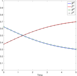
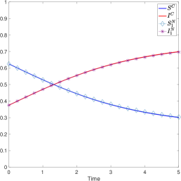
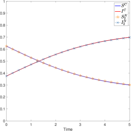
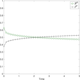
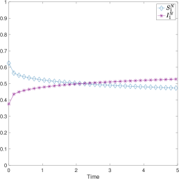
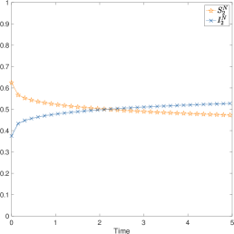
First of all we compare the exact fractional solutions (1.5)-(1.6) and the two numerical solutions (4.10)-(4.11) and (4.12)-(4.13) for α=0.99𝛼0.99\alpha=0.99, which approximately corresponds to the classical derivative. Note that we do not use α1𝛼1\alpha\equiv 1 since the second numerical scheme works for α(0,1)𝛼01\alpha\in(0,1), as already observed in Remark 4.2. In Figure 1 we show the results. As expected, the exact fractional solution and the two numerical solutions to (1.1) overlap the solution for α=1𝛼1\alpha=1.

Refer to caption
(a)
Refer to caption
(b)
Refer to caption
(c)
Figure 1: Comparison between the solutions to the SIS model and the explicit and numerical fractional solutions to (1.1) with α=0.99𝛼0.99\alpha=0.99. The analysis shows correspondence between SIS model and the case α=1𝛼1\alpha=1 of our model. This result was expected and it confirms the continuity wit respect to α𝛼\alpha (see (P4)).

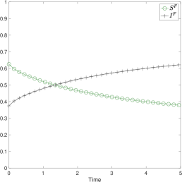
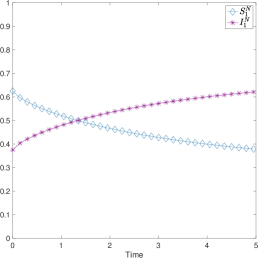
In Figures 2 and 3 we show the results obtained with α=0.7𝛼0.7\alpha=0.7 and α=0.3𝛼0.3\alpha=0.3. In the first case the two density curves are closer each other and the intersection point between them slightly moves to the right with respect to the solution shown in Figure 1. Such behavior is further emphasized by lower values of α𝛼\alpha, as shown for example in Figure 3. Note that, in both cases the three methodologies produces almost identical results.
Refer to caption
(a)
Refer to caption
(b)
Refer to caption
(c)
Figure 2: Comparison between the explicit and numerical fractional solutions to (1.1) with α=0.7𝛼0.7\alpha=0.7.
Refer to caption
(a)
Refer to caption
(b)
Refer to caption
(c)
Figure 3: Comparison between the explicit and numerical fractional solutions to (1.1) with α=0.3𝛼0.3\alpha=0.3.

To further investigate on the three methodologies, we compute the Lsuperscript𝐿L^{\infty}-norm of the difference between the exact fractional solutions (1.5)-(1.6) and the two numerical solutions (4.10)-(4.11) and (4.12)-(4.13) and between the two numerical solutions each others, as shown in Table 1. We observe that the errors range from orders of 105superscript10510^{-5} to 103superscript10310^{-3}, increasing with respect to the decrease of α𝛼\alpha. This fact further certifies the similarity between the three proposed methodologies.

α𝛼\alpha IFI1Nsubscriptdelimited-∥∥superscript𝐼𝐹subscriptsuperscript𝐼𝑁1\left\lVert\mathnormal{I}^{F}-\mathnormal{I}^{N}_{1}\right\rVert_{\infty} IFI2Nsubscriptdelimited-∥∥superscript𝐼𝐹subscriptsuperscript𝐼𝑁2\left\lVert\mathnormal{I}^{F}-\mathnormal{I}^{N}_{2}\right\rVert_{\infty} I1NI2Nsubscriptdelimited-∥∥subscriptsuperscript𝐼𝑁1subscriptsuperscript𝐼𝑁2\left\lVert\mathnormal{I}^{N}_{1}-\mathnormal{I}^{N}_{2}\right\rVert_{\infty}
0.99 1e–05 9e–04 9e–04
0.7 1e–05 2e–03 2e–04
0.3 3e–05 8e–03 8e–03
Table 1: Comparison of the Lsuperscript𝐿L^{\infty}-norm between the solutions computed with the three methodologies for different values of α𝛼\alpha.

4.2.2 Test with c=0𝑐0c=0

We focus now on the case of carrying capacity c=0𝑐0c=0. We fix this set of parameters: β=0.7𝛽0.7\beta=0.7, γ=0.07𝛾0.07\gamma=0.07, μ=0.63𝜇0.63\mu=0.63, σ=1𝜎1\sigma=1 and c=0𝑐0c=0. Moreover, the initial data are I(0)=1/(2β)𝐼012𝛽\mathnormal{I}(0)=1/(2\beta) and S(0)=1I(0)𝑆01𝐼0\mathnormal{S}(0)=1-\mathnormal{I}(0), the final time is T=1𝑇1T=1 and the time step Δt=0.01Δ𝑡0.01\Delta t=0.01.

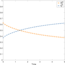
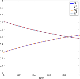
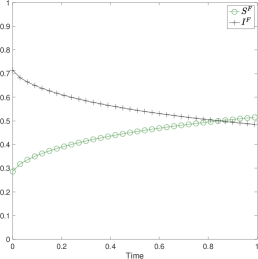
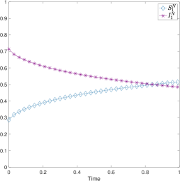
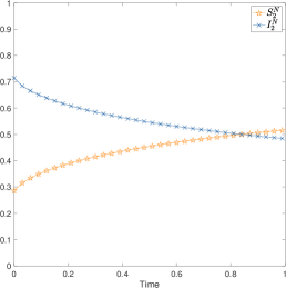
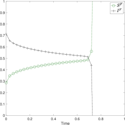
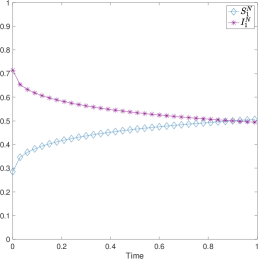
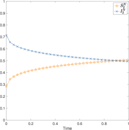
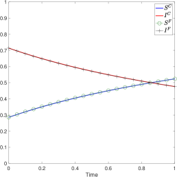
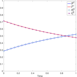
In Figure 4 we compare the exact fractional solutions (1.8)-(1.9) and the two numerical solutions (4.10)-(4.11) and (4.12)-(4.13) for α=0.99𝛼0.99\alpha=0.99. Again, we observe that the fractional solutions, both explicit and numerical, perfectly overlap the solution to the SIS model. In Figure 5 we show the results obtained with α=0.7𝛼0.7\alpha=0.7. Analogously to the example with c0𝑐0c\neq 0, the point of intersection between the two densities of population slightly moves to the right with respect to the solution shown in Figure 4. Moreover, the three different methodologies produce again almost identical results. Finally, in Figure 6 we show the results obtained with α=0.5𝛼0.5\alpha=0.5. In this case, the explicit fractional solutions (1.8)-(1.9) blow up in finite time, since the final time T𝑇T is greater than the radius of convergence, while the two numerical solutions show that the intersection point between the two curves further moves to the right with respect to Figure 5.
Refer to caption
(a)
Refer to caption
(b)
Refer to caption
(c)
Figure 4: Comparison between the solutions to the SIS model and the fractional solutions to (1.1) with α=0.99𝛼0.99\alpha=0.99 (continuity w.r. to α𝛼\alpha).
Refer to caption
(a)
Refer to caption
(b)
Refer to caption
(c)
Figure 5: Comparison between the fractional solutions to (1.1) with α=0.7𝛼0.7\alpha=0.7.
Refer to caption
(a)
Refer to caption
(b)
Refer to caption
(c)
Figure 6: Comparison between the fractional solutions to (1.1) with α=0.5𝛼0.5\alpha=0.5.

Conclusions

In this work we have studied the fractional SIS model with constant population size. We have proposed an explicit representation of the solution to the fractional model under particular assumptions on parameters and initial data. By considering the basic reproduction number we rearrange the SIS model and obtain a logistic equation. In the new formulation of the problem the carrying capacity has a new meaning based on the parameters of the SIS model. We exploit such a formulation in order to study the fractional SIS model and obtain a fruitful characterization of the problem, despite of many difficulties introduced by non-locality. In our formulation the carrying capacity can equal zero and this brings our attention to a different non-linear problem which in turns, it is related to the underlined SIS model. We have introduced two different numerical schemes to approximate the model and perform numerical simulations, with which we have tested the proposed explicit solution.

References

  • [1] E. Ahmed, A. El-Sayed, A. El-Mesiry, H. El-Saka, et al., Numerical solution for the fractional replicator equation, Int. J. Mod. Phys. C, 16 (2005), pp. 1017–1026.
  • [2] R. M. Anderson and R. M. May, The population dynamics of microparasites and their invertebrate hosts, Philos. T. R. Soc. B, 291 (1981), pp. 451–524.
  • [3] I. Area, J. Losada, and J. J. Nieto, A note on the fractional logistic equation, Physica A, 444 (2016), pp. 182–187.
  • [4] K. Diethelm, The Analysis of Fractional Differential Equations, Springer-Verlag Berlin Heidelberg, 2010.
  • [5] K. Diethelm and A. D. Freed, The FracPECE Subroutine for the Numerical Solution of Differential Equations of Fractional Order, Forschung und wissenschaftliches Rechnen, 1999 (1998), pp. 57–71.
  • [6] M. D’Ovidio and P. Loreti, Solutions of fractional logistic equations by Euler’s numbers, Physica A, 506 (2018), pp. 1081–1092.
  • [7] A. El-Sayed, A. El-Mesiry, and H. El-Saka, On the fractional-order logistic equation, Applied Mathematics Letters, 20 (2007), pp. 817–823.
  • [8] F. Ferrari, Weyl and Marchaud Derivatives: A Forgotten History, Mathematics, 6 (2018), p. 6.
  • [9] Y. Giga, Q. Liu, and H. Mitake, On a discrete scheme for time fractional fully nonlinear evolution equations, Asymptot. Anal., (2019), pp. 1–12.
  • [10] H. W. Hethcote, Three basic epidemiological models, in Applied mathematical ecology (Trieste, 1986), vol. 18 of Biomathematics, Springer, Berlin, 1989, pp. 119–144.
  • [11] W. O. Kermack and A. G. McKendrick, A contribution to the mathematical theory of epidemics, P. Roy. Soc. A-Math. Phy., 115 (1927), pp. 700–721.
  • [12] S. Pooseh, H. S. Rodrigues, and D. F. Torres, Fractional derivatives in dengue epidemics, in AIP Conf. Proc., vol. 1389, 2011, pp. 739–742.
  • [13] A. Quarteroni, R. Sacco, and F. Saleri, Numerical mathematics, vol. 37 of Texts in Applied Mathematics, Springer-Verlag, Berlin, second ed., 2007.
  • [14] A. F. Rositch, J. Koshiol, M. G. Hudgens, H. Razzaghi, D. M. Backes, J. M. Pimenta, E. L. Franco, C. Poole, and J. S. Smith, Patterns of persistent genital human papillomavirus infection among women worldwide: A literature review and meta-analysis, Int. J. Cancer, 133 (2013), pp. 1271–1285.
  • [15] P.-F. Verhulst, Notice sur la loi que la population suit dans son accroissement, Corresp. Math. Phys., 10 (1838), pp. 113–126.
  • [16] B. West, Exact solution to fractional logistic equation, Physica A, 429 (2015), pp. 103–108.
  • [17] X.-J. Yang and J. Tenreiro Machado, A new insight into complexity from the local fractional calculus view point: modelling growths of populations, Math. Mod. Meth. Appl. S., 40 (2017), pp. 6070–6075.
  • [18] F. W. Zhang and L. F. Nie, Dynamics of SIS epidemic model with varying total population and multivaccination control strategies, Stud. Appl. Math., 139 (2017), pp. 533–550.
  • [19] J. Zhou and H. W. Hethcote, Population size dependent incidence in models for diseases without immunity, J. Math. Biol., 32 (1994), pp. 809–834.