How Reliable are Test Numbers for Revealing the COVID-19 Ground Truth and Applying Interventions?

Abstract

The number of confirmed cases of COVID-19 is often used as a proxy for the actual number of ground truth COVID-19 infected cases in both public discourse and policy making. However, the number of confirmed cases depends on the testing policy, and it is important to understand how the number of positive cases obtained using different testing policies reveals the unknown ground truth. We develop an agent-based simulation framework in Python that can simulate various testing policies as well as interventions such as lockdown based on them. The interaction between the agents can take into account various communities and mobility patterns. A distinguishing feature of our framework is the presence of another ‘flu’-like illness with symptoms similar to COVID-19, that allows us to model the noise in selecting the pool of patients to be tested. We instantiate our model for the city of Bengaluru in India, using census data to distribute agents geographically, and traffic flow mobility data to model long-distance interactions and mixing. We use the simulation framework to compare the performance of three testing policies: Random Symptomatic Testing (RST), Contact Tracing (CT), and a new Location Based Testing policy (LBT). We observe that if a sufficient fraction of symptomatic patients come out for testing, then RST can capture the ground truth quite closely even with very few daily tests. However, CT consistently captures more positive cases. Interestingly, our new LBT, which is operationally less intensive than CT, gives performance that is comparable with CT. In another direction, we compare the efficacy of these three testing policies in enabling lockdown, and observe that CT flattens the ground truth curve maximally, followed closely by LBT, and significantly better than RST.

1 Introduction and Summary of Observations

Beginning March 11, fearing the quick spread of COVID-19, all schools were shut down in Bengaluru, India. Colleges, universities, and cinema halls were soon to follow and were shut down within a week. On Sunday March 22, the Prime Minister of India announced a country-wide “Janta curfew” for a day. Finally, on Tuesday, March 24, the Prime Minister announced a 21 day complete lockdown for the country, which has been extended till May 3rd now. It is interesting to note that there were just 6 confirmed cases and 1 death till March 15 across the state of Karnataka, to which Bengaluru belongs, when the mega-city of Bengaluru was shut down. In fact, till March 24 there were only 517 confirmed cases across India, a number which may appear small compared to the large ($\approx$ 1.3 Billion) population of the country. Even the growth rate of the number of cases was not very high. Yet, the policy makers decided to engage a lockdown, perhaps even with popular public support.

Clearly, the perceived number of ground truth cases and its increase rate must have been higher than the actual confirmed cases to facilitate such a drastic measure. But how well does the daily positive test outcome trend reflect the unknown ground truth? Can policy makers use it reliably to implement non-pharmaceutical interventions, such as lockdown, even when the number of daily tests is very low? Such questions become even more important in view of several media articles and expert opinions questioning if India is testing its residents enough [16, 17]. Given the large population of India, it is unlikely that we can scale the tests to the level of countries like Iceland, which has tested about 5% of its population. Thus, what one expects out of more testing is to get a better estimate of the ground truth trend to enable better preparedness and well-informed policy decision making. With this context in mind, we ask a basic question: How much testing is enough?

We undertake a systematic mathematical modeling and simulation-based study of a variety of testing policies, and compare their efficacy for enabling interventions such as lockdown. Based on our experiments, our main findings can be summarized as follows:

1. If a sufficient fraction of symptomatic population shows up for testing, then testing a small random sample of symptomatic patients can give a good idea of the ground truth trend.

2. Contact tracing (CT), where contacts of a COVID-19 patient are tested, returns a significantly higher number of positive test outcomes than the random symptomatic testing (RST) as above. More importantly, a decision for locking down the population based on CT can help reduce the peak ground truth number of cases (‘flatten the curve’) much better than RST.

3. By using a location- and mobility pattern-aware sampling, it is possible to get performance similar to that of CT using operationally less intensive testing procedures.

We present the precise observations and describe the setup later in the paper, but we quickly note here that we use the derivative of the ground truth curve as an indicator of the ground truth trend – indeed, visually it appears to be a good indicator. It is this indicator of ground truth trend that RST reveals well.

Our conclusions are based on agent-based simulation for a population of 100000 individuals or agents distributed across a realistic synthetic city, interacting based on a realistic mobility pattern. Specifically, we use publicly available census data to distribute the agents across the 198 (urban) wards in the city of Bengaluru. The agents have health states related to COVID-19 and another, generic, ‘flu’-like disease condition with similar symptoms, which evolve independently. A susceptible agent (in COVID state S) can get infect when it meets a COVID-19 infected agent (in COVID state I). The agents can interact with other agents in their neighbourhood or agents that visit similar locations daily. We instantiate the mobility of agents across the city using mobility data obtained from traffic flows.

This evolution model drives the unknown state, a part of which is observed by testing policies, stored in a separate module in our implementation. A testing policy determines which agents will be subjected to testing and applies a randomized test to the selected agent. The history of test results is stored and is made available to intervention policies, which are stored in yet another module. An intervention policy outputs a control action which modifies the state evolution dynamics. For instance, a lockdown intervention will disable the interaction between the agents. We assume that the borders of the city are closed and there is no interaction with the outside world.

Our overall simulation framework, made available as a Python package at [9], is flexible and can incorporate any new testing policy or intervention policy. Furthermore, the state evolution model can be easily modified to incorporate more “mixing points” such as buses, malls, etc.. In fact, our goal is to incorporate real-time mobility data obtained from digital platforms, as suggested in [8], to have an updated representation of mixing in the city.

A disclaimer: Our model has not been calibrated to match the actual number of cases in Bengaluru. Neither do our conclusions enjoy rigorous theoretical backing. These results are preliminary and are based on experiments with our simulation framework. They provide, we hope, insight into questions raised above and exhibit the utility of our simulation framework that can used for such studies. This is work in progress, released early to ensure timely dissemination.

There is large body of work using mathematical models and simulation to study spread of COVID-19 and facilitate decision making. A very timely publication was the report [7] from the COVID-19 response team of Imperial College, London, earlier versions of which raised an alarm about possible worst-case scenarios if COVID-19 is allowed to grow unchecked. This in turn is based on a long-line of work from the same group on mathematical modeling and simulation of epidemic spread; see, for instance, [6]. Our models of state evolution are similar to these works, but at this point are not as elaborate as these works. More refined models with comorbidity and age-dependent evolution have been considered in [18].

While distance based modeling of interaction of agents is quite popular, with footing in random graph theory, using real mobility and traffic data to model interaction of agents is also gaining prominence in epidemiological studies. In this paper, we have only considered traffic data obtained using surveys, somewhat similar to how data is obtained in [11]. A more effective method can be the prescription in [8] where location services and mobile phone usage data is used to obtain real-time daily mobility patterns. Looking ahead, we would like to integrate such data into our framework.

While most of prior work has treated the outcome of tests as the actual ground truth number of COVID-19 cases, very recently, articles [14] and [5] have appeared that explicitly study the role of the testing policy. The former has a similar setup as ours, except that the simulation is event-driven and uses a more detailed simulation of agent interaction. However, only contact tracing is considered and an ideal situation where there is no other flu with similar symptoms is assumed. In a way, this framework assumes that one can directly access the ground truth. The article [5] presents a similar discussion as our results, but the approach appears to be more statistical and not based on explicit epidemic modeling/simulation. We remark that our proposed new testing algorithm uses ideas from multi-armed bandit problems; the paper [4] proposes an algorithm that uses similar ideas towards achieving a good test allocation strategy.

The remainder of this paper is organized as follows. We present the details of our modeling and simulation framework in the next section. A comparison of the three testing policies we consider when there is no intervention is given in Section 3, and a comparison of their efficacy in enabling interventions in Section 4. We conclude with some discussion on policy implications and next steps in the final section.

2 Simulator Description and Features

2.1 Simulation model

We consider an agent based simulation framework to model the propagation of an epidemic in a city. In our general framework, a city is populated using $n$ agents distributed across fixed “localities” of a city in proportion to their population densities. Each agent $i$ represents a person with attributes such as location associated with it. The health of an agent is captured by its “COVID State” $C_{i}(t)$ on day $t$. A distinguishing feature of our setup is an additional “Flu State” $F_{i}(t)$ which represents the presence of another flu with similar symptoms as COVID-19. This allows us to model the erroneous prescription of COVID-19 test to a person who shows similar symptoms due to presence of another flu, which we believe is essential for a realistic modeling of testing.

The evolution of $C_{i}(t)$ is determined by two factors: a local evolution model for each agent’s state and evolution due to interaction between agents. For local evolution, we use the popular SEIR model for $C_{i}(t)$ where the COVID state of an agent can take values in the set $\{S,E,I,R\}$ representing, respectively, susceptible (S), exposed (E), infected (I), and recovered (R) conditions. Note that this model is a simplification of the dynamics used in [7] and combines the several stages such as hospitalization and death into a single state R. The origin of such models in epidemiology can be traced back to the pioneering work of Kermack and McKendrick in 1920s, and they have been used for modeling COVID-19 dynamics in [8, 12, 18, 14] The collective states $C(t)=\{C_{i}(t),1\leq i\leq n\}$, $1\leq t\leq T$, form a discrete-time Markov chain where $C_{i}(t)$ on day $t$ changes to the state $C_{i}(t+1)$ on day $t+1$ according to a pre-specified probability transition matrix $T$ depicted in Figure 1.

Figure 1: COVID state evolution of each agent.

Specifically, each agent changes its state from E to I to R independently of all the other agents. The transition probabilities in Figure 1 are set to parameters $1/T_{ss^{\prime}}$ where $T$ is the average transition time between states $s$ and $s^{\prime}$. Although the values chosen for our simulations are only approximations, such average times have been studied and reported extensively in literature, and the most up-to-date estimates can be used in the model by the interested practitioner.

Note that an agent makes a transition from S to E based on its interaction with other agents. When an agent in state $I$ meets another agent in state $S$, the latter agent gets infected with a pre-specified probability $p$. To model the meeting of agents, we include two components: The first is a “neighbourhood” component where each agent meets a set of randomly chosen agents from the same neighbourhood. In addition, each agent meets a fixed set of agents from its neighbourhood, generated randomly at start and then fixed throughout the simulation. Note that, for an agent, its neighbourhood need not coincide with its locality and can include a set of close-by localities. In our simulation, we have defined a neighbourhood as a set of localities touching (geographically) a given locality.

The second component represents interaction with agents from different localities, not necessarily the neighbouring ones. Here we propose to use data about mobility in the city. Here, too, an agent visiting a location on a day interacts with a set of randomly chosen agents generated afresh everyday as well as fixed set of agents set upfront.

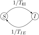
One final component of our model is the evolution of Flu state $F_{i}(t)$. We remark that the inclusion of this state is only to model the noise in applying a testing policy. Thus, we use a simple, intrinsic, SI model for $F_{i}(t)$ where it is evolves as a Markov chain independently for each $i$ and taking values in $\{S,I\}$ with transition probabilities depicted in Figure 2. Note that an important distinction between the COVID and Flu models is that in the former the process “terminates” once the state $R$ is reached since we assume that a person who has been infected with COVID-19 once cannot be infected again. However, a person keeps on shifting from $S$ to $I$ Flu states indefinitely – this is because the ”Flu state” is an proxy for the individual contracting any illness with similar symptoms as COVID-19. As we shall elaborate later, any testing policy that makes a pool of symptomatic patients will treat an agent with $C_{i}(t)=I$ and $F_{i}(t)=I$ identically (if all their other features such as locality match).

Figure 2: Flu state evolution of each agent.

This template for an interaction model is very generic and can incorporate various movements across the city in form of origin-destination flow data. Even bus routes can be included by considering them as locations. However, we have only implemented a restricted form of this interaction in the first version of our simulator used for experiments in this paper. Specifically, the number of fixed and randomly selected agents met in the neighbourhood and the locality visited are fixed to be the same for all the agents. Furthermore, only one visited location is set per agent, as a part of its feature matrix. However, we remark that it is easy to extend our model to include multiple locations (such as workplace, bus-used, etc.).

Before specifying the parameters used for the results of this paper in the next section, we remark that our framework requires mobility data to be fed in form of an origin-destination (OD) matrix. Such a matrix has number of rows $N_{r}$ as the number of localities and the number of columns $N_{c}$ representing the locality or community visited daily. The $(i,j)$-th entry of this matrix represents the probability with which a person from locality $i$ goes to locality $j$, whereby the $i$th row constitutes a probability vector that sums to one. We use this vector to generate the locality visited by each agent in locality $i$, independently of other agents. Note that we can have multiple such OD matrices, one for each community, and each person can be a member of one community each for every matrix available in the model. In its current form, our implementation allows the membership to depend only on the location of the agents. Furthermore, agents have not been endowed with other potentially relevant features such as age and comorbidity which determine COVID state evolution in practice. We plan to include these enhancements in a subsequent version.

We close this section by noting that the state evolution of our model is defined in the file evolution.py of our implementation. Also, we point out that the state of the city is captured by a pandas data frame City Population, abbreviated as CP, with $N$ rows and columns corresponding to various features of each agent.

A caution: Our implementation is designed to use multiple CPU cores in parallel, but the specific dynamics change when number of cores are increased. In particular, increasing the number of cores used changes the number of state transitions happening in parallel, reducing the overall growth rate. Throughout this paper, we have set the number of cores to 8.

2.2 Parameters used for simulation

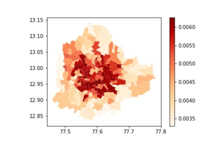
In this paper, we instantiate the general framework described above for the city of Bengaluru in India. For simplicity, we only consider an SIR model for COVID state where the E state is skipped by setting $T_{EI}=1$. We consider the 198 urban wards of Bengaluru that come under the city municipal corporation (Bruhat Bengaluru Mahanagara Palike, BBMP) and use the census data (converted to a .geojson file using data from [2, 3]) to populate $N=100000$ agents across the city; see Figure 3 for depiction of population densities.

Figure 3: Ward-wise population density of Bengaluru.

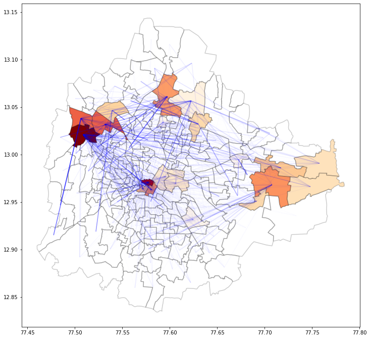
For modeling mobility across the city, we use data on vehicle mobility across Bengaluru acquired from the Centre for Infrastructure, Sustainable Transportation and Urban Planning (CiSTUP), Indian Institute of Science, Bangalore. This is similar in spirit to the prescription in [8], but instead of dynamic digital data, we use static data obtained using surveys similar to [11, 12]. This data includes OD matrices for vehicles of different categories across Bengaluru which was obtained by conducting household surveys across the city. We have only used the data for car traffic in our interaction model. Furthermore, it includes daily bus ticket sales obtained from BBMP; however, in this paper, we have not used the bus ticket sales data. To reduce computational load, we restrict the OD matrix to the 20 destination locations seeing the highest inflow, depicted in Figure 4. Note that we also have a fictitious destination 21 representing an agent not visiting any of these 20 destination.

Figure 4: The top 20 wards with highest car traffic inflow in Bengaluru. The red component in the colour of each ward is proportional to the fraction of inflow traffic for the ward and the opaqueness of blue lines indicate the flow between the wards it joins.

With the interaction model set, we now list the values set for various parameters of our model described in the previous section:

Parameter	Value
COVID infection rate $p$	0.1
Average time from E to I for COVID state $T_{EI}$	1
Average time from I to R for COVID state $T_{IR}$	8
Average time from S to I for Flu state $T_{SI}$	50
Average time from I to S for Flu state $T_{IS}$	8
Number of randomly selected people each person meets in its neighbourhood	1
Number of fixed people each person meets in its neighbourhood	5
Number of randomly selected people each person meets at its workplace locality	2
Number of fixed people each person meets at its workplace locality	10

We remark that while our focus in this paper is not on careful calibration of the model, we have used reasonable parameter values based on results in [10, 13]. We execute each simulation for $1,00,000$ people for a duration of $T=100$ days. We mention in passing that we can easily incorporate bus data as well as movement data collected from location traces as suggested by [8] in our framework; we will do this in subsequent versions of our implementation.

2.3 The testing policy framework

A strength of our framework is its ability to incorporate testing policies. Our simulator takes as input a function testingPolicy described in the file tests.py. The history of testing of entire population is stored in an $(N\times T)$ matrix TestingHistory, which stores $0$ as the default value for each entry and updates the $(i,t)$-th entry to $1$ or $-1$, respectively, if agent $i$ is tested on day $t$ and the outcome is positive or negative.

We can admit any testing policy that selects a pool of candidates to be tested and applies the a common test function ${\tt test()}$ to each individual in the pool.The test function is defined to have $0$ probability of a false positive (this is in line with observed characteristics of the RT-PCR test for COVID-19 [19]), but a nonzero probability of false negative can be set. For simplicity, we have set the probability of false negative to $0$ in our simulations.

In selecting the pool of candidates, a testing policy can only use observable features such as locality of individual, the workplace visited, and whether an agent is symptomatic. Note that a symptomatic agent can have either Flu state I or COVID state I, but a testing policy (obviously so) cannot use the actual COVID or Flu state of a person.

We have implemented and simulated three testing policies. Each policy selects a fixed number $N_{\tt test}$ of symptomatic agents at each time step (day) to apply tests. The following policies are simulated:

1. Random Symptomatic Testing (RST): The daily pool of agents to be tested is selected randomly (from among people who are symptomatic).

2. Contact Tracing (CT): The daily pool is selected randomly from the set of all symptomatic among the neighbourhood contacts and the workplace contacts of all the patients. If this set is of smaller cardinality than $N_{\tt test}$, which happens often, we enhance it with symptomatic from across locations.

3. Location Based Testing (LBT): This policy is a bit involved and will be described in detail in Section 3. At a high level, this policy gives priority for testing to symptomatic agents belonging to localities and workplaces with higher infection.

A few remarks are in order. First, these policies are enabled by maintaining a list of fixed contacts in the neighbourhood and the workplace, which can be identified for CT. We assume that the randomly selected daily contacts that an agent interacts with cannot be traced, as is the situation in practice.

Second, we mention that CT is an “infra-heavy” testing policy requiring operational support to trace contacts and test them. In contrast, RST and LBT are algorithms that do not require operational support but require a careful design of policy mechanisms to ensure prescribed sampling.

Finally, we briefly outline the connection between testing policies in practice and the ones we have implemented in our simulation framework. All the testing policies described above start with a list of symptomatic agents. In practice, such a list emerges when symptomatic patients reach out to their medical provider. An effective information campaign by the government can ensure that patients with symptoms matching those seen in COVID-19 come out for testing. Nonetheless, the exact percentage of symptomatic patients that come out can vary with localities, since each locality differs in income levels and availability of medical facilities. To model this, we incorporate “under-reporting” in our framework which can be represented by a locality wise reporting probability vector. Further, our tests sample randomly from the pool of symptomatic patients. In practice, this sampling is implemented by medical professionals who recommend a subset of symptomatic patients for testing. We believe that all the policies we have simulated can be (and, for some, have been) converted to an implementable form on the ground at least in the Indian context, e.g., the containment plan of the Ministry of Health and Family Welfare, Govt. of India, already lays down “hotspot detection’ as part of a testing/intervention strategy [15].

2.4 The interventions framework

Our framework can simulate evolution under interventions. A policy intervention such as a city-wide lockdown is implemented as modifying the interactions between different agents in the simulation. The intervention policy is specified as an input in the form of Python function interventionPolicy which is accessed everyday (for every iteration) to produce a list of interventions. When updating the state of each agent (using the function updateState specified in evolution.py), the list of interventions enabled on each day is used to decide which interactions will be allowed for the agent. This is done by making access to the function InterventionRule, which interprets the impact of intervention for state evolution. In particular, we have implemented and simulated the following three interventions available as respectively as Python functions InterventionQuarantine, InterventionLockdown, and InterventionLockdownFixed specified in interventions.py:

1. Quarantine: Each agent that is tested positive for COVID-19 on day $t$, along with all the agents on its list of neighbourhood and workplace contacts, are placed on quarantine for a period of 10 days starting from day $t+1$. Namely, the agent is not allowed to interact with any other agent during this quarantine period.

2. Indefinite lockdown: All agents are not allowed to interact with any other agent once a particular trend is detected in the positive test count.

3. Fixed duration lockdown: All agents are not allowed to interact with any other agent for a fixed period of time once a particular trend is detected in the positive test count.

In the last two lockdowns, the rule to start a lockdown has not explicitly been mentioned. We will elaborate on this later, but roughly, a lockdown is triggered once the slope of positive COVID-19 tests crosses a threshold. Thus, the efficacy of an intervention policy is tied intrinsically to the testing policy used. As such the intervention policy function is given access to the overall population state CP, the history of interventions imposed, and the testing history matrix. If an additional state is required for implementing a policy – such as quarantine requires us to store the quarantine state of each agent – it is included as a part of CP.

In summary, our simulation framework separates state evolution functions (in evolution.py), testing policy (in tests.py), and intervention policy (in interventions.py). A new test or a new intervention can easily be incorporated by maintaining the input-output structure.

3 Testing Strategies and Performance Comparison

This section details the testing strategies that we have explored using the simulation framework of Section 2, and compares their performance. For this section, no intervention is performed based on the test outcomes. The impact of tying interventions to test outcomes is discussed in Section 4.

3.1 Testing strategies

At a high level, a test strategy is expressed as a test selection rule, applied in each time step (day) of the simulation, that maps the current population, together with the past testing history, to a subset of individuals that are subsequently tested for COVID-19 infection. This map cannot depend on the actual health states of the individuals (e.g., their COVID state), but can rely on only their observable attributes, such as whether they display symptoms of illness or whether they reside in a specific ward or wards. The map can also be randomized to reflect random sampling from certain locations without necessarily relying on the onset of symptoms. The general pseudocode of a test selection rule appears in Algorithm 1.

All individuals selected by a test selection rule are assumed to undergo medical testing (e.g., RT-PCR testing) represented by the individual test subroutine Algorithm 2 (defined as the function test in tests.py), which models false negatives arising in the testing process at an assumed rate $r\in[0,1]$.

In the sequel, the testing strategies we describe are specifications of test selection rules, assuming access to a standard individual testing subroutine.

input : Current day $t$, Past testing history $\mathcal{H}_{t-1}$ , i.e., individuals tested on day $s\leq t-1$ and their test results, Observable attributes of all individuals on day $t$

output : Set of individuals to be tested on day $t$

$S=\emptyset$ ;

  // holds set of individuals to be tested

for individual in population do

       if condition is satisfied then

             add individual to $S$ ;

       end if

      

end for

return $S$

Algorithm 1 Test selection algorithm (general)

input : Individual $i$, False negative rate $r$

output : Result $\in\{+1,-1\}$

Result $\leftarrow-1$;

if $i$’s CovidState is “I” then

       Result $\leftarrow+1$ with probability $(1-r)$

end if

return Result

Algorithm 2 TestIndividual (Individual test subroutine)

3.1.1 Random Symptomatic Testing

The first, and simplest, testing strategy we consider is Random Symptomatic Testing (RST). This strategy (pseudocode in Algorithm 3) looks at the pool of people who display symptoms typical of the disease, and randomly samples as many of them as possible to fill up a predefined budget. This is considered a baseline testing strategy under budget constraints in the experiments reported here.

input : Test budget $b$, Current day $t$, Past testing history $\mathcal{H}_{t-1}$ , i.e., individuals tested on day $s\leq t-1$ and their test results, Observable attributes of all individuals on day $t$

output : Set of individuals to be tested on day $t$

$A\leftarrow$ Individuals displaying symptoms on day $t$ ;

$S\leftarrow$ Random subset of $\min(b,|A|)$ individuals, sampled from $A$ without replacement ;

return $S$

Algorithm 3 Random Symptomatic Testing (RST) test selection algorithm

3.1.2 Contact Tracing

Contact Tracing (CT) is a testing strategy in which symptomatic contacts of individuals that have tested positive in the recent past are tested at the highest priority. If any more tests are available, then as many (randomly chosen) individuals as possible that are presently exhibiting symptoms are chosen for testing. Pseudocode for the CT test selection strategy appears in Algorithm 4. Note that in practice even the nonsymptomatic contacts are often tested, which is what should be done in a simulation with the SEIR model. But since we have disabled the ‘E’ (exposed) state for simplicity, we only test symptomatic contacts.

input : Test budget $b$, Current day $t$, Past testing history $\mathcal{H}_{t-1}$ , i.e., individuals tested on day $s\leq t-1$ and their test results, Observable attributes of all individuals on day $t$

output : Set of individuals to be tested on day $t$

$A\leftarrow$ Individuals displaying symptoms on day $t$ ;

$C\leftarrow$ All (fixed) symptomatic contacts of individuals tested +ve in the past 2 days (day-1 & day-2)

if $|C|<b$ then ;

 // more tests available than # traced contacts

       $S\leftarrow C\cup\left\{\min\{b-|C|,|A|\}\text{ individuals sampled from $A$ without replacement}\right\}$

else ;

 // fewer tests than # traced contacts

       $S\leftarrow\left\{b\text{ individuals sampled from $C$ without replacement}\right\}$

end if

return $S$

Algorithm 4 Contact Tracing (CT) test selection algorithm

3.1.3 Location-Based Testing

Location-Based Testing (LBT) is a testing rule that is designed to favour individuals who are ‘close’ to the currently known footprint of the COVID-19 infection. Closeness here is assumed to be high if (a) the individual’s locality contains many individuals known to have tested +ve in the past, or (b) many individuals who have tested +ve in the past are associated with the individual’s visit place.

The LBT selection rule (Algorithm 5) essentially computes a closeness or risk score of each person who reports symptoms, and prioritises individuals for testing depending on their risk scores. The risk score of a person can be thought of as a crude proxy for the posterior probability of that person being infected with COVID-19 on a given day, given all the observed history of tests.

For our implementation, we define the score of an individual $i$ on day $t$ as a weighted sum of the scores of its residence locality and its visit place. The score of a locality is an exponentially weighted average of the number of +ve tested individuals associated to it in the past, e.g., an individual who tested positive from the locality $\Delta$ days ago contributes $\alpha_{\text{loc}}(1+\epsilon)^{\Delta-1}$ to that locality’s score where $\alpha_{\text{loc}}>0$ is an adjustable parameter. The score of a visiting place is defined analogously. Pseudocode for the LBT selection algorithm appears in Algorithms 5 and 6.

input : Test budget $b$, Current day $t$, Past testing history $\mathcal{H}_{t-1}$ , i.e., individuals tested on day $s\leq t-1$ and their test results, Observable attributes of all individuals on day $t$

output : Set of individuals to be tested on day $t$

$A\leftarrow$ Individuals displaying symptoms on day $t$ ;

for Person in $A$ do

       Score[$i$] $\leftarrow$ getScore($i$, $t$)

end for

$S\leftarrow$ Random subset of $\min(b,|A|)$ individuals from $|A|$, successively sampled without replacement according to their Score

return $S$

Algorithm 5 Location-Based Testing (LBT) test selection algorithm

input : Individual $i$, Day $t$

output : (Risk) Score of $i$

parameters : $\alpha_{\text{loc}}$ (weight for locality per +ve case), $\alpha_{\text{vis}}$ (weight for visit place per +ve case), $\beta$ (relative weight of locality w.r.t. visit place), $\epsilon$ (amplification factor)

$v\leftarrow$ Visiting place which $i$ visits ;

$\ell\leftarrow$ Locality where $i$ resides ;

Score_$v$ $\leftarrow 0$ ;

Score_$\ell$ $\leftarrow 0$ ;

for $\tau$ in $1:(t-1)$ do

       Score_$v$ $\leftarrow$ $(1+\epsilon)$Score_$v$ + $\alpha_{\text{loc}}\left|\left\{j:j\text{ tested +ve on day $\tau$ \& $j$ visits $v$}\right\}\right|$ ;

       Score_$\ell$ $\leftarrow$ $(1+\epsilon)$Score_$\ell$ + $\alpha_{\text{vis}}\left|\left\{j:j\text{ tested +ve on day $\tau$ \& $j$ resides in $\ell$}\right\}\right|$

end for

return Score_$v$ + $\beta$ Score_$\ell$

Algorithm 6 getScore subroutine

Remark. We have not modelled the fact that both the conduct of tests and their reporting can suffer delays. For the interested experimenter, this can be incorporated easily by having the result of the TestIndividual subroutine (Algorithm 2) available to the parent test selection routine after a suitable delay.

3.2 Numerical Results and Discussion

We present and contrast here the numerical performance of the 3 testing strategies described previously – Random Symptomatic Testing (RST), Contact Tracing (CT) and Location-Based Testing (LBT). We run our experiments using the parameter settings of Section 2.2, without any nontrivial interventions enabled for individuals who test positive for COVID-19.

3.2.1 Test Performance with Clustered Seeding

Clustered seeding simulates the initial condition where all the initial COVID-19 cases are spatially localized. In our experiments, we initialize 50 COVID-19-infected individuals (out of a population of 100k) in a single locality (ward number 120, the ‘Cottonpete ward’) of the city of Bengaluru and let the outbreak evolve from there.

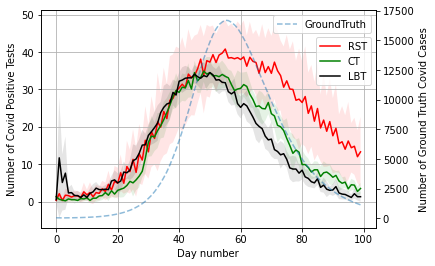
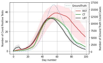
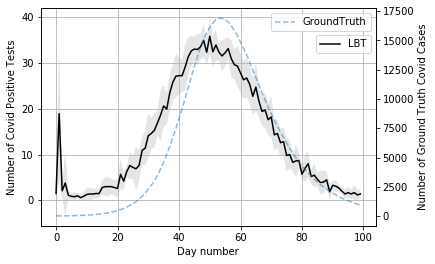
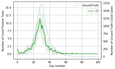
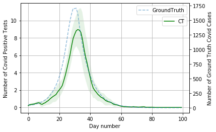
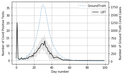
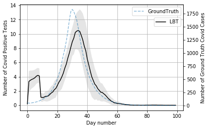
Figure 5 depicts the mean daily test score (number of tests with positive results) evolution with time for 10 independent simulation runs, along with the corresponding 1-standard deviation ranges shaded in lighter colour, for a daily budget of 50 tests/day. The ground truth number of cases per day is also plotted in the background. It is interesting to note that (a) RST shows high variance in reporting compared to the more biased CT and LBT, (b) while all 3 tests are equally accurate in capturing the trend of the ground truth in the phase leading up to the peak of actual case count, their performance after the peak is reached is quite different – CT and LBT tend to fall earlier than RST. Also interesting is the short-lived peak in the curve for LBT early on – this is due to the test aggressively prioritising testing from the affected seed locality. A smoothed version of the test results, plotted alongside, shows that smoothing can make the outputs of CT and LBT capture the rise-fall trend of the ground truth in a better fashion. Note that we have chosen a smoothing window of 8 days since the average time from COVID state ’I’ to COVID state ’R’ in our model is 8 days. Presumably the gains due to smoothing can be attributed to this fact – a patient tested positive 8 days ago is likely to remain positive till the current day.

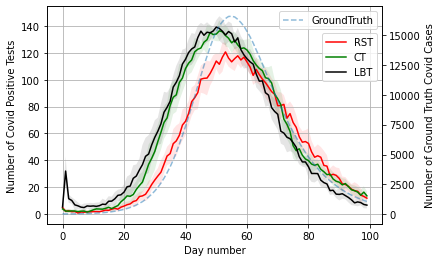
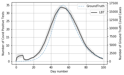
We also compare the tests with an enhanced (4x) budget of 200 tests/day (Figure 6). The extra budget appears to put to good use by the ‘smart’ tests CT and LBT, whose test numbers outstrip those of RST by a significant margin in the lead up to the peak. The faithfulness to the actual ground truth signal also appears to be much better for CT and RST here.

(a) Daily number of tests.

(b) Daily number of tests smoothened by taking an average over a window of 8 days.

Figure 5: Comparative test performance with clustered seeding and without intervention, for a time period of 100 days and with a testing budget of 50 tests/day. Results are averaged across 10 runs and error bars represent 1 standard deviation.

(a) Daily number of tests.

(b) Daily number of tests smoothened by taking an average over a window of 8 days.

Figure 6: Comparative test performance with clustered seeding and without intervention, for a time period of 100 days and with a testing budget of 200 tests/day. Results are averaged across 10 runs and error bars represent 1 standard deviation.

3.2.2 Test Performance with Uniform Seeding

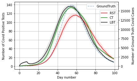
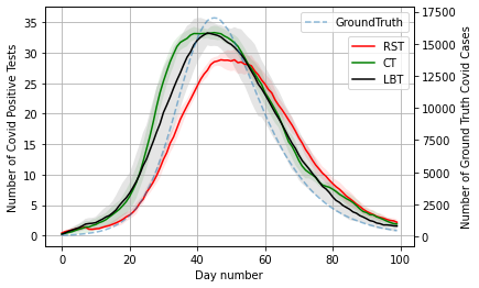
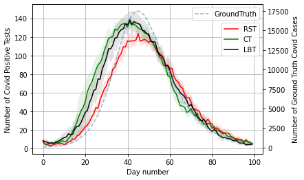
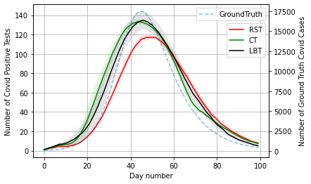
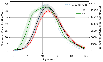
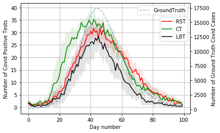
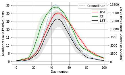
Figure 7 shows the results of applying the 3 tests with an initial seeding that is uniform across localities (city wards). Specifically, each of the (approx.) 200 localities in the simulation model hosts an independent Binomial$(5,0.1)$ number of COVID-19 infected seeds at start, resulting in about 100 seeds in the overall population (100k). Figure 8 plots the same metrics but for tests with an enhanced testing budget (200 per day).

The results show a clear advantage of the more advanced tests (CT, LBT) over the RST baseline, in the period leading up to the peak of ground truth COVID-19 cases. This potentially brings out the value of relying on predictive biased sampling (over and above the symptomatic sampling by RST) to detect a higher number of cases in the initial stages of the outbreak. We will see later (Section 4 ) that this confers a significant advantage in terms of timing when the results of the former tests are used to implement public (large-scale) lockdowns.

(a) Daily number of tests.

(b) Daily number of tests smoothened by taking an average over a window of 8 days.

Figure 7: Comparative test performance with uniform seeding and without intervention, for a time period of 100 days and with a testing budget of 50 tests/day. Results are averaged across 10 runs and error bars represent 1 standard deviation.

(a) Daily number of tests.

(b) Daily number of tests smoothened by taking an average over a window of 8 days.

Figure 8: Comparative test performance with uniform seeding and without intervention, for a time period of 100 days and with a testing budget of 200 tests/day. Results are averaged across 10 runs and error bars represent 1 standard deviation.

3.2.3 Test Performance with Under-reporting of Symptoms

We also examine what happens when individuals under-report symptoms when ill. This has the effect, in our simulation, of reducing the initial pool of symptomatic individuals which are input to the test selection strategy.

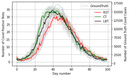
Uniform under-reporting. Figure 9 shows the test performance curves when each individual who is infected (either with COVID-19 or ”flu”) is assumed to report as symptomatic with probability $0.1$ independently (in the previous sections, this was assumed to occur with probability $1$). Though the 10x underreporting does not significantly affect the way in which all 3 tests capture the rise and fall in ground-truth cases, contact tracing emerges as the most informative detector of cases in the lead up to the peak.

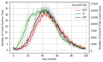
Non-uniform under-reporting. Figure 10 depicts the tests operating in a scenario where individuals report in a non-uniform manner whether they are symptomatic and hence to be considered for testing. Specifically, individuals from about $1/3$rd of the localities (wards) in the city (selected at random) report symptoms at rate 5% while the rest report at rate 100%. The initial seeding for COVID-19 cases is uniform across the localities as before. Contact tracing is seen to be robust to the rather skewed under-reporting enforced here, presumably due to its more accurate predictions of infection targets due to a richer local signal.

(a) Daily number of tests.

(b) Daily number of tests smoothened by taking an average over a window of 8 days.

Figure 9: Comparative test performance with uniform seeding and without intervention, for a time period of 100 days, a testing budget of 50 tests/day, and 10% reporting of symptoms. Results are averaged across 10 runs and error bars represent 1 standard deviation.

(a) Daily number of tests.

(b) Daily number of tests smoothened by taking an average over a window of 8 days.

Figure 10: Comparative test performance with uniform seeding and without intervention, for a time period of 100 days, a testing budget of 50 tests/day, and non-uniform reporting of symptoms. Results are averaged across 10 runs and error bars represent 1 standard deviation.

3.2.4 Estimating the Ground Truth number of Infections

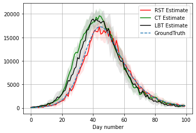
We explore the question of how well the test results, along with a record of the number of symptomatic individuals considered for testing, can be used to estimate the ground truth number of COVID-19 infections at any point in time. To this end, Figure 11 plots, for each day, an estimate of the ground truth computed as: the number of symptomatic patients $\times$ the error rate of the test, where the error rate of the test (on a day) is the ratio of the number of positive tests to the number of total tests performed. It is observed from the plot that the the (almost) unbiased RST algorithm gives the best fit to the ground truth evolution. The more aggressive (biased) CT and LBT strategies tend to overestimate the ground truth during the initial stages of the epidemic. We do not consider the problem of forming a more precise estimate using these strategies – it will require a precise knowledge of sampling probabilities and it is unclear if that will be available in practice.

Figure 11: Estimated no. of COVID-19 cases computed using numbers of symptomatic (at 100% reporting) and positive case counts. The simulation was carried out with uniform seeding and no intervention and a testing budget of 50 tests/day.

3.3 Visualization through Geo Plots

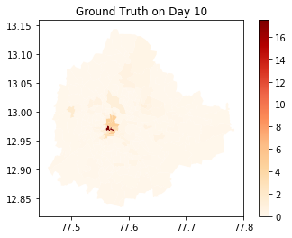
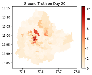
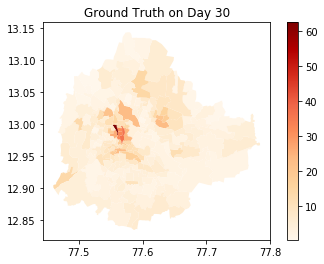
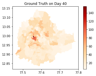
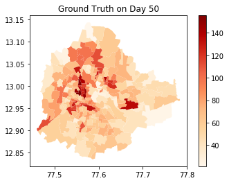
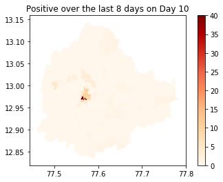
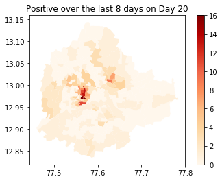
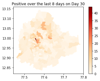
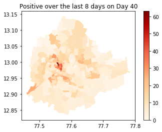
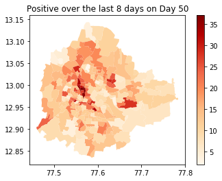
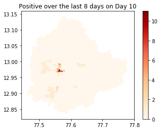
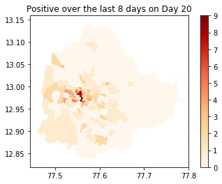
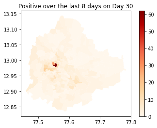
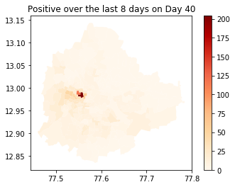
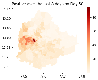
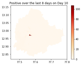
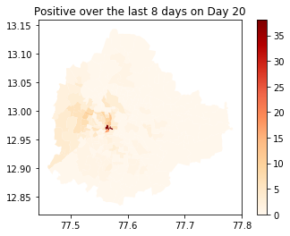
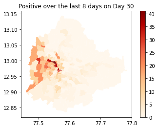
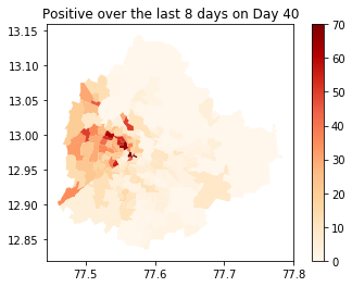
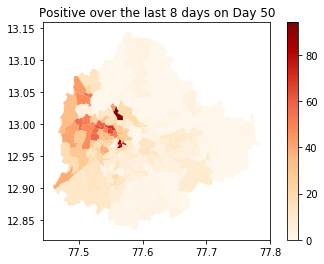
We depict an example spatio-temporal evolution of ground truth COVID-19 cases across the city, along with the corresponding positive cases detected in the recent past, in Figure 12. This illustrates the spatio-temporal nature of our simulation model and can be useful for making qualitative inferences about certain testing and/or intervention strategies. It can be noted that while all tests return a good signature of the source of infection initially, LBT yields vey high number of positive tests during the initial period, making it a suitable testing strategy for early detection and containment of the spread.

Figure 12: Geo plots illustrating the evolution of the ground truth and positive cases across the city and over time, with uniform seeding of COVID-19 cases. The X-axis represents time, with each successive column denoting an increment of 10 days from the previous column (or day $0$ for the first column). The first row represents the heat map for simulated ground truth COVID-19 cases by locality in Bengaluru. The second, third and fourth rows represent the heat maps for COVID-19 positive cases detected per locality by the Randomized Symptomatic Testing (RST), Contact Tracing (CT) and Location-based Testing (LBT) test selection algorithms, respectively, for the past 8 days.

4 Effect on Interventions

In this section, we compare the efficacy of our three testing policies in enabling interventions. As outlined earlier, an intervention policy takes into account the number of positive tests produced by the testing policy. An intervention such as lockdown is enabled once a particular trend is detected. Note that the purpose of such a lockdown is to “flatten the curve” by reducing the maximum number of daily COVID-19 cases in the ground truth. Such a reduction will reduce the stress on hospitals and other medical facilities.

We simulated COVID-19 evolution using the same rule for engaging an intervention policy using our testing polcies of RST, CT, and LBT. All the results we present in this section represent average over 10 runs of simulation; the mean behavior is depicted prominantly and the spread up to standard deviation is shown in a lighter color. Briefly, we find that CT outperforms RST significantly in reducing the maximum number daily of COVID-19 cases (in the ground truth). Interestingly, LBT performs comparably with CT – recall that the former is less operations-intensive that the latter. We present the three interventions we have considered in separate sections below.

4.1 Quarantine

We consider quarantine intervention where any person tested positive and all its contacts are placed under quarantine for 10 days. Note that this period of 10 days is shorted than the usual 14 to 21 days quarantine imposed in India; the reduction is to compensate for the absence of the E state in our simplified SIR model (average E to I period observed is 5 days). We have considered 50 tests (1 test per 2000 agents) per day starting with a clustered seeding where all the initial infections of COVID-19 are placed in one locality. Specifically, we place 50 agents in COVID state I in ward number 120 (the ‘Cottonpete ward’), as in the previous section. We present our results using RST, CT, and LBT in Figures 13, 14, and 15, respectively.

(a) Daily number of tests.

(b) Daily number of tests smoothened by taking an average over a window of 8 days.

Figure 13: Evolution of COVID-19 cases under quarantine intervention using RST.

(a) Daily number of tests.

(b) Daily number of tests smoothened by taking an average over a window of 8 days.

Figure 14: Evolution of COVID-19 cases under quarantine intervention using CT.

(a) Daily number of tests.

(b) Daily number of tests smoothened by taking an average over a window of 8 days.

Figure 15: Evolution of COVID-19 cases under quarantine intervention using LBT.

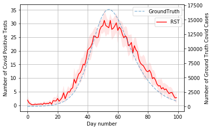
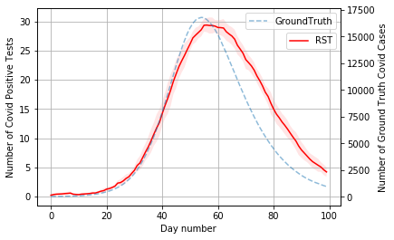
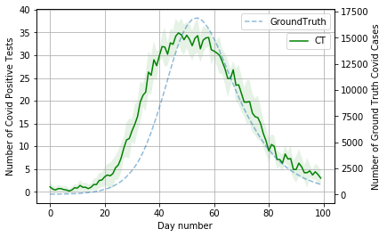
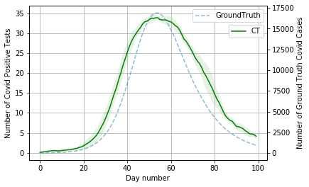
We observe that since the number of tests is very few, quarantine alone does not significantly reduce the maximum daily number COVID-19 cases (in the ground truth). Also, the number of positive tests that result using CT exceeds both RST and LBT, while RST captures the derivative of the ground truth COVID-19 cases well. These observations are similar to those for the case when no intervention was done and can be attribued to the unbiasedness of RST estimates when all symptomatic patients come out for testing.

Remark 1.

Note that LBT gets high number of positive tests in the beginning. This phenomenon was seen for clustered seed in the previous section as well and can be attributed to the fact that LBT tests many symptomatic agents from the location where infection was initially seeded. Later, as the infection spreads across the city and LBT has captured a large fraction of the initial 50 cases in ward number 120, LBT starts performing comparably with CT. In fact, this observation will hold in all the other interventions as well. This feature of LBT can be exploited to enforce a local lockdown of ward number 120 early on, preventing the further spread of COVID-19. However, we do not consider this intervention in this paper and will visit it in follow-up work.

4.2 Indefinite lockdown

We have implemented a threshold-based lockdown policy which disables the interaction of the agents with each other once the slope of the number of positive tests graph crosses a threshold. Specifically, denoting by $P(t)$ the number of positive test outcomes, our policy computes the slope of the “10 day chord” of a smoothened version $\overline{P}(t):=\frac{1}{8}\sum_{i=0}^{7}P(t-i)$ of $P(t)$ given by

$$\theta(t)=\frac{\overline{P}(t)-\overline{P}(t-10)}{10};$$

and starts a lockdown once $\theta(t)$ crosses a fixed threshold $\tau=0.5$. The selection of slope of the smoothened graph of $P(t)$ as a feature to use is based on our empirical observation that this slope captures the slope of the ground truth COVID-19 cases graph well. We term this policy the thresholded smoothened slope policy for lockdown. We use the same clustered seed as in the previous section and present our results using RST, CT, and LBT in Figures 16, 17, and 18, respectively.

(a) Daily number of tests.

(b) Daily number of tests smoothened by taking an average over a window of 8 days.

Figure 16: Evolution of COVID-19 cases under the indefinite lockdown intervention using the thresholded smoothened slope policy.

(a) Daily number of tests.

(b) Daily number of tests smoothened by taking an average over a window of 8 days.

Figure 17: Evolution of COVID-19 cases under the indefinite lockdown intervention using the thresholded smoothened slope policy.

(a) Daily number of tests.

(b) Daily number of tests smoothened by taking an average over a window of 8 days.

Figure 18: Evolution of COVID-19 cases under the indefinite lockdown intervention using the thresholded smoothened slope policy.

Looking at the ground truth number of cases under three testing policies, we observe that CT reduces the maximum daily COVID-19 cases the most by about 90% of the peak value in absence of any intervention. Even RST offers a significant reduction, by about 80%, but is much worse than CT. Remarkably, LBT, too offers very similar reduction as CT while requiring much less operational effort.

4.3 Fixed duration lockdown

The last intervention we consider is a fixed duration lockdown which, too, uses the thresholded smoothened slope policy to engage a lockdown. But after a lockdown is initiated, it is lifted after 14 days. We use the same clustered seed as in the previous sections and present our results using RST, CT, and LBT in Figures 19, 20, and 21, respectively.

(a) Daily number of tests.

(b) Daily number of tests smoothened by taking an average over a window of 8 days.

Figure 19: Evolution of COVID-19 cases under the fixed duration lockdown intervention using the thresholded smoothened slope policy.

(a) Daily number of tests.

(b) Daily number of tests smoothened by taking an average over a window of 8 days.

Figure 20: Evolution of COVID-19 cases under the fixed duration lockdown intervention using the thresholded smoothened slope policy.

(a) Daily number of tests.

(b) Daily number of tests smoothened by taking an average over a window of 8 days.

Figure 21: Evolution of COVID-19 cases under the fixed duration lockdown intervention using the thresholded smoothened slope policy.

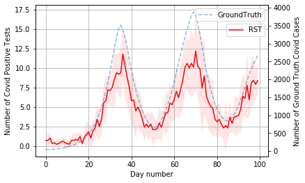
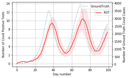
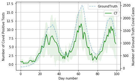
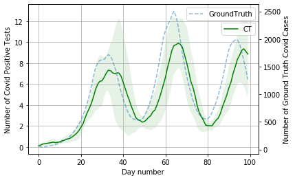
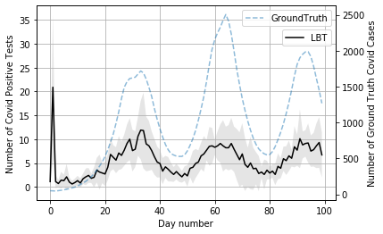
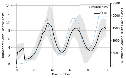
We observe that each testing policy results in three such lockdowns over a hundred day period in our simulation. Interestingly, even with significantly fewer days of lockdown, the reduction in the number of ground truth COVID-19 cases is only marginally less than indefinite lockdown of the previous section. Further, here, too,CT outperforms RST significantly and LBT yields similar performance as CT.

5 Concluding Remarks

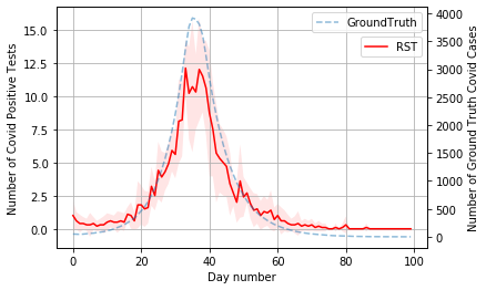
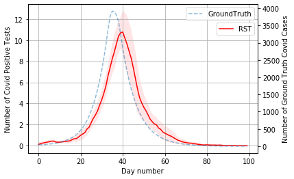
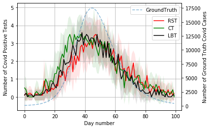
We have taken an initial stab at the question we set to answer: How well do test results reveal the ground truth and help decide when to interventions? Using our simulation framework with 1 test per 2000 people, we have observed that the simplest testing strategy RST captures the trend well. Other strategies such as CT and our proposed LBT yield higher number of positive tests than RST, and are seen to be more effective in enabling interventions. Note that, at the time of writing, this number of daily tests is much higher than what is being done in India. Roughly, 30,000 tests are done daily in India when this article is being written and roughly 1,500 of them happen in the state of Karnataka, the state to which the city of Bengaluru belongs. This amounts to 1 test for about 40,000 people. In fact, even at this low number of tests, positive tests reflect the ground truth trend in our experiments. We conducted experiments with uniform seeding with 5 tests per day (for 100K population) and a shorter experiment with RST alone with 50 tests per day for 1M population; the results are displayed in Figures 22 and 23.

(a) Daily number of tests.

(b) Daily number of tests smoothened by taking an average over a window of 8 days.

Figure 22: Comparative test performance with uniform seeding and without intervention, for a time period of 100 days and with a testing budget of 5 tests/day. Results are averaged across 10 runs and error bars represent 1 standard deviation.

(a) Daily number of tests.

(b) Daily number of tests smoothened by taking an average over a window of 8 days.

Figure 23: Performance of RST with uniform seeding and without intervention for a population of 1 Million, for a time period of 50 days, and with a testing budget of 50 tests/day. Results are averaged across 5 runs and error bars represent 1 standard deviation.

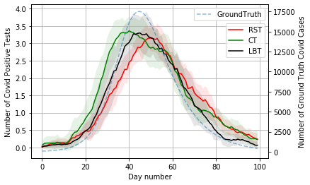
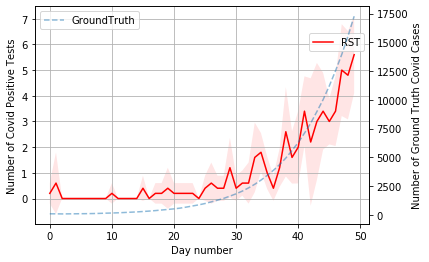
We are tempted to conclude from these observations that India is doing enough daily tests to get a good idea of the ground truth trends. Even with these few tests, a mix of RST and CT, which seems to be the current testing policy for India and many other countries, is a good testing policy. In the initial phase of the spread, perhaps one can control the rapid spread by identifying a large fraction of the infected patients by increasing testing to scale up to the number of infected. But once a significant fraction of population is infected, it may become infeasible to quarantine all the patients. In such a situation, non pharmaceutical interventions such as lockdown are the only option and the role of testing is to get a handle on the ground truth trend. Our simulations suggest that this can be done even with 1 test per 10000 people or so.

But there are a few cautionary remarks we must make: First, the sampling probabilities that emerge during test prescription by doctors in practice are difficult to evaluate and may deviate significantly form our ideal assumptions. Second, our policies rely on symptomatic patients coming out for testing (CT does not assume that). While this can be ensured by an active information campaign and ready access to doctors and digital medical advice, it is important to understand what can happen when a subsection of population is unable to report symptoms. Third, having more positive tests can perhaps offer robustness to deviations from our model in practice.

Finally, we remark that there were many omissions from our initial study. We have not studied gradual ramping-up of test budget, nor have we studied more localized interventions (though our simulations suggest that LBT will be more effective to enable a local lockdown). The effect of under reporting needs to be studied more thoroughly, too. It is of interest also to study extensive testing in an emerging hot-spot as well as pooling for more efficient testing. We plan to consider these issues in later versions of this ongoing work.