Evolutionary dynamics and eigenspectrum of confluent Heun equation

Kavita Jain and Archana Devi
Theoretical Sciences Unit,
Jawaharlal Nehru Centre for Advanced Scientific Research,
Bangalore 560064, India
Abstract

We consider a biological population evolving under the joint action of selection, mutation and random genetic drift. The evolutionary dynamics are described by a one-dimensional Fokker-Planck equation whose eigenfunctions obey a confluent Heun equation. These eigenfunctions are expanded in an infinite series of orthogonal Jacobi polynomials and the expansion coefficients are found to obey a three-term recursion equation. Using scaling ideas, we obtain an expression for the expansion coefficients and an analytical estimate of the number of terms required in the series for an accurate determination of the eigenfunction. The eigenvalue spectrum is studied using a perturbation theory for weak selection and numerically for strong selection. In the latter case, we find that the eigenvalue for the first excited state exhibits a sharp transition: for mutation rate below one, the eigenvalue increases linearly with increasing mutation rate and then remains a constant; higher eigenvalues are found to display a more complex behavior.

Keywords: evolutionary dynamics, confluent Heun equation, eigenspectrum

1 Introduction

Biological evolution has shaped the genetic diversity that we see today on earth [1, 2]. The basic processes that drive evolution include selection, mutation and random genetic drift. While selection decreases the genetic diversity, random mutations increase it. Besides these deterministic processes, stochasticity arising, for example, due to finite carrying capacity plays an important role in determining the evolutionary fate of a population. With growing interest in analyzing the time series data obtained from experiments or field studies [3, 4], and addressing fundamental questions about evolution in changing environments [5], it is important to understand the evolutionary dynamics of a population under the joint action of mutation, selection and genetic drift.

In the absence of selection, the dynamics are completely understood [6], as the Fokker-Planck equation for the distribution of allele frequency obeys the Gauss hypergeometric equation which has the nice property that its Frobenius series expansions lead to two-term recurrence relations for the expansion coefficients and for which the connection formulae that connect its two local solutions are known [7]. But even in the simplest setting where only a single locus in a genome is under selection, the complete evolutionary dynamics are not explicitly known.

In this article, we study the allele frequency distribution in a finite population in which a single, diallelic locus is under time-independent selection and mutations between the two alleles occur at equal rates. To the best of our knowledge, it has not been previously recognized that the eigenfunctions of the Fokker-Planck equation for the frequency distribution obey the confluent Heun equation [8, 9]. This equation has appeared in diverse physical contexts to describe the eigenspectrum of hydrogen molecule ion [10] and quantum Rabi model [11], quasi-normal modes of black holes [12, 13], relaxation dynamics of a polymer [14], etc. Heun equation and its confluent forms are an area of active interest in mathematics community also as the Heun functions generalize the well studied hypergeometric functions. The progress in understanding Heun functions has, however, been slow as Frobenius series or other orthogonal polynomial expansions of this class of equations lead to three-term recurrence relations for the expansion coefficients, and the connection formulae for the local solutions are not explicitly known [15].

For these reasons, here we study the eigenspectrum of the confluent Heun operator of interest, mainly, numerically. As the stationary state corresponding to the zero eigenvalue is exactly known [6], we will focus on the excited states and study them using an orthogonal polynomial expansion of the eigenfunctions. Such an expansion has previously been carried out in [16]; however, these authors obtained a five-term recurrence relation for the expansion coefficients and did not provide any insights into the solution. Here, we obtain a three-term recurrence equation and find that for strong selection, there is a dynamic transition as the relaxation time - which is inversely proportional to the eigenvalue for the first excited state - initially decreases with mutation rate and then becomes a constant at a finite mutation rate. We also show that the expansion coefficients have a scaling form which allows us to estimate the number of terms that contribute significantly to the orthogonal series for the eigenfunctions.

2 Model

We consider a haploid population of N𝑁N individuals that evolves in time according to the standard Moran process [17]. In generation t𝑑t, an individual is chosen to give birth with a probability equal to its fitness relative to that of the population while any individual (including the parent) can die with an equal probability. Thus, if the wild type individual has a fitness 111 and the mutant’s fitness is 1+s1𝑠1+s, the mutant produces a copy of itself with a probability (1+s)​i/wΒ―1𝑠𝑖¯𝑀(1+s)i/{\bar{w}} when i𝑖i mutants are present in the population at time t𝑑t, where w¯​(t)=(1+s)​i+(Nβˆ’i)¯𝑀𝑑1𝑠𝑖𝑁𝑖{\bar{w}}(t)=(1+s)i+(N-i) is the average fitness of the population; similarly, the wild type individual replicates with a probability (Nβˆ’i)/w¯𝑁𝑖¯𝑀(N-i)/{\bar{w}}. After selection and reproduction, an offspring mutates to the other type with a probability u𝑒u. Thus, the population evolves under the joint action of selection, mutation and random genetic drift.

We are interested in understanding the dynamics of the probability distribution of the mutant allele frequency, p=i/N𝑝𝑖𝑁p=i/N in the scaling limit of weak selection, weak mutation (s,uβ†’0→𝑠𝑒0s,u\to 0) and large population size (Nβ†’βˆžβ†’π‘N\to\infty) with finite N​s,N​u𝑁𝑠𝑁𝑒Ns,Nu. Using the mean and the variance of the change in the mutant frequency in the above scaling limits, one can show that the frequency distribution Οˆβ€‹(p,Ο„)πœ“π‘πœ\psi(p,\tau) obeys the following forward Fokker-Planck equation [6, 18],

βˆ‚Οˆβˆ‚Ο„=βˆ’βˆ‚Jβˆ‚p=βˆ’βˆ‚βˆ‚p​[σ​p​qβ€‹Οˆ+μ​(qβˆ’p)β€‹Οˆβˆ’βˆ‚βˆ‚p​(p​qβ€‹Οˆ)],πœ“πœπ½π‘π‘delimited-[]πœŽπ‘π‘žπœ“πœ‡π‘žπ‘πœ“π‘π‘π‘žπœ“\frac{\partial\psi}{\partial\tau}=-\frac{\partial J}{\partial p}=-\frac{\partial}{\partial p}\left[\sigma pq\psi+\mu(q-p)\psi-\frac{\partial}{\partial p}\left(pq\psi\right)\right], (1)

where q=1βˆ’pπ‘ž1𝑝q=1-p is the wild type frequency, J​(p,Ο„)π½π‘πœJ(p,\tau) is the probability current, and Ο„=t/(2​N),ΞΌ=2​N​u,Οƒ=2​N​sformulae-sequenceπœπ‘‘2𝑁formulae-sequenceπœ‡2π‘π‘’πœŽ2𝑁𝑠\tau=t/(2N),\mu=2Nu,\sigma=2Ns are the scaled time, mutation rate and selection rate, respectively. Below we will study the dynamics of the allele frequency distribution subject to the reflecting boundary conditions,

J​(0,Ο„)=J​(1,Ο„)=0,𝐽0𝜏𝐽1𝜏0J(0,\tau)=J(1,\tau)=0, (2)

at all times.

Some comments are in order: in the following, we will assume that sβ‰₯0𝑠0s\geq 0 since for s<0𝑠0s<0, equation (1) is obeyed by the allele frequency qπ‘žq. While the Moran process described above assumes overlapping generations, the Wright-Fisher process for non-overlapping generation also obeys (1) when N𝑁N is replaced by 2​N2𝑁2N. Instead of the forward equation (1), one may study the corresponding backward equation [16]; however, the eigenspectrum of both equations is same [18]. For these reasons, it is sufficient to focus on the above forward equation (1).

We first write Οˆβ€‹(p,Ο„)=βˆ‘β„“=0∞Aℓ​eβˆ’Ξ»β„“β€‹Ο„β€‹Ο•β„“β€‹(p)πœ“π‘πœsuperscriptsubscriptβ„“0subscript𝐴ℓsuperscript𝑒subscriptπœ†β„“πœsubscriptitalic-ϕℓ𝑝\psi(p,\tau)=\sum_{\ell=0}^{\infty}A_{\ell}e^{-\lambda_{\ell}\tau}\phi_{\ell}({p}) where the coefficient Aβ„“subscript𝐴ℓA_{\ell} is determined by the initial condition Οˆβ€‹(p,0)πœ“π‘0\psi(p,0). From (1), we find that the time-independent eigenfunction ϕℓ​(p)subscriptitalic-ϕℓ𝑝\phi_{\ell}(p) obeys the following eigenvalue equation,

βˆ’(σ​p​q​ϕℓ+μ​(qβˆ’p)​ϕℓ)β€²+(p​q​ϕℓ)β€²β€²=βˆ’Ξ»β„“β€‹Ο•β„“,superscriptπœŽπ‘π‘žsubscriptitalic-Ο•β„“πœ‡π‘žπ‘subscriptitalic-Ο•β„“β€²superscriptπ‘π‘žsubscriptitalic-Ο•β„“β€²β€²subscriptπœ†β„“subscriptitalic-Ο•β„“-\left(\sigma pq\phi_{\ell}+\mu(q-p)\phi_{\ell}\right)^{\prime}+\left(pq\phi_{\ell}\right)^{\prime\prime}=-\lambda_{\ell}\phi_{\ell}, (3)

where a prime denotes a derivative with respect to p𝑝p. As the differential operator in (3) is of Sturm-Liouville form [19], we are guaranteed to have real eigenvalues and a complete set of orthonormal eigenfunctions for which

∫01𝑑p​ρ​(p)​ϕℓ​(p)​ϕℓ′​(p)βˆΞ΄β„“,β„“β€²,proportional-tosuperscriptsubscript01differential-dπ‘πœŒπ‘subscriptitalic-ϕℓ𝑝subscriptitalic-Ο•superscriptℓ′𝑝subscript𝛿ℓsuperscriptβ„“β€²\int_{0}^{1}dp\rho(p)\phi_{\ell}(p)\phi_{\ell^{\prime}}(p)\propto\delta_{\ell,\ell^{\prime}}, (4)

where the weight function, ρ​(p)βˆΟ•0βˆ’1proportional-toπœŒπ‘superscriptsubscriptitalic-Ο•01\rho(p)\propto\phi_{0}^{-1} (see below).

In equilibrium where the probability current J𝐽J vanishes for all p𝑝p, the probability distribution is given by [20, 6]

Ο•0​(p)∝(p​q)ΞΌβˆ’1​eσ​p,proportional-tosubscriptitalic-Ο•0𝑝superscriptπ‘π‘žπœ‡1superscriptπ‘’πœŽπ‘\phi_{0}(p)\propto(pq)^{\mu-1}e^{\sigma p}, (5)

where the proportionality constant determined by (4) reduces to the normalization condition ∫01𝑑p​ϕ0​(p)=1superscriptsubscript01differential-d𝑝subscriptitalic-Ο•0𝑝1\int_{0}^{1}dp\phi_{0}(p)=1. For Οƒ=0𝜎0\sigma=0, the above equilibrium distribution is U-shaped for ΞΌ<1πœ‡1\mu<1 and bell-shaped for ΞΌ>1πœ‡1\mu>1; however, for large ΟƒπœŽ\sigma, the stationary distribution Ο•0​(p)subscriptitalic-Ο•0𝑝\phi_{0}(p) for the favored allele peaks close to p=1𝑝1p=1.

3 Confluent Heun equation for the eigenfunctions

We will now focus on (3) which can be rewritten in the standard form as

ϕℓ′′​(p)+(2βˆ’ΞΌpβˆ’1+2βˆ’ΞΌpβˆ’Οƒ)​ϕℓ′​(p)+(Ξ½β„“p+βˆ’2β€‹Οƒβˆ’Ξ½β„“pβˆ’1)​ϕℓ​(p)=0,superscriptsubscriptitalic-ϕℓ′′𝑝2πœ‡π‘12πœ‡π‘πœŽsuperscriptsubscriptitalic-ϕℓ′𝑝subscriptπœˆβ„“π‘2𝜎subscriptπœˆβ„“π‘1subscriptitalic-ϕℓ𝑝0\phi_{\ell}^{\prime\prime}(p)+\left(\frac{2-\mu}{p-1}+\frac{2-\mu}{p}-\sigma\right)\phi_{\ell}^{\prime}(p)+\left(\frac{\nu_{\ell}}{p}+\frac{-2\sigma-\nu_{\ell}}{p-1}\right)\phi_{\ell}(p)=0, (6)

where Ξ½β„“=2β€‹ΞΌβˆ’Οƒβˆ’2+Ξ»β„“subscriptπœˆβ„“2πœ‡πœŽ2subscriptπœ†β„“\nu_{\ell}=2\mu-\sigma-2+\lambda_{\ell}. Equation (6) is a (singly) confluent Heun equation which has regular singular points at p=0,1𝑝01p=0,1 and an irregular singularity of rank 111 at infinite p𝑝p [8, 21, 9]. The following special cases of (6) are known [6]: for Οƒ=0𝜎0\sigma=0 (no selection), (6) reduces to the Gauss hypergeometric equation which has regular singular points at zero, one and infinity, and for Οƒ=ΞΌ=0πœŽπœ‡0\sigma=\mu=0 (only genetic drift), the eigenfunction Ο•β„“subscriptitalic-Ο•β„“\phi_{\ell} obeys the Gegenbauer equation. For nonzero selection but zero mutation rate, Vℓ​(z)=eβˆ’Οƒβ€‹p/2​ϕℓ​(p)subscript𝑉ℓ𝑧superscriptπ‘’πœŽπ‘2subscriptitalic-ϕℓ𝑝V_{\ell}(z)=e^{-\sigma p/2}\phi_{\ell}(p) with p=(1βˆ’z)/2𝑝1𝑧2p=(1-z)/2 obeys the oblate spheroidal equation [22]. However, except for the stationary state (5) corresponding to eigenvalue zero, neither the eigenvalue spectrum nor the eigenfunctions are known for the above confluent Heun differential operator.

The general solution of (6) can be expanded as a Frobenius series about p=0𝑝0p=0 [23] which, on imposing the reflecting boundary condition (2) at p=0𝑝0p=0 gives ϕℓ​(p)=pΞΌβˆ’1​Fℓ​(p)subscriptitalic-ϕℓ𝑝superscriptπ‘πœ‡1subscript𝐹ℓ𝑝\phi_{\ell}(p)=p^{\mu-1}F_{\ell}(p) for |p|<1,ΞΌ>0formulae-sequence𝑝1πœ‡0|p|<1,{\mu>0} where Fβ„“subscript𝐹ℓF_{\ell} is an analytic function (see AppendixΒ A). Due to the self-adjoint nature of the Heun operator, we can expand Fβ„“subscript𝐹ℓF_{\ell} as a linear combination of suitable orthogonal functions [19]; a power series expansion of Fβ„“subscript𝐹ℓF_{\ell} is given in AppendixΒ A.

An orthogonal expansion of (6) with boundary conditions (2) has been carried out in [16] by writing the distribution function, ϕℓ​(p)=βˆ‘na^n(β„“)​G^n​(p)subscriptitalic-ϕℓ𝑝subscript𝑛superscriptsubscript^π‘Žπ‘›β„“subscript^𝐺𝑛𝑝\phi_{\ell}(p)=\sum_{n}{\hat{a}}_{n}^{(\ell)}{\hat{G}}_{n}(p) where G^n=(p​q)ΞΌβˆ’1​eσ​p/2​Pn(ΞΌβˆ’1,ΞΌβˆ’1)​(1βˆ’2​p)subscript^𝐺𝑛superscriptπ‘π‘žπœ‡1superscriptπ‘’πœŽπ‘2superscriptsubscriptπ‘ƒπ‘›πœ‡1πœ‡112𝑝{\hat{G}}_{n}=(pq)^{\mu-1}e^{\sigma p/2}P_{n}^{(\mu-1,\mu-1)}(1-2p) and Pn(Ξ±,Ξ²)​(x)superscriptsubscript𝑃𝑛𝛼𝛽π‘₯P_{n}^{(\alpha,\beta)}(x) denotes Jacobi polynomial of order n𝑛n that obey the following orthogonality relation [24],

βˆ«βˆ’11𝑑x​(1βˆ’x)α​(1+x)β​Pn(Ξ±,Ξ²)​(x)​Pnβ€²(Ξ±,Ξ²)​(x)=hn​δn,nβ€².superscriptsubscript11differential-dπ‘₯superscript1π‘₯𝛼superscript1π‘₯𝛽superscriptsubscript𝑃𝑛𝛼𝛽π‘₯superscriptsubscript𝑃superscript𝑛′𝛼𝛽π‘₯subscriptβ„Žπ‘›subscript𝛿𝑛superscript𝑛′\int_{-1}^{1}dx(1-x)^{\alpha}(1+x)^{\beta}P_{n}^{(\alpha,\beta)}(x)P_{n^{\prime}}^{(\alpha,\beta)}(x)=h_{n}\delta_{n,n^{\prime}}. (7)

The above G^nsubscript^𝐺𝑛{\hat{G}}_{n} has the property that they are orthogonal with respect to the same weight function as that for Ο•β„“subscriptitalic-Ο•β„“\phi_{\ell}, namely, ρ𝜌\rho. But this choice leads to a 555-term recursion relation for the coefficients a^n(β„“)superscriptsubscript^π‘Žπ‘›β„“{\hat{a}}_{n}^{(\ell)} that are not amenable to analytical calculations.

Here, we write ϕℓ​(p)=βˆ‘nan(β„“)​Gnsubscriptitalic-ϕℓ𝑝subscript𝑛superscriptsubscriptπ‘Žπ‘›β„“subscript𝐺𝑛\phi_{\ell}(p)=\sum_{n}a_{n}^{(\ell)}G_{n} with Gn=(p​q)ΞΌβˆ’1​Pn(ΞΌβˆ’1,ΞΌβˆ’1)​(1βˆ’2​p)subscript𝐺𝑛superscriptπ‘π‘žπœ‡1superscriptsubscriptπ‘ƒπ‘›πœ‡1πœ‡112𝑝G_{n}=(pq)^{\mu-1}P_{n}^{(\mu-1,\mu-1)}(1-2p) that, as can be verified using (7), are orthogonal with respect to the weight function (p​q)1βˆ’ΞΌsuperscriptπ‘π‘ž1πœ‡(pq)^{1-\mu}. As detailed in AppendixΒ B, our choice of the orthogonal basis leads to 3-term recursion relations for an(β„“)superscriptsubscriptπ‘Žπ‘›β„“a_{n}^{(\ell)} (see also [14]), and we can write

ϕℓ​(p)=(p​q)ΞΌβˆ’1β€‹βˆ‘n=1∞cn(β„“)​Γ​(n)Γ​(n+ΞΌβˆ’1)​Pnβˆ’1(ΞΌβˆ’1,ΞΌβˆ’1)​(1βˆ’2​p),subscriptitalic-ϕℓ𝑝superscriptπ‘π‘žπœ‡1superscriptsubscript𝑛1superscriptsubscriptπ‘π‘›β„“Ξ“π‘›Ξ“π‘›πœ‡1superscriptsubscript𝑃𝑛1πœ‡1πœ‡112𝑝\phi_{\ell}(p)=(pq)^{\mu-1}\sum_{n=1}^{\infty}c_{n}^{(\ell)}\frac{\Gamma(n)}{\Gamma(n+\mu-1)}P_{n-1}^{(\mu-1,\mu-1)}(1-2p), (8)

which satisfies the boundary condition (2) at p=1𝑝1p=1 also. The expansion coefficients cn(β„“)superscriptsubscript𝑐𝑛ℓc_{n}^{(\ell)}’s are determined recursively through the following equations,

λℓ​c1(β„“)subscriptπœ†β„“superscriptsubscript𝑐1β„“\displaystyle{\lambda}_{\ell}c_{1}^{(\ell)} =\displaystyle= 0,0\displaystyle 0, (9)
Tβˆ’β€‹(n)​cnβˆ’1(β„“)+T0​(n)​cn(β„“)+T+​(n)​cn+1(β„“)subscript𝑇𝑛superscriptsubscript𝑐𝑛1β„“subscript𝑇0𝑛superscriptsubscript𝑐𝑛ℓsubscript𝑇𝑛superscriptsubscript𝑐𝑛1β„“\displaystyle T_{-}(n)c_{n-1}^{(\ell)}+T_{0}(n)c_{n}^{(\ell)}+T_{+}(n)c_{n+1}^{(\ell)} =\displaystyle= βˆ’Ξ»β„“β€‹cn(β„“),nβ‰₯2,subscriptπœ†β„“superscriptsubscript𝑐𝑛ℓ𝑛2\displaystyle-\lambda_{\ell}c_{n}^{(\ell)}~{},~{}n\geq 2, (10)

where

Tβˆ’β€‹(n)subscript𝑇𝑛\displaystyle T_{-}(n) =\displaystyle= σ​(2​μ+nβˆ’2)​(2​μ+nβˆ’3)10βˆ’4β€‹ΞΌβˆ’4​n<0,𝜎2πœ‡π‘›22πœ‡π‘›3104πœ‡4𝑛0\displaystyle\frac{\sigma(2\mu+n-2)(2\mu+n-3)}{10-4\mu-4n}<0, (11)
T+​(n)subscript𝑇𝑛\displaystyle T_{+}(n) =\displaystyle= σ​n​(1βˆ’n)2βˆ’4β€‹ΞΌβˆ’4​n>0,πœŽπ‘›1𝑛24πœ‡4𝑛0\displaystyle\frac{\sigma n(1-n)}{2-4\mu-4n}>0, (12)
T0​(n)subscript𝑇0𝑛\displaystyle T_{0}(n) =\displaystyle= (1βˆ’n)​(2​μ+nβˆ’2)<0.1𝑛2πœ‡π‘›20\displaystyle(1-n)(2\mu+n-2)<0. (13)

As already stated, the stationary state corresponding to Ξ»0=0subscriptπœ†00\lambda_{0}=0 is given by (5) and it can be used to find the expansion coefficients cn(0)superscriptsubscript𝑐𝑛0c_{n}^{(0)}, as described in AppendixΒ C. In the following, we are interested in excited states with nonzero eigenvalues; due to (9), this means that c1(β„“)=0superscriptsubscript𝑐1β„“0c_{1}^{(\ell)}=0 for β„“=1,2,…ℓ12…\ell=1,2,.... Furthermore, for large n𝑛n, the ratio rn=cn+1/cnsubscriptπ‘Ÿπ‘›subscript𝑐𝑛1subscript𝑐𝑛r_{n}=c_{n+1}/c_{n} has following linearly independent solutions,

rn+∼4​nΟƒ,rnβˆ’βˆΌβˆ’Οƒ4​nformulae-sequencesimilar-tosuperscriptsubscriptπ‘Ÿπ‘›4π‘›πœŽsimilar-tosuperscriptsubscriptπ‘Ÿπ‘›πœŽ4𝑛r_{n}^{+}\sim\frac{4n}{\sigma},~{}~{}r_{n}^{-}\sim-\frac{\sigma}{4n} (14)

for any β„“β„“\ell. As the (minimal) solution rnβˆ’superscriptsubscriptπ‘Ÿπ‘›r_{n}^{-} ensures the convergence of the continued fraction method for evaluating eigenvalues [25] (see also Sec.Β 4), we have the boundary condition that the expansion coefficients vanish at large n𝑛n.

In summary, (10) along with boundary conditions c1(β„“),cK+2β†’βˆž(β„“)=0superscriptsubscript𝑐1β„“superscriptsubscript𝑐→𝐾2β„“0c_{1}^{(\ell)},c_{K+2\to\infty}^{(\ell)}=0 defines an eigenvalue problem, 𝐓​cβ†’(β„“)=βˆ’Ξ»β„“β€‹cβ†’(β„“),β„“β‰₯1formulae-sequence𝐓superscript→𝑐ℓsubscriptπœ†β„“superscript→𝑐ℓℓ1{\bf T}\vec{c}^{(\ell)}=-\lambda_{\ell}\vec{c}^{(\ell)},\ell\geq 1 for eigenvector cβ†’(β„“)superscript→𝑐ℓ\vec{c}^{(\ell)} and eigenvalue βˆ’Ξ»β„“subscriptπœ†β„“-\lambda_{\ell} where 𝐓𝐓{\bf T} is K𝐾K-dimensional square matrix.

4 Eigenvalue problem: numerical analysis

For the ratio rn(β„“)superscriptsubscriptπ‘Ÿπ‘›β„“r_{n}^{(\ell)}, the recursion equation (10) can be written as

rnβˆ’1(β„“)=jnkn+rn(β„“)=jnkn+jn+1kn+1+rn+1(β„“),superscriptsubscriptπ‘Ÿπ‘›1β„“subscript𝑗𝑛subscriptπ‘˜π‘›superscriptsubscriptπ‘Ÿπ‘›β„“subscript𝑗𝑛subscriptπ‘˜π‘›subscript𝑗𝑛1subscriptπ‘˜π‘›1superscriptsubscriptπ‘Ÿπ‘›1β„“r_{n-1}^{(\ell)}=\frac{j_{n}}{k_{n}+r_{n}^{(\ell)}}=\frac{j_{n}}{k_{n}+\frac{j_{n+1}}{k_{n+1}+r_{n+1}^{(\ell)}}}, (15)

where jn=βˆ’Tβˆ’β€‹(n)/T+​(n)subscript𝑗𝑛subscript𝑇𝑛subscript𝑇𝑛j_{n}=-T_{-}(n)/T_{+}(n) and kn(β„“)=(T0​(n)+Ξ»β„“)/T+​(n)superscriptsubscriptπ‘˜π‘›β„“subscript𝑇0𝑛subscriptπœ†β„“subscript𝑇𝑛k_{n}^{(\ell)}=(T_{0}(n)+\lambda_{\ell})/T_{+}(n). Continuing in this manner, we have

r2(β„“)=j3k3(β„“)+j4k4(β„“)+j5k5(β„“)+…=βˆ’k2(β„“),superscriptsubscriptπ‘Ÿ2β„“continued-fractionsubscript𝑗3superscriptsubscriptπ‘˜3β„“continued-fractionsubscript𝑗4superscriptsubscriptπ‘˜4β„“continued-fractionsubscript𝑗5superscriptsubscriptπ‘˜5ℓ…superscriptsubscriptπ‘˜2β„“r_{2}^{(\ell)}=\cfrac{j_{3}}{k_{3}^{(\ell)}+\cfrac{j_{4}}{k_{4}^{(\ell)}+\cfrac{j_{5}}{k_{5}^{(\ell)}+...}}}=-k_{2}^{(\ell)}, (16)

where we have used the boundary condition c1(β„“)=0,β„“>0formulae-sequencesuperscriptsubscript𝑐1β„“0β„“0c_{1}^{(\ell)}=0,\ell>0. Starting from rnβˆ’superscriptsubscriptπ‘Ÿπ‘›r_{n}^{-} in (14), the above continued fraction was used to calculate Ξ»β„“subscriptπœ†β„“\lambda_{\ell} and rn(β„“)superscriptsubscriptπ‘Ÿπ‘›β„“r_{n}^{(\ell)} numerically [25], and we found the ratio rn(β„“)superscriptsubscriptπ‘Ÿπ‘›β„“r_{n}^{(\ell)} to be negative for all n𝑛n. From these ratio of expansion coefficients, the eigenfunction ϕℓ​(p)subscriptitalic-ϕℓ𝑝\phi_{\ell}(p) was obtained by carrying out the sum over K+1𝐾1K+1 terms in (8). One can also diagonalize matrix 𝐓𝐓{\bf T} to find eigenvalues and eigenfunctions. To obtain numerical results, both these methods were applied to finite-dimensional matrix 𝐓𝐓{\bf T} of large size K𝐾K.

4.1 Eigenvalues

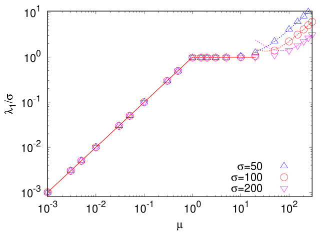
FigureΒ 1 shows the numerical results for the eigenvalue Ξ»1subscriptπœ†1\lambda_{1} as a function of the mutation rate ΞΌπœ‡\mu and large selection strengths. For μ≫σmuch-greater-thanπœ‡πœŽ\mu\gg\sigma where selection is weak relative to mutation, the eigenvalue varies with ΞΌπœ‡\mu essentially the same way as that in the absence of selection since, as discussed in Sec.Β 5, the correction to Ξ»1subscriptπœ†1\lambda_{1} due to selection is quadratic in Οƒ/ΞΌπœŽπœ‡\sigma/\mu. But for ΞΌβ‰ͺΟƒmuch-less-thanπœ‡πœŽ\mu\ll\sigma, the eigenvalue increases linearly with ΟƒπœŽ\sigma (see Sec.Β 6), and our numerical results in Fig.Β 1 suggest that

Ξ»1ΟƒβŸΆΟƒβ†’βˆž{ΞΌ,μ≀11,ΞΌ>1.superscriptβŸΆβ†’πœŽsubscriptπœ†1𝜎casesπœ‡πœ‡11πœ‡1\frac{\lambda_{1}}{\sigma}\stackrel{{\scriptstyle\sigma\to\infty}}{{\longrightarrow}}\begin{cases}\mu,&\mu\leq 1\\ 1,&\mu>1\end{cases}. (17)

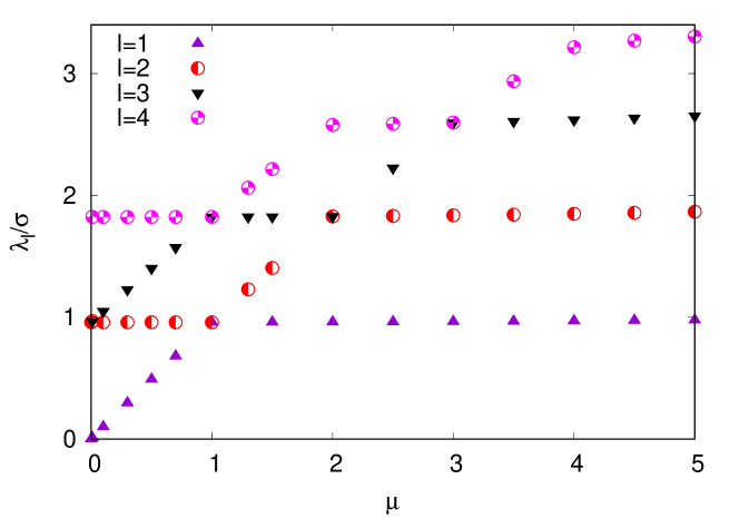
We have also studied the corrections to the above conjectured eigenvalue, and find that they approach the asymptotic values as 1/Οƒ1𝜎1/\sigma (data not shown). The higher eigenvalues shown in Fig.Β 2 exhibit a more complex behavior. The eigenvalue Ξ»2subscriptπœ†2\lambda_{2} remains a constant for ΞΌ<1πœ‡1\mu<1, increases linearly for 1<ΞΌ<21πœ‡21<\mu<2 and is a constant for ΞΌβ‰₯2πœ‡2\mu\geq 2; a similar pattern is seen for Ξ»3subscriptπœ†3\lambda_{3} and Ξ»4subscriptπœ†4\lambda_{4}.

4.2 Eigenfunctions

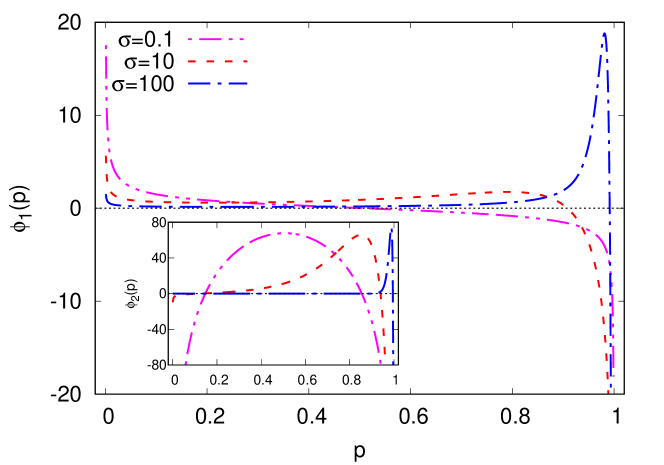
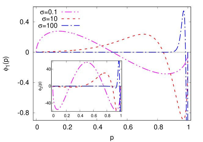
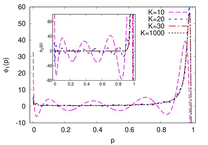
Figure 3 shows the numerical results for the eigenfunctions Ο•1​(p)subscriptitalic-Ο•1𝑝\phi_{1}(p) and Ο•2​(p)subscriptitalic-Ο•2𝑝\phi_{2}(p) for various values of ΟƒπœŽ\sigma and large K𝐾K. As expected, the β„“β„“\ellth excited state has β„“β„“\ell nodes whose location depends on ΞΌπœ‡\mu and ΟƒπœŽ\sigma. Other than this feature, the distribution is qualitatively similar to that in the stationary state given by (5). When selection is absent, the eigenfunctions are symmetric about p=1/2𝑝12p=1/2 [6]; for this reason, the first excited state for small σ≲1less-than-or-similar-to𝜎1\sigma\lesssim 1 has a node close to one half. But for stronger selection, the eigenstate is highly asymmetric and as in the stationary state, the excited states also peak close to the allele frequency equal to one.

5 Weak selection limit

As the eigenvalues are known exactly for Οƒ=0𝜎0\sigma=0 [6], we can use a perturbation theory to determine Ξ»β„“subscriptπœ†β„“\lambda_{\ell}’s for Οƒβ‰ͺΞΌmuch-less-thanπœŽπœ‡\sigma\ll\mu. On expanding the coefficient cn(β„“)superscriptsubscript𝑐𝑛ℓc_{n}^{(\ell)} and eigenvalue Ξ»β„“subscriptπœ†β„“\lambda_{\ell} in a power series to quadratic orders in ΟƒπœŽ\sigma and substituting them in (10), we find that the zeroth order term in ΟƒπœŽ\sigma yields λℓ​(Οƒ=0)=ℓ​(2​μ+β„“βˆ’1),β„“=0,1,…formulae-sequencesubscriptπœ†β„“πœŽ0β„“2πœ‡β„“1β„“01…\lambda_{\ell}(\sigma=0)=\ell(2\mu+\ell-1),\ell=0,1,... [6]. The first order correction to the eigenvalue is found to be zero and the quadratic term in ΟƒπœŽ\sigma leads to

λℓ​(Οƒ)β‰ˆΞ»β„“β€‹(Οƒ=0)+T+​(β„“+1)​Tβˆ’β€‹(β„“+2)T0​(β„“+2)βˆ’T0​(β„“+1)+T+​(β„“)​Tβˆ’β€‹(β„“+1)T0​(β„“)βˆ’T0​(β„“+1).subscriptπœ†β„“πœŽsubscriptπœ†β„“πœŽ0subscript𝑇ℓ1subscript𝑇ℓ2subscript𝑇0β„“2subscript𝑇0β„“1subscript𝑇ℓsubscript𝑇ℓ1subscript𝑇0β„“subscript𝑇0β„“1\lambda_{\ell}(\sigma)\approx\lambda_{\ell}(\sigma=0)+\frac{T_{+}(\ell+1)T_{-}(\ell+2)}{T_{0}(\ell+2)-T_{0}(\ell+1)}+\frac{T_{+}(\ell)T_{-}(\ell+1)}{T_{0}(\ell)-T_{0}(\ell+1)}. (18)

From the above expression, we obtain the eigenvalue for the first excited state to be

Ξ»1β‰ˆ2​μ+Οƒ2​μ(2​μ+2)​(2​μ+3),subscriptπœ†12πœ‡superscript𝜎2πœ‡2πœ‡22πœ‡3\lambda_{1}\approx 2\mu+\frac{\sigma^{2}\mu}{(2\mu+2)(2\mu+3)}, (19)

which is in good agreement with the numerical data in Fig.Β 1. Equation (18) also shows that as for Οƒ=0𝜎0\sigma=0, the gap between the consecutive eigenvalues increases with index β„“β„“\ell.

6 Strong selection limit

We now turn to the strong selection regime where σ≫μmuch-greater-thanπœŽπœ‡\sigma\gg\mu. The coefficient (T0​(n)+Ξ»β„“)/Οƒsubscript𝑇0𝑛subscriptπœ†β„“πœŽ(T_{0}(n)+\lambda_{\ell})/\sigma of cn(β„“)superscriptsubscript𝑐𝑛ℓc_{n}^{(\ell)} in (10) shows that for Οƒβ†’βˆžβ†’πœŽ\sigma\to\infty, a nontrivial eigenvalue for the excited states is obtained if Ξ»β„“subscriptπœ†β„“\lambda_{\ell} scales linearly with ΟƒπœŽ\sigma, in accordance with the numerical results shown in Fig.Β 1. One is then tempted to ignore the T0subscript𝑇0T_{0} term altogether; however, as explained in AppendixΒ D, this results in imaginary eigenvalues for any K𝐾K. The correct limit procedure for strong selection is therefore to take Kβ†’βˆžβ†’πΎK\to\infty followed by Οƒβ†’βˆžβ†’πœŽ\sigma\to\infty. In Sec.Β 6.1 and Sec.Β 6.2, we find the expansion coefficients for large and small n𝑛n, respectively, for large, finite ΟƒπœŽ\sigma when Kβ†’βˆžβ†’πΎK\to\infty. Our analysis, however, does not yield eigenvalues that were studied in Sec.Β 4 numerically.

6.1 Scaling form for the expansion coefficients

Although we have not been able to obtain the eigenvalues analytically, a simple but accurate approximation for the coefficients cn(β„“),n≫1much-greater-thansuperscriptsubscript𝑐𝑛ℓ𝑛1c_{n}^{(\ell)},n\gg 1 for large ΟƒπœŽ\sigma can be obtained as follows. We again consider the coefficient T0​(n)+Ξ»β„“subscript𝑇0𝑛subscriptπœ†β„“T_{0}(n)+\lambda_{\ell} of cn(β„“)superscriptsubscript𝑐𝑛ℓc_{n}^{(\ell)}: for large ΟƒπœŽ\sigma, T0∼n2similar-tosubscript𝑇0superscript𝑛2T_{0}\sim n^{2} can be neglected in comparison to Ξ»β„“βˆΌΟƒsimilar-tosubscriptπœ†β„“πœŽ\lambda_{\ell}\sim\sigma when nβ‰ͺΟƒmuch-less-thanπ‘›πœŽn\ll\sqrt{\sigma}, and as a consequence, the expansion coefficient cn(β„“)superscriptsubscript𝑐𝑛ℓc_{n}^{(\ell)} is independent of ΟƒπœŽ\sigma for small n𝑛n. But the eigenvalue can be ignored for n≫σmuch-greater-thanπ‘›πœŽn\gg\sqrt{\sigma} and we may expect a ΟƒπœŽ\sigma-dependence for cn(β„“)superscriptsubscript𝑐𝑛ℓc_{n}^{(\ell)} when n𝑛n is large. These observations suggest that for σ≫1much-greater-than𝜎1\sigma\gg 1, the coefficient |cn(β„“)|superscriptsubscript𝑐𝑛ℓ|c_{n}^{(\ell)}| is of a scaling form,

|cn(β„“)||c2(β„“)|=CΟƒ,μ​fℓ​(nΟƒ),superscriptsubscript𝑐𝑛ℓsuperscriptsubscript𝑐2β„“subscriptπΆπœŽπœ‡subscriptπ‘“β„“π‘›πœŽ\frac{|c_{n}^{(\ell)}|}{|c_{2}^{(\ell)}|}=C_{\sigma,\mu}f_{\ell}\left(\frac{n}{\sqrt{\sigma}}\right), (20)

where the ΟƒπœŽ\sigma-dependence of C𝐢C is fixed using that the |cn(β„“)|superscriptsubscript𝑐𝑛ℓ|c_{n}^{(\ell)}| must be independent of ΟƒπœŽ\sigma for small n𝑛n.

Since the cn(β„“)superscriptsubscript𝑐𝑛ℓc_{n}^{(\ell)}’s have alternating signs, (10) gives

Tβˆ’β€‹(n)​|cnβˆ’1(β„“)|+T+​(n)​|cn+1(β„“)|=(T0​(n)+Ξ»β„“)​|cn(β„“)|,nβ‰₯2.formulae-sequencesubscript𝑇𝑛superscriptsubscript𝑐𝑛1β„“subscript𝑇𝑛superscriptsubscript𝑐𝑛1β„“subscript𝑇0𝑛subscriptπœ†β„“superscriptsubscript𝑐𝑛ℓ𝑛2T_{-}(n)|c_{n-1}^{(\ell)}|+T_{+}(n)|c_{n+1}^{(\ell)}|=(T_{0}(n)+\lambda_{\ell})|c_{n}^{(\ell)}|~{},~{}n\geq 2. (21)

Using the scaling form (20) in the above equation and collecting terms to order ΟƒπœŽ\sigma, we arrive at a first order linear differential equation for the scaling function fℓ​(u)subscript𝑓ℓ𝑒f_{\ell}(u) given by (see also AppendixΒ D)

u2​fℓ′​(u)+(u2βˆ’ΞΌβˆ’ΞΊβ„“+12)​fℓ​(u)=0,𝑒2superscriptsubscript𝑓ℓ′𝑒superscript𝑒2πœ‡subscriptπœ…β„“12subscript𝑓ℓ𝑒0\frac{u}{2}f_{\ell}^{\prime}(u)+\left(u^{2}-\mu-\kappa_{\ell}+\frac{1}{2}\right)f_{\ell}(u)=0, (22)

where ΞΊβ„“=limΟƒβ†’βˆžΞ»β„“/Οƒsubscriptπœ…β„“subscriptβ†’πœŽsubscriptπœ†β„“πœŽ\kappa_{\ell}=\lim_{\sigma\to\infty}{\lambda_{\ell}}/{\sigma}. On solving the above differential equation, we find that

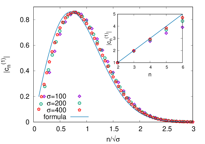
|cn(β„“)|β‰ˆCμ​n2​μ+2β€‹ΞΊβ„“βˆ’1​eβˆ’n2/Οƒ.superscriptsubscript𝑐𝑛ℓsubscriptπΆπœ‡superscript𝑛2πœ‡2subscriptπœ…β„“1superscript𝑒superscript𝑛2𝜎|c_{n}^{(\ell)}|\approx C_{\mu}n^{2\mu+2\kappa_{\ell}-1}e^{-{n^{2}}/{\sigma}}. (23)

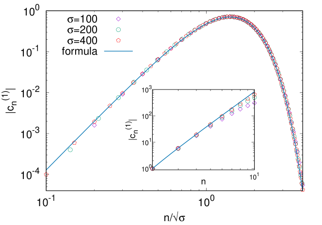
In Fig.Β 4, the numerically obtained expansion coefficients |cn(1)|superscriptsubscript𝑐𝑛1|c_{n}^{(1)}| and the above expression along with the conjectured eigenvalue (17) for the first excited state are compared and we find a very good agreement, except for small n𝑛n where the scaling limit is not valid. Equation (22) also shows that the scaling function fℓ​(u)subscript𝑓ℓ𝑒f_{\ell}(u) has a turning point at uβ„“βˆ—=ΞΌ+ΞΊβ„“βˆ’12subscriptsuperscriptπ‘’β„“πœ‡subscriptπœ…β„“12u^{*}_{\ell}=\sqrt{\mu+\kappa_{\ell}-\frac{1}{2}}; for the first excited state, using the conjecture (17), we find that |cn(1)|superscriptsubscript𝑐𝑛1|c_{n}^{(1)}| is a nonmonotonic function for ΞΌ>1/4πœ‡14\mu>1/4 and decreases monotonically otherwise. We have numerically verified that (23) works well for higher excited states also (data not shown).

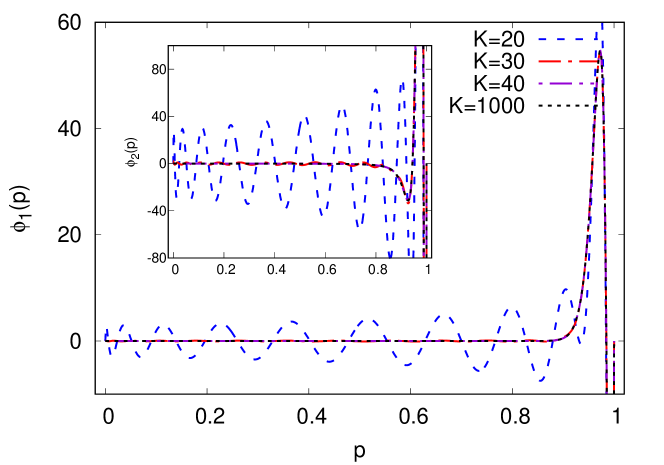
Equation (23) suggests that as the expansion coefficients decay fast for large n𝑛n, it may be sufficient to keep terms up to n≲σless-than-or-similar-toπ‘›πœŽn\lesssim\sqrt{\sigma} for the evaluation of sum (8) for the eigenfunction. This expectation is tested in Fig.Β 5 for two eigenfunctions, and we find that when the sum is terminated at small KβˆΌΟƒsimilar-to𝐾𝜎K\sim\sqrt{\sigma}, the result matches well with those obtained with K≫σmuch-greater-than𝐾𝜎K\gg\sigma. We remark that at small K𝐾K, the eigenfunction is seen to have several nodes. But, as already shown in Fig.Β 3, the eigenfunction ϕℓ​(p)subscriptitalic-ϕℓ𝑝\phi_{\ell}(p) has β„“β„“\ell nodes for large enough K𝐾K.

6.2 Expansion coefficients for infinite selection

As shown in Fig.Β 4, the expansion coefficients in (23) do not match with the numerical results for small n𝑛n. Here, we show that these can be found exactly for special values of ΞΌπœ‡\mu. For this purpose, it is useful to define

dn(β„“)=|cn(β„“)6βˆ’4β€‹ΞΌβˆ’4​n|,nβ‰₯2.d_{n}^{(\ell)}=\bigg{\rvert}\frac{c_{n}^{(\ell)}}{6-4\mu-4n}\bigg{\rvert}~{},~{}n\geq 2. (24)

As shown in AppendixΒ D, the generating function π’Ÿβ„“β€‹(z)=βˆ‘n=2∞dn(β„“)​znsubscriptπ’Ÿβ„“π‘§superscriptsubscript𝑛2superscriptsubscript𝑑𝑛ℓsuperscript𝑧𝑛{\cal D}_{\ell}(z)=\sum_{n=2}^{\infty}d_{n}^{(\ell)}z^{n} obeys a third order differential equation given by (D.2); however, for Οƒβ†’βˆžβ†’πœŽ\sigma\to\infty, we obtain

π’Ÿβ„“β€‹(z)={z4​κℓ​((1+z1βˆ’z)2β€‹ΞΊβ„“βˆ’1)(ΞΌ=1/2)(z1βˆ’z2)2​(1+z1βˆ’z)2​κℓ(ΞΌ=3/2)subscriptπ’Ÿβ„“π‘§cases𝑧4subscriptπœ…β„“superscript1𝑧1𝑧2subscriptπœ…β„“1πœ‡12superscript𝑧1superscript𝑧22superscript1𝑧1𝑧2subscriptπœ…β„“πœ‡32{\cal D}_{\ell}(z)=\begin{cases}\frac{z}{4\kappa_{\ell}}\left(\left(\frac{1+z}{1-z}\right)^{2\kappa_{\ell}}-1\right)&~{}~{}(\mu=1/2)\\ \left(\frac{z}{1-z^{2}}\right)^{2}\left(\frac{1+z}{1-z}\right)^{2\kappa_{\ell}}&~{}~{}(\mu=3/2)\end{cases} (25)

on choosing d2(β„“)=1superscriptsubscript𝑑2β„“1d_{2}^{(\ell)}=1. Using the conjecture (17), we get

|cn(1)||c2(1)|βŸΆΟƒβ†’βˆž{nβˆ’1(ΞΌ=1/2)n2​(n2βˆ’1)12(ΞΌ=3/2),superscriptβŸΆβ†’πœŽsuperscriptsubscript𝑐𝑛1superscriptsubscript𝑐21cases𝑛1πœ‡12superscript𝑛2superscript𝑛2112πœ‡32\frac{|c_{n}^{(1)}|}{|c_{2}^{(1)}|}\stackrel{{\scriptstyle\sigma\to\infty}}{{\longrightarrow}}\begin{cases}n-1&~{}~{}(\mu=1/2)\\ \frac{n^{2}(n^{2}-1)}{12}&~{}~{}(\mu=3/2)\end{cases}, (26)

which are consistent with the power law scaling in (23) and the numerical data in the inset of Fig.Β 4 for small n𝑛n.

7 Discussion

While the confluent Heun equation frequently appears in various problems in physics [9], here, for the first time, we have made a connection between this equation and a standard population-genetics model defined by (1). This relationship is useful, especially for biologists [26, 27, 3], as one can simply use the standard packages (such as Maple and latest version of Mathematica) to solve the partial differential equation (1) numerically. However, in [16] and here, an orthogonal series expansion is used to recast the problem as an eigenvalue problem (10) which can also be easily implemented numerically and is, perhaps, more amenable to analysis (see, for e.g., [12]).

Here we have studied the eigenvalues and eigenfunctions of the confluent Heun operator in some detail. Our main result for the first eigenvalue Ξ»1subscriptπœ†1\lambda_{1} which is inversely proportional to the relaxation time is summarized in Fig.Β 1. For strong selection (σ≫μmuch-greater-thanπœŽπœ‡\sigma\gg\mu), we find that there is a transition at mutation rate ΞΌ=1πœ‡1\mu=1 and the eigenvalue Ξ»1subscriptπœ†1\lambda_{1} is independent of mutation rate for 1<ΞΌβ‰ͺΟƒ1πœ‡much-less-than𝜎1<\mu\ll\sigma. In contrast, in the absence of selection, the relaxation time decreases monotonically as 1/ΞΌ1πœ‡1/\mu [6].

Although we have produced strong numerical evidence for the behavior of the eigenvalues with model parameters, for the reasons described in Sec.Β 1, it seems very difficult to make analytical progress. However, in the limit of strong selection, an analytical understanding of (17), perhaps using a WKB approximation [28], may be possible.

Appendix A Frobenius series expansion

Since p=0𝑝0p=0 is a regular singular point of the confluent Heun equation, we can expand the eigenfunction in a Frobenius series by writing ϕℓ​(p)=paβ€‹βˆ‘n=0∞fn(β„“)​pn,|p|<1formulae-sequencesubscriptitalic-ϕℓ𝑝superscriptπ‘π‘Žsuperscriptsubscript𝑛0superscriptsubscript𝑓𝑛ℓsuperscript𝑝𝑛𝑝1\phi_{\ell}(p)=p^{a}\sum_{n=0}^{\infty}f_{n}^{(\ell)}p^{n},|p|<1 [19]. Substituting it in (6) and setting the coefficient of paβˆ’1superscriptπ‘π‘Ž1p^{a-1} to zero, we find the indicial exponents to be a=0π‘Ž0a=0 and ΞΌβˆ’1πœ‡1\mu-1. For ΞΌβ‰ 1πœ‡1\mu\neq 1, the eigenfunction can be written as

ϕℓ​(p)=a~1​HC​(βˆ’Οƒ,1βˆ’ΞΌ,1βˆ’ΞΌ,βˆ’ΞΌβ€‹Οƒ,Ξ·β„“,p)+a~2​pΞΌβˆ’1​HC​(βˆ’Οƒ,ΞΌβˆ’1,1βˆ’ΞΌ,βˆ’ΞΌβ€‹Οƒ,Ξ·β„“,p),subscriptitalic-ϕℓ𝑝subscript~π‘Ž1subscript𝐻𝐢𝜎1πœ‡1πœ‡πœ‡πœŽsubscriptπœ‚β„“π‘subscript~π‘Ž2superscriptπ‘πœ‡1subscriptπ»πΆπœŽπœ‡11πœ‡πœ‡πœŽsubscriptπœ‚β„“π‘\phi_{\ell}(p)={\tilde{a}}_{1}H_{C}(-\sigma,1-\mu,1-\mu,-\mu\sigma,\eta_{\ell},p)+{\tilde{a}}_{2}p^{\mu-1}H_{C}(-\sigma,\mu-1,1-\mu,-\mu\sigma,\eta_{\ell},p), (A.1)

where Ξ·β„“=(1βˆ’2​λℓ+μ​(Οƒβˆ’ΞΌ))/2subscriptπœ‚β„“12subscriptπœ†β„“πœ‡πœŽπœ‡2\eta_{\ell}=(1-2\lambda_{\ell}+\mu(\sigma-\mu))/2 and HC​(Ξ±,Ξ²,Ξ³,Ξ΄,Ξ·,p)subscriptπ»πΆπ›Όπ›½π›Ύπ›Ώπœ‚π‘H_{C}(\alpha,\beta,\gamma,\delta,\eta,p) is the confluent Heun function [21]. For ΞΌ=1πœ‡1\mu=1, the first solution has a logarithmic singularity at p=0𝑝0p=0. In either case, the vanishing current boundary condition (2) at p=0𝑝0p=0 yields a~1=0subscript~π‘Ž10{\tilde{a}}_{1}=0.

The coefficients of terms of π’ͺ​(pa)π’ͺsuperscriptπ‘π‘Ž{\cal O}(p^{a}) or higher in the Frobenius series lead to a 3-term recursion relation for fn(β„“)superscriptsubscript𝑓𝑛ℓf_{n}^{(\ell)}’s given by

(n+ΞΌ)​(n+1)​fn+1(β„“)+[(n+ΞΌβˆ’1)​(ΞΌβˆ’Οƒβˆ’nβˆ’2)+Ξ½β„“]​fn(β„“)+σ​(n+ΞΌ)​fnβˆ’1(β„“)=0,n=0,1,…formulae-sequenceπ‘›πœ‡π‘›1superscriptsubscript𝑓𝑛1β„“delimited-[]π‘›πœ‡1πœ‡πœŽπ‘›2subscriptπœˆβ„“superscriptsubscriptπ‘“π‘›β„“πœŽπ‘›πœ‡superscriptsubscript𝑓𝑛1β„“0𝑛01…(n+\mu)(n+1)f_{n+1}^{(\ell)}+[(n+\mu-1)(\mu-\sigma-n-2)+\nu_{\ell}]f_{n}^{(\ell)}+\sigma(n+\mu)f_{n-1}^{(\ell)}=0~{},~{}n=0,1,... (A.2)

with fβˆ’1(β„“)=0superscriptsubscript𝑓1β„“0f_{-1}^{(\ell)}=0. The reflecting boundary condition at p=1𝑝1p=1 imposes the condition βˆ‘n=0∞fn(β„“)=0superscriptsubscript𝑛0superscriptsubscript𝑓𝑛ℓ0\sum_{n=0}^{\infty}f_{n}^{(\ell)}=0. Note that unlike in the expansion (10), here the parameter ΟƒπœŽ\sigma appears in the coefficient of fn(β„“)superscriptsubscript𝑓𝑛ℓf_{n}^{(\ell)} and fnβˆ’1(β„“)superscriptsubscript𝑓𝑛1β„“f_{n-1}^{(\ell)}.

Appendix B Orthogonal polynomial expansion

We begin with the observation that in the absence of selection, the eigenfunctions are exactly given by [6]

ϕℓ​(p,Οƒ=0)∝(p​q)ΞΌβˆ’1​Pβ„“(ΞΌβˆ’1,ΞΌβˆ’1)​(1βˆ’2​p),proportional-tosubscriptitalic-Ο•β„“π‘πœŽ0superscriptπ‘π‘žπœ‡1superscriptsubscriptπ‘ƒβ„“πœ‡1πœ‡112𝑝\phi_{\ell}(p,\sigma=0)\propto(pq)^{\mu-1}P_{\ell}^{(\mu-1,\mu-1)}(1-2p), (B.1)

with eigenvalue λℓ​(Οƒ=0)=ℓ​(2​μ+β„“βˆ’1),β„“=0,1,..formulae-sequencesubscriptπœ†β„“πœŽ0β„“2πœ‡β„“1β„“01\lambda_{\ell}(\sigma=0)=\ell(2\mu+\ell-1),\ell=0,1,... For nonzero selection, we therefore write

ϕℓ​(p,Οƒ)=(p​q)ΞΌβˆ’1β€‹βˆ‘n=0∞an(β„“)​Pn(ΞΌβˆ’1,ΞΌβˆ’1)​(1βˆ’2​p).subscriptitalic-Ο•β„“π‘πœŽsuperscriptπ‘π‘žπœ‡1superscriptsubscript𝑛0superscriptsubscriptπ‘Žπ‘›β„“superscriptsubscriptπ‘ƒπ‘›πœ‡1πœ‡112𝑝\phi_{\ell}(p,\sigma)=(pq)^{\mu-1}\sum_{n=0}^{\infty}a_{n}^{(\ell)}P_{n}^{(\mu-1,\mu-1)}(1-2p). (B.2)

As this expansion is valid for |p|<1𝑝1|p|<1, in order to impose the boundary condition (2) at p=1𝑝1p=1, we used the relationship between Jacobi polynomials and Gauss hypergeometric function and the connection formulae for the latter [24], and verified that (2) is indeed satisfied.

Substituting the expansion (B.2) in the confluent Heun equation (6) and using the expression for the second derivative of Jacobi polynomial (see 22.6.2 of [24]), we obtain

βˆ’Οƒβ€‹(p​q​ϕℓ′​(p)βˆ’2​p​ϕℓ)=βˆ‘n=0∞an(β„“)​[n​(2β€‹ΞΌβˆ’1+n)βˆ’Ξ»β„“+Οƒ]​(1βˆ’x2)ΞΌβˆ’1​Pn(ΞΌβˆ’1,ΞΌβˆ’1)​(x),πœŽπ‘π‘žsuperscriptsubscriptitalic-ϕℓ′𝑝2𝑝subscriptitalic-Ο•β„“superscriptsubscript𝑛0superscriptsubscriptπ‘Žπ‘›β„“delimited-[]𝑛2πœ‡1𝑛subscriptπœ†β„“πœŽsuperscript1superscriptπ‘₯2πœ‡1superscriptsubscriptπ‘ƒπ‘›πœ‡1πœ‡1π‘₯-\sigma(pq\phi_{\ell}^{\prime}(p)-2p\phi_{\ell})=\sum_{n=0}^{\infty}a_{n}^{(\ell)}[n(2\mu-1+n)-{\lambda_{\ell}}+{\sigma}](1-x^{2})^{\mu-1}P_{n}^{(\mu-1,\mu-1)}(x), (B.3)

where x=1βˆ’2​pπ‘₯12𝑝x=1-2p. It can be verified that the above equation reproduces the eigenspectrum in the absence of selection.

To proceed further, we need the following identities:
1. From 22.8.1 of [24], we get

(1βˆ’x2)​d​Pn(ΞΌβˆ’1,ΞΌβˆ’1)​(x)d​x=βˆ’n​x​Pn(ΞΌβˆ’1,ΞΌβˆ’1)​(x)+(n+ΞΌβˆ’1)​Pnβˆ’1(ΞΌβˆ’1,ΞΌβˆ’1)​(x).1superscriptπ‘₯2𝑑superscriptsubscriptπ‘ƒπ‘›πœ‡1πœ‡1π‘₯𝑑π‘₯𝑛π‘₯superscriptsubscriptπ‘ƒπ‘›πœ‡1πœ‡1π‘₯π‘›πœ‡1superscriptsubscript𝑃𝑛1πœ‡1πœ‡1π‘₯(1-x^{2})\frac{dP_{n}^{(\mu-1,\mu-1)}(x)}{dx}=-nxP_{n}^{(\mu-1,\mu-1)}(x)+(n+\mu-1)P_{n-1}^{(\mu-1,\mu-1)}(x). (B.4)

2. Furthermore, 22.7.15 and 22.7.18 of [24], gives

(1βˆ’x)​Pn(ΞΌβˆ’1,ΞΌβˆ’1)​(x)1π‘₯superscriptsubscriptπ‘ƒπ‘›πœ‡1πœ‡1π‘₯\displaystyle(1-x)P_{n}^{(\mu-1,\mu-1)}(x) =\displaystyle= Pn(ΞΌβˆ’1,ΞΌβˆ’1)​(x)βˆ’n+ΞΌβˆ’12​μ+2​nβˆ’1​Pnβˆ’1(ΞΌβˆ’1,ΞΌβˆ’1)​(x)superscriptsubscriptπ‘ƒπ‘›πœ‡1πœ‡1π‘₯π‘›πœ‡12πœ‡2𝑛1superscriptsubscript𝑃𝑛1πœ‡1πœ‡1π‘₯\displaystyle P_{n}^{(\mu-1,\mu-1)}(x)-\frac{n+\mu-1}{2\mu+2n-1}P_{n-1}^{(\mu-1,\mu-1)}(x) (B.5)
βˆ’\displaystyle- (n+1)​(2​μ+nβˆ’1)(ΞΌ+n)​(2​μ+2​nβˆ’1)​Pn+1(ΞΌβˆ’1,ΞΌβˆ’1)​(x).𝑛12πœ‡π‘›1πœ‡π‘›2πœ‡2𝑛1superscriptsubscript𝑃𝑛1πœ‡1πœ‡1π‘₯\displaystyle\frac{(n+1)(2\mu+n-1)}{(\mu+n)(2\mu+2n-1)}P_{n+1}^{(\mu-1,\mu-1)}(x).

Using (B.4) and (B.5) in (B.3), we find that

p​q​ϕℓ′​(p)βˆ’2​p​ϕℓ​(p)(1βˆ’x2)ΞΌβˆ’1+βˆ‘n=0∞an(β„“)​Pn(ΞΌβˆ’1,ΞΌβˆ’1)​(x)π‘π‘žsuperscriptsubscriptitalic-ϕℓ′𝑝2𝑝subscriptitalic-ϕℓ𝑝superscript1superscriptπ‘₯2πœ‡1superscriptsubscript𝑛0superscriptsubscriptπ‘Žπ‘›β„“superscriptsubscriptπ‘ƒπ‘›πœ‡1πœ‡1π‘₯\displaystyle\frac{pq\phi_{\ell}^{\prime}(p)-2p\phi_{\ell}(p)}{(1-x^{2})^{\mu-1}}+\sum_{n=0}^{\infty}a_{n}^{(\ell)}P_{n}^{(\mu-1,\mu-1)}(x)
=\displaystyle= βˆ‘n=1∞[n​(2​μ+nβˆ’2)​(2​μ+nβˆ’1)2​(ΞΌ+nβˆ’1)​(2​μ+2​nβˆ’3)​anβˆ’1(β„“)βˆ’(ΞΌ+n)​n2​(1+2​μ+2​n)​an+1(β„“)]​Pn(ΞΌβˆ’1,ΞΌβˆ’1)​(x).superscriptsubscript𝑛1delimited-[]𝑛2πœ‡π‘›22πœ‡π‘›12πœ‡π‘›12πœ‡2𝑛3superscriptsubscriptπ‘Žπ‘›1β„“πœ‡π‘›π‘›212πœ‡2𝑛superscriptsubscriptπ‘Žπ‘›1β„“superscriptsubscriptπ‘ƒπ‘›πœ‡1πœ‡1π‘₯\displaystyle\sum_{n=1}^{\infty}\left[\frac{n(2\mu+n-2)(2\mu+n-1)}{2(\mu+n-1)(2\mu+2n-3)}a_{n-1}^{(\ell)}-\frac{(\mu+n)n}{2(1+2\mu+2n)}a_{n+1}^{(\ell)}\right]P_{n}^{(\mu-1,\mu-1)}(x).

On matching the coefficient of Pn(ΞΌβˆ’1,ΞΌβˆ’1)​(x)superscriptsubscriptπ‘ƒπ‘›πœ‡1πœ‡1π‘₯P_{n}^{(\mu-1,\mu-1)}(x) on both sides of the equation, we finally obtain (8)-(10).

Appendix C Stationary state

For Ξ»0=0subscriptπœ†00{\lambda}_{0}=0, we can find the coefficient cn(0)superscriptsubscript𝑐𝑛0c_{n}^{(0)} using the known steady state distribution (5) and orthonormality property of Jacobi polynomials. From (8), we have

eσ​pZ=βˆ‘m=0∞cm+1(0)​Γ​(m+1)Γ​(m+ΞΌ)​Pm(ΞΌβˆ’1,ΞΌβˆ’1)​(1βˆ’2​p),superscriptπ‘’πœŽπ‘π‘superscriptsubscriptπ‘š0superscriptsubscriptπ‘π‘š10Ξ“π‘š1Ξ“π‘šπœ‡superscriptsubscriptπ‘ƒπ‘šπœ‡1πœ‡112𝑝\frac{e^{\sigma p}}{Z}=\sum_{m=0}^{\infty}c_{m+1}^{(0)}\frac{\Gamma(m+1)}{\Gamma(m+\mu)}P_{m}^{(\mu-1,\mu-1)}(1-2p), (C.1)

where Z𝑍Z is the normalization constant. Using the orthonormality property (7) of Jacobi polynomials, we arrive at

cm+1(0)​Γ​(m+1)Γ​(m+ΞΌ)​hm​Zsuperscriptsubscriptπ‘π‘š10Ξ“π‘š1Ξ“π‘šπœ‡subscriptβ„Žπ‘šπ‘\displaystyle c_{m+1}^{(0)}\frac{\Gamma(m+1)}{\Gamma(m+\mu)}h_{m}Z =\displaystyle= βˆ«βˆ’11𝑑x​(1βˆ’x2)ΞΌβˆ’1​Pm(ΞΌβˆ’1,ΞΌβˆ’1)​(x)​eσ​(1βˆ’x)2superscriptsubscript11differential-dπ‘₯superscript1superscriptπ‘₯2πœ‡1superscriptsubscriptπ‘ƒπ‘šπœ‡1πœ‡1π‘₯superscriptπ‘’πœŽ1π‘₯2\displaystyle\int_{-1}^{1}dx(1-x^{2})^{\mu-1}P_{m}^{(\mu-1,\mu-1)}(x)e^{\frac{\sigma(1-x)}{2}} (C.2)
=\displaystyle= π​Γ​(m+ΞΌ)​eΟƒ2m!​Γ​(m+ΞΌ+12)​(βˆ’Οƒ4)m​F11​(1,m+ΞΌ+12,Οƒ216)πœ‹Ξ“π‘šπœ‡superscriptπ‘’πœŽ2π‘šΞ“π‘šπœ‡12superscript𝜎4π‘šsubscriptsubscript𝐹111π‘šπœ‡12superscript𝜎216\displaystyle\frac{\sqrt{\pi}\Gamma(m+\mu)e^{\frac{\sigma}{2}}}{m!\Gamma(m+\mu+\frac{1}{2})}\left(\frac{-\sigma}{4}\right)^{m}{{}_{1}}F_{1}(1,m+\mu+\frac{1}{2},\frac{\sigma^{2}}{16}) (C.3)

where F11​(1;b;x)subscriptsubscript𝐹111𝑏π‘₯{{}_{1}}F_{1}(1;b;x) is confluent hypergeometric function [24]. It is straightforward to check that the expansion choice of [16] leads to essentially the same result as above.

Appendix D Generating function for strong selection

The expansion coefficient dnsubscript𝑑𝑛d_{n} defined in (24) obeys the following recursion equation,

(2​μ+nβˆ’2)​(2​μ+nβˆ’3)​dnβˆ’1(β„“)+n​(1βˆ’n)​dn+1(β„“)=[ΞΊβ„“+(1βˆ’n)​(2​μ+nβˆ’2)Οƒ]​(6βˆ’4β€‹ΞΌβˆ’4​n)​dn(β„“).2πœ‡π‘›22πœ‡π‘›3superscriptsubscript𝑑𝑛1ℓ𝑛1𝑛superscriptsubscript𝑑𝑛1β„“delimited-[]subscriptπœ…β„“1𝑛2πœ‡π‘›2𝜎64πœ‡4𝑛superscriptsubscript𝑑𝑛ℓ(2\mu+n-2)(2\mu+n-3)d_{n-1}^{(\ell)}+n(1-n)d_{n+1}^{(\ell)}=\left[\kappa_{\ell}+\frac{(1-n)(2\mu+n-2)}{\sigma}\right](6-4\mu-4n)d_{n}^{(\ell)}. (D.1)

The above form allows one to write a differential equation for the generating function π’Ÿβ€‹(z)=βˆ‘n=2∞dn​znπ’Ÿπ‘§superscriptsubscript𝑛2subscript𝑑𝑛superscript𝑧𝑛{\cal D}(z)=\sum_{n=2}^{\infty}d_{n}z^{n} that obeys the following third order ordinary differential equation,

z​(z2βˆ’1)β€‹π’Ÿβ€²β€²+2​(1+(2β€‹ΞΌβˆ’1)​z2)β€‹π’Ÿβ€²+2​(z​(1βˆ’ΞΌ)​(2β€‹ΞΌβˆ’1)βˆ’zβˆ’1)β€‹π’Ÿβˆ’ΞΊβ€‹[(6βˆ’4​μ)β€‹π’Ÿβˆ’4​zβ€‹π’Ÿβ€²]𝑧superscript𝑧21superscriptπ’Ÿβ€²β€²212πœ‡1superscript𝑧2superscriptπ’Ÿβ€²2𝑧1πœ‡2πœ‡1superscript𝑧1π’Ÿπœ…delimited-[]64πœ‡π’Ÿ4𝑧superscriptπ’Ÿβ€²\displaystyle z(z^{2}-1){\cal D}^{\prime\prime}+2(1+(2\mu-1)z^{2}){\cal D}^{\prime}+2(z(1-\mu)(2\mu-1)-z^{-1}){\cal D}-\kappa[(6-4\mu){\cal D}-4z{\cal D}^{\prime}]
=1σ​[4​z3β€‹π’Ÿβ€²β€²β€²+6​z2​(2β€‹ΞΌβˆ’1)β€‹π’Ÿβ€²β€²+4​z​(ΞΌβˆ’1)​(2β€‹ΞΌβˆ’3)β€‹π’Ÿβ€²+4​(1βˆ’ΞΌ)​(2β€‹ΞΌβˆ’3)β€‹π’Ÿ],absent1𝜎delimited-[]4superscript𝑧3superscriptπ’Ÿβ€²β€²β€²6superscript𝑧22πœ‡1superscriptπ’Ÿβ€²β€²4π‘§πœ‡12πœ‡3superscriptπ’Ÿβ€²41πœ‡2πœ‡3π’Ÿ\displaystyle=\frac{1}{\sigma}\left[4z^{3}{\cal D}^{\prime\prime\prime}+6z^{2}(2\mu-1){\cal D}^{\prime\prime}+4z(\mu-1)(2\mu-3){\cal D}^{\prime}+4(1-\mu)(2\mu-3){\cal D}\right], (D.2)

where we have dropped the eigenvalue label for brevity. The above equation does not appear to be solvable; however, in the scaling limit, zβ†’1,Οƒβ†’βˆžformulae-sequence→𝑧1β†’πœŽz\to 1,\sigma\to\infty such that x=(1βˆ’z)​σπ‘₯1π‘§πœŽx=(1-z)\sqrt{\sigma} is finite, we obtain

d3β€‹π’Ÿd​x3βˆ’x2​d2β€‹π’Ÿd​x2βˆ’(Ξ·+ΞΌ)​dβ€‹π’Ÿd​x=0,superscript𝑑3π’Ÿπ‘‘superscriptπ‘₯3π‘₯2superscript𝑑2π’Ÿπ‘‘superscriptπ‘₯2πœ‚πœ‡π‘‘π’Ÿπ‘‘π‘₯0\frac{d^{3}{\cal D}}{dx^{3}}-\frac{x}{2}\frac{d^{2}{\cal D}}{dx^{2}}-(\eta+\mu)\frac{d{\cal D}}{dx}=0, (D.3)

that yields

π’Ÿβ€‹(x)=c~1​H1βˆ’2β€‹Ξ·βˆ’2​μ​(x2)1βˆ’2β€‹Ξ·βˆ’2​μ+c~2​x​F11​(Ξ·+ΞΌ,32,x24)+c~3,π’Ÿπ‘₯subscript~𝑐1subscript𝐻12πœ‚2πœ‡π‘₯212πœ‚2πœ‡subscript~𝑐2π‘₯subscriptsubscript𝐹11πœ‚πœ‡32superscriptπ‘₯24subscript~𝑐3{\cal D}(x)={\tilde{c}}_{1}\frac{H_{1-2\eta-2\mu}(\frac{x}{2})}{1-2\eta-2\mu}+{\tilde{c}}_{2}x{{}_{1}}F_{1}\left(\eta+\mu,\frac{3}{2},\frac{x^{2}}{4}\right)+{\tilde{c}}_{3}, (D.4)

where Hn​(x)subscript𝐻𝑛π‘₯H_{n}(x) is the Hermite function and F11​(a,b,z)subscriptsubscript𝐹11π‘Žπ‘π‘§{{}_{1}}F_{1}(a,b,z) is the Kummer confluent hypergeometric function [24]. As nβ‰₯2𝑛2n\geq 2, the constant c~3=0subscript~𝑐30{\tilde{c}}_{3}=0; furthermore, we numerically found that the inverse Laplace transform of the second term on the RHS grows exponentially with n𝑛n and therefore c~2=0subscript~𝑐20{\tilde{c}}_{2}=0. The asymptotic expansion of the Hermite function then yields (23).

For ΞΌ=1/2πœ‡12\mu=1/2 and 3/2323/2, the recursion equation (D.1) for dn,nβ‰₯2subscript𝑑𝑛𝑛2d_{n},n\geq 2 simplifies and leads to following second order differential equation for π’Ÿπ’Ÿ{\cal D}:

(1βˆ’z2)β€‹π’Ÿβ€²+(zβˆ’zβˆ’1)β€‹π’Ÿβˆ’d2​z1superscript𝑧2superscriptπ’Ÿβ€²π‘§superscript𝑧1π’Ÿsubscript𝑑2𝑧\displaystyle(1-z^{2}){\cal D}^{\prime}+(z-z^{-1}){\cal D}-d_{2}z =\displaystyle= 4​[ΞΊβ€‹π’Ÿβˆ’1σ​(z2β€‹π’Ÿβ€²β€²βˆ’zβ€‹π’Ÿβ€²+π’Ÿ)]​(ΞΌ=1/2)4delimited-[]πœ…π’Ÿ1𝜎superscript𝑧2superscriptπ’Ÿβ€²β€²π‘§superscriptπ’Ÿβ€²π’Ÿπœ‡12\displaystyle 4[\kappa{\cal D}-\frac{1}{\sigma}(z^{2}{\cal D}^{\prime\prime}-z{\cal D}^{\prime}+{\cal D})]~{}~{}(\mu=1/2)
(1βˆ’z2)β€‹π’Ÿβ€²βˆ’2​(z+zβˆ’1)β€‹π’Ÿ1superscript𝑧2superscriptπ’Ÿβ€²2𝑧superscript𝑧1π’Ÿ\displaystyle(1-z^{2}){\cal D}^{\prime}-2(z+z^{-1}){\cal D} =\displaystyle= 4​[ΞΊβ€‹π’Ÿβˆ’1σ​(z2β€‹π’Ÿβ€²β€²+zβ€‹π’Ÿβ€²βˆ’π’Ÿ)]​(ΞΌ=3/2).4delimited-[]πœ…π’Ÿ1𝜎superscript𝑧2superscriptπ’Ÿβ€²β€²π‘§superscriptπ’Ÿβ€²π’Ÿπœ‡32\displaystyle 4[\kappa{\cal D}-\frac{1}{\sigma}(z^{2}{\cal D}^{\prime\prime}+z{\cal D}^{\prime}-{\cal D})]~{}~{}(\mu=3/2).

Both of these equations have an irregular singularity at z=0𝑧0z=0 and infinity, each of rank 111 which is the same as doubly-confluent Heun equation [8, 9]. Thus the generating function can not be reduced to simpler functions. However, for Οƒβ†’βˆžβ†’πœŽ\sigma\to\infty, we obtain (25) in the main text.

We note that the matrix 𝐓𝐓{\bf T} in (10) is not normal (that is, it does not commute with its transpose), and therefore there is no guarantee that its eigenvalues would be real [19]. For finite ΟƒπœŽ\sigma, we found numerically that the first few eigenvalues are real and the rest are complex for finite K𝐾K but the imaginary part of the eigenvalue decreases towards zero with increasing K𝐾K. For infinite ΟƒπœŽ\sigma and finite K𝐾K, the generating function π’Ÿβ€‹(z)=βˆ‘n=2Kzn​dnπ’Ÿπ‘§superscriptsubscript𝑛2𝐾superscript𝑧𝑛subscript𝑑𝑛{\cal D}(z)=\sum_{n=2}^{K}z^{n}d_{n} for ΞΌ=1/2πœ‡12\mu=1/2 obeys the inhomogeneous equation,

(1βˆ’z2)β€‹π’Ÿβ€²+(zβˆ’zβˆ’1)β€‹π’Ÿβˆ’d2​z=4β€‹ΞΊβ€‹π’Ÿβˆ’(Kβˆ’1)​zK+1​dK.1superscript𝑧2superscriptπ’Ÿβ€²π‘§superscript𝑧1π’Ÿsubscript𝑑2𝑧4πœ…π’ŸπΎ1superscript𝑧𝐾1subscript𝑑𝐾(1-z^{2}){\cal D}^{\prime}+(z-z^{-1}){\cal D}-d_{2}z=4\kappa{\cal D}-(K-1)z^{K+1}d_{K}. (D.5)

On demanding that the solution of the above equation does not have terms of order zK+1superscript𝑧𝐾1z^{K+1} and higher, we find that one of the eigenvalues is zero (if K𝐾K is odd) and the rest are complex for any K𝐾K. This discussion thus reiterates the point that the eigenvalues of interest are obtained if the strong selection limit is taken after Kβ†’βˆžβ†’πΎK\to\infty.

Refer to caption
Figure 1: Variation of eigenvalue Ξ»1subscriptπœ†1\lambda_{1} with mutation rate ΞΌπœ‡\mu for various values of selection parameter ΟƒπœŽ\sigma and K=1000𝐾1000K=1000. The points are obtained numerically using (10), and the solid and dotted lines show the conjecture (17) for strong selection and analytical expression (19) for weak selection, respectively.
Refer to caption
Figure 2: Eigenvalue spectrum for strong selection obtained numerically using (10) for Οƒ=50𝜎50\sigma=50 and K=1000𝐾1000K=1000.
Refer to caption
Refer to caption
Figure 3: First two excited states, Ο•1​(p)subscriptitalic-Ο•1𝑝\phi_{1}(p) (main) and Ο•2​(p)subscriptitalic-Ο•2𝑝\phi_{2}(p) (inset) obtained numerically using (8) and (10) for ΞΌ=1/2πœ‡12\mu=1/2 (top panel) and 3/2323/2 (bottom panel), and K=1000𝐾1000K=1000 for various selection strengths.
Refer to caption
Refer to caption
Figure 4: Main: Expansion coefficient |cn(1)|superscriptsubscript𝑐𝑛1|c_{n}^{(1)}| obtained numerically (points) for various ΟƒπœŽ\sigma and analytical expression (23) in scaling limit for ΞΌ=1/2πœ‡12\mu=1/2 (top) and 3/2323/2 (bottom), and K=1000𝐾1000K=1000. The inset shows the expansion coefficient for small n𝑛n and is compared with (26).
Refer to caption
Refer to caption
Figure 5: First two excited states, Ο•1​(p)subscriptitalic-Ο•1𝑝\phi_{1}(p) (main) and Ο•2​(p)subscriptitalic-Ο•2𝑝\phi_{2}(p) (inset) obtained numerically when the orthogonal expansion series (8) is terminated at n=K+1𝑛𝐾1n=K+1 for strong selection (Οƒ=100𝜎100\sigma=100) and mutation rate, ΞΌ=1/2πœ‡12\mu=1/2 (top panel) and 3/2323/2 (bottom panel).

References

  • [1] Crow J and Kimura M 1970 An introduction to population genetics theory (Harper and Row, New York)
  • [2] Charlesworth B and Charlesworth D 2010 Elements of Evolutionary Genetics (Roberts and Company Publishers, Greenwood Village CO)
  • [3] Gutenkunst RΒ N, Hernandez RΒ D, Williamson SΒ H and Bustamante CΒ D 2009 PLoS Genet. 5 e1000695
  • [4] Taus T, Futschik A and SchlΓΆtterer C 2017 Molecular Biology and Evolution 34 3023–3034
  • [5] Devi A and Jain K 2020 bioRxiv: 10.1101/2020.02.25.965103
  • [6] Kimura M 1964 J. Appl. Prob. 1 177–232
  • [7] ErdΓ©lyi A, Magnus W, Oberhettinger F and Tricomi FΒ G 1953 Higher Transcendental Functions, Vol. I (McGraw-Hill Book Company, Inc.)
  • [8] https://theheunprojectorg
  • [9] HortaΓ§su M 2018 Advances in High Energy Physics
  • [10] JaffΓ© G 1934 Z. Phys. 87 535–544
  • [11] Xie Q, Zhong H, Batchelor MΒ T and Lee C 2017 J. Phys. A: Math. Theor 50 113001
  • [12] Leaver EΒ W 1985 Proc. R. Soc. Lond. A 402 285–298
  • [13] Fiziev PΒ P 2011 Phys. Rev. D 84 127502
  • [14] Vincenzi D and Bodenschatz E 2006 J. Phys. A: Math. Gen. 39 10691–10701
  • [15] Lay W and Slavyanov S 1998 J. Phys. A: Math. Gen. 31 4249–4261
  • [16] Song YΒ S and SteinrΓΌcken M 2012 Genetics 190 1117–1129
  • [17] Ewens W 2004 Mathematical Population Genetics (Springer, Berlin)
  • [18] Risken H 1996 The Fokker Planck equation. Methods of solution and applications (Springer, Berlin)
  • [19] Mathews J and Walker RΒ L 1970 Mathematical methods of physics (Pearson Education Limited)
  • [20] Wright S 1937 Proc. Natl. Acad. Sci USA 23 307–320
  • [21] Fiziev PΒ P 2010 J. Phys. A: Math. Theor. 43 035203
  • [22] Chu LΒ J and Stratton JΒ A 1941 J. Math. Phys. 20 259–309
  • [23] Leaver EΒ W 1986 J. Math. Phys. 27 1238
  • [24] Abramowitz M and Stegun IΒ A 1964 Handbook of Mathematical Functions with Formulas, Graphs, and Mathematical Tables (Dover)
  • [25] Gautschi W 1967 SIAM Review 9 24–82
  • [26] Wang Y and BΒ Rannala B 2004 Genetics 168 1081–1084
  • [27] Bollback JΒ P, York TΒ L and Nielsen R 2008 Genetics 179 497–502
  • [28] Ferrari V and Mashhoon B 1984 Phys. Rev. D 30 295–304