Guide to Exact Diagonalization Study of Quantum Thermalization

Abstract

Exact diagonalization is a powerful numerical method to study isolated quantum many-body systems. This paper provides a review of numerical algorithms to diagonalize the Hamiltonian matrix. Symmetry and the conservation law help us perform the numerical study efficiently. We explain the method to block-diagonalize the Hamiltonian matrix by using particle number conservation, translational symmetry, particle-hole symmetry, and spatial reflection symmetry in the context of the spin-1/2 XXZ model or the hard-core boson model in a one-dimensional lattice. We also explain the method to study the unitary time evolution governed by the Schrödinger equation and to calculate thermodynamic quantities such as the entanglement entropy. As an application, we demonstrate numerical results that support that the eigenstate thermalization hypothesis holds in the XXZ model.

I Introduction

Matrix diagonalization is one of the key numerical methods for solving physics problems. From the eigenspectrum of relevant matrices, one can obtain the normal modes of mechanical systems, the free energy of systems in thermal equilibrium, the probability distribution of master equation systems, the energy levels of quantum mechanical systems, and so on. Recently, quantum thermalization emerged as an interesting research topic in the field of statistical physics D’Alessio et al. (2016); Deutsch (2018). It addresses the question of how isolated quantum mechanical systems evolve into a state in thermal equilibrium through a unitary time evolution. The eigenstate thermalization hypothesis (ETH) Srednicki (1996, 1999) was suggested as an underlying mechanism for quantum thermalization and has been attracting extensive theoretical Rigol et al. (2008) and experimental Kaufman et al. (2016); Abanin et al. (2019) attention. Theoretical works rely heavily on the computational method diagonalizing the Hamiltonian matrix. Therefore, this presentation of a thorough review of computational techniques is timely. This article is a practical and pedagogical guide for the computational method to obtain the whole eigenspectrum of the Hamiltonian and to investigate thermodynamic properties of isolated quantum mechanical systems (see also Ref. Sandvik (2010)).

The Hilbert space dimension grows exponentially with the number of degrees of freedom. Thus, exploiting the symmetry property and the conservation law through which the Hamiltonian matrix can be block-diagonalized is crucial. We will explain the block-diagonalization method and other useful numerical algorithms by using the explicit example of the spin-1/2 XXZ Hamiltonian in a one-dimensional lattice. It is mapped to the spinless fermion system via the Wigner-Jordan transformation Izyumov and Skryabin (1988). It is also mapped to the hard-core boson model Cazalilla et al. (2011). The model is one of the best studied systems because of its simplicity and relevance to experimental systems such as a system of the ultracold atoms Kaufman et al. (2016); Rigol (2009); Santos and Rigol (2010); Kim et al. (2014); Garrison and Grover (2018); Steinigeweg et al. (2013); Noh et al. (2019); Yoshizawa et al. (2018).

This paper is organized as follows: In Section II, we introduce the XXZ Hamiltonian and the hard-core boson Hamiltonian. We introduce the occupation number representation of the basis states and explain a method to construct the Hamiltonian matrix. In Section III, we explain the method to construct the block-diagonal form of the Hamiltonian matrix by using the conservation law and the symmetry property. In Section IV, we present the performance of the numerical algorithm. In Section V, we present the numerical algorithms that are useful for the study of quantum thermalization. We conclude the paper with a summary in Section VI.

II Spin-1/2 XXZ model

We consider a one-dimensional array of $L$ spins described by the Pauli matrices $\{\hat{\sigma}^{x}_{l},\hat{\sigma}^{y}_{l},\hat{\sigma}^{z}_{l}\}$ with $l=0,\cdots,L-1$. The XXZ Hamiltonian reads as

$$\begin{split}\hat{H}&=-\frac{J}{2}\sum_{l=0}^{L-1}\left[\hat{\sigma}_{l}^{x}\hat{\sigma}_{l+1}^{x}+\hat{\sigma}_{l}^{y}\hat{\sigma}_{l+1}^{y}+\Delta\hat{\sigma}_{l}^{z}\hat{\sigma}_{l+1}^{z}\right]\\ &=-J\sum_{l=0}^{L-1}\left[\hat{\sigma}_{l}^{+}\hat{\sigma}_{l+1}^{-}+\hat{\sigma}_{l}^{-}\hat{\sigma}_{l+1}^{+}+\frac{\Delta}{2}\hat{\sigma}_{l}^{z}\hat{\sigma}_{l+1}^{z}\right],\end{split}$$ (1)

where $\hat{\sigma}_{l}^{\pm}\equiv(\hat{\sigma}_{l}^{x}\pm i\hat{\sigma}_{l}^{y})/2$ are the raising and the lowering operators, $J=1$ is an overall coupling strength, and $\Delta$ is an anisotropy factor. Quantum mechanical operators are marked with the symbol ^. We assume the periodic boundary condition where site $l+L$ is identified as site $l$. For simplicity, we consider even $L$ only.

In terms of the eigenvalues of $\hat{\sigma}^{z}$, each site can be in either an up or a down state. The spin state can be interpreted as the occupation state of a boson subjected to a hard-core repulsion. That is, identifying $\hat{\sigma}_{l}^{+}=\hat{b}^{\dagger}_{l}$ and $\hat{\sigma}_{l}^{-}=\hat{b}_{l}$ with the boson creation and annihilation operators $\hat{b}^{\dagger}_{l}$ and $\hat{b}_{l}$, respectively, one can rewrite the Hamiltonian as

$$\hat{H}=-\sum_{l=0}^{L-1}\left[\hat{b}_{l}^{\dagger}\hat{b}_{l+1}+\hat{b}_{l}\hat{b}_{l+1}^{\dagger}+\frac{\Delta}{2}(2\hat{n}_{l}-1)(2\hat{n}_{l+1}-1)\right]$$

with the number operator $\hat{n}_{l}=\hat{b}_{l}^{\dagger}\hat{b}_{l}$. They satisfy the commutation relations $[\hat{b}_{l},\hat{b}_{m}]=[\hat{b}_{l}^{\dagger},\hat{b}_{m}^{\dagger}]=0$ and $[\hat{b}_{l}^{\dagger},\hat{b}_{l}]=\delta_{lm}$. The hard-core repulsion is implemented by setting $(\hat{b}_{l}^{\dagger})^{2}=(\hat{b}_{l})^{2}=0$. The Hilbert space dimension is $D=2^{L}$.

The XXZ model or the hard-core boson model with nearest-neighbor interactions is exactly solvable using the Bethe ansatz Izyumov and Skryabin (1988). Despite solvability, we explain numerical algorithms for the explicit example of the XXZ model. All the numerical techniques explained can be generalized to nonintegrable systems easily. In Section V, we cover the XXZ Hamiltonian with next-nearest neighbor interactions which is nonintegrable.

A site $l$ may be in either a $|1\rangle_{l}$ or a $|0\rangle_{l}$ state, where $|1(0)\rangle_{l}$ denotes the eigenstate of $\hat{n}_{l}=(1+\hat{\sigma}_{l}^{z})/2$ with eigenvalue $1~{}(0)$. The Hilbert space is spanned by the states $|n_{L-1}\rangle_{L-1}\otimes|n_{L-2}\rangle_{L-2}\otimes\cdots\otimes|n_{0}\rangle_{0}$ or $|\bm{n}\rangle$ with $\bm{n}=n_{L-1}n_{L-2}\cdots n_{0}$ in short. Here, $\bm{n}$ may be regarded as a binary representation of an integer ranging from 0 to $2^{L}-1$. Thus, a basis state $|\bm{n}\rangle$ is represented by an integer variable, which is convenient in numerical algorithms.

As a basic task, we explain how to construct the $D\times D$ Hamiltonian matrix $\mathsf{H}=\{H_{\bm{mn}}=\langle\bm{m}|\hat{H}|\bm{n}\rangle\}$ in the integer representation. The $\bm{n}$th column is determined from the relation $\hat{H}|\bm{n}\rangle=\sum_{\bm{m}}H_{\bm{mn}}|\bm{m}\rangle$, i.e., from the state generated by the action of $\hat{H}$ on $|\bm{n}\rangle$. The pseudocode in Alg. 1 illustrates the method to construct the list output containing the pairs of basis states and the Hamiltonian matrix elements. The $\Delta$ term is diagonal in the number representation. The nontrivial part is to find the state $(\hat{b}_{l}^{\dagger}\hat{b}_{l+1}+\hat{b}_{l}\hat{b}^{\dagger}_{l+1})|\bm{n}\rangle$. It leads to the null state if $n_{l}=n_{l+1}$. Otherwise, it leads to a state represented by the integer $\bm{m}$, which is obtained by flipping the $l$th and $(l+1)$th bits of $\bm{n}$. Applying the algorithm for all $\bm{n}$, one obtains the Hamiltonian matrix in $O(L\times 2^{L})$ operations. As a reference, we present the Hamiltonian matrix for $L=4$ explicitly in Eq. (61).

If the Hamiltonian includes the next-nearest neighbor interactions, one needs to modify the part for the diagonal matrix element and to add an additional bit flipping operation in Alg. 1, which is straightforward. We stress that the model dependence is encoded only in Alg. 1. The algorithms in the remaining sections are generic for any systems sharing the same symmetry property.

Algorithm 1 Acting Hamiltonian on $|\bm{n}\rangle$

procedure actingH($\bm{n}$)

     $\mbox{{\tt output = (state,weight)}}=\{\}$

     $\mbox{diag}=-(\Delta/2)\sum_{l=0}^{L-1}(2n_{l}-1)(2n_{l+1}-1)$

     append ($\bm{n}$,diag) to output

     for ($l=0$ to $L-1$) do

         if ($n_{l}\neq n_{l+1}$) then

              $\bm{m}=\mbox{bit\_flip}(\bm{n},l,l+1)$

              append ($\bm{m},-1$) to output

         end if

     end for

     Return(output)

end procedure

III Block diagonalization

III.1 Particle Number Conservation

Conservation and symmetry are useful. First of all, the number operator $\hat{N}=\sum_{l}\hat{b}_{l}^{\dagger}\hat{b}_{l}$ commutes with $\hat{H}$ and its eigenvalue $N=0,\cdots,L$ is a good quantum number. Thus, the Hamiltonian matrix $\mathsf{H}$ has a block-diagonal form

$$\mathsf{H}=\mathsf{H}_{0}\oplus\cdots\oplus\mathsf{H}_{N}\oplus\cdots\oplus\mathsf{H}_{L},$$ (2)

where $\mathsf{H}_{N}$ denotes the Hamiltonian matrix in the $D_{N}={}_{L}C_{N}$ dimensional subspace spanned by states with $N$ particles. The subspace will be called the $N$-particle sector and be denoted by $\mathcal{S}_{N}$.

In order to construct $\mathsf{H}_{N}$, one needs to construct the basis set for $\mathcal{S}_{N}$. The method for doing this is explained in the pseudocode in Alg. 2, where only $N$-particles states among all $|\bm{n}\rangle$’s are stored in the list basisN. Using the list, one can easily reconstruct the block Hamiltonian matrix $\mathsf{H}_{N}$ by following Alg. 3. The block-diagonal form of $\mathsf{H}$ for $L=4$ is presented in Eq. (62).

Algorithm 2 Constructing the basis set for $\mathcal{S}_{N}$

procedure build-basisN($L,N$)

     basisN = {}

     for ($\bm{n}=0\mbox{ to }2^{L}-1$) do

         if $(\sum_{l}n_{l}=N)$ then

              append $\bm{n}$ to basisN

         end if

     end for

     Return(basisN)

end procedure

Algorithm 3 Block Hamiltonian $\mathsf{H}_{N}$

procedure buildHN($L,N$)

     $\mbox{HN}=\{0\}$

     basisN $\leftarrow$ build-basisN($L,N$)

     for ($\bm{n}\in{\tt basisN}$) do

         $b=\mbox{find\_index\_in\_basisN}(\bm{n})$

         output $\leftarrow{\textsc{actingH}}(\bm{n})$

         for $((\bm{m},h)\in{\tt output})$ do

              $a=\mbox{find\_index\_in\_basisN}(\bm{m})$

              $\mbox{HN}[a,b]=\mbox{HN}[a,b]+h$

         end for

     end for

     Return(HN)

end procedure

III.2 Translational Symmetry

Translational symmetry means invariance under the shift operator $\hat{T}$ defined as

$$\hat{T}|\bm{n}\rangle=|T(\bm{n})\rangle,$$ (3)

where the function $\bm{m}=T(\bm{n})$ shifts binary bits of $0\leq\bm{n}<2^{L}$ by a unit distance ($m_{l}=n_{l-1}$). Because $\hat{T}^{L}=1$, its eigenvalue takes the values of

$$\omega_{k}=\exp\left(\frac{2\pi ik}{L}\right)\quad(k=0,1,\cdots,L-1),$$ (4)

where $k$ is called the wave number. The three operators $\hat{H}$, $\hat{N}$, and $\hat{T}$ commute with one another. Thus, if one chooses the simultaneous eigenstates of $\hat{N}$ and $\hat{T}$ as the basis set, then one can block-diagonalize $\mathsf{H}_{N}$ to the form

$$\mathsf{H}_{N}=\mathsf{H}_{N,0}\oplus\cdots\oplus\mathsf{H}_{N,k}\oplus\cdots\oplus\mathsf{H}_{N,L-1},$$ (5)

where $\mathsf{H}_{N,k}$ is the Hamiltonian matrix in the subspace $\mathcal{S}_{N,k}$ characterized by the particle number $N$ and the wave number $k$.

In order to construct the basis set for $\mathcal{S}_{N,k}$, we define the equivalence relation: $|\bm{n}\rangle$ and $|\bm{m}\rangle$ are equivalent under translation if $|\bm{m}\rangle=\hat{T}^{l}|\bm{n}\rangle$ or $\bm{m}=T^{l}(\bm{n})$ for an integer $l$. With equivalence, the basis states of $\mathcal{S}_{N}$ can be grouped into distinct sets of mutually equivalent states. Such a set is called the equivalent class (EC) and has the form $\{|\bm{n}\rangle,|T(\bm{n})\rangle,\cdots,|T^{l}(\bm{n})\rangle,\cdots\}$. An EC is represented with the state $|\bar{\bm{n}}\rangle$ where $\bar{\bm{n}}=\min_{l}[T^{l}(\bm{n})]$, which is called the representative state (RS). The size of an EC is denoted by $p(\bar{\bm{n}})$, which is called the period because $T^{p(\bar{\bm{n}})}(\bar{\bm{n}})=\bar{\bm{n}}$. The representative states for $L=4$ are listed in Table 1.

Table 1: Representative states $\bar{\bm{n}}$ for $L=4$ and the members of the EC represented by $\bar{\bm{n}}$ and the period.

$N$	$\bar{\bm{n}}$	$\bm{n}$	period $p(\bar{\bm{n}})$
0	0000	0000	1
1	0001	0001	4
		0010
		0100
		1000
2	0011	0011	4
		0110
		1100
		1001
	0101	0101	2
		1010
3	0111	0111	4
		1110
		1101
		1011
4	1111	1111	1

The simultaneous eigenstates of $\hat{N}$ and $\hat{T}$ with eigenvalues $N$ and $\omega_{k}$ constitute the basis set of $\mathcal{S}_{N,k}$. They are given by

$$|\bar{\bm{n}},k\rangle=Y(\bar{\bm{n}})\sum_{l=0}^{L-1}\omega_{k}^{-l}~{}\hat{T}^{l}|\bar{\bm{n}}\rangle,$$ (6)

where $|\bar{\bm{n}}\rangle$ is a RS in $\mathcal{S}_{N}$ and

$$Y(\bar{\bm{n}})=\frac{\sqrt{p(\bar{\bm{n}})}}{L}.$$ (7)

We should note that only the RS’s satisfying the commensurability condition

$$kp(\bar{\bm{n}})=\mbox{(integer)}\times L$$ (8)

yield the basis states. If the commensurability condition does not hold, the state in Eq. (6) becomes a null state. With Eq. (6), storing the list of RS’s for the basis set for $\mathcal{S}_{N,k}$ is sufficient. Algorithm 4 shows the pseudocode to generate the list basisNk.

Algorithm 4 List of representative states contributing to the basis set of $\mathcal{S}_{N,k}$

procedure build-basisNk($L,N,k$)

     basisNk = {}

     basisN $\leftarrow$ build-basisN$(L,N)$

     for ($\bm{n}\in\mbox{\tt basisN}$) do

         $\bm{m}=\min_{l=0}^{L-1}T^{l}(\bm{n})$ : RS of $\bm{n}$

         if (($\bm{n}=\bm{m}$) and (commensurability)) then

              append $\bm{n}$ to basisNk

         end if

     end for

     Return(basisNk)

end procedure

The Hamiltonian matrix elements

$$H^{(N,k)}_{\bar{\bm{m}}\bar{\bm{n}}}=\langle\bar{\bm{m}},k|\hat{H}|\bar{\bm{n}},k\rangle$$ (9)

are also easily read off from the outcome states of the product $\hat{H}|\bar{\bm{n}},k\rangle$. Applying $\hat{H}$ on $|\bar{\bm{n}},k\rangle$ in Eq. (6), we obtain

$$\hat{H}|\bar{\bm{n}},k\rangle =Y(\bar{\bm{n}})\left[\sum_{l=0}^{L-1}\omega_{k}^{-l}\hat{T}^{l}\right]\hat{H}|\bar{\bm{n}}\rangle$$ (10)

$$=Y(\bar{\bm{n}})\sum_{\bm{m}}\left[\sum_{l=0}^{L-1}\omega_{k}^{-l}\hat{T}^{l}\right]H_{\bm{m}\bar{\bm{n}}}|\bm{m}\rangle,$$

where we have used translational symmetry in the first line. Each microscopic state $|\bm{m}\rangle$ is written as $|\bm{m}\rangle=\hat{T}^{d(\bm{m})}|\bar{\bm{m}}\rangle$, where $|\bar{\bm{m}}\rangle$ is the RS of $\bm{m}$ and $d(\bm{m})$ is the distance of $\bm{m}$ from $\bar{\bm{m}}$. Then, Eq. (10) becomes

$$\hat{H}|\bar{\bm{n}},k\rangle =Y(\bar{\bm{n}})\sum_{\bm{m}}\left[\sum_{l=0}^{L-1}\omega_{k}^{-l}\hat{T}^{l+d(\bm{m})}\right]H_{\bm{m}\bar{\bm{n}}}|\bar{\bm{m}}\rangle$$ (11)

$$=Y(\bar{\bm{n}})\sum_{\bm{m}}\omega_{k}^{d(\bm{m})}H_{\bm{m}\bar{\bm{n}}}\left[\sum_{l=0}^{L-1}\omega_{k}^{-l}\hat{T}^{l}|\bar{\bm{m}}\rangle\right]$$

$$=\frac{Y(\bar{\bm{n}})}{Y(\bar{\bm{m}})}\sum_{\bm{m}}\omega_{k}^{d(\bm{m})}H_{\bm{m}\bar{\bm{n}}}|\bar{\bm{m}},k\rangle.$$

Thus, the matrix elements are given by

$$H^{(N,k)}_{\bar{\bm{m}}\bar{\bm{n}}}=\frac{Y(\bar{\bm{n}})}{Y(\bar{\bm{m}})}\sum_{\bm{m}}^{\prime}\omega_{k}^{d(\bm{m})}~{}H_{\bm{m}\bar{\bm{n}}},$$ (12)

where the primed summation is over all states $|\bm{m}\rangle$ belonging to the EC represented by RS $|\bar{\bm{m}}\rangle$. The pseudocode in Alg. 5 explains how the matrix $\mathsf{H}_{N,k}$ is constructed. As a reference, we present the block diagonal form of $\mathsf{H}_{N=2}$ for $L=4$ in Eq. (63).

Algorithm 5 Matrix elements of $\mathsf{H}_{N,k}$

procedure buildHNk($L,N,k$)

     HNk = {0}

     basisNk $\leftarrow$ build-basisNk($L,N,k$)

     for ($\bar{\bm{n}}\in{\tt basisNk}$) do

         $b=\mbox{find\_index\_in\_basisNk}(\bar{\bm{n}})$

         output $\leftarrow$ actingH($\bar{\bm{n}}$)

         for ($(\bm{m},h)\in{\tt output}$) do

              $\bar{\bm{m}}=\mbox{RS of $\bm{m}$}$

              $d$ = distance from $\bar{\bm{m}}$ to $\bm{m}$

              if $(\bar{\bm{m}}\in\mbox{\tt basisNk})$ then

                  $a=\mbox{find\_index\_in\_basisNk($\bar{\bm{m}}$)}$

                  HNk[a,b] = HNk[a,b] + $\frac{Y(\bar{\bm{n}})}{Y(\bar{\bm{m}})}\omega_{k}^{d}h$

              end if

         end for

     end for

     Return(HNk)

end procedure

We list the dimensionality of the symmetry sectors in Table 2. Among all particle number sectors $\mathcal{S}_{N}$, the half-filling sector ($N=L/2$) is the largest. Within the half-filling sector, the translationally invariant sector $\mathcal{S}_{L/2,0}$ is the largest. Roughly speaking, the dimensionality scales as $|\mathcal{S}_{N=L/2}|=O(L^{-1/2}2^{L})$ and $|\mathcal{S}_{N=L/2,k=0}|=O(L^{-3/2}2^{L})$. Particle number conservation and translational symmetry reduce the Hilbert space dimensionality by the factor $O(L^{3/2})$.

Table 2: Hilbert space dimensionality

$L$	$|\mathcal{S}|$	$|\mathcal{S}_{N=L/2}|$	$|\mathcal{S}_{N=L/2,k=0}|$	$|\mathcal{S}_{L/2,0,+1,+1}|$
4	16	6	2	2
6	64	20	4	3
8	256	70	10	7
10	1,024	252	26	13
12	4,096	924	80	35
14	16,384	3,432	246	85
16	65,536	12,870	810	257
18	262,144	48,620	2,704	765
20	1,048,576	184,756	9,252	2,518
22	4,194,304	705,432	32,066	8,359
24	16,777,216	2,704,156	112,720	28,968
26	67,108,864	10,400,600	400,024	101,340

III.3 Inversion and Reflection Symmetry

We can make use of the additional discrete symmetry. The system has spin reversal symmetry or, equivalently, particle-hole symmetry. That is, the Hamiltonian commutes with the spin reversal operator:

$$\hat{X}=\hat{X}^{\dagger}=\prod_{l=0}^{L-1}\hat{\sigma}_{l}^{x}=\prod_{l=0}^{L-1}(\hat{b}_{l}^{\dagger}+\hat{b}_{l}).$$ (13)

The system is also symmetric under spatial reflection, and the Hamiltonian commutes with the reflection operator $\hat{R}=\hat{R}^{\dagger}$ defined as

$$\hat{R}\hat{O}_{l}\hat{R}=\hat{O}_{L-1-l}$$ (14)

for any local operators $\hat{O}_{l}$ at site $l$. Because $\hat{X}^{2}=\hat{R}^{2}=1$, their eigenvalues are $X=\pm 1$ for $\hat{X}$ and $R=\pm 1$ for $\hat{R}$.

Unfortunately, these discrete symmetry operators do not commute with all the other symmetry operators: $[\hat{R},\hat{T}]\neq 0$ and $[\hat{N},\hat{X}]\neq 0$. Instead, they satisfy the relations

$$\hat{X}^{\dagger}\left(\hat{N}-L/2\right)\hat{X} =-\left(\hat{N}-{L}/2\right),$$ (15)

$$\hat{R}^{\dagger}\hat{T}\hat{R} =\hat{T}^{-1}.$$

Figure 1 summarizes the commutation properties.

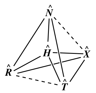
Figure 1: Commutation relations among the Hamiltonian and the symmetry operators. Commuting operators are connected with solid lines while noncommuting operators are connected with dashed lines.

Despite the nontrivial commutation property, discrete symmetry is still useful. From Eq. (15), one finds that $\hat{N}$ and $\hat{X}$ commute within the half-filling sector with $N=L/2$. Thus, inside the half-filling sector, $(\hat{H},\hat{N},\hat{T},\hat{X})$ are mutually commuting, and the Hamiltonian can be block-diagonalized as

$$\mathsf{H}_{N=L/2,k}=\mathsf{H}_{N=L/2,k,X=+1}\oplus\mathsf{H}_{N=L/2,k,X=-1}$$ (16)

for any $k$. One also finds that $\hat{R}$ and $\hat{T}$ commute within the sectors $\mathcal{S}_{N,k=0}$ and $\mathcal{S}_{N,k=L/2}$ where $\hat{T}=\hat{T}^{-1}$. Thus, the Hamiltonian in the symmetric ($k=0$) and the anti-symmetric ($k=L/2$) sectors under translation can be decomposed as

$$\mathsf{H}_{N,k}=\mathsf{H}_{N,k,R=+1}\oplus\mathsf{H}_{N,k,R=-1}$$ (17)

for any $N$. Especially, within the subspace with $(N,k)=(L/2,0)$ or $(L/2,L/2)$, all the symmetry operators mutually commute with one another. The block-diagonal structure of $\mathsf{H}$ is illustrated in Fig. 2.

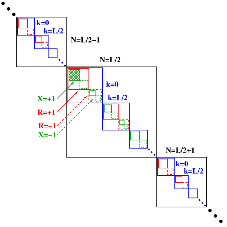
Figure 2: Block diagonal structure of the Hamiltonian matrix. The shaded area denotes the maximum symmetry sector.

III.4 Maximum Symmetry Sector

We focus on the subspace $\mathcal{S}_{N=L/2,k=0,R=+1,X=+1}$, which will be called the maximum symmetry sector (MSS). This sector corresponds to the shaded block in Fig. 2. In order to incorporate all the symmetry, we extend the concept of the equivalent class. Suppose that $|\bar{\bm{n}}\rangle$ is a RS in the half-filling sector. The symmetry operations $\hat{X}$, $\hat{R}$, and $\hat{R}\hat{X}$ map $|\bar{\bm{n}}\rangle$ to a member of other ECs represented by $|\bar{\bm{n}}_{X}\rangle$, $|\bar{\bm{n}}_{R}\rangle$, and $|\bar{\bm{n}}_{RX}\rangle$, respectively. All the involved ECs merge into a single set, which is defined as the super equivalent class (SEC). A SEC is represented by the super representative state (SRS) $|\tilde{\bm{n}}\rangle$, where

$$\tilde{\bm{n}}=\min\left[\bar{\bm{n}},\bar{\bm{n}}_{R},\bar{\bm{n}}_{X},\bar{\bm{n}}_{RX}\right].$$ (18)

A degeneracy may exist among the four numbers $\bar{\bm{n}},\bar{\bm{n}}_{R},\bar{\bm{n}}_{X}$, and $\bar{\bm{n}}_{RX}$. The number of distinct elements among the four will be denoted as the multiplicity factor $q(\tilde{\bm{n}})$ of the SEC. Then, the states

$$|\tilde{\bm{n}}\rangle_{\rm MSS}=Z(\tilde{\bm{n}})(1+\hat{X})(1+\hat{R})\left(\sum_{l=0}^{L-1}\hat{T}^{l}\right)|\tilde{\bm{n}}\rangle$$ (19)

for all SRS’s form the basis set for the MSS. The normalization factor is given by

$$Z(\tilde{\bm{n}})=\frac{\sqrt{q(\tilde{\bm{n}})}}{4}{Y(\tilde{\bm{n}})}=\frac{\sqrt{p(\tilde{\bm{n}})q(\tilde{\bm{n}})}}{4L}$$ (20)

with the function $Y$ in Eq. (7). The pseudocode to find the list of SRS’s is presented in Alg. 6. In Table 3, we list the SRS’s in the MSS for $L=8$, along with the normalization constants. The dimensionality of the MSS is listed in Table 2.

Algorithm 6 List of SRS’s for the basis set of the MSS

procedure build-SRSlistMSS($L$)

     SRSlistMSS = {}

     $\mbox{\tt basisNk}\leftarrow$ build-basisNk($L,N=L/2,k=0$)

     for ($\bar{\bm{n}}\in\mbox{\tt basisNk}$) do

         if $(\bar{\bm{n}}\leq\min[\bar{\bm{n}}_{X},\bar{\bm{n}}_{R},\bar{\bm{n}}_{RX}])$ then

              append $\bar{\bm{n}}$ to SRSlistMSS

         end if

     end for

     Return(SRSlistMSS)

end procedure

Table 3: Super representative states in the MSS for $L=8$

SRS	period $p$	multiplicity $q$	normalization $Z$
$|00001111\rangle$	8	1	$\sqrt{2}/16$
$|00010111\rangle$	8	2	$1/8$
$|00011011\rangle$	8	2	$1/8$
$|00101101\rangle$	8	1	$\sqrt{2}/16$
$|00110011\rangle$	4	1	$1/16$
$|00101011\rangle$	8	2	$1/8$
$|01010101\rangle$	2	1	$\sqrt{2}/32$

Applying the Hamiltonian to a basis state, one obtains

$$\hat{H}|\tilde{\bm{n}}\rangle_{\rm MSS}=Z(\tilde{\bm{n}})\sum_{\bm{m}}H_{\bm{m},\tilde{\bm{n}}}(1+\hat{X})(1+\hat{R})\left(\sum_{l=0}^{L-1}\hat{T}^{l}\right)|\bm{m}\rangle.$$

Thus, the Hamiltonian matrix elements in the MSS are given by

$$H^{({\rm MSS})}_{\tilde{\bm{m}}\tilde{\bm{n}}}=\frac{Z(\tilde{\bm{n}})}{Z(\tilde{\bm{m}})}\sum^{\prime}_{\bm{m}}H_{\bm{m}\tilde{\bm{n}}},$$ (21)

where the primed summation is over all states $|\bm{m}\rangle$ belonging to the same SEC as $|\tilde{\bm{m}}\rangle$. In Alg.7, we present a pseudocode to construct the matrix $\mathsf{H}_{\rm MSS}$. The explicit expression of $\mathsf{H}_{\rm MSS}$ for $L=8$ is shown in Eq. (64).

Algorithm 7 Matrix elements for $\mathsf{H}_{MSS}$

procedure build-Hmms($L$)

     SRSlistMSS $\leftarrow$ build-SRSlistMSS($L$)

     for ($\tilde{\bm{n}}\in{\tt SRSlistMSS}$) do

         $b=\mbox{find\_index\_in\_SRSlistMSS}(\tilde{\bm{n}})$

         $\mbox{\tt output}\leftarrow$ ActingH($\tilde{\bm{n}}$)

         for ($(\bm{m},h)\in{\tt output}$) do

              $\tilde{\bm{m}}=\mbox{SRS for }\bm{m}$

              $a=\mbox{find\_index\_in\_SRSlistMSS}(\tilde{\bm{m}})$

              HMMS[a,b] = HMMS[a,b] + $hZ(\tilde{\bm{n}})/Z(\tilde{\bm{m}})$

         end for

     end for

end procedure

The basis set in the other symmetry sectors can be constructed in a similar way. For each SRS $|\tilde{\bm{n}}\rangle$, one can consider a state

$$|\tilde{\bm{n}}\rangle_{w,X,R}\propto(1+X\hat{X})(1+R\hat{R})\left(\sum_{l=0}^{L-1}(w\hat{T})^{l}\right)|\tilde{\bm{n}}\rangle$$ (22)

with $X=\pm 1$, $R=\pm 1$, and $\omega=\pm 1$. It may lead to a null state or a nonvanishing state depending on $\tilde{\bm{n}}$ and $(X,R,\omega)$. The set of nonvanishing states form the basis set for $\mathcal{S}_{N=L/2,k=0,R=\pm 1,X=\pm 1}$ or ${S}_{N=L/2,k=L/2,R=\pm 1,X=\pm 1}$. The Hamiltonian matrix can also be constructed similarly, which is not shown in this paper.

IV Numerical diagonalization

We have diagonalized the Hamiltonian matrix constructed in the way explained in the previous section to solve the eigenvalue problem

$$\hat{H}|\alpha\rangle=E_{\alpha}|\alpha\rangle.$$ (23)

The numerical solution is found by diagonalizing the Hamiltonian matrix with the help of computational libraries. A computational library takes the Hamiltonian matrix $\mathsf{H}=\{H_{mn}\}$ as an input and then outputs the set of eigenvalues $\{E_{\alpha}\}$ and the unitary matrix $\mathsf{S}=\{S_{n\alpha}\}$, where $S_{n\alpha}=\langle n|\alpha\rangle$ is the $n$th component of the normalized $\alpha$th eigenstate:

$$\sum_{n}H_{mn}S_{n\alpha}=E_{\alpha}S_{m\alpha}$$ (24)

or

$$\mathsf{S}^{\dagger}\mathsf{H}\mathsf{S}={\rm diag}\{E_{\alpha}\}$$ (25)

in matrix form.

We have diagonalized the full Hamiltonian matrix $\mathsf{H}$ and the block Hamiltonians $\mathsf{H}_{N=L/2}$, $\mathsf{H}_{N=L/2,k=0}$, and $\mathsf{H}_{\rm MSS}$ for the XXZ Hamiltonian in Eq. (1) with $J=1$ and $\Delta=1/2$. The source codes are composed in C language with the Intel^® Math Kernel Library . The program was run on an Intel^® Core™i9-9900K processor. With 64-GB memory, the maximum system size accessible is $L=24$ for the MSS. Figure 3 presents the energy eigenvalue spectrum of the full Hamiltonian $\mathsf{H}$ for $L=8$ sites and of the block Hamiltonians $\mathsf{H}_{N=4}$, $\mathsf{H}_{N=4,k=0}$, and $\mathsf{H}_{\rm MMS}$. We have also measured the CPU times for the matrix construction and the diagonalization with and without eigenvectors. The CPU times are plotted in Fig. 4. Matrix diagonalization uses most of the CPU times. Roughly speaking, the CPU time scales algebraically as $D^{z}$, with the total Hilbert space dimension $D=2^{L}$ with $z\simeq 1.5$ for matrix constructions and $z\simeq 2.7$ and $2.2$ for diagonalization with and without eigenvectors, respectively.

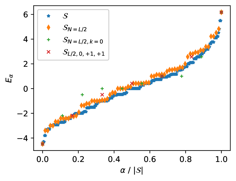
Figure 3: Energy eigenvalues are plotted as functions of the energy quantum number normalized to the Hilbert space dimension. The lattice size is $L=8$.

Figure 4: CPU times in seconds for matrix construction (open symbols with dotted lines), diagonalization without eigenvectors (filled symbols with solid lines), and diagonalization with eigenvectors (filled symbols with dashed lines). Data for the full Hamiltonian $\mathsf{H}$ and the block Hamiltonians $\mathsf{H}_{N=L/2}$, $\mathsf{H}_{N=L/2,k=0}$, and $\mathsf{H}_{\rm MMS}$ are marked with circular, square, diamond, and triangular symbols, respectively.

V Numerical Study of Quantum Thermalization

As an application of the numerical technique, we investigate the quantum thermalization of the XXZ model with nearest and next-nearest neighbor interactions. As mentioned in Section I, quantum systems which thermalize are believed to obey the ETH, which assumes that matrix elements $O_{\alpha\gamma}=\langle\alpha|\hat{O}|\gamma\rangle$ of a local observable $\hat{O}$ in the Hamiltonian eigenstates basis take the form Srednicki (1996, 1999)

$$O_{\alpha\gamma}=O(E_{\alpha\gamma})\delta_{\alpha\gamma}+e^{-S(E_{\alpha\gamma})/2k_{B}}f_{O}(E_{\alpha\gamma},\omega_{\alpha\gamma})R_{\alpha\gamma},$$ (26)

where $S$ is the thermodynamic entropy, $O$ and $f_{O}$ are smooth functions of $E_{\alpha\gamma}=(E_{\alpha}+E_{\gamma})/2$ and $\omega_{\alpha\gamma}=(E_{\alpha}-E_{\gamma})/\hbar$, and $R_{\alpha\gamma}$ are random matrix elements. The Boltzmann constant $k_{B}$ and the Planck constant $\hbar$ will be set to unity. The ETH guarantees that the quantum mechanical expectation value is equal to the microcanonical ensemble average. The ETH is believed to hold for generic nonintegrable quantum systems D’Alessio et al. (2016).

We investigate the XXZ spin chain Hamiltonian with nearest and next-nearest neighbor interactions. The XXZ Hamiltonian in Eq. (1) with only nearest neighbor interactions is a representative example of a nonthermal integrable system Rigol (2009). It can be made nonintegrable by adding the next-nearest neighbor couplings Yoshizawa et al. (2018). We consider the Hamiltonian

$$\hat{H}=\frac{1}{1+\lambda}\left(\hat{H}_{nn}+\lambda\hat{H}_{nnn}\right),$$ (27)

where $\hat{H}_{nn}$ is equal to the Hamiltonian in Eq. (1) and $\hat{H}_{nnn}$ denotes the same type of Hamiltonian whose interaction and hopping ranges are modified to the next-nearest neighbors. With nonzero $\lambda$ and $\Delta$, the Hamiltonian is known to obey the ETH Yoshizawa et al. (2018).

Even in the presence of the next-nearest neighbor interactions, one can use the same method to construct the basis set and the Hamiltonian matrix. One needs to modify Alg. 1 in order to include the additional interaction terms only. In numerical calculations hereafter, we fix the values of $J$ to $1$, $\lambda$ to $1$, and $\Delta$ to $1/2$. In general, one should be able to handle any subspace of the whole Hilbert space. If the subspace is intractable in a brute-force way, one needs to decompose the subspace into symmetry sectors, as explained in Section III. The MSS has the largest dimensionality among all the symmetry sectors and is the hardest obstacle in numerical studies. Thus, we mainly focus on the MSS in the numerical demonstration.

V.1 Energy Eigenstate Expectation Value

The ETH suggests that the energy eigenstate expectation value of a local observable $\hat{O}$ should depend only on the energy eigenvalue in the thermodynamic limit. We test the hypothesis for two observables: the zero momentum distribution function

$$\hat{A}=\frac{1}{L}\sum_{l,m=0}^{L-1}\hat{b}_{l}^{\dagger}\hat{b}_{m}=\frac{1}{L}\sum_{l,m}\hat{\sigma}_{l}^{+}\hat{\sigma}_{m}^{-}$$ (28)

and the nearest neighbor interaction energy density

$$\hat{B}=\frac{1}{L}\sum_{l}\hat{n}\hat{n}_{l+1}=\frac{1}{L}\sum_{l}\frac{\hat{\sigma}_{l}^{z}+1}{2}\frac{\hat{\sigma}_{l+1}^{z}+1}{2}.$$ (29)

These operators commute with the symmetry operators $\hat{N}$, $\hat{T}$, $\hat{R}$, and $\hat{X}$ within the MSS. Thus, the matrix representations $\mathsf{A}$ and $\mathsf{B}$ in the basis set $\{|\tilde{\bm{n}}\rangle_{\rm MSS}\}$ can be constructed by using the algorithm explained in Alg. 7. One needs to provide the subroutine that generates the output states by using the action of the observable operator $\hat{O}$ in a similar way as shown in Alg. 1. The energy eigenstate expectation values of $\hat{O}$ are given by

$$O_{\alpha}=\langle\alpha|\hat{O}|\alpha\rangle=\sum_{m}S_{m\alpha}^{*}\left(\sum_{n}O_{mn}S_{n\alpha}\right),$$ (30)

where $S_{n\alpha}$ is the column vector for the $\alpha$-th eigenstate of the Hamiltonian (see Eqs. (24) and (25)).

We plot the eigenstate expectation values in the MSS as functions of the energy eigenvalues per site in Fig. 5. For a given value of $E_{\alpha}/L$, the expectation values spread over a finite range. One can see that the fluctuations become weaker and weaker as $L$ grows. The ETH in Eq. (26) predicts that the fluctuations should scale as $e^{-S(E)}$, which vanishes exponentially as $L$ increases. The numerical data are consistent with the ETH prediction. For quantitative analysis of the fluctuations, we refer the readers to Ref. LeBlond et al. (2019).

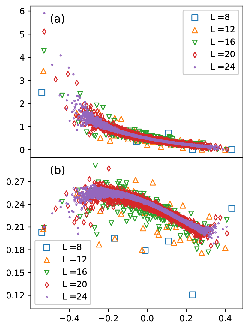
Figure 5: Energy eigenstate expectation values of (a) $\hat{A}$ and (b) $\hat{B}$ are plotted as functions of the energy eigenvalue.

V.2 Energy-Temperature Relation

If the energy eigenstate expectation value depends only on the energy eigenvalue, the expectation value becomes the same as the microcanonical ensemble average D’Alessio et al. (2016). Due to the ensemble equivalence, the expectation value is then equal to the canonical ensemble average:

$$O_{\alpha}={\rm Tr}\hat{\rho}_{eq}(\beta)\hat{O},$$ (31)

where $\hat{\rho}_{eq}(\beta)=e^{-\beta\hat{H}}/Z$ is the density matrix of the canonical ensemble with the partition function $Z={\rm Tr}e^{-\beta\hat{H}}$ and the inverse temperature $\beta=1/T$. Consequently, each energy eigenstate $|\alpha\rangle$ with the energy eigenvalue $E_{\alpha}$ is assigned to an inverse temperature through the relation

$$E_{\alpha}={\rm Tr}\hat{\rho}_{eq}(\beta)\hat{H}=\frac{\sum_{\gamma}E_{\gamma}e^{-\beta E_{\gamma}}}{\sum_{\gamma}e^{-\beta E_{\gamma}}}.$$ (32)

The energy is an extensive quantity so that the Boltzmann factors $e^{-\beta E_{\alpha}}$ are distributed widely. In order to reduce possible numerical errors in evaluating the summation over such quantities, we recommend that the Kahan algorithm or the compensation algorithm be used Kahan (1965). We evaluate numerically the mean energy as a function of $\beta$ in the MSS for various values of $L$ (Fig. 6).

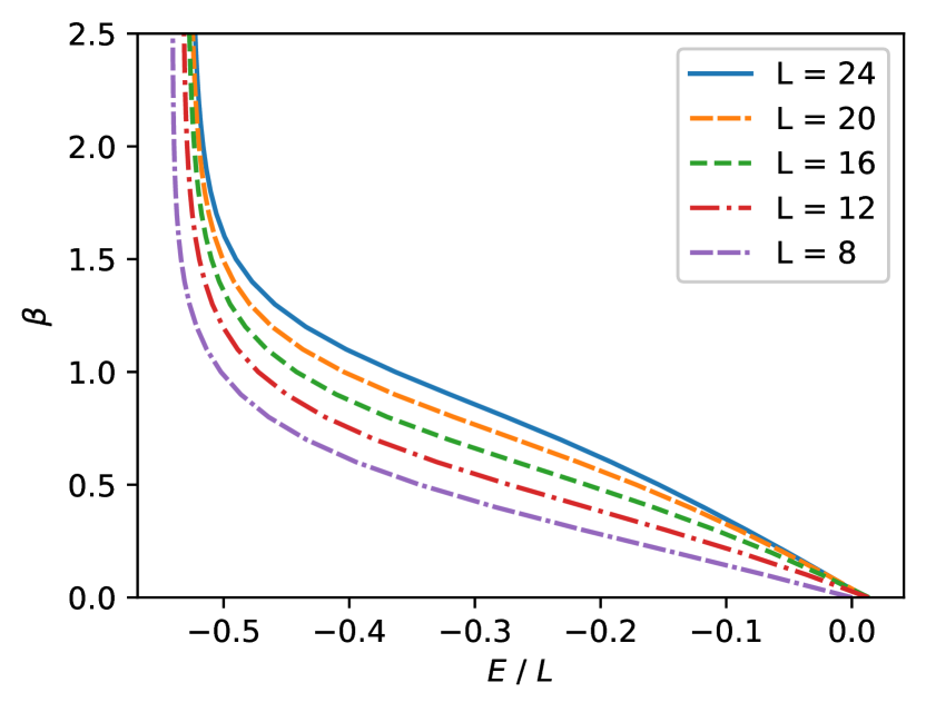
Figure 6: Energy density $E/L$ versus inverse temperature $\beta$ according to Eq. (32).

V.3 Time Evolution

Suppose that the system is in an initial state

$$|\psi_{0}\rangle=\sum_{n}a_{\bm{n}}|\bm{n}\rangle$$ (33)

at time $t=0$. Following the Schrödinger equation, the system evolves into the state

$$|\psi(t)\rangle=\hat{U}(t)|\psi_{0}\rangle$$ (34)

with the time evolution operator

$$\hat{U}(t)=\exp[-i\hat{H}t].$$ (35)

We are interested in the time-dependent probability amplitudes $\{a_{\bm{n}}(t)\}$ with which the state

$$|\psi(t)\rangle=\sum_{\bm{n}}a_{\bm{n}}(t)|\bm{n}\rangle$$ (36)

solves the Schrödinger equation.

When the whole eigenspectrum of the Hamiltonian operator is available, decomposing the initial state in terms of the energy eigenstates $\{|\alpha\rangle\}$,

$$|\psi_{0}\rangle=\sum_{\alpha}C_{\alpha}|\alpha\rangle,$$ (37)

with

$$C_{\alpha}=\langle\alpha|\psi_{0}\rangle=\sum_{\bm{n}}\langle\alpha|\bm{n}\rangle\langle\bm{n}|\psi_{0}\rangle=\sum_{\bm{n}}S^{*}_{{\bm{n}}\alpha}a_{\bm{n}},$$ (38)

is convenient. Note that $\mathsf{S}=\{S_{{\bm{n}}\alpha}\}$ is the unitary matrix diagonalizing $\mathsf{H}$ (see Eq. (25)). Inserting Eq. (37) into Eq. (34), one obtains

$$a_{\bm{n}}(t)=\sum_{\alpha}S_{{\bm{n}}\alpha}\left(C_{\alpha}e^{-iE_{\alpha}t}\right).$$ (39)

Thus, the state at arbitrary time $t$ can be found by performing the matrix-vector multiplication in Eqs. (38) and (39). If the initial state $|\psi_{0}\rangle$ belongs to a specific symmetry sector, knowledge of the eigenvalues and the eigenvectors within the sector is sufficient.

We demonstrate the time evolution starting from the initial state

$$|\psi_{0}\rangle=\frac{1}{\sqrt{2}}(|0101\cdots\rangle+|1010\cdots\rangle).$$ (40)

It belongs to the MSS with SRS $|\tilde{\bm{n}}\rangle=|0101\cdots\rangle$. It is decomposed into a linear superposition of the energy eigenstates in the MSS; then, the probability amplitudes at time $t$ are obtained from Eq. (39). In Fig. 7, we present the time-dependent expectation values of $\hat{A}$ and $\hat{B}$. After an initial transient region, both quantities relax into stationary values with fluctuations. The amplitude of the fluctuations decreases as $L$ increases for both quantities. An approach to a stationary state is guaranteed when the initial state overlaps a large enough number of energy eigenstates Reimann (2008); Short (2011).

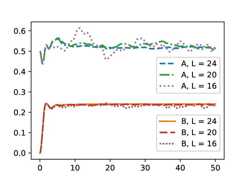
Figure 7: Time-dependent expectation values of $\hat{A}$ and $\hat{B}$ for systems with $L=16,20$, and $24$.

When the whole set of eigenvalues and the eigenvectors is not available, the Lie-Trotter-Suzuki (LTS) decomposition method is useful Suzuki (1985). The Hamiltonian is a sum of local operators that do not commute with one another. Rearranging those local operators, one can decompose the Hamiltonian into multiple partial Hamiltonians in such a way that each partial Hamiltonian should consist of a set of mutually commuting local operators. For clarity, we explain the method with the XXZ Hamiltonian in Eq. (1) with only the nearest neighbor interaction (see Eq. (52) for the case with the next-nearest neighbor interactions). The Hamiltonian can be written as

$$\hat{H}=\sum_{l=0}^{L-1}\hat{h}_{l,l+1},$$ (41)

where

$$\hat{h}_{l,m}=-\hat{\sigma}_{l}^{+}\hat{\sigma}_{m}^{-}-\hat{\sigma}_{l}^{-}\hat{\sigma}_{m}^{+}-\frac{\Delta}{2}\hat{\sigma}_{l}^{z}\hat{\sigma}_{m}^{z}$$ (42)

is the XXZ coupling between two spins at sites $l$ and $m$. The Hamiltonian can be written as

$$\hat{H}=\hat{H}_{0}+\hat{H}_{1}$$ (43)

with $\hat{H}_{0}=\sum_{l=0}^{L/2-1}\hat{h}_{2l,2l+1}$ and $\hat{H}_{1}=\sum_{l=0}^{L/2-1}\hat{h}_{2l+1,2l+2}$. Checking that $\hat{H}_{0}$ and $\hat{H}_{1}$ are the sum of mutually commuting operators, respectively, is easy.

The LTS method is based on the Baker-Campbell-Hausdorff formula

$$e^{\delta(\hat{A}+\hat{B})}=e^{\delta\hat{A}}e^{\delta\hat{B}}e^{-\frac{\delta^{2}}{2}[\hat{A},\hat{B}]}\cdots$$ (44)

Applying it to $\hat{U}(t=\epsilon)=e^{-i\epsilon(\hat{H}_{0}+\hat{H}_{1})}$, one obtains $\hat{U}(\epsilon)=\hat{U}_{LTS}(\epsilon)+O(\epsilon^{2})$ with the approximate time evolution operator

$$\hat{U}_{LTS}(\epsilon)=e^{-i\epsilon\hat{H}_{0}}e^{-i\epsilon\hat{H}_{1}}.$$ (45)

Due to the commutation property, $\hat{U}_{LTS}(\epsilon)$ takes the product form

$$\hat{U}_{LTS}(\epsilon)=\left[\prod_{l=0}^{L/2-1}\hat{u}_{2l,2l+1}\right]\left[\prod_{l=0}^{L/2-1}\hat{u}_{2l+1,2l+2}\right],$$ (46)

where

$$\hat{u}_{l,m}\equiv e^{-i\epsilon\hat{h}_{l,m}}$$ (47)

acts only on two sites $l$ and $m$. The true time evolution operator $\hat{U}(\epsilon)$ rotates all spins simultaneously. On the other hand, $\hat{U}_{LTS}(\epsilon)$ rotates pairs of spins successively, which is easily done computationally. The two-spin rotation operator $\hat{u}_{l,m}$ is represented by the $4\times 4$ matrix

$$\mathsf{u}=\begin{pmatrix}e^{i\Delta\epsilon/2}&0&0&0\\ 0&e^{-i\Delta\epsilon/2}\cos\epsilon&ie^{-i\Delta\epsilon/2}\sin{\epsilon}&0\\ 0&ie^{-i\Delta\epsilon/2}\sin\epsilon&e^{-i\Delta\epsilon/2}\cos{\epsilon}&0\\ 0&0&0&e^{i\Delta\epsilon/2}\end{pmatrix}$$ (48)

with the basis set

$$\{|0\rangle_{l}\otimes|0\rangle_{m},|0\rangle_{l}\otimes|1\rangle_{m},|1\rangle_{l}\otimes|0\rangle_{m},|1\rangle_{l}\otimes|1\rangle_{m}\}.$$

The pseudocode for the two-spin rotation is presented in Alg. 8.

Algorithm 8 Two-spin rotation $|\psi^{\prime}\rangle=\hat{u}_{l,m}|\psi\rangle$ for $|\psi\rangle=\sum_{\bm{n}}a_{\bm{n}}|{\bm{n}}\rangle$

procedure Acting_u($|\psi\rangle,L,l,m$)

     $a_{\bm{n}}^{\prime}=0$ for all $\bm{n}$

     for (${\bm{n}}=0$ to $2^{L}-1$) do

         $n_{l}=l\mbox{th bit of }n$ ; $n_{m}=m\mbox{th bit of }{\bm{n}}$

         if $(n_{l}=n_{m})$ then

              $a^{\prime}_{\bm{n}}=a^{\prime}_{\bm{n}}+a_{\bm{n}}e^{i\Delta\epsilon/2}$

         else

              $a^{\prime}_{\bm{n}}=a^{\prime}_{\bm{n}}+a_{\bm{n}}e^{-i\Delta\epsilon}\cos\epsilon$

              ${\bm{m}}=\mbox{bit\_flip}(\bm{n},l,m)$

              $a^{\prime}_{{\bm{m}}}=a^{\prime}_{{\bm{m}}}+a_{\bm{n}}ie^{-i\Delta\epsilon/2}\sin\epsilon$

         end if

     end for

     Return( $|\psi^{\prime}\rangle=\sum_{\bm{n}}a^{\prime}_{\bm{n}}|{\bm{n}}\rangle$ )

end procedure

A few remarks are in order: (i) One may consider the approximation $\hat{U}(\epsilon)\simeq 1-i\epsilon\hat{H}+O(\epsilon^{2})$, which is analogous to the Euler method for ordinary differential equations. Such an approximation is not recommended because it breaks unitarity of the time evolution operator Askar and Cakmak (1978). (ii) $\hat{U}_{LTS}(\epsilon)$ is unitary, conserves the particle number, and commutes with $\hat{X}$ as the original time evolution operator $\hat{U}$. Unfortunately, however, it does not commute with $\hat{T}$ and $\hat{R}$. If the symmetry property is important, one should use the symmetrized form $\hat{U}_{LTS,s}(\epsilon)=(e^{-i\epsilon\hat{H}_{0}}e^{-i\epsilon\hat{H}_{1}}+e^{-i\epsilon\hat{H}_{1}}e^{-i\epsilon\hat{H}_{0}})/2$. (iii) The wave function after time $t$ is obtained by applying the infinitesimal time evolution operator $t/\epsilon$ times, which leads to a numerical error of $O(t\epsilon)$. If one uses the higher-order expansion formula Suzuki (1985)

$$e^{\delta(\hat{A}+\hat{B})}=e^{\frac{\delta}{2}\hat{A}}e^{\delta\hat{B}}e^{\frac{\delta}{2}\hat{A}}+O(\delta^{3})\ ,$$ (49)

one can reduce the numerical error. Thus, using the higher order approximation

$$\hat{U}_{LTS}(\epsilon)=e^{-i\epsilon\hat{H}_{0}/2}e^{-i\epsilon\hat{H}_{1}}e^{-i\epsilon\hat{H}_{0}/2}\ ,$$ (50)

whose overall numerical error scales as $O(t\epsilon^{2})$, would be wise.

When the Hamiltonian includes next-nearest neighbor interactions as in Eq. (27), the Hamiltonian may be decomposed as

$$\hat{H}=\hat{H}_{0}+\left(\hat{H}_{1}+\left(\hat{H}_{2}+\hat{H}_{3}\right)\right)$$ (51)

with $\hat{H}_{2}=\sum_{l=0}^{L/4-1}(\hat{h}_{4l,4l+2}+\hat{h}_{4l+1,4l+3})$ and $\hat{H}_{3}=\sum_{l=0}^{L/4-1}(\hat{h}_{4l+2,4l+4}+\hat{h}_{4l+3,4l+5})$. Applying Eq. (50) successively Noh et al. (2019), one find that $\hat{U}(\epsilon)=\hat{U}_{LTS}(\epsilon)+O(\epsilon^{3})$, where

$$\begin{split}\hat{U}_{LTS}(\epsilon)=&e^{-i\epsilon\hat{H}_{0}/2}e^{-i\epsilon\hat{H}_{1}/2}e^{-i\epsilon\hat{H}_{2}/2}e^{-i\epsilon\hat{H}_{3}}\\ &\times e^{-i\epsilon\hat{H}_{2}/2}e^{-i\epsilon\hat{H}_{1}/2}e^{-i\epsilon\hat{H}_{0}/2}.\end{split}$$ (52)

We compare in Fig. 8 the time evolutions of the expectation values of $\hat{A}$ and $\hat{B}$ calculated from the exact wave function in Eq. (39) and from the approximate decomposition method in Eq. (52). The lattice size is $L=14$, and the initial state is $|\psi_{0}\rangle$ in Eq. (40). As $t$ increases, the approximate solution deviates from the exact solution. The error decreases as $\epsilon$ becomes smaller. Because the infinitesimal time evolution operator has an error of $O(\epsilon^{3})$, the numerical error at finite $t$ scales as $O(t\epsilon^{2})$.

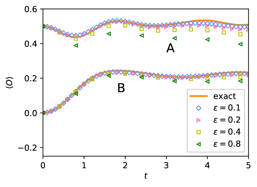
Figure 8: Time evolution of the expectation values of $\hat{O}=\hat{A}$ and $\hat{B}$ calculated by using the exact time-dependent wave function and the approximate time-evolution operator in Eq. (52) with $\epsilon=0.1,\cdots,0.8$. The lattice size is $L=14$.

V.4 Entanglement Entropy

The entanglement is a characteristic feature of a quantum mechanical system Amico et al. (2008); Kim and Huse (2013); Vidmar et al. (2018). It measures the extent to which a part $S_{1}$ of a system and its complement $S_{2}=S_{1}^{c}$ are interwound with each other. Let $\{|\bm{r}\rangle\}$ and $\{|\bm{l}\rangle\}$ be the basis sets of the subsystems $S_{1}$ and $S_{2}$ whose Hilbert space dimensions are $D_{1}$ and $D_{2}$, respectively. Then, a state vector can be written as

$$|\psi\rangle=\sum_{\bm{l},\bm{r}}\psi_{\bm{l}\bm{r}}|\bm{l}\rangle\otimes|\bm{r}\rangle.$$ (53)

If the probability amplitudes are factorized as $\psi_{\bm{l}\bm{r}}=\phi_{\bm{l}}\varphi_{\bm{r}}$, the state vector is unentangled and is given by the direct product $|\psi\rangle=\left(\sum_{\bm{l}}\phi_{\bm{l}}|\bm{l}\rangle\right)\otimes\left(\sum_{\bm{r}}\varphi_{\bm{r}}|\bm{r}\rangle\right)$. Otherwise, it is entangled. The entanglement can be quantified by using the von Neumann entropy

$$S_{E}=-{\rm Tr}_{1}\hat{\rho}_{1}\ln\hat{\rho}_{1}$$ (54)

of the reduced density matrix

$$\hat{\rho}_{1}={\rm Tr}_{2}|\psi\rangle\langle\psi|=\sum_{\bm{l}}\psi_{\bm{l}\bm{r}}\psi_{\bm{l}\bm{r}^{\prime}}^{*}|\bm{r}\rangle\langle\bm{r}^{\prime}|$$ (55)

for the subsystem $S_{1}$. In terms of the eigenvalues $\{\lambda^{1}_{i}\}$ of $\hat{\rho}_{1}$, the entanglement entropy is given by

$$S_{E}=-\sum_{i=1}^{D_{1}}\lambda^{1}_{i}\ln\lambda^{1}_{i}\ .$$ (56)

The singular value decomposition (SVD) is extremely useful in calculating the reduced density matrix and the entanglement entropy. The probability amplitude $\psi_{\bm{lr}}$ can be regarded as an element of the $D_{2}\times D_{1}$ matrix $\mathsf{\Psi}$. Any matrix with complex elements can be written in a product form Golub and Van Loan (1996)

$$\mathsf{\Psi}=\mathsf{U}\mathsf{\Sigma}\mathsf{V}^{\dagger},$$ (57)

with a $D_{2}\times D_{1}$ rectangular matrix $\mathsf{\Sigma}$ and a unitary matrix $\mathsf{U}~{}(\mathsf{V})$ of size $D_{\rm 2}\times D_{\rm 2}~{}(D_{\rm 1}\times D_{\rm 1})$. The off-diagonal elements of the rectangular matrix $\Sigma$ are zero, and the diagonal elements $\{\Sigma_{1},\cdots,\Sigma_{\min[D_{\rm 2},D_{\rm 1}]}\}$ are real and nonnegative Golub and Van Loan (1996). The diagonal elements are called the singular values. The reduced density matrix for the subsystem $S_{1}$ is given by

$$\mathsf{\rho}_{1}=\mathsf{\Psi}^{\dagger}\mathsf{\Psi}=\mathsf{V}(\mathsf{\Sigma}^{\dagger}\mathsf{\Sigma})\mathsf{V}^{\dagger},$$ (58)

which is the similarity transformation of the $(D_{1}\times D_{1})$ diagonal matrix $\mathsf{\Sigma}^{\dagger}\mathsf{\Sigma}={\rm diag}[\Sigma_{1}^{2},\cdots,\Sigma_{\min[D_{1},D_{2}]}^{2},0,\cdots,0]$. Thus, the entanglement entropy is given by

$$S_{E}=-\sum_{i=1}^{\min[D_{1},D_{2}]}(\Sigma_{i})^{2}\ln(\Sigma_{i})^{2}.$$ (59)

The reduced density matrix for the alternative subsystem $S_{2}$ is given by $\rho_{2}=\mathsf{\Psi}\mathsf{\Psi}^{\dagger}=\mathsf{U(\Sigma\Sigma}^{\dagger})\mathsf{U}^{\dagger}$. It shares the same nonzero eigenvalues with $\rho_{1}$. Thus, the two subsystems $S_{1}$ and $S_{2}$ have the same von Neumann entropy and yield the same entanglement entropy.

Using the SVD method, one can calculate the entanglement entropy of the one-dimensional system efficiently. Consider a partition of the one-dimensional lattice of $L$ sites into two subsets: $S_{1}$ for the rightmost $L_{\rm 1}$ sites at $l=0,1,\cdots,L_{1}-1$ and $S_{2}$ for $L_{2}=(L-L_{1})$ sites at $l=L_{1},\cdots,L-1$. A basis state $|\bm{n}\rangle$ with $0\leq\bm{n}<2^{L}$ for the whole system can be written as a product state $|\bm{l}\rangle\otimes|\bm{r}\rangle$, where $0\leq\bm{l}<D_{2}=2^{L_{2}}$ and $0\leq\bm{r}<D_{1}=2^{L_{1}}$ are related to $\bm{n}$ through

$$\bm{n}=2^{L_{1}}\bm{l}+\bm{r}.$$ (60)

That is, $\bm{r}$ and $\bm{l}$ are the remainder and the quotient in the integer division of $\bm{n}$ by $D_{1}=2^{L_{1}}$. Accordingly, any state $|\psi\rangle=\sum_{\bm{n}}a_{\bm{n}}|\bm{n}\rangle$ can be written in the form of Eq. (53) by identifying $\psi_{\bm{lr}}=a_{\bm{n}}$. If one is interested only in the entanglement entropy, calculating the singular values while neglecting the unitary matrices $\mathsf{U}$ and $\mathsf{V}$ will suffice. A pseudocode for the entanglement entropy is presented in Alg. 9. The crucial part is the subroutine to perform the SVD, which is found in standard numerical libraries.

Algorithm 9 Entanglement entropy for a state $|\psi\rangle=\sum_{\bm{n}}a_{\bm{n}}|{\bm{n}}\rangle$

procedure EntanglementEntropy($|\psi\rangle,L,L_{1},L_{2}$)

     for (${\bm{n}}=0$ to $2^{L}-1$) do

         $\bm{r}=\mbox{remainder of }\bm{n}/2^{L_{1}}$; $\bm{l}=\mbox{quotient of }\bm{n}/2^{L_{1}}$

         $\psi_{\bm{l}\bm{r}}=a_{\bm{n}}$

     end for

     $(\mathsf{\Sigma,U,V})\leftarrow\mbox{{SVD}}(\mathsf{\Psi},2^{L_{2}},2^{L_{1}})$

     ${\tt Entropy}=-\sum_{i}(\Sigma_{i})^{2}\ln(\Sigma_{i})^{2}$

     Return(Entropy)

end procedure

We have calculated the entanglement entropy for the energy eigenstate of the XXZ Hamiltonian in Eq. (27). For each $L$, we have chosen the eigenstate $|\alpha\rangle$ in the MSS whose energy density $E_{\alpha}/L$ is closest to $-0.2$ or $0$. The entanglement entropy $S_{E}(L_{1})$ as a function of the subsystem size $L_{1}$ is shown in Fig. 9. The von Neumann entropy of the subsystems $S_{1}$ and $S_{2}$ are the same. Thus, $S_{E}(L_{1})=S_{E}(L-L_{1})$ and $S_{E}(0)=S_{E}(L)=0$. For $0\ll L_{1}\ll L/2$, the entanglement entropy is proportional to $L_{1}$, obeying the volume law Garrison and Grover (2018). Numerical estimates for the slope are $s=0.60$ and $s=0.69$ for the energy densities $E_{\alpha}/L=-0.2$ and $0.0$, respectively. For quantum systems that thermalize, the slope is equal to the thermodynamic entropy density $s=S/L$ Garrison and Grover (2018). The system with $E_{\alpha}/L=0.0$ is in an infinite temperature state (see Fig. 6) where the thermodynamic entropy density is $s=\ln 2$. The numerical result for the slope $s=0.69$ for the states with $E_{\alpha}/L=0.0$ is consistent with the entropy density at infinite temperature.

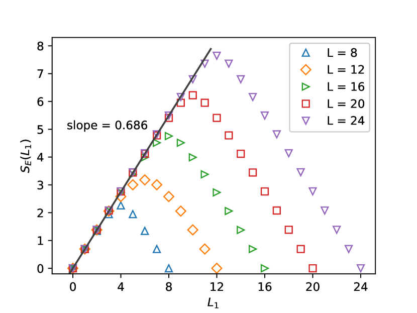
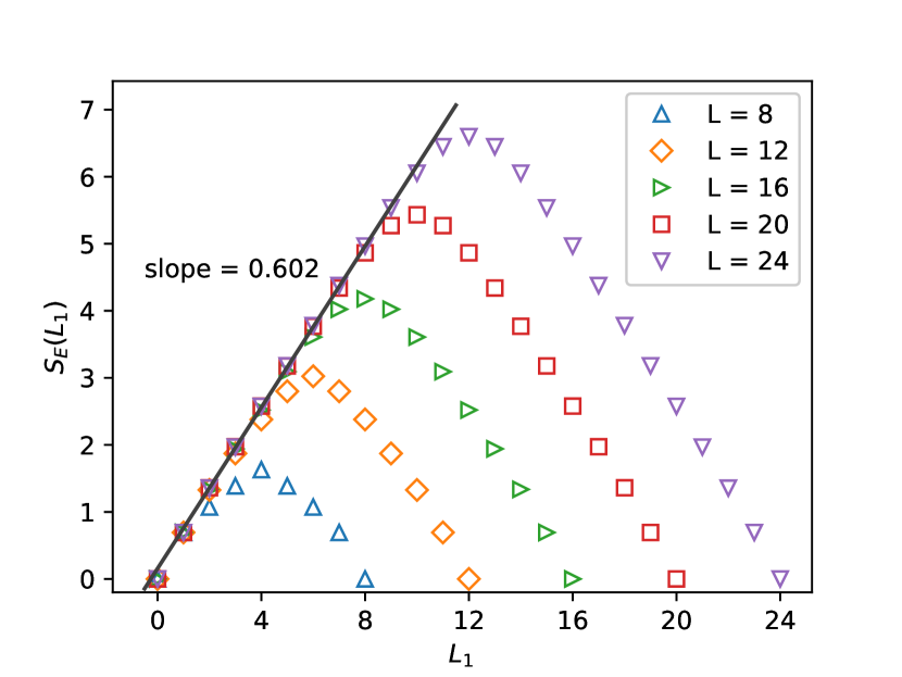
Figure 9: Entanglement entropy $S_{E}(L_{R})$ of the energy eigenstates whose energy densities are closest to $0$ and $-0.2$.

We also study the time evolution of the entanglement entropy starting from the initial state $|\psi_{0}\rangle$ in Eq. (40), which is not the energy eigenstate. Figure 10 shows the numerical results obtained for system with $L=24$. The initial state has the reduced density matrix

$$\hat{\rho}_{1}=\frac{1}{2}\left(|\overbrace{01\cdots}^{L_{1}}\rangle\langle\overbrace{01\cdots}^{L_{1}}|+|\overbrace{10\cdots}^{L_{1}}\rangle\langle\overbrace{10\cdots}^{L_{1}}|\right),$$

whose von Neumann entropy is $\ln 2$ for $L_{1}\neq 0,L$. The plateau at $t=0$ explains the initial entanglement entropy. Linear regions appear near $L_{1}=0$ and $L$ at $t>0$, the size of which grows in time. Eventually, the entanglement entropy converges to a stationary distribution that satisfies the volume law Kim and Huse (2013).

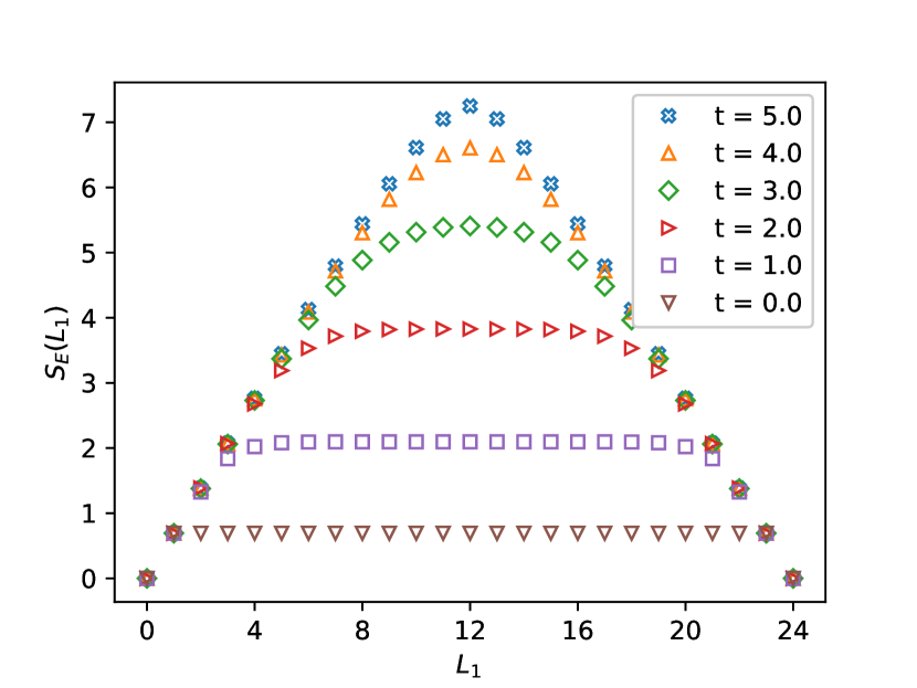
Figure 10: Time evolution of the entanglement entropy for the system with $L=24$.

VI Summary

In this paper, we present a thorough review of a numerical method to diagonalize the quantum mechanical Hamiltonian. The method is applicable to systems with finite Hilbert space dimensionality. In the presence of particle number conservation and translational invariance, the Hamiltonian matrix can be broken up into symmetry sectors specified with the eigenvalues of the number operator and the shift operator. One can further make use of discrete symmetry such as the particle-hole symmetry and the spatial inversion symmetry to reduce the matrix size effectively.

As an application of the numerical method, we studied the XXZ model Hamiltonian with nearest and next-nearest neighbor interactions. We present various numerical results in the maximum symmetry sector up to the lattice size $L=24$. The energy eigenvalues (Fig. 3) and the CPU time for the diagonalization (Fig. 4) are presented in Section IV. The XXZ Hamiltonian is a prototypical model for the study of quantum thermalization. We also present the expectation values of observables (Fig. 5), the inverse temperature (Fig. 6), the relaxation dynamics, and the entanglement entropy (Fig. 9) in Section V with the numerical methods for those quantities. We hope that our review will be helpful to those who are interested in the numerical study of the quantum thermalization of isolated quantum systems.

Appendix

In this Appendix, we present the explicit representation of the Hamiltonian matrix for systems with small $L$. When $L=4$, the Hamiltonian in Eq. (1) can be represented by a $16\times 16$ matrix in the basis set $\{|\bm{0}\rangle,\cdots,|\bm{15}\rangle\}$, given by

$$\mathsf{H}=\setcounter{MaxMatrixCols}{16}\begin{pmatrix}-2\Delta&0&0&0&0&0&0&0&0&0&0&0&0&0&0&0\\ 0&0&-1&0&0&0&0&0&-1&0&0&0&0&0&0&0\\ 0&-1&0&0&-1&0&0&0&0&0&0&0&0&0&0&0\\ 0&0&0&0&0&-1&0&0&0&0&-1&0&0&0&0&0\\ 0&0&-1&0&0&0&0&0&-1&0&0&0&0&0&0&0\\ 0&0&0&-1&0&2\Delta&-1&0&0&-1&0&0&-1&0&0&0\\ 0&0&0&0&0&-1&0&0&0&0&-1&0&0&0&0&0\\ 0&0&0&0&0&0&0&0&0&0&0&-1&0&0&-1&0\\ 0&-1&0&0&-1&0&0&0&0&0&0&0&0&0&0&0\\ 0&0&0&0&0&-1&0&0&0&0&-1&0&0&0&0&0\\ 0&0&0&-1&0&0&-1&0&0&-1&2\Delta&0&-1&0&0&0\\ 0&0&0&0&0&0&0&-1&0&0&0&0&0&-1&0&0\\ 0&0&0&0&0&-1&0&0&0&0&-1&0&0&0&0&0\\ 0&0&0&0&0&0&0&0&0&0&0&-1&0&0&-1&0\\ 0&0&0&0&0&0&0&-1&0&0&0&0&0&-1&0&0\\ 0&0&0&0&0&0&0&0&0&0&0&0&0&0&0&-2\Delta\end{pmatrix}$$ (61)

Using particle number conservation, we can write the Hamiltonian matrix in Eq. (61) in block-diagonal form as

$$\mathsf{H}=\begin{pmatrix}\boxed{\begin{matrix}-2\Delta\end{matrix}}&&&&\\ &\boxed{\begin{matrix}0&-1&0&-1\\ -1&0&-1&0\\ 0&-1&0&-1\\ -1&0&-1&0\\ \end{matrix}}&&&\\ &&\boxed{\begin{matrix}0&-1&0&0&-1&0\\ -1&2\Delta&-1&-1&0&-1\\ 0&-1&0&0&-1&0\\ 0&-1&0&0&-1&0\\ -1&0&-1&-1&2\Delta&-1\\ 0&-1&0&0&-1&0\end{matrix}}&&\\ &&&\boxed{\begin{matrix}0&-1&0&-1\\ -1&0&-1&0\\ 0&-1&0&-1\\ -1&0&-1&0\end{matrix}}&\\ &&&&\boxed{\begin{matrix}-2\Delta\end{matrix}}\end{pmatrix}.$$ (62)

Each block corresponds to an $N$-particle sector with $N=0~{}(\mbox{top}),1,2,3,4~{}(\mbox{bottom})$. Using the translational symmetry, we can further block-diagonalize $\mathsf{H}_{N}$ by using the wave-number quantum number $k=0,\cdots,L-1$. The block-diagonal form of $\mathsf{H}_{2}$ in the $N=2$ particle sector is given by

$$\mathsf{H}_{2}=\begin{pmatrix}\boxed{\begin{matrix}0&-2\sqrt{2}\\ -2\sqrt{2}&2\Delta\end{matrix}}&&&\\ &\boxed{\begin{matrix}0\end{matrix}}&&\\ &&\boxed{\begin{matrix}0&0\\ 0&2\Delta\end{matrix}}&\\ &&&\boxed{\begin{matrix}0\end{matrix}}\end{pmatrix}$$ (63)

where the blocks correspond to $\mathsf{H}_{2,0}$ (top), $\mathsf{H}_{2,1}$, $\mathsf{H}_{2,2}$, and $\mathsf{H}_{2,3}$ (bottom). The Hamiltonian matrix in the MSS for $L=8$ is given by

$$\mathsf{H}_{\rm MMS}=\begin{pmatrix}-2\Delta&-\sqrt{2}&0&0&0&0&0\\ -\sqrt{2}&0&-2&-\sqrt{2}&0&0&0\\ 0&-2&0&0&0&-2&0\\ 0&-\sqrt{2}&0&2\Delta&0&-2\sqrt{2}&0\\ 0&0&0&0&0&-2&0\\ 0&0&-2&-2\sqrt{2}&-2&2\Delta&-2\sqrt{2}\\ 0&0&0&0&0&-2\sqrt{2}&4\Delta\end{pmatrix}$$ (64)

References

- D’Alessio et al. (2016) Luca D’Alessio, Yariv Kafri, Anatoli Polkovnikov, and Marcos Rigol, “From quantum chaos and eigenstate thermalization to statistical mechanics and thermodynamics,” Adv. Phys. 65, 239–362 (2016).
- Deutsch (2018) Joshua M Deutsch, “Eigenstate thermalization hypothesis,” Rep. Prog. Phys. 81, 082001–17 (2018).
- Srednicki (1996) Mark Srednicki, “Thermal fluctuations in quantized chaotic systems,” J. Phys. A 29, L75–L79 (1996).
- Srednicki (1999) Mark Srednicki, “The approach to thermal equilibrium in quantized chaotic systems,” J. Phys. A 32, 1163–1175 (1999).
- Rigol et al. (2008) Marcos Rigol, Vanja Dunjko, and Maxim Olshanii, “Thermalization and its mechanism for generic isolated quantum systems,” Nature 452, 854–858 (2008).
- Kaufman et al. (2016) A M Kaufman, M E Tai, A Lukin, M Rispoli, Robert Schittko, Philipp M Preiss, and Markus Greiner, “Quantum thermalization through entanglement in an isolated many-body system,” Science 353, 794–800 (2016).
- Abanin et al. (2019) Dmitry A Abanin, Ehud Altman, Immanuel Bloch, and Maksym Serbyn, “Colloquium: Many-body localization, thermalization, and entanglement,” Rev. Mod. Phys. 91, 021001 (2019).
- Sandvik (2010) Anders W Sandvik, “Computational Studies of Quantum Spin Systems,” AIP Conf. Proc. 1297, 135 (2010).
- Izyumov and Skryabin (1988) Yu A Izyumov and Yu N Skryabin, Statistical Mechanics of Magnetically Ordered Systems (Springer-Verlag, New York, 1988).
- Cazalilla et al. (2011) M A Cazalilla, R Citro, T Giamarchi, E Orignac, and M Rigol, “One dimensional bosons: From condensed matter systems to ultracold gases,” Rev. Mod. Phys. 83, 1405–1466 (2011).
- Rigol (2009) Marcos Rigol, “Breakdown of Thermalization in Finite One-Dimensional Systems,” Phys. Rev. Lett. 103, 015101–4 (2009).
- Santos and Rigol (2010) Lea F Santos and Marcos Rigol, “Localization and the effects of symmetries in the thermalization properties of one-dimensional quantum systems,” Phys. Rev. E 82, 031130–12 (2010).
- Kim et al. (2014) Hyungwon Kim, Tatsuhiko N Ikeda, and David A Huse, “Testing whether all eigenstates obey the eigenstate thermalization hypothesis,” Phys. Rev. E 90, 052105 (2014).
- Garrison and Grover (2018) James R Garrison and Tarun Grover, “Does a Single Eigenstate Encode the Full Hamiltonian?” Phys. Rev. X 8, 021026 (2018).
- Steinigeweg et al. (2013) R Steinigeweg, J Herbrych, and P Prelovšek, “Eigenstate thermalization within isolated spin-chain systems,” Phys. Rev. E 87, 012118–5 (2013).
- Noh et al. (2019) Jae Dong Noh, Eiki Iyoda, and Takahiro Sagawa, “Heating and cooling of quantum gas by eigenstate Joule expansion,” Phys. Rev. E 100, 010106(R) (2019).
- Yoshizawa et al. (2018) Toru Yoshizawa, Eiki Iyoda, and Takahiro Sagawa, “Numerical Large Deviation Analysis of the Eigenstate Thermalization Hypothesis,” Phys. Rev. Lett. 120, 200604 (2018).
- Note (1) The library can be found in https://software.intel.com/en-us/mkl.
- LeBlond et al. (2019) Tyler LeBlond, Krishnanand Mallayya, Lev Vidmar, and Marcos Rigol, “Entanglement and matrix elements of observables in interacting integrable systems,” Phys. Rev. E 100, 1–11 (2019).
- Kahan (1965) W Kahan, “Further remarks on reducing truncation errors,” Commun. ACM 8, 40 (1965).
- Reimann (2008) Peter Reimann, “Foundation of Statistical Mechanics under Experimentally Realistic Conditions,” Phys. Rev. Lett. 101, 190403–4 (2008).
- Short (2011) Anthony J Short, “Equilibration of quantum systems and subsystems,” New J. Phys. 13, 053009–11 (2011).
- Suzuki (1985) Masuo Suzuki, “Decomposition formulas of exponential operators and Lie exponentials with some applications to quantum mechanics and statistical physics,” J. Math. Phys. 26, 601–612 (1985).
- Askar and Cakmak (1978) A Askar and A S Cakmak, “Explicit integration method for the time-dependent Schrodinger equation for collision problems,” J. Chem. Phys. 68, 2794–6 (1978).
- Amico et al. (2008) Luigi Amico, Rosario Fazio, Andreas Osterloh, and Vlatko Vedral, “Entanglement in many-body systems,” Rev. Mod. Phys. 80, 517–576 (2008).
- Kim and Huse (2013) Hyungwon Kim and David A Huse, “Ballistic Spreading of Entanglement in a Diffusive Nonintegrable System,” Phys. Rev. Lett. 111, 127205–5 (2013).
- Vidmar et al. (2018) Lev Vidmar, Lucas Hackl, Eugenio Bianchi, and Marcos Rigol, “Volume Law and Quantum Criticality in the Entanglement Entropy of Excited Eigenstates of the Quantum Ising Model,” Phys. Rev. Lett. 121, 220602 (2018).
- Golub and Van Loan (1996) Gene H Golub and Charles F Van Loan, Matrix Computations, 3rd ed. (JHU Press, Baltimore, 1996).