Abstract

Let denote $S_{n}(p)=k_{n}^{-1}\sum_{i=1}^{k_{n}}\left(\log(X_{n+1-i,n}/X_{n-k_{n},n})\right)^{p}$, where $p>0$, $k_{n}\leq n$ is a sequence of integers such that $k_{n}\to\infty$ and $k_{n}/n\to 0$, and $X_{1,n}\leq\ldots\leq X_{n,n}$ is the order statistics of iid random variables with regularly varying upper tail. The estimator $\widehat{\gamma}(n)=(S_{n}(p)/\Gamma(p+1))^{1/p}$ is an extension of the Hill estimator. We investigate the asymptotic properties of $S_{n}(p)$ and $\widehat{\gamma}(n)$ both for fixed $p>0$ and for $p=p_{n}\to\infty$. We prove strong consistency and asymptotic normality under appropriate assumptions. Applied to real data we find that for larger $p$ the estimator is less sensitive to the change in $k_{n}$ than the Hill estimator.

Keywords: tail index; Hill estimator; residual estimator; regular variation
MSC2010: 62G32, 60F05

1 Introduction

Let $X,X_{1},X_{2},\ldots$ be iid random variables with common distribution function $F(x)=\mathbb{P}(X\leq x)$, $x\in\mathbb{R}$. For each $n\geq 1$, let $X_{1,n}\leq\ldots\leq X_{n,n}$ denote the order statistics of the sample $X_{1},\ldots,X_{n}$. Assume that

$$1-F(x)=x^{-1/\gamma}L(x),$$

where $L$ is a slowly varying function at infinity and $\gamma>0$. This is equivalent to the condition

$$Q(1-s)=s^{-\gamma}\ell(s),$$ (1)

where $Q(s)=\inf\{x:\,F(x)\geq s\}$, $s\in(0,1)$, stands for the quantile function, and $\ell$ is a slowly varying function at 0. For $p>0$ introduce the notation

$$S_{n}(p)=\frac{1}{k_{n}}\sum_{i=1}^{k_{n}}\left(\log\frac{X_{n+1-i,n}}{X_{n-k_{n},n}}\right)^{p}.$$ (2)

In what follows we always assume that $1\leq k_{n}\leq n$ is a sequence of integers such that $k_{n}\to\infty$ and $k_{n}/n\to 0$.

As a special case for $p=1$ we obtain the well-known Hill estimator of the tail index $\gamma>0$ introduced by Hill in 1975 [14]. For $p=2$ the estimator was suggested by Dekkers et al. [10], where they proved that $S_{n}(2)\to 2\gamma^{2}$ a.s. or in probability, depending on the assumptions on $k_{n}$, and they proved asymptotic normality of the estimator as well. Segers [18] considered more general estimators of the form

$$\frac{1}{k_{n}}\sum_{i=1}^{k_{n}}f\left(\frac{X_{n+1-i,n}}{X_{n-k_{n},n}}\right),$$

for a nice class of functions $f$, called residual estimators. Segers proved weak consistency and asymptotic normality under general conditions. More recently, Ciuperca and Mercadier [5] investigated weighted version of (2) and obtained weak consistency and asymptotic normality for the estimator.

To the best of our knowledge the possibility $p=p_{n}\to\infty$ was not considered before. The estimate of the tail index

$$\widehat{\gamma}(n)=\left(\frac{S_{n}(p_{n})}{\Gamma(p_{n}+1)}\right)^{\frac{1}{p_{n}}}$$

can be considered as $p_{n}\to\infty$ as the limit law for the norm of the extremal sample. In this direction Schlather [17] and Bogachev [4] proved limit theorems for norms of iid samples.

In the present paper we investigate the asymptotic properties of $S_{n}(p)$ and $\widehat{\gamma}(n)$ both for $p>0$ fixed and for $p=p_{n}\to\infty$. In Sections 2 and 3 $p$ is fixed, while it tends to infinity in Section 4. In Theorem 2.3 we prove strong consistency of the estimator for fixed $p$. Strong consistency was only obtained by Dekkers et al. [10] for $p=1$ and $p=2$, thus our result is new for general $p$. Asymptotic normality is treated in Section 3. In this direction very general results was obtained by Segers [18] for residual estimators. However, our assumptions in Theorem 3.4 on the slowly varying function $\ell$ are weaker than in Theorem 4.5 in [18]. In Section 4 we obtain weak consistency and asymptotic normality when $p\to\infty$. Section 5 contains the simulation results and data analysis. Here we show that for larger values of $p$ the estimator is not so sensitive to the choice of $k_{n}$, which is a critical property in applications. We demonstrate this property on the well-known dataset of Danish fire insurance claims, see Resnick [16] and Embrechts et al. [12, Example 6.2.9]. The technical proofs are gathered together in Section 6.

2 Consistency

In what follows, $U,U_{1},U_{2},\ldots$ are iid uniform$(0,1)$ random variables, and $U_{1,n}\leq U_{2,n}\leq\ldots\leq U_{n,n}$ stands for the order statistics. To ease notation we frequently suppress the dependence on $n$ and simply write $k=k_{n}$. According to the well-known quantile representation, we have

$$\begin{split}&(X_{1,n},X_{2,n},\ldots,X_{n,n})_{n\geq 1}\stackrel{{\scriptstyle\mathcal{D}}}{{=}}(Q(U_{1,n}),Q(U_{2,n}),\ldots,Q(U_{n,n}))_{n\geq 1}\\ &\stackrel{{\scriptstyle\mathcal{D}}}{{=}}(Q(1-U_{n,n}),Q(1-U_{n-1,n}),\ldots,Q(1-U_{1,n}))_{n\geq 1},\end{split}$$

which implies that $S_{n}$ in (2) can be written as

$$S_{n}(p)=\frac{1}{k}\sum_{i=1}^{k}\left(\log\frac{Q(1-U_{i,n})}{Q(1-U_{k+1,n})}\right)^{p}\quad\text{for each }n\geq 1,\ \text{a.s.}$$ (3)

In what follows we use this representation. Therefore, to understand the behavior of $S_{n}(p)$ first we have to handle uniform random variables. In the following $\Gamma(x)=\int_{0}^{\infty}y^{x-1}e^{-y}\mathrm{d}y$, $x>0$, stands for the usual gamma function.

Lemma 2.1.

For any sequence $(k_{n})$ such that $k_{n}\to\infty$ and $k_{n}\leq n$, we have

$$\frac{1}{k_{n}}\sum_{i=1}^{k_{n}}\left(-\log\frac{U_{i,n}}{U_{k_{n}+1,n}}\right)^{p}\stackrel{{\scriptstyle\mathbb{P}}}{{\longrightarrow}}\Gamma(p+1).$$

Proof.

One only has to notice that the sequence $(U_{i,n}/U_{k+1,n})_{i=1,\ldots,k}$ has the distribution as $(\widetilde{U}_{i,k})_{i=1,\ldots,k}$, where $\widetilde{U}_{1},\widetilde{U}_{2},\ldots$ are iid uniform$(0,1)$ random variables. Noting that $\mathbb{E}(-\log U)^{p}=\Gamma(p+1)$, the statement follows from the law of large numbers. ∎

We note that the representation above immediately implies the asymptotic normality

$$\frac{1}{\sqrt{k_{n}}\sigma_{p,1}}\sum_{i=1}^{k_{n}}\left[\left(-\log\frac{U_{i,n}}{U_{k_{n}+1,n}}\right)^{p}-\Gamma(p+1)\right]\stackrel{{\scriptstyle\mathcal{D}}}{{\longrightarrow}}\mathrm{N}(0,1),$$

with $\sigma_{p,1}^{2}=\mathbf{Var}((-\log U)^{p})$.

For the almost sure version we need some assumption on $k_{n}$.

Lemma 2.2.

Assume that $k_{n}/(\log n)^{\delta}\to\infty$ for some $\delta>0$, and $k_{n}/n\to 0$. Then

$$\frac{1}{k_{n}}\sum_{i=1}^{k_{n}}\left(-\log\frac{U_{i,n}}{U_{k_{n}+1,n}}\right)^{p}\longrightarrow\Gamma(p+1)\quad\text{a.s.}$$

First we show strong consistency for $S_{n}(p)$. Our assumption on the sequence $k_{n}$ is the same as in Theorem 2.1 in [10]. This is not far from the optimal condition $k_{n}/\log\log n\to\infty$, which was obtained by Deheuvels et al. [9].

Theorem 2.3.

Assume that (1) holds and $k_{n}/n\to 0$, $(\log n)^{\delta}/k_{n}\to 0$ for some $\delta>0$. Then $S_{n}(p)\to\gamma^{p}\Gamma(p+1)$ a.s., that is for $p>0$ fixed the estimator $\widehat{\gamma}(n)$ is strongly consistent.

Weak consistency holds under weaker assumption on $k_{n}$. The following result is a special case of Theorem 2.1 in [18], and it follows from representation (3) and from the law of large numbers.

Theorem 2.4.

Assume that (1) holds, and the sequence $(k_{n})$ is such that $k_{n}\to\infty$, $k_{n}/n\to 0$. Then $S_{n}(p)\stackrel{{\scriptstyle\mathbb{P}}}{{\longrightarrow}}\gamma^{p}\Gamma(p+1)$, that is for $p>0$ fixed the estimator $\widehat{\gamma}(n)$ is weakly consistent.

3 Asymptotic normality

To prove asymptotic normality we use that in representation (3) the summands are independent and identically distributed conditioned on $U_{k+1,n}$. Indeed, conditioned on $U_{k+1,n}$

$$(U_{1,n},\ldots,U_{k,n})\stackrel{{\scriptstyle\mathcal{D}}}{{=}}\left(\widetilde{U}_{1,k}U_{k+1,n},\ldots,\widetilde{U}_{k,k}U_{k+1,n}\right),$$ (4)

where $\widetilde{U}_{1},\widetilde{U}_{2},\ldots$ are iid uniform$(0,1)$ random variables, independent of $U_{k+1,n}$, and $\widetilde{U}_{1,k}<\ldots<\widetilde{U}_{k,k}$ stands for the order statistics of $\widetilde{U}_{1}$, $\ldots$, $\widetilde{U}_{k}$.

To state the result, we need some notation. Introduce the variable for $v\in[0,1)$

$$Y(v)=\log\frac{Q(1-Uv)}{Q(1-v)},$$ (5)

where $U$ is uniform$(0,1)$, and $Y(0)=-\gamma\log U$. Define

$$m_{p,\gamma}(v)=m_{p}(v)=\mathbb{E}Y(v)^{p},\quad\sigma_{p,\gamma}^{2}(v)=\sigma_{p}^{2}(v)=\mathbf{Var}Y(v)^{p},$$

and the corresponding limiting quantities

$$\begin{split}&m_{p}=m_{p,\gamma}=\mathbb{E}(-\gamma\log U)^{p}=\gamma^{p}\Gamma(p+1),\\ &\sigma_{p}^{2}=\sigma_{p,\gamma}^{2}=\mathbf{Var}((-\gamma\log U)^{p})=\gamma^{2p}\left(\Gamma(2p+1)-\Gamma(p+1)^{2}\right).\end{split}$$

Note that the quantities $m_{p}$, $\sigma_{p}$, $m_{p}(v)$, $\sigma_{p}(v)$ depend on the parameter $\gamma$. However, since the value $\gamma>0$ is fixed, to ease notation we suppress $\gamma$ in the following.

Central limit theorem with random centering was obtained in Theorem 4.1 in [18]. Next, we spell out this result in our case. In the special case $p=1$ we obtain Theorem 1.6 by Csörgő and Mason [6]. The key observation in the proof is the representation (4).

Theorem 3.1.

Assume that (1) holds, and $k_{n}\to\infty$, $k_{n}/n\to 0$. Then as $n\to\infty$

$$\frac{1}{\sqrt{k_{n}}}\sum_{i=1}^{k_{n}}\left[\left(\log\frac{Q(1-U_{i,n})}{Q(1-U_{k_{n}+1,n})}\right)^{p}-m_{p}(U_{k+1,n})\right]\stackrel{{\scriptstyle\mathcal{D}}}{{\longrightarrow}}N(0,\sigma_{p}^{2}),$$

with $\sigma_{p}^{2}=\gamma^{2p}(\Gamma(2p+1)-\Gamma(p+1)^{2})$.

To obtain asymptotic normality for the estimator, i.e. to change the random centering $m_{p}(U_{k+1,n})$ to $m_{p}$, we have to show that

$$\sqrt{k_{n}}(m_{p}(U_{k+1,n})-m_{p})\stackrel{{\scriptstyle\mathbb{P}}}{{\longrightarrow}}0.$$

Since $U_{k+1,n}n/k\to 1$ in probability, this is the same as the deterministic convergence

$$\sqrt{k_{n}}(m_{p}(k/n)-m_{p})\to 0;$$

see the proof of Theorem 3.4 for the precise version. In case of the Hill estimator $(p=1)$ Csörgő and Viharos [7] obtained optimal conditions under which the random centralization $m_{p}(U_{k+1,n})$ in Theorem 3.1 can be replaced by the deterministic one $m_{p}(k/n)$. For general residual estimator this was obtained in Theorem 4.2 in [18]. In Theorem 4.5 in [18] conditions were obtained which assures that the random centering can be replaced by the limit $m_{p}$. However, in Theorem 4.5 in [18] the slowly varying function $\ell$ belongs to the de Haan class $\Pi$, see the definitions below. Our assumptions are weaker.

We need second order conditions on the slowly varying function $\ell$. First assume that

$$\limsup_{v\downarrow 0}\sup_{u\in[0,1]}\frac{|\ell(uv)-\ell(v)|}{a(v)}=:K_{1}<\infty,$$ (6)

where $a$ is a regularly varying function such that

$$\lim_{v\downarrow 0}\frac{a(v)}{\ell(v)}=0.$$ (7)

In Proposition 3.3 we assume less stringent conditions on $\ell$, however in this case it is easier to obtain the rate of convergence.

In the following two propositions we allow $p=p_{v}\to\infty$ at certain rate, which we assume in the next section.

Proposition 3.2.

On the slowly varying function assume (6) and (7). Further, assume that

$$\lim_{v\downarrow 0}p_{v}\frac{a(v)}{\ell(v)}=0.$$ (8)

Then there exists $v_{0}>0$ such that for all $v\in(0,v_{0})$

$$|m_{p_{v}}(v)-m_{p_{v}}|\leq 2K_{1}\frac{a(v)}{\ell(v)}\gamma^{p_{v}-1}\Gamma(p_{v}+1).$$

Now we turn to more general conditions on the slowly varying function $\ell$. We still need some kind of weak second order condition. Assume that there is a regularly varying function $a$ for which (7) holds, and a Borel set $B\subset[0,1]$ with positive measure, such that

$$\limsup_{v\downarrow 0}\frac{|\ell(uv)-\ell(v)|}{a(v)}<\infty\quad\text{for }\,u\in B.$$ (9)

By Theorem 3.1.4 in Bingham et al. [3] condition (9) implies that the limsup in (9) is finite uniformly on any compact set of $(0,1]$. However, in general, uniformity cannot be extended to $[0,1]$. Put $a\vee b=\max\{a,b\}$, $a\wedge b=\min\{a,b\}$. Introduce the notation

$$h(u)=u-1-\log u,\quad u>0,$$

and for $\beta\in(0,\infty]$

$$\nu_{\beta}=\beta^{-1}h(2\vee 2\beta),\quad\nu_{\infty}=2.$$ (10)

Note that the weaker conditions on $\ell$ imply more restrictive conditions on $p$, when $p\to\infty$.

Proposition 3.3.

Assume (7), (9), and

$$\beta:=\liminf_{v\downarrow 0}\frac{-\log\frac{a(v)}{\ell(v)}}{p_{v}}>0,$$ (11)

allowing $\beta=\infty$. If $\nu_{\beta}>1$ in (10) then for any $\varepsilon>0$ there exists $K>0$ such that for $v$ small enough

$$|m_{p_{v}}(v)-m_{p_{v}}|\leq K\frac{a(v)}{\ell(v)}(\gamma+\varepsilon)^{p_{v}}\,\Gamma(p_{v}+1).$$

If $\nu_{\beta}\leq 1$ then for any $\varepsilon>0$ there exists a $K>0$ such that for $v$ small enough

$$|m_{p_{v}}(v)-m_{p_{v}}|\leq K\left(\frac{a(v)}{\ell(v)}\right)^{\nu_{\beta}-\varepsilon}(\gamma+\varepsilon)^{p_{v}}\,\Gamma(p_{v}+1).$$

Note that if $p>0$ is fixed then $\beta=\infty$ and we obtain the same bound as in Proposition 3.2.

We emphasize that we do not need exact second-order asymptotics for $\ell$, only bounds. In particular, if $\ell$ belongs to the de Haan class $\Pi$ (defined at 0) then the conditions (9) and (7) holds; see Appendix B in de Haan and Ferreira [8], or Chapter 3 in Bingham et al. [3]. Therefore, even in the special case $p=1$, i.e. for the Hill estimator, our next result is a generalization of Theorem 3.1 in [10]. The conditions in Theorem 4.5 in [18] are also more restrictive.

Theorem 3.4.

Assume that (7) and (9) hold for $\ell$, and $k_{n}$ is such that $k_{n}\to\infty$, $k_{n}/n\to 0$, and

$$\sqrt{k_{n}}\frac{a(k_{n}/n)}{\ell(k_{n}/n)}\to 0.$$

Then as $n\to\infty$

$$\frac{1}{\sqrt{k_{n}}}\sum_{i=1}^{k_{n}}\left[\left(\log\frac{Q(1-U_{i,n})}{Q(1-U_{k_{n}+1,n})}\right)^{p}-\gamma^{p}\Gamma(p+1)\right]\stackrel{{\scriptstyle\mathcal{D}}}{{\longrightarrow}}N(0,\sigma_{p}^{2}),$$

and

$$p\sqrt{k_{n}}\left(\widehat{\gamma}(n)-\gamma\right)\stackrel{{\scriptstyle\mathcal{D}}}{{\longrightarrow}}N(0,\widetilde{\sigma}_{p}^{2}),$$

with $\sigma_{p}^{2}=\gamma^{2p}(\Gamma(2p+1)-\Gamma(p+1)^{2})$, and $\widetilde{\sigma}_{p}^{2}=\gamma^{2\left({1}/{p}-1\right)}\sigma_{p}^{2}$.

Proof.

The theorem is an immediate consequence of Theorem 3.1 and Proposition 3.3. Indeed, by Proposition 3.3

$$\sqrt{k}\,|m_{p}(U_{k+1,n})-m_{p}|\leq c\sqrt{k}\frac{a(U_{k+1,n})}{\ell(U_{k+1,n})}=\sqrt{k}\frac{a(k/n)}{\ell(k/n)}\frac{a(U_{k+1,n})}{a(k/n)}\frac{\ell(k/n)}{\ell(U_{k+1,n})}.$$

By the assumption $\sqrt{k}a(k/n)/\ell(k/n)\to 0$, while the last two factors tends to 1, since $a$ and $\ell$ are regularly varying and $U_{k+1,n}\sim k/n$.

The central limit theorem for $\widehat{\gamma}(n)$ follows from the previous result using the delta method, see Agresti [1, Section 14.1]. ∎

4 Asymptotics for large $p$

In this section we assume that $p$ tends to infinity at a certain rate. First we determine the asymptotic behavior of the moments as $p\to\infty$.

Lemma 4.1.

For any $\varepsilon>0$ there is a $v_{0}>0$ and $p_{0}>0$ such that for $v\in(0,v_{0})$, $p>p_{0}$

$$(\gamma-\varepsilon)^{p}\,\Gamma(p+1)\leq m_{p}(v)\leq(\gamma+\varepsilon)^{p}\,\Gamma(p+1).$$

Proof.

First note that if $X$ is a nonnegative random variable for which $\mathbb{P}(X>x)>0$ for any $x$ then for any $K>0$

$$\mathbb{E}X^{p}\sim\mathbb{E}X^{p}I(X>K)\quad\text{as }p\to\infty.$$

This implies that for any $\varepsilon>0$ and $a>0$ there exist $p_{0}=p_{0}(\varepsilon,a)$ such that for $p>p_{0}$

$$(1-\varepsilon)^{p}\,\mathbb{E}(X+a)^{p}\leq\mathbb{E}X^{p}\leq(1+\varepsilon)^{p}\,\mathbb{E}(X-a)^{p}.$$ (12)

Using the Potter bounds (see (28)) and (12), for any $A>1$ and $\varepsilon>0$ there exists $v_{0}>0$, and $p_{0}>0$ such that for $v\in(0,v_{0})$, $p>p_{0}$

$$\begin{split}m_{p}(v)&=\mathbb{E}\left(\log\left(U^{-\gamma}\frac{\ell(Uv)}{\ell(v)}\right)\right)^{p}\\ &\leq\mathbb{E}\left(\log\left(U^{-(\gamma+\varepsilon)}A\right)\right)^{p}\\ &\leq(\gamma+\varepsilon)^{p}\mathbb{E}\left(\log U^{-1}+\frac{\log A}{\gamma+\varepsilon}\right)^{p}\\ &\leq((1+\varepsilon)(\gamma+\varepsilon))^{p}\Gamma(p+1).\end{split}$$

Together with an analogous lower bound, the statement follows. ∎

Recall (5). Let $Y(v),Y_{1}(v),Y_{2}(v),\ldots$ be iid random variables, and put

$$Z_{n}(p,v)=\sum_{i=1}^{n}Y_{i}(v)^{p}.$$

The following results are analogous to Theorems 2.1 and 2.2 by Bogachev [4]. The main difficulty in our setup is the additional parameter $v$, in which we need some kind of uniformity. For the sequence $p=p_{n}$ let

$$\liminf_{n\to\infty}\frac{\log n}{p_{n}}=\alpha\geq 0.$$ (13)

Note that $\alpha>0$ in (13) means that $p_{n}$ increases at most logarithmically. To obtain a weak law of a large numbers we need that $\alpha>1$.

Proposition 4.2.

If $\alpha>1$ then there exists $v_{0}>0$ such that uniformly for $v\in(0,v_{0})$ as $p_{n}\to\infty$

$$\frac{Z_{n}(p_{n},v)-nm_{p_{n}}(v)}{nm_{p_{n}}(v)}\stackrel{{\scriptstyle\mathbb{P}}}{{\longrightarrow}}0,$$

that is for any $\varepsilon>0$

$$\lim_{n\to\infty}\sup_{v\in[0,v_{0}]}\mathbb{P}\left(|Z_{n}(p_{n},v)-nm_{p_{n}}(v)|\geq\varepsilon{nm_{p_{n}}(v)}\right)=0.$$

For the central limit theorem we need further restriction on $p_{n}$. In the iid case treated by Bogachev the condition is sharp in the sense that for $\alpha\in(0,2)$ non-Gaussian stable limit theorem holds, see [4, Theorem 2.4].

Proposition 4.3.

If $\alpha>2$ then uniformly on $[0,v_{0}]$ for some $v_{0}$ small enough

$$\frac{Z_{n}(p_{n},v)-nm_{p_{n}}(v)}{\sqrt{n}\sigma_{p_{n}}(v)}\stackrel{{\scriptstyle\mathcal{D}}}{{\longrightarrow}}N(0,1),$$

that is for any $x\in\mathbb{R}$

$$\lim_{n\to\infty}\sup_{v\in[0,v_{0}]}\left|\mathbb{P}\left(\frac{Z_{n}({p_{n}},v)-nm_{p_{n}}(v)}{\sqrt{n}\sigma_{p_{n}}(v)}\leq x\right)-\Phi(x)\right|=0,$$

where $\Phi$ is the standard normal distribution function.

As a consequence we obtain the following.

Theorem 4.4.

Assume that $k_{n}\to\infty$, $k_{n}/n\to 0$, and $p_{n}\to\infty$. Let denote

$$\alpha=\liminf_{n\to\infty}\frac{\log k_{n}}{p_{n}}.$$ (14)

If $\alpha>1$ then

$$\frac{1}{{k_{n}}m_{p_{n}}(U_{k_{n}+1,n})}\sum_{i=1}^{k_{n}}\left(\log\frac{Q(1-U_{i,n})}{Q(1-U_{k_{n}+1,n})}\right)^{p_{n}}\stackrel{{\scriptstyle\mathbb{P}}}{{\longrightarrow}}1.$$

Furthermore, for $\alpha>2$

$$\frac{1}{\sqrt{k_{n}}\sigma_{p_{n}}(U_{k+1,n})}\sum_{i=1}^{k_{n}}\left[\left(\log\frac{Q(1-U_{i,n})}{Q(1-U_{k_{n}+1,n})}\right)^{p_{n}}-m_{p_{n}}(U_{k+1,n})\right]\stackrel{{\scriptstyle\mathcal{D}}}{{\longrightarrow}}N(0,1).$$

Note that both the centering and the norming is random. To change to deterministic values $m_{p_{n}}$ and $\sigma_{p_{n}}$ further assumptions are needed. Recall $\alpha$ in (14).

Theorem 4.5.

Assume that for the slowly varying function $\ell$, (6) and (7) hold. Furthermore, $k_{n}\to\infty$, $k_{n}/n\to 0$, and $p_{n}\to\infty$ such that

$$p_{n}\frac{a(k_{n}/n)}{\ell(k_{n}/n)}\to 0.$$

If $\alpha>1$ then

$$\frac{1}{{k_{n}}m_{p_{n}}}\sum_{i=1}^{k_{n}}\left(\log\frac{Q(1-U_{i,n})}{Q(1-U_{k_{n}+1,n})}\right)^{p_{n}}\stackrel{{\scriptstyle\mathbb{P}}}{{\longrightarrow}}1.$$

If $\alpha>2$ assume additionally

$$\limsup_{n\to\infty}p_{n}^{-1}\log\left(\sqrt{k_{n}}\frac{a(k_{n}/n)}{\ell(k_{n}/n)}\right)=\mu<\log 2.$$

Then

$$\frac{1}{\sqrt{k_{n}}\sigma_{p_{n}}}\sum_{i=1}^{k_{n}}\left[\left(\log\frac{Q(1-U_{i,n})}{Q(1-U_{k_{n}+1,n})}\right)^{p_{n}}-m_{p_{n}}\right]\stackrel{{\scriptstyle\mathcal{D}}}{{\longrightarrow}}N(0,1).$$

Proof.

First note that $U_{k+1,n}n/k\to 1$ in probability, and since $a$ and $\ell$ are regularly varying functions $U_{k+1,n}$ can be changed to $k/n$.

For the first result we have to show that $m_{p}(k/n)/m_{p}\to 1$. This follows from Proposition 3.2 as in the proof of Theorem 3.4.

For the central limit theorem, $\sigma_{p}(k/n)/\sigma_{p}\to 1$ follows again from Proposition 3.2, thus $\sigma_{p}(U_{k_{n}+1,n})/\sigma_{p}\to 1$ also follows as above. To change the centering, using again Proposition 3.2 and Lemma 4.1

$$\begin{split}\frac{\sqrt{k}}{\sigma_{p_{n}}}|m_{p}(k/n)-m_{p}|&=\frac{m_{p}\sqrt{k}}{\sigma_{p}}\frac{|m_{p}(k/n)-m_{p}|}{m_{p}}\\ &\leq c\sqrt{k}\frac{(\gamma+\varepsilon)^{p}}{(\gamma-\varepsilon)^{p}}\frac{\Gamma(p+1)}{\sqrt{\Gamma(2p+1)}}\frac{a(k/n)}{\ell(k/n)}.\end{split}$$ (15)

Taking logarithm and dividing by $p$ and using the Stirling formula

$$\begin{split}&\limsup_{p\to\infty}p^{-1}\log\left[\sqrt{k}\frac{\Gamma(p+1)}{\sqrt{\Gamma(2p+1)}}\frac{a(k/n)}{\ell(k/n)}\right]\leq-\log 2+\mu<0.\end{split}$$

Since $\varepsilon>0$ in (15) is as small as we wish, the result follows. ∎

Similarly, it is possible to obtain law of large numbers and central limit theorem under the conditions of Proposition 3.3. We do not go into further details.

Next we translate the previous result for our estimator.

Theorem 4.6.

Assume that $k_{n}\to\infty$, $k_{n}/n\to 0$, and $p_{n}=\alpha^{-1}\log k_{n}$. If $\alpha>1$ then

$$\left(\frac{S_{n}(p_{n})}{\Gamma(p_{n}+1)}\right)^{1/p_{n}}\stackrel{{\scriptstyle\mathbb{P}}}{{\longrightarrow}}\gamma.$$

If $\alpha>2$ then

$$\frac{\sqrt{k_{n}}m_{p_{n}}(U_{k+1,n})}{\sigma_{p_{n}}(U_{k+1,n})}p_{n}\left[\left(\frac{S_{n}(p_{n})}{m_{p_{n}}(U_{k+1,n})}\right)^{1/p_{n}}-1\right]\stackrel{{\scriptstyle\mathcal{D}}}{{\longrightarrow}}N(0,1).$$

Furthermore, under the conditions of Theorem 4.5, deterministic centering and norming works, i.e.

$$\frac{\sqrt{k_{n}}m_{p_{n}}}{\sigma_{p_{n}}}p_{n}\left[\left(\frac{S_{n}(p_{n})}{m_{p_{n}}}\right)^{1/p_{n}}-1\right]\stackrel{{\scriptstyle\mathcal{D}}}{{\longrightarrow}}N(0,1).$$ (16)

Proof.

The first statement is an immediate consequence of Lemma 4.1 and Theorem 4.4.

The second statement follows from Lemma 9.1 in [4] and Theorem 4.4. To apply Lemma 9.1 in [4] we only need to show that

$$\frac{\sqrt{k_{n}}m_{p_{n}}(U_{k+1,n})}{\sigma_{p_{n}}(U_{k+1,n})}\to\infty.$$

This follows easily from Lemma 4.1 as

$$\liminf_{n\to\infty}p_{n}^{-1}\log\frac{\sqrt{k_{n}}m_{p_{n}}(U_{k+1,n})}{\sigma_{p_{n}}(U_{k+1,n})}\geq\frac{\alpha}{2}-\log 2-\log(1+\varepsilon)>0.$$

∎

Example.

Assume that the slowly varying function $\ell$ in (1) has the form

$$\ell(u)=c+O(u^{\delta})\quad\text{with }\,c>0,\delta>0.$$

The asymptotic normality of the Hill estimator was proved for this subclass by Hall [13]. Conditions (6) and (7) are satisfied with $a(u)=u^{\delta}$. By Proposition 3.2

$$|m_{p_{n}}(u)-m_{p_{n}}|\leq c\Gamma(p_{n}+1)u^{\delta}.$$

If $p_{n}=\alpha^{-1}\,\log k_{n}$ with $\alpha>2$ and

$$\limsup_{n\to\infty}\frac{1}{p_{n}}\log\frac{k_{n}^{1/2+\delta}}{n^{\delta}}<\log 2,$$ (17)

then (16) holds. It is easy to see that (17) is satisfied if $\log k_{n}=o(\log n)$.

5 Simulation study

We provide simulation study for our estimators. Note that for $p=1$ we obtain the usual Hill estimator. In Theorem 5.1 Segers [18] proved the optimality of the Hill estimator among residual estimators. We also see from Theorem 4.6 that the asymptotic variance increases with $p$. However, in practical situation higher $p$ values turns out to be useful as we show below.

In the simulations below $n=1000$ and we repeated the simulations $5000$ times. In all the figures the mean and mean squared error (MSE) are calculated for different values of $\gamma$ and $k_{n}$.

In Table 1 we see that the Hill estimator is the best in the strict Pareto model. In this case $Q(1-s)=s^{-\gamma}$. However, in practice it is very unusual to encounter data which fit to a nice distribution everywhere. It is more common that the large values fit to a Pareto-type distribution, while the smaller values behave as a light-tailed distribution. Consider the quantile function

$$Q(1-s)=\begin{cases}s^{-\gamma},&\text{if }s\leq 0.1,\\ \frac{10^{\gamma}}{\log 10}\log s^{-1},&\text{if }s\geq 0.1,\end{cases}$$ (18)

which is a mixture of an exponential and a strict Pareto quantile. The parameter of the exponential is chosen such that $Q$ is continuous. Table 2 contains the simulation results for $\gamma=1$. In this simple model we already see the advantage of larger $p$ values. Note that the Hill estimator is very sensitive to the change of $k_{n}$ for those values where the quantile function changes. Indeed, for $k_{n}\leq 100$ we basically have a sample from a strict Pareto distribution, and for those values the Hill estimator is the best. For $k_{n}=200$ we already see the exponential part of the sample, and the Hill estimator changes drastically (from 0.98 to 0.76), while for $p=5$ the change is not as large (from 0.92 to 0.88).

mean	$k=10$	$k=50$	$k=100$
$p=1$	0.9964	1.0001	1.0007
$p=2$	0.9458	0.9878	0.9942
$p=5$	0.7508	0.8946	0.9300

MSE	$k=10$	$k=50$	$k=100$
$p=1$	0.1022	0.0194	0.0100
$p=2$	0.1086	0.0229	0.0121
$p=5$	0.1531	0.0512	0.0343

Table 1: Mean and MSE in the strict Pareto model with $\gamma=1$.

mean	$k=5$	$k=10$	$k=20$	$k=100$	$k=200$
$p=1$	1.0039	0.9968	1.0021	0.9790	0.7654
$p=5$	0.6663	0.7469	0.8260	0.9238	0.8836
$p=10$	0.4387	0.5175	0.6009	0.7430	0.7480

MSE	$k=5$	$k=10$	$k=20$	$k=100$	$k=200$
$p=1$	0.1981	0.1039	0.0493	0.0112	0.0593
$p=5$	0.2241	0.1529	0.0967	0.0348	0.0344
$p=10$	0.3663	0.2799	0.2011	0.0947	0.0883

Table 2: Mean and MSE for a sample with quantile function (18) with $\gamma=1$.

Next, we further add a nonconstant slowly varying function to the quantile. A logarithmic factor in the tail of the random variable cannot be detected, but it makes significantly more difficult to determine the underlying index of regular variation. We modify the construction in (18) and consider the quantile function

$$Q(1-s)=\begin{cases}s^{-\gamma}(\log s^{-1})^{3},&\text{if }s\leq 0.1,\\ 10^{\gamma}(\log 10)^{2}\log s^{-1},&\text{if }s\geq 0.1.\end{cases}$$ (19)

Note again that the function is continuous. We see from the simulation results in Table 3 that in this setup the estimators with larger $p$ values work much better than the Hill estimator. These estimators are not so sensitive for the change in the nature of the quantile function.

mean	$k=5$	$k=10$	$k=20$	$k=100$	$k=200$
$p=1$	1.5019	1.5516	1.6387	1.9031	1.2517
$p=5$	0.9777	1.1242	1.2807	1.5962	1.4835
$p=10$	0.6427	0.7760	0.9250	1.2507	1.2297

MSE	$k=5$	$k=10$	$k=20$	$k=100$	$k=200$
$p=1$	0.6599	0.5325	0.5250	0.8519	0.0781
$p=5$	0.2145	0.1845	0.2033	0.4061	0.2712
$p=10$	0.2247	0.1396	0.0843	0.1147	0.0978

Table 3: Mean and MSE for a sample with quantile function (19) with $\gamma=1$.

We also apply the estimator with different $p$ values to real data. We chose the data set of Danish fire insurance losses, which consists of 2167 fire losses in millions of Danish Kroner. The data set is included in the R package evir, and was analyzed in [16] and in [12, Example 6.2.9]. In Figure 1 we plotted the estimate for $1/\gamma$, i.e. we plotted $1/\hat{\gamma}(n)$ against $k_{n}$, to obtain the Hill plot in [16] for $p=1$. Resnick [16] used various techniques to obtain smoother plot. In our setting larger $p$ values naturally produces smoother plots.

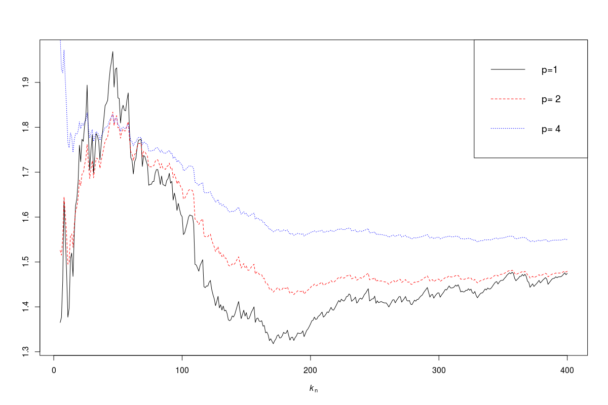
Figure 1: Hill type plots of the estimator $\hat{\gamma}(n)^{-1}$ for the Danish fire insurance claim with different $p$ values.

6 Proofs

6.1 Strong consistency

Proof of Lemma 2.2..

Let $F_{n}$ denote the empirical distribution function of the sample $U_{1}$, $\ldots$, $U_{n}$. Then, integrating by parts, we have

$$\begin{split}&\frac{1}{k}\sum_{i=1}^{k}\left(-\log\frac{U_{i,n}}{U_{k+1,n}}\right)^{p}=\frac{n}{k}\int_{(0,U_{k,n}]}\left(-\log\frac{u}{U_{k+1,n}}\right)^{p}\mathrm{d}F_{n}(u)\\ &=\frac{n}{k}\left[F_{n}(U_{k,n})\!\left(\!-\log\frac{U_{k,n}}{U_{k+1,n}}\right)^{p}\!+\!\int_{0}^{U_{k,n}}\!\!F_{n}(u)\frac{p}{u}\left(-\log\frac{u}{U_{k+1,n}}\right)^{p-1}\!\mathrm{d}u\right]\\ &=\left(-\log\frac{U_{k,n}}{U_{k+1,n}}\right)^{p}+p\frac{n}{k}\int_{0}^{U_{k,n}/U_{k+1,n}}F_{n}(U_{k+1,n}s)(-\log s)^{p-1}\frac{1}{s}\mathrm{d}s.\end{split}$$ (20)

Theorem 1 by Wellner [19] implies that

$$\frac{n}{k}U_{k,n}\to 1\quad\text{a.s.~{}whenever }\,k_{n}/\log\log n\to\infty.$$ (21)

Thus, the first term in the right-hand side of (20) tends to 0 a.s. For the second term

$$\begin{split}&\frac{n}{k}\int_{0}^{U_{k,n}/U_{k+1,n}}F_{n}(U_{k+1,n}s)(-\log s)^{p-1}s^{-1}\mathrm{d}s\\ &=\frac{n}{k}U_{k+1,n}\int_{0}^{U_{k,n}/U_{k+1,n}}(-\log s)^{p-1}\mathrm{d}s\\ &\quad+\frac{n}{k}\int_{0}^{U_{k,n}/U_{k+1,n}}(F_{n}(U_{k+1,n}s)-U_{k+1,n}s)(-\log s)^{p-1}s^{-1}\mathrm{d}s\\ &=:I_{n}+II_{n}.\end{split}$$

Again by (21)

$$I_{n}\to\int_{0}^{1}(-\log s)^{p-1}\mathrm{d}s=\Gamma(p)\quad\text{a.s.}$$ (22)

For the second term, choosing $\nu\in(0,1/2)$, we have

$$\begin{split}II_{n}&\sim\int_{0}^{1}\frac{F_{n}(U_{k+1,n}s)-U_{k+1,n}s}{U_{k+1,n}s}(-\log s)^{p-1}\mathrm{d}s\\ &=\int_{0}^{1}\frac{F_{n}(U_{k+1,n}s)-U_{k+1,n}s}{(U_{k+1,n}s)^{1/2-\nu}}(-\log s)^{p-1}(U_{k+1,n}s)^{-1/2-\nu}\mathrm{d}s\\ &\leq\sup_{u\leq U_{k+1,n}}\frac{|F_{n}(u)-u|}{u^{1/2-\nu}}U_{k+1,n}^{-1/2-\nu}\int_{0}^{1}(-\log s)^{p-1}s^{-1/2-\nu}\mathrm{d}s\\ &\leq C\left(\frac{\log\log n}{k}\right)^{1/2}\,\left[\left(\frac{n}{k}\right)^{\nu}\left(\frac{n}{\log\log n}\right)^{1/2}\sup_{u\leq 2k/n}\frac{|F_{n}(u)-u|}{u^{1/2-\nu}}\right],\end{split}$$ (23)

where $C>0$ is a finite constant, not depending on $n,k_{n}$. Using Theorem 1(ii) by Einmahl and Mason [11] we see that the last term in (23) is a.s. bounded, if $k_{n}\geq(\log n)^{(1-2\nu)/(2\nu)}$, which holds if $\nu$ is close enough to $1/2$. The first term in (23) tends to 0. From (22), (23), and (20) the statement follows. ∎

Proof of Theorem 2.3..

By the Potter bounds ([3, Theorem 1.5.6]), for any $A>1$, $\varepsilon>0$ there exist $x_{0}=x_{0}(A,\varepsilon)$ such that

$$A^{-1}(y/x)^{-\varepsilon}\leq\frac{\ell(x)}{\ell(y)}\leq A(y/x)^{\varepsilon}\quad\text{for any }\,0<x\leq y\leq x_{0}.$$ (24)

Since $k/n\to 0$, equation (21) implies $U_{k+1,n}\to 0$ a.s. Therefore, for $n$ large enough a.s.

$$\begin{split}S_{n}(p)&=\frac{1}{k}\sum_{i=1}^{k}\left(\log\frac{U_{i,n}^{-\gamma}\ell(U_{i,n})}{U_{k+1,n}^{-\gamma}\ell(U_{k+1,n})}\right)^{p}\\ &\leq\frac{1}{k}\sum_{i=1}^{k}\left(-(\gamma+\varepsilon)\log\frac{U_{i,n}}{U_{k+1,n}}+\log A\right)^{p}.\end{split}$$ (25)

First let $p\leq 1$. Using the subadditivity $(a+b)^{p}\leq a^{p}+b^{p}$, $a,b>0$, by Lemma 2.2 we obtain a.s.

$$\begin{split}\limsup_{n\to\infty}S_{n}(p)&\leq(\gamma+\varepsilon)^{p}\limsup_{n\to\infty}\frac{1}{k}\sum_{i=1}^{k}\left(-\log\frac{U_{i,n}}{U_{k+1,n}}\right)^{p}+(\log A)^{p}\\ &=(\gamma+\varepsilon)^{p}\Gamma(p+1)+(\log A)^{p}.\end{split}$$

Letting $A\downarrow 1$ and $\varepsilon\downarrow 0$ we have a.s.

$$\limsup_{n\to\infty}S_{n}(p)\leq\gamma^{p}\Gamma(p+1).$$

Next, let $p>1$. The convexity of the function $x^{p}$ implies that for any $\varepsilon^{\prime}>0$, for $a,b>0$

$$\begin{split}(a+b)^{p}&\leq(1+\varepsilon^{\prime})a^{p}+\left(1-(1+\varepsilon^{\prime})^{-1/(p-1)}\right)^{-(p-1)}b^{p}\\ &=:(1+\varepsilon^{\prime})a^{p}+C_{\varepsilon^{\prime}}b^{p}.\end{split}$$ (26)

Therefore, using Lemma 2.2 and (25), we obtain a.s.

$$\begin{split}&\limsup_{n\to\infty}S_{n}(p)\\ &\leq(\gamma+\varepsilon)^{p}(1+\varepsilon^{\prime})\limsup_{n\to\infty}\frac{1}{k}\sum_{i=1}^{k}\left(-\log\frac{U_{i,n}}{U_{k+1,n}}\right)^{p}+C_{\varepsilon^{\prime}}(\log A)^{p}\\ &=(\gamma+\varepsilon)^{p}(1+\varepsilon^{\prime})\Gamma(p+1)+C_{\varepsilon^{\prime}}(\log A)^{p}.\end{split}$$

As $A\downarrow 1$, $\varepsilon\downarrow 0$, $\varepsilon^{\prime}\downarrow 0$, we have a.s.

$$\limsup_{n\to\infty}S_{n}(p)\leq\gamma^{p}\Gamma(p+1).$$

For the lower bound choose $\varepsilon\in(0,\gamma)$. As in (25), by (24) for $n$ large enough a.s.

$$S_{n}(p)\geq\frac{1}{k}\sum_{i=1}^{k}\left(-(\gamma-\varepsilon)\log\frac{U_{i,n}}{U_{k+1,n}}-\log A\right)_{+}^{p},$$

where $a_{+}=\max\{a,0\}$ stands for the positive part. For $p\leq 1$ the subadditivity implies that $(a-b)_{+}^{p}\geq a^{p}-b^{p}$ for $a,b>0$, while for $p>1$ similarly as in (26)

$$(a-b)_{+}^{p}\geq\frac{1}{1+\varepsilon^{\prime}}a^{p}-\frac{C_{\varepsilon}}{1+\varepsilon^{\prime}}b^{p}.$$

Using these inequalities, we obtain as above that a.s.

$$\liminf_{n\to\infty}S_{n}(p)\geq\gamma^{p}\Gamma(p+1),$$

which completes the proof. ∎

6.2 Asymptotic normality

First we need two simple auxiliary lemmas.

Lemma 6.1.

For $a\in(0,1/2)$, $b\in(-1/2,1/2)$, and $a+b>0$ we have

$$|(a+b)^{p}-a^{p}|\leq\begin{cases}p|b|,&p\geq 1,\\ 2|b|a^{p-1},&p\leq 1.\end{cases}$$

Proof.

Simply $(a+b)^{p}-a^{p}=bp\xi^{p-1}$, with $\xi$ being between $a$ and $a+b$. If $b>-a/2$ then $\xi\in[a/2,1]$, thus

$$\left|(a+b)^{p}-a^{p}\right|\leq|b|p\left((a/2)^{p-1}\vee 1\right).$$

If $b<-a/2$ then $\xi\leq a$, thus $\xi^{p-1}\leq a^{p-1}$ for $p\geq 1$, and

$$\left|(a+b)^{p}-a^{p}\right|\leq|b|pa^{p-1}.$$

While if $b<-a/2$ and $p<1$

$$\begin{split}|(a+b)^{p}-a^{p}|&=(a-|b|+|b|)^{p}-(a-|b|)^{p}\leq|b|^{p}\\ &=|b||b|^{p-1}\leq|b|(a/2)^{p-1}.\end{split}$$

∎

Lemma 6.2.

For $x\geq p>0$ we have

$$\int_{x}^{\infty}e^{-y}y^{p}\mathrm{d}y\leq x^{p+1}e^{-x}(x-p)^{-1}.$$

Proof.

Simple calculation gives that

$$\begin{split}\int_{x}^{\infty}e^{-y}y^{p}\mathrm{d}y&=x^{p+1}e^{-x}\int_{1}^{\infty}e^{-x(u-1)+p\log u}\mathrm{d}u\\ &=x^{p+1}e^{-x}\int_{1}^{\infty}e^{-(x-p)(u-1)-p(u-1-\log u)}\mathrm{d}u\\ &\leq x^{p+1}e^{-x}\int_{1}^{\infty}e^{-(x-p)(u-1)}\mathrm{d}u\\ &=x^{p+1}e^{-x}(x-p)^{-1}.\end{split}$$

∎

Proof of Proposition 3.2..

To ease notation put

$$\eta(u,v)=\left(-\gamma\log u+\log\frac{\ell(uv)}{\ell(v)}\right)^{p}-\left(-\gamma\log u\right)^{p}.$$ (27)

We have by (1)

$$\begin{split}m_{p}(v)-m_{p}&=\mathbb{E}\left[\left(\log\frac{Q(1-Uv)}{Q(1-v)}\right)^{p}-\left(-\gamma\log U\right)^{p}\right]\\ &=\mathbb{E}\left[\left(-\gamma\log U+\log\frac{\ell(Uv)}{\ell(v)}\right)^{p}-\left(-\gamma\log U\right)^{p}\right]\\ &=\int_{0}^{1}\eta(u,v)\mathrm{d}u=:I_{1}(\delta)+I_{2}(\delta),\end{split}$$

where $I_{1}$, $I_{2}$ are the integrals on $(0,1-\delta)$, $(1-\delta,1)$, with $\delta\in(0,1/2)$.

First we deal with the integral on $(0,1-\delta)$. By (24), for any $\varepsilon>0$, $A>1$, there is $v_{0}>0$ such that for $v\leq v_{0}$, $u\in(0,1)$

$$A^{-1}u^{\varepsilon}\leq\frac{\ell(uv)}{\ell(v)}\leq Au^{-\varepsilon},$$ (28)

implying that uniformly on $u\in(0,1-\delta]$

$$\frac{\log\frac{\ell(uv)}{\ell(v)}}{-\log u}\to 0\quad\text{as }v\downarrow 0.$$ (29)

Writing

$$\frac{\ell(uv)-\ell(v)}{\ell(v)}=\frac{a(v)}{\ell(v)}\frac{\ell(uv)-\ell(v)}{a(v)},$$

we see that the first factor tends to 0 by (7) and the second factor is bounded by (6). Therefore, uniformly in $u\in[0,1]$

$$\log\frac{\ell(uv)}{\ell(v)}\sim\frac{a(v)}{\ell(v)}\frac{\ell(uv)-\ell(v)}{a(v)}\quad\text{as }v\downarrow 0.$$ (30)

By (29) and (30), if (8) holds then, uniformly on $u\in[0,1-\delta]$,

$$\left(1+\frac{\log\frac{\ell(uv)}{\ell(v)}}{-\gamma\log u}\right)^{p}-1\sim p(-\gamma\log u)^{-1}\,\frac{a(v)}{\ell(v)}\frac{\ell(uv)-\ell(v)}{a(v)}.$$ (31)

Thus,

$$\begin{split}I_{1}(\delta)\leq p\frac{a(v)}{\ell(v)}\,\frac{3}{2}K_{1}\gamma^{p-1}\int_{0}^{1-\delta}\left(-\log u\right)^{p-1}\mathrm{d}u.\end{split}$$ (32)

Next, we turn to $I_{2}$. Note that (30) holds, but (29) does not, because $\log u$ can be small. Choosing $\delta>0$ small enough we can achieve that $-\gamma\log(1-\delta)\in(0,1/2)$ and by (30) also that $\log\ell(uv)/\ell(v)\in(-1/2,1/2)$ for $v$ small and $u\in[1-\delta,1]$. Therefore, we can apply Lemma 6.1 with $a=-\gamma\log u$ and $b=\log(\ell(uv)/\ell(v))$ together with (30) and (6), and we obtain for $p\leq 1$

$$\begin{split}\left|\eta(u,v)\right|&\leq 2\left|\log\frac{\ell(uv)}{\ell(v)}\right|\,(-\gamma\log u)^{p-1}\\ &\leq\frac{a(v)}{\ell(v)}2K_{1}(-\gamma\log u)^{p-1}.\end{split}$$

While, for $p\geq 1$

$$\begin{split}\left|\eta(u,v)\right|\leq p\left|\log\frac{\ell(uv)}{\ell(v)}\right|\leq p\frac{a(v)}{\ell(v)}K_{1}.\end{split}$$

Summarizing,

$$I_{2}(\delta)\leq\begin{cases}\frac{a(v)}{\ell(v)}2K_{1}\gamma^{p-1}\int_{1-\delta}^{1}(-\log u)^{p-1}\mathrm{d}u,&p\leq 1,\\ p\frac{a(v)}{\ell(v)}K_{1}\delta,&p\geq 1.\end{cases}$$ (33)

The bounds (32) and (33) imply the statement. ∎

Proof of Proposition 3.3..

The difference compared to the previous proof is that (6) does not hold uniformly in $[0,1]$, which implies that the integral on $[0,\delta]$ has to be treated differently.

By Theorem 3.1.4 in [3] (translating the results from infinity to zero, by defining $\overline{\ell}(x)=\ell(x^{-1})$, $\overline{a}(x)=a(x^{-1})$)

$$\limsup_{v\downarrow 0}\sup_{u\in[\delta,1]}\frac{|\ell(uv)-\ell(v)|}{a(v)}=:K_{1}(\delta)<\infty.$$

This implies that the bound (33) on $[1-\delta,1]$ remains true and on $[\delta,1-\delta]$ as in (32) we have

$$\int_{\delta}^{1-\delta}\eta(u,v)\mathrm{d}u\leq p\frac{a(v)}{\ell(v)}\,\frac{3}{2}K_{1}\gamma^{p-1}\int_{\delta}^{1-\delta}\left(-\log u\right)^{p-1}\mathrm{d}u.$$ (34)

Recall (27) and let

$$J_{1}=\int_{0}^{b(v)}\eta(u,v)\mathrm{d}u,\quad J_{2}=\int_{b(v)}^{\delta}\eta(u,v)\mathrm{d}u,$$ (35)

where

$$b(v)=\left(\frac{a(v)}{\ell(v)}\right)^{2}\wedge e^{-2p}.$$ (36)

By Theorem 3.1.4 in [3] for any $\varepsilon>0$ there is $v_{0}(\varepsilon)>0$ and $K_{2}(\varepsilon)>0$ such that

$$\frac{|\ell(uv)-\ell(v)|}{a(v)}\leq K_{2}(\varepsilon)u^{-\varepsilon}\quad\text{for all }u\leq 1,v\leq v_{0}(\varepsilon).$$ (37)

By (36) and (11) for $\varepsilon_{1}>0$ small enough

$$p\frac{a(v)}{\ell(v)}b(v)^{-\varepsilon_{1}}\to 0.$$ (38)

Using (37), for $u\geq b(v)$

$$\frac{|\ell(uv)-\ell(v)|}{\ell(v)}\leq K_{2}(\varepsilon_{1})\frac{a(v)}{\ell(v)}u^{-\varepsilon_{1}}\leq K_{2}(\varepsilon_{1})\frac{a(v)}{\ell(v)}b(v)^{-\varepsilon_{1}}\to 0,$$

therefore

$$\left|\log\frac{\ell(uv)}{\ell(v)}\right|\sim\frac{|\ell(uv)-\ell(v)|}{\ell(v)}\leq K_{2}(\varepsilon_{1})\frac{a(v)}{\ell(v)}u^{-\varepsilon_{1}}.$$

By (38) for $u\in[b(v),\delta]$ the asymptotic equality in (31) holds, thus for $J_{2}$ in (35)

$$\begin{split}J_{2}&\sim\int_{b(v)}^{\delta}(-\gamma\log u)^{p}p(-\gamma\log u)^{-1}\frac{a(v)}{\ell(v)}\frac{\ell(uv)-\ell(v)}{a(v)}\mathrm{d}u\\ &\leq p\frac{a(v)}{\ell(v)}K_{2}(\varepsilon_{1})\int_{b(v)}^{\delta}(-\gamma\log u)^{p-1}u^{-\varepsilon_{1}}\,\mathrm{d}u\\ &\leq p\frac{a(v)}{\ell(v)}K_{2}(\varepsilon_{1})(1-\varepsilon_{1})^{-p}\gamma^{p-1}\Gamma(p),\end{split}$$ (39)

where at the last inequality we used that

$$\begin{split}\int_{0}^{1}(-\log u)^{p-1}u^{-\varepsilon_{1}}\,\mathrm{d}u&=\int_{0}^{\infty}y^{p-1}e^{-(1-\varepsilon_{1})y}\mathrm{d}y\\ &=(1-\varepsilon_{1})^{-p}\,\Gamma(p).\end{split}$$

On $(0,b(v))$ using (28), $b(v)\to 0$, Lemma 6.2, and that $-\log b(v)-p\geq(-\log b(v))/2$ we obtain for $v$ small enough

$$\begin{split}J_{1}&\leq 2\int_{0}^{b(v)}(-(\gamma+\varepsilon)\log u+\log A)^{p}\,\mathrm{d}u\\ &\leq 2(\gamma+2\varepsilon)^{p}\int_{0}^{b(v)}(-\log u)^{p}\,\mathrm{d}u\\ &=2(\gamma+2\varepsilon)^{p}\int_{-\log b(v)}^{\infty}y^{p}e^{-y}\mathrm{d}y\\ &\leq 2(\gamma+2\varepsilon)^{p}(-\log b(v))^{p+1}e^{\log b(v)}(-\log b(v)-p)^{-1}\\ &\leq 4(\gamma+2\varepsilon)^{p}\,(-\log b(v))^{p}\,b(v).\end{split}$$ (40)

Note that for $\log x>p$

$$\begin{split}\frac{(\log x)^{p}}{x}\frac{e^{p}}{p^{p}}&=\exp\left\{-p\left(\frac{\log x}{p}-1-\log\frac{\log x}{p}\right)\right\}\\ &=\exp\left\{-ph\left(\frac{\log x}{p}\right)\right\}.\end{split}$$

Thus with $x=b(v)^{-1}$

$$\begin{split}\left(\frac{e}{p}\right)^{p}(-\log b(v))^{p}\,b(v)&=\exp\left\{-ph\left(2\vee\frac{-2\log(a(v)/\ell(v))}{p}\right)\right\}\\ &=\left(\frac{a(v)}{\ell(v)}\right)^{\frac{p}{-\log(a(v)/\ell(v))}h\left(2\vee\frac{-2\log(a(v)/\ell(v))}{p}\right)}.\end{split}$$

Now the result follows from the monotonicity of $h$ and by the Stirling formula. Indeed, continuing (40) for any $\varepsilon_{2}>0$ for $v$ small enough

$$J_{1}\leq\frac{4}{\sqrt{{p\pi}}}(\gamma+2\varepsilon)^{p}\,\Gamma(p+1)\left(\frac{a(v)}{\ell(v)}\right)^{\nu_{\beta}-\varepsilon_{2}}.$$

Combining with (39), (34), and (33) the result follows. ∎

6.3 Asymptotics for large $p$

Proof of Proposition 4.2..

We follow the proof of Theorem 2.1 in [4]. Fix $\varepsilon>0$, and let $r\in[1,2]$. Using the Markov inequality, the Marcinkiewicz–Zygmund inequality (see e.g. [15, 2.6.18]), and the subadditivity we have

$$\begin{split}&\mathbb{P}\left(\frac{|Z_{n}(p,v)-nm_{p}(v)|}{nm_{p}(v)}>\varepsilon\right)\\ &\leq(\varepsilon nm_{p}(v))^{-r}\mathbb{E}|Z_{n}(p,v)-nm_{p}(v)|^{r}\\ &\leq c_{r}(\varepsilon nm_{p}(v))^{-r}\mathbb{E}\left(\sum_{i=1}^{n}(Y_{i}(v)^{p}-m_{p}(v))^{2}\right)^{r/2}\\ &\leq c_{r}(\varepsilon nm_{p}(v))^{-r}n\mathbb{E}|Y(v)^{p}-m_{p}(v)|^{r}\\ &\leq c_{r}\varepsilon^{-r}n^{1-r}\frac{m_{rp}(v)}{m_{p}(v)^{r}}.\end{split}$$ (41)

By Lemma 4.1 for any $\varepsilon_{1}>0$ we can choose $v_{0}>0$ and $p_{0}>0$ such that for $v\in(0,v_{0})$ and $p>p_{0}$

$$\frac{m_{rp}(v)}{m_{p}(v)^{r}}\leq\frac{(\gamma+\varepsilon_{1})^{rp}\Gamma(rp+1)}{(\gamma-\varepsilon_{1})^{rp}\Gamma(p+1)^{r}}\leq(1+\varepsilon_{2})^{p}\frac{\Gamma(rp+1)}{\Gamma(p+1)^{r}},$$

with $\varepsilon_{2}=2\varepsilon_{2}/(\gamma-\varepsilon_{1})$. Thus, by the Stirling formula

$$\begin{split}&\limsup_{p\to\infty}p^{-1}\log\frac{m_{rp}(v)}{n^{r-1}m_{p}(v)^{r}}\\ &\leq\log(1+\varepsilon_{2})+r\log r-(r-1)\liminf_{p\to\infty}\frac{\log n}{p}\\ &\leq\log(1+\varepsilon_{2})+r\log r-(r-1)\alpha.\end{split}$$ (42)

As $\alpha>1$ we can choose $r\in[1,2]$ such that $r\log r-(r-1)\alpha<0$. Then choosing $\varepsilon_{1}$ small enough we see that the right-hand side in (42) is negative, implying that the right-hand side in (41) tends to 0. ∎

Proof of Proposition 4.3..

By Lyapunov’s theorem (see e.g. Theorem 27.3 in Billingsley [2]) it is enough to show that for some $\delta>0$ uniformly in $v$

$$\frac{n}{(\sqrt{n}\sigma_{p}(v))^{2+\delta}}\mathbb{E}|Y(v)^{p}-m_{p}(v)|^{2+\delta}\to 0$$

as $n\to\infty$. By Lemma 4.1 $\sigma_{p}(v)\sim\sqrt{m_{2p}(v)}$ as $p\to\infty$. Thus we have to show that

$$\frac{m_{p(2+\delta)}(v)}{n^{\delta/2}m_{2p}(v)^{1+\delta/2}}\to 0.$$

As in the proof of Proposition 4.2

$$\begin{split}&\limsup_{p\to\infty}p^{-1}\log\frac{m_{p(2+\delta)}(v)}{n^{\delta/2}m_{2p}(v)^{1+\delta/2}}\\ &\leq-\frac{\delta}{2}\alpha+\log(1+\varepsilon)+(2+\delta)\log(1+\delta/2).\end{split}$$

We have to choose $\delta>0$ such that

$$\frac{2}{\delta}(2+\delta)\log\left(1+\frac{\delta}{2}\right)<\alpha.$$

This is possible for $\alpha>2$. ∎

Acknowledgements. PK’s research was partially supported by the János Bolyai Research Scholarship of the Hungarian Academy of Sciences, by the NKFIH grant FK124141, by the Ministry of Human Capacities, Hungary grant 20391-3/2018/FEKUSTRAT and by the EU-funded Hungarian grant EFOP-3.6.1-16-2016-00008. LV’s research was partially supported by the Ministry of Human Capacities, Hungary grant TUDFO/47138-1/2019-ITM.

References

• [1] A. Agresti. Categorical data analysis. Wiley Series in Probability and Statistics. Wiley-Interscience [John Wiley & Sons], New York, second edition, 2002.
• [2] P. Billingsley. Probability and measure. Wiley Series in Probability and Mathematical Statistics. John Wiley & Sons, Inc., New York, third edition, 1995. A Wiley-Interscience Publication.
• [3] N. H. Bingham, C. M. Goldie, and J. L. Teugels. Regular variation, volume 27 of Encyclopedia of Mathematics and its Applications. Cambridge University Press, Cambridge, 1989.
• [4] L. Bogachev. Limit laws for norms of IID samples with Weibull tails. J. Theoret. Probab., 19(4):849–873, 2006.
• [5] G. Ciuperca and C. Mercadier. Semi-parametric estimation for heavy tailed distributions. Extremes, 13(1):55–87, 2010.
• [6] S. Csörgő and D. M. Mason. Central limit theorems for sums of extreme values. Math. Proc. Cambridge Philos. Soc., 98(3):547–558, 1985.
• [7] S. Csörgő and L. Viharos. On the asymptotic normality of Hill’s estimator. Math. Proc. Cambridge Philos. Soc., 118(2):375–382, 1995.
• [8] L. de Haan and A. Ferreira. Extreme value theory. Springer Series in Operations Research and Financial Engineering. Springer, New York, 2006. An introduction.
• [9] P. Deheuvels, E. Haeusler, and D. M. Mason. Almost sure convergence of the Hill estimator. Math. Proc. Cambridge Philos. Soc., 104(2):371–381, 1988.
• [10] A. L. M. Dekkers, J. H. J. Einmahl, and L. de Haan. A moment estimator for the index of an extreme-value distribution. Ann. Statist., 17(4):1833–1855, 1989.
• [11] J. H. J. Einmahl and D. M. Mason. Laws of the iterated logarithm in the tails for weighted uniform empirical processes. Ann. Probab., 16(1):126–141, 1988.
• [12] P. Embrechts, C. Klüppelberg, and T. Mikosch. Modelling extremal events, volume 33 of Applications of Mathematics (New York). Springer-Verlag, Berlin, 1997. For insurance and finance.
• [13] P. Hall. On some simple estimates of an exponent of regular variation. J. Roy. Statist. Soc. Ser. B, 44(1):37–42, 1982.
• [14] B. M. Hill. A simple general approach to inference about the tail of a distribution. Ann. Statist., 3(5):1163–1174, 1975.
• [15] V. V. Petrov. Limit theorems of probability theory, volume 4 of Oxford Studies in Probability. The Clarendon Press, Oxford University Press, New York, 1995.
• [16] S. Resnick. Discussion of the Danish data on large fire insurance losses. 27(1):139–151, 1997.
• [17] M. Schlather. Limit distributions of norms of vectors of positive i.i.d. random variables. Ann. Probab., 29(2):862–881, 2001.
• [18] J. Segers. Residual estimators. J. Statist. Plann. Inference, 98(1-2):15–27, 2001.
• [19] J. A. Wellner. Limit theorems for the ratio of the empirical distribution function to the true distribution function. Z. Wahrsch. Verw. Gebiete, 45(1):73–88, 1978.