Nonradiative $\bm{\alpha^{7}m}$ QED effects in Lamb shift of helium triplet states

Abstract

Theoretical predictions for the Lamb shift in helium are limited by unknown quantum electrodynamic effects of the order $\alpha^{7}m$, where $\alpha$ is the fine-structure constant and $m$ is the electron mass. We make an important step towards the complete calculation of these effects by deriving the most challenging part, which is induced by the virtual photon exchange between all three helium particles, the two electrons, and the nucleus. The complete calculation of the $\alpha^{7}m$ effect including the radiative corrections will allow comparing of the nuclear charge radii determined from the electronic and muonic helium atoms and thus provide a stringent test of the Standard Model of fundamental interactions.

High-precision spectroscopy of the hydrogen atom enables the determination of the Rydberg constant mohr:16:codata and provides a stringent test of the Standard Model of fundamental interactions, through a comparison of the Lamb shift of ordinary (electronic) hydrogen and the muonic hydrogen $\mu$H pohl:10 ; antognini:13 . This was made possible by the success of the theory of the hydrogen atom, notably, progress in calculations of the higher-order two-loop quantum electrodynamic (QED) effects yerokhin:18:hydr ; karshenboim:18 .

The present investigation is a part of a long and challenging project, the aim of which is to extend the high-precision spectroscopic tests of the Standard Model to two-electron systems; specifically, the helium atom and light helium-like ions. Helium is better suited for experimental studies than hydrogen because of the presence of several narrow lines in the spectrum. As a consequence, a number of recent helium experiments reached a relative precision of a few parts in $10^{-12}$ zheng:02 ; rooij:11 ; luo:13 ; notermans:14 ; luo:16 ; zheng:17 ; rengelink:18 ; kato:18 . This experimental precision is sufficient for an accurate spectroscopic determination of the nuclear charge radii of ³He and ⁴He.

Such determination is of great importance because it would allow effective comparison of spectroscopic measurements in ordinary helium and in muonic helium $\mu$He pohl:16:leap . A similar comparison in electronic and muonic hydrogen pohl:10 ; antognini:13 revealed a large discrepancy, which remained unexplained for a decade and became known as the proton-radius puzzle. Recent experiments beyer:17 ; bezginov:19 ; xiong:19 indicate that this puzzle was most likely caused by unidentified systematic effects in several previous measurements in electronic hydrogen. These findings will have a significant impact on the future development of hydrogen spectroscopy.

Our recent investigations indicate that similar problems might be present also in helium spectroscopy. Specifically, in Refs. pachucki:15:jpcrd ; patkos:16:triplet ; patkos:17:singlet we obtained accurate theoretical predictions for the isotope shifts of various transition energies in helium. Combining these predictions with the available experimental data shiner:95 ; pastor:04 ; rooij:11 ; pastor:12 , results were obtained for the difference $\delta r^{2}$ of the mean-square nuclear charge radii of ³He and ⁴He. Comparing values of $\delta r^{2}$ from different transitions, we found significant inconsistencies pachucki:15:jpcrd ; patkos:16:triplet . Since then, an independent measurement of the $2^{3}S$-$2^{3}P$ transition energy zheng:17 found a $20\,\sigma$ shift from the previous experimental result pastor:12 , which led to a better, albeit not perfect, agreement among different $\delta r^{2}$ values. This means that further work is needed for a reliable determination of $\delta r^{2}$.

A more stringent test of the helium spectroscopic results could be accomplished if one extracts the absolute nuclear radius and compares it with the corresponding value derived from the spectroscopy of the muonic helium. In order to realize this project, a significant advance in theory of the helium Lamb shift is needed; specifically, a complete calculation of the QED effects of order $\alpha^{7}\,m$. The best existing calculations of the helium energy levels pachucki:06:he ; pachucki:17:heSummary are complete through order $\alpha^{6}m$. The higher-order $\alpha^{7}m$ were calculated for simpler cases; namely, for the fine structure pachucki:06:prl:he ; pachucki:09:hefs ; pachucki:10:hefs , the hydrogen molecular ions, and the antiprotonic helium korobov:13 ; korobov:14 .

The first step on the path towards the complete calculation of the $\alpha^{7}m$ QED effects was made in our previous work yerokhin:18:betherel , in which we calculated the relativistic correction to the so-called Bethe logarithm. In the present investigation we take the next step, which is the calculation of the $\alpha^{7}m$ correction induced by an exchange of two and three virtual photons between the two electrons and between the electrons and the nucleus. The key part is the derivation of the corresponding effective operator $H^{(7)}_{\rm exch}$. This challenging problem was successfully solved in the present work, and the final result is compact and very simple. We leave for the future the third and the last step, which is the calculation of the radiative $\alpha^{7}m$ corrections. After that, the calculation of the $\alpha^{7}m$ QED effects for the triplet states of two-electron atoms will be completed, enabling the spectroscopic determinations of the nuclear charge radii of the helium atom and light helium-like ions.

I NRQED Approach

The derivation in the present work is performed within the Nonrelativistic QED (NRQED) method, originally introduced by Caswell and Lepage caswell:86 . This method is based on the NRQED Lagrangian, which we obtain by the Foldy-Wouthuysen transformation of the Dirac Hamiltonian in the presence of an electromagnetic field as described in Appendix A.

Once the NRQED Lagrangian is obtained, the Feynman path-integral approach is used to derive various corrections to the nonrelativistic multi-electron propagator $G(t-t^{\prime})$, where $t$ and $t^{\prime}$ are the common time of the out and the in electrons, correspondingly. The Fourier transform over the time variable yields the propagator in the energy-coordinate representation,

$$G(E)=\frac{1}{E-H_{0}-\Sigma(E)},$$

where $H_{0}$ is the Schrödinger-Coulomb Hamiltonian of an $N$-electron atom. $H_{0}$ may also include the nucleus as a dynamic particle, but this is not needed in the present work, so we assume the nucleus to be a static source of the Coulomb field. The operator $\Sigma(E)$ incorporates various corrections due to the photon exchange, the electron and photon self-energy, etc.

The energy of a bound state $|\phi\rangle$ is obtained as a position of the pole of the matrix element of $G(E)$ between the nonrelativistic wave functions of the reference state,

$$\langle\phi|G(E)|\phi\rangle = \frac{1}{E-E_{0}}+\frac{1}{(E-E_{0})^{2}}\,\langle\phi|\Sigma(E)|\phi\rangle$$ (1)

$$+\frac{1}{(E-E_{0})^{2}}\,\langle\phi|\Sigma(E)\,\frac{1}{E-H_{0}}\,\Sigma(E)|\phi\rangle+\ldots$$

$$= \frac{1}{E-E_{0}-\sigma(E)}\,,$$

where

$$\sigma(E)=\langle\phi|\Sigma(E)|\phi\rangle+\langle\phi|\Sigma(E)\,\frac{1}{(E-H_{0})^{\prime}}\,\Sigma(E)|\phi\rangle+\ldots\,.$$ (2)

The resulting bound-state energy $E$ (i.e. the position of the pole) is

$$E=E_{0}+\sigma(E_{0})+\sigma(E_{0})\,\frac{\partial\sigma(E_{0})}{\partial E_{0}}+\ldots\,.$$ (3)

We assume that $E$ can be expanded in a power series of the fine-structure constant $\alpha$,

$$E(\alpha)= \ m\alpha^{2}\,E^{(2)}+m\alpha^{4}\,E^{(4)}$$

$$\ +m\alpha^{5}\,E^{(5)}+m\alpha^{6}\,E^{(6)}+m\alpha^{7}\,E^{(7)}+\ldots\,,$$ (4)

where the expansion coefficients $E^{(n)}$ may contain finite powers of $\ln\alpha$. These coefficients can be expressed as expectation values of some effective Hamiltonians with the nonrelativistic wave function. The derivation of these effective Hamiltonians is the central problem of the NRQED method. While the leading-order expansion terms are simple, formulas become increasingly complicated for higher orders in $\alpha$.

The present status of the theory of helium energy levels up to the order $\alpha^{6}m$ is summarized in our recent review pachucki:17:heSummary . In the present investigation we are interested in the next-order $\alpha^{7}m$ contribution $E^{(7)}$.

II $\bm{\alpha^{7}\,m}$ effects

The contribution of order $\alpha^{7}m$ can be represented as a sum of four parts,

$$E^{(7)}=\big{<}H^{(7)}_{\rm exch}\big{>}+\big{<}H^{(7)}_{\rm rad}\big{>}+2\,\big{<}H^{(4)}\,\frac{1}{(E_{0}-H_{0})^{\prime}}\,H^{(5)}\big{>}+E_{L}\,.$$ (5)

The first two terms here are the expectation values of the effective Hamiltonians of order $\alpha^{7}m$ induced by the photon exchange and the radiative effects, respectively. The third term is the second-order perturbative correction induced by the Breit Hamiltonian $H^{(4)}$ and the effective Hamiltonian $H^{(5)}$ of order $\alpha^{5}\,m$, whereas the last term is the relativistic correction to the Bethe logarithm.

The goal of the present investigation is the derivation of the effective Hamiltonian $H^{(7)}_{\rm exch}$ , which originates exclusively from the photon-exchange diagrams. It is convenient to split it into three parts,

$$\big{<}H^{(7)}_{\rm exch}\big{>}=E_{L}^{\Lambda}+E_{M}+E_{H}\,,$$ (6)

which are induced by momenta $k$ of the exchanged virtual photons of the order $m\alpha^{2}$, $m\alpha$, and $m$, respectively. These three terms will be referred to as the low-energy, middle-energy, and high-energy parts, correspondingly. The derivation will be performed in the Coulomb gauge unless explicitly stated otherwise.

The middle-energy and the high-energy parts $E_{M}$ and $E_{H}$ contain singular operators that need a systematic regularization. In the present work we will use the dimensional regularization, with the dimension $d=3-2\epsilon$. Singular contributions of order $1/\epsilon$ will be canceled algebraically in momentum space. After that, the result will be transformed into the coordinate representation, where it can be calculated numerically.

$E_{M}$ consists of the two- and three-photon exchange contributions. The two-photon exchange part is the most complicated one. In order to eliminate possible errors, its derivation is performed by two independent methods, namely, by the NRQED approach and by the scattering amplitude method. The derivation of the three-photon part from the scattering amplitude is too complicated to be feasible, so we perform it only within the NRQED approach. There are only a few three-photon diagrams and the corresponding derivation within the NRQED approach is sufficiently tractable to be properly checked. The high-energy part $E_{H}$ is derived from the two-photon exchange scattering amplitude, in an analogous way as it was done for the fine structure in Refs. pachucki:06:prl:he ; pachucki:09:hefs ; pachucki:10:hefs .

The low-energy contribution $E_{L}^{\Lambda}$ in Eq. (6) is a complementary part to the relativistic correction to the Bethe logarithm ($E_{L}$ in Eq. (5)) calculated in Ref. yerokhin:18:betherel . The definition of $E_{L}$ involved the cut-off photon-momentum parameter $\Lambda$. The low-energy contribution $E_{L}^{\Lambda}$ converts the $\Lambda$ regularization to the dimensional regularization used in $E_{M}$ and $E_{H}$, so that all singularities can be consistently canceled.

In our derivation we will need the $d$-dimensional generalization of the Breit Hamiltonian. For a two-electron atom, it can be written as

$$H^{(4)} \ =H^{\prime(4)}+H^{\prime\prime(4)}\,,$$ (7)

$$H^{\prime(4)} \ =-\frac{\pi\,\alpha}{m^{2}}\,\delta^{d}(r)+\sum_{a=1,2}\biggl{\{}-\frac{p_{a}^{4}}{8\,m^{3}}+\frac{\pi\,Z\alpha}{2\,m^{2}}\,\delta^{d}(r_{a})$$

$$\ -\frac{1}{4\,m^{2}}\,\sigma_{a}^{ij}\,\nabla^{i}\left[\frac{Z\,\alpha}{r_{a}}\right]_{\epsilon}p_{a}^{j}+\frac{1}{4\,m^{2}}\sigma_{a}^{ij}\,\nabla_{a}^{i}\left[\frac{\alpha}{r}\right]_{\epsilon}p_{a}^{j}\biggr{\}}\,,$$

$$H^{\prime\prime(4)} \ =-\frac{\alpha}{2\,m^{2}}\,p_{1}^{i}\,\biggl{[}\frac{\delta^{ij}}{r}+\frac{r^{i}\,r^{j}}{r^{3}}\biggr{]}_{\epsilon}\,p_{2}^{j}-\frac{\pi\,\alpha}{d\,m^{2}}\,\sigma_{1}^{ij}\,\sigma_{2}^{ij}\,\delta^{d}(r)$$

$$\ +\frac{1}{4\,m^{2}}\,\sigma_{1}^{ik}\,\sigma_{2}^{jk}\,\left(\nabla^{i}\,\nabla^{j}-\frac{\delta^{ij}}{d}\,\nabla^{2}\right)\,\left[\frac{\alpha}{r}\right]_{\epsilon}$$

$$\ -\frac{1}{2\,m^{2}}\,\biggl{(}\sigma_{1}^{ij}\,\nabla^{i}\left[\frac{\alpha}{r}\right]_{\epsilon}\,p^{j}_{2}-\sigma_{2}^{ij}\,\nabla^{i}\left[\frac{\alpha}{r}\right]_{\epsilon}\,p^{j}_{1}\biggr{)}\,,$$ (8)

where $\vec{r}=\vec{r}_{1}-\vec{r}_{2}$, $\sigma^{ij}$ is defined in Appendix B, $\delta^{d}(r)$ is the Dirac $\delta$-function in $d$ dimensions, and $\big{[}\ldots\big{]}_{\epsilon}$ denotes the $d$-dimensional generalization of the operator $\big{[}\ldots\big{]}$ written in $d=3$. The separation of $H^{(4)}$ into two parts is based on the fact that $H^{\prime(4)}$ comes from the exchange of a Coulomb photon, whereas $H^{\prime\prime(4)}$ originates from the exchange of a transverse photon.

The second-order contribution in Eq. (5) involves the Breit Hamiltonian $H^{(4)}$ and the effective $\alpha^{5}\,m$ operator $H^{(5)}$, which is the sum of the photon-exchange and radiative parts,

$$H^{(5)}=H^{(5)}_{\rm exch}+H^{(5)}_{\rm rad}\,.$$ (9)

This contribution is relatively simple. The derivation of $H^{(5)}_{\rm exch}$ is presented in Appendix D following the method described in Ref. simple , and the result in $d=3$ for triplet states is

$$H^{(5)}_{\rm exch}= \,-\frac{7}{6\,\pi}\,\frac{\alpha^{2}}{m^{2}}\,\frac{1}{r^{3}}$$ (10)

The radiative $H^{(5)}_{\rm rad}$ part is left for future investigation, alongside $H^{(7)}_{\rm rad}$.

III Low-energy part

The low-energy part comes from the virtual photon momenta of the order $k\propto m\alpha^{2}$. In order to derive formulas for the low-energy part, we start with the one-loop nonrelativistic dipole exchange contribution of the order $\alpha^{5}m$, which is

$$E_{L0} = \frac{e^{2}}{m^{2}}\int_{0}^{\infty}\frac{d^{d}k}{(2\pi)^{d}2k}\,\delta_{\perp}^{ij}(k)$$ (11)

$$\times\,\bigg{\langle}\phi\bigg{|}p_{1}^{i}\,\frac{1}{E_{0}-H_{0}-k}\,p_{2}^{j}\bigg{|}\phi\bigg{\rangle}+(1\leftrightarrow 2)\,,$$

where $\delta_{\perp}^{ij}(k)=\delta^{ij}-k^{i}k^{j}/k^{2}$. We are interested in relativistic corrections to $E_{L0}$ of order $\alpha^{7}m$. Such corrections arise through: (i) perturbations of the reference-state wave function $\phi$, the zeroth-order energy $E_{0}$ and the zeroth-order Hamiltonian $H_{0}$ by the Breit Hamiltonian $H^{(4)}$, (ii) the perturbation of the current $\vec{p}\to\delta\vec{j}$, and (iii) the retardation (quadrupole) correction. The corresponding corrections will be denoted as $E_{L1}$, $E_{L2}$, and $E_{L3}$, respectively, so

$$E_{L}^{\Lambda}=E_{L1}^{\Lambda}+E_{L2}^{\Lambda}+E_{L3}^{\Lambda}.$$ (12)

It is convenient to separate the $k$ integral in Eq. (11) into two regions,

$$\int_{0}^{\infty}dk=\int_{0}^{\Lambda}dk+\int_{\Lambda}^{\infty}dk\,,$$ (13)

where $\Lambda\equiv m\alpha^{2}\lambda$ and $\lambda$ is the dimensionless cutoff parameter. In the small-$k$ region, $k<\Lambda$, the binding effects should be accounted for to all orders. Such contributions give rise to relativistic corrections to the Bethe logarithm, already computed in Ref. yerokhin:18:betherel . In the present investigation we will be concerned with the large-$k$ region, $k>\Lambda$. In this region, $k$ is much larger than the characteristic energy of the intermediate electron states and we can use the large-$k$ expansion of the resolvent $1/(E_{0}-H_{0}-k)$.

The perturbation of Eq. (11) by the Breit Hamiltonian can be written as

$$E_{L1}^{\Lambda} = \frac{e^{2}}{m^{2}}\int_{\Lambda}^{\infty}\frac{d^{d}k}{(2\pi)^{d}2k}\,\delta_{\perp}^{ij}(k)$$ (14)

$$\times\,\delta\bigg{\langle}\phi\bigg{|}p_{1}^{i}\frac{1}{E_{0}-H_{0}-k}p_{2}^{j}\bigg{|}\phi\bigg{\rangle}+(1\leftrightarrow 2)\,,$$

where the symbol $\delta\langle\cdots\rangle$ stands for the first-order perturbation of the matrix element $\langle\cdots\rangle$ by the Breit-Hamiltonian $H^{(4)}$, which implies perturbations of the reference-state wave function $\phi$, the energy $E_{0}$ and the zeroth-order Hamiltonian $H_{0}$. Since $k$ is much bigger than $H_{0}-E_{0}$, we can expand the integrand of Eq. (14) in large $k$, keeping only the $1/k^{2}$ term, while $1/k$ contributes at the lower order of $\alpha^{6}\,m$. The result is

$$\delta\bigg{\langle}\phi\bigg{|}p_{1}^{i}\frac{1}{E_{0}-H_{0}-k}p_{2}^{j}\bigg{|}\phi\bigg{\rangle}+(1\leftrightarrow 2) = \frac{1}{k^{2}}\,\delta\big{\langle}\phi\big{|}\big{[}p_{1}^{i},\big{[}H_{0}-E_{0},p_{2}^{j}\big{]}\big{]}\big{|}\phi\rangle$$ (15)

$$= \frac{2}{k^{2}}\,\bigg{\langle}\phi\bigg{|}[p_{1}^{i},[V,p_{2}^{j}]]\frac{1}{(E_{0}-H_{0})^{\prime}}H^{(4)}\bigg{|}\phi\bigg{\rangle}+\frac{1}{k^{2}}\,\big{\langle}\phi|[p_{1}^{i},[H^{(4)},p_{2}^{j}]]\big{|}\phi\big{\rangle}\,,$$

where $V$ is the Coulomb potential. The first term is the second-order perturbation correction included in the third term of Eq. (5), so we omit it here. We thus have

$$E_{L1}^{\Lambda}=\frac{e^{2}}{m^{2}}\frac{d-1}{d}\int_{\Lambda}^{\infty}\frac{d^{d}k}{(2\pi)^{d}\,2\,k^{3}}\big{\langle}\phi\big{|}\,[p_{1}^{i},[\delta H^{(4)},p_{2}^{i}]]\,\big{|}\phi\big{\rangle}\,,$$ (16)

where $\delta H^{(4)}$ is the spin-independent part of the Breit Hamiltonian that survives the double commutator, given by (in momentum representation and in $d$ dimensions)

$$\delta H^{(4)}=-\frac{\alpha\,\pi}{d\,m^{2}}\sigma_{1}\cdot\sigma_{2}-\frac{\alpha}{m^{2}}\bigg{[}\pi+p_{1}^{i}\,\frac{4\pi}{q^{2}}\bigg{(}\delta^{ij}-\frac{q^{i}q^{j}}{q^{2}}\bigg{)}\,p^{\prime j}_{2}\bigg{]}\,.$$ (17)

Here, $\vec{q}=\vec{p}_{1}{}^{\prime}-\vec{p}_{1}$ is the momentum exchanged between electrons. All integrations are performed in the momentum space using formulas presented in Appendix C. After expanding in $\epsilon=(3-d)/2$ and then in $\alpha$, we obtain the result for the effective operator $H_{L1}$, defined as $E_{L1}^{\Lambda}=\langle H_{L1}\rangle$,

$$H_{L1} = \frac{\alpha^{2}}{m^{4}}\bigg{\{}\sigma_{1}\cdot\sigma_{2}\bigg{(}-\frac{7}{27}-\frac{1}{9}\ln{\Lambda_{\epsilon}}\bigg{)}\,q^{2}+\bigg{(}-\frac{5}{9}-\frac{1}{3}\ln{\Lambda_{\epsilon}}\bigg{)}\,\bigg{[}q^{2}+4\vec{P}_{1}\cdot\vec{P}_{2}-4\frac{\big{(}\vec{P}_{1}\cdot\vec{q}\big{)}\big{(}\vec{P}_{2}\cdot\vec{q}\big{)}}{q^{2}}\bigg{]}\bigg{\}}\,,$$ (18)

where

$$\ln{\Lambda_{\epsilon}} = \frac{1}{\epsilon}+2\ln[\alpha^{-2}]-2\ln(2\lambda)\,$$ (19)

and

$$\vec{P}_{1}=\frac{1}{2}(\vec{p}_{1}+\vec{p}_{1}{}^{\prime}),\,\,\vec{P}_{2}=\frac{1}{2}(\vec{p}_{2}+\vec{p}_{2}{}^{\prime})$$ (20)

are sums of the in and out momenta of the corresponding electron.

The second term in Eq. (12) comes from the correction to current. Specifically, $\vec{p}_{1}$ gets a correction $\delta\vec{j}_{1}$, which is

$$\delta j^{i}_{1}=i\big{[}H^{(4)},r_{1}^{i}\big{]}=-\frac{1}{2m^{3}}p_{1}^{i}p_{1}^{2}-\frac{1}{m^{2}}\frac{4\pi\alpha}{q^{\prime 2}}\bigg{(}\delta^{ij}-\frac{q^{\prime i}q^{\prime j}}{q^{\prime 2}}\bigg{)}\,p_{2}^{j}\,,$$ (21)

where $q^{\prime}$ is the exchanged momentum, and the same for $\vec{p}_{2}$. The correction $E_{L2}$ is then

$$E_{L2}^{\Lambda} = 2\frac{e^{2}}{m}\int_{\Lambda}^{\infty}\frac{d^{d}k}{(2\pi)^{d}2k}\,\delta_{\perp}^{ij}(k)\,\bigg{\langle}\phi\bigg{|}\delta j_{1}^{i}\frac{1}{E_{0}-H_{0}-k}p_{2}^{j}\bigg{|}\phi\bigg{\rangle}+(1\leftrightarrow 2)\,.$$ (22)

Expanding for large $k$ and performing the angular average, we arrive at

$$E_{L2}^{\Lambda}=\frac{e^{2}}{m}\frac{d-1}{d}\int_{\Lambda}^{\infty}\frac{d^{d}k}{(2\pi)^{d}2k^{3}}\big{\langle}\phi\big{|}\,[\delta j_{1}^{i},[V,p_{2}^{i}]]\,\big{|}\phi\big{\rangle}+(1\leftrightarrow 2)\,.$$ (23)

This expression contains three-photon $\sim\alpha^{3}$ and two-photon $\sim\alpha^{2}$ terms. The result for the effective operator $H_{L2}$, $E_{L2}^{\Lambda}=\langle H_{L2}\rangle$, is

$$H_{L2} = \frac{\alpha^{3}}{m^{3}}\bigg{\{}\bigg{[}p_{2}^{i},\bigg{[}-\bigg{[}\frac{Z}{r_{2}}\bigg{]}_{\epsilon},p_{2}^{j}\bigg{]}\bigg{]}\bigg{(}-\frac{20}{9}-\frac{4}{3}\ln{\Lambda_{\epsilon}}\bigg{)}\bigg{(}\delta^{ij}-\frac{q^{i}q^{j}}{q^{2}}\bigg{)}\frac{1}{q^{2}}+(1\leftrightarrow 2)\bigg{\}}$$ (24)

$$+\frac{\alpha^{2}}{m^{4}}\bigg{(}-\frac{20}{9}-\frac{4}{3}\ln{\Lambda_{\epsilon}}\bigg{)}\bigg{(}\frac{1}{2}\big{(}\vec{P}_{1}-\vec{P}_{2}\big{)}^{2}+\vec{P}_{1}\cdot\vec{P}_{2}+\frac{1}{4}q^{2}+\frac{\big{[}\big{(}\vec{P}_{1}-\vec{P}_{2}\big{)}\cdot\vec{q}\big{]}^{2}}{q^{2}}+2\frac{\big{(}\vec{P}_{1}\cdot\vec{q}\big{)}\big{(}\vec{P}_{2}\cdot\vec{q}\big{)}}{q^{2}}\bigg{)}$$

$$+\pi\frac{\alpha^{3}}{m^{3}}\bigg{(}\frac{4}{9}+\frac{2}{3}\ln{\Lambda_{\epsilon}}+\frac{4}{3}\ln 2-\frac{4}{3}\ln q\bigg{)}q\,.$$

$E^{\Lambda}_{L3}$ is the correction due to the retardation. We write it as

$$E_{L3}^{\Lambda} = \frac{e^{2}}{m^{2}}\int_{\Lambda}^{\infty}\frac{d^{d}k}{(2\pi)^{d}2k}\,\delta_{\perp}^{ij}(k)\,\delta_{k^{2}}\bigg{\langle}\phi\bigg{|}p_{1}^{i}\,e^{i\vec{k}\cdot\vec{r}_{1}}\frac{1}{E_{0}-H_{0}-k}p_{2}^{j}\,e^{-i\vec{k}\cdot\vec{r}_{2}}\bigg{|}\phi\bigg{\rangle}+(1\leftrightarrow 2)\,.$$ (25)

Here the symbol $\delta_{k^{2}}\big{<}\ldots\big{>}$ means that the exponent functions $e^{i\vec{k}\cdot\vec{r}_{1}}$ and $e^{-i\vec{k}\cdot\vec{r}_{2}}$ in the matrix element $\big{<}\ldots\big{>}$ are expanded in small $k$ and only the $k^{2}$ term is left. We now perform the large-$k$ expansion of the resolvent,

$$\frac{1}{E_{0}-H_{0}-k} = -\frac{1}{k}+\frac{H_{0}-E_{0}}{k^{2}}-\frac{(H_{0}-E_{0})^{2}}{k^{3}}+\frac{(H_{0}-E_{0})^{3}}{k^{4}}+\cdots\,.$$ (26)

We have to extend the expansion up to order $k^{-4}$ because of the additional $k^{2}$ from the expansion of the exponent functions. The result of the expansion is

$$E_{L3}^{\Lambda} = \frac{e^{2}}{m^{2}}\int_{\Lambda}^{\infty}\frac{d^{d}k}{(2\pi)^{d}2k^{5}}\,\delta_{\perp}^{ij}(k)\,\delta_{k^{2}}\bigg{\langle}\phi\bigg{|}p_{1}^{i}\,e^{i\vec{k}\cdot\vec{r}_{1}}(H_{0}-E_{0})^{3}\,p_{2}^{j}\,e^{-i\vec{k}\cdot\vec{r}_{2}}\bigg{|}\phi\bigg{\rangle}+(1\leftrightarrow 2)\,.$$ (27)

This expression is evaluated in Appendix E, with the result for $E_{L3}^{\Lambda}=\langle H_{L3}\rangle$,

$$H_{L3} = \frac{\alpha^{3}}{m^{3}}\bigg{\{}\bigg{[}p_{2}^{i},\bigg{[}-\bigg{[}\frac{Z}{r_{2}}\bigg{]}_{\epsilon},p_{2}^{j}\bigg{]}\bigg{]}\bigg{[}\delta^{ij}\bigg{(}\frac{184}{225}+\frac{4}{15}\ln{\Lambda_{\epsilon}}\bigg{)}+\frac{q^{i}q^{j}}{q^{2}}\bigg{(}-\frac{436}{225}-\frac{16}{15}\ln{\Lambda_{\epsilon}}\bigg{)}\bigg{]}\frac{1}{q^{2}}$$ (28)

$$+\bigg{(}-\frac{254}{225}-\frac{14}{15}\ln{\Lambda_{\epsilon}}\bigg{)}\bigg{[}p_{2}^{j},-\bigg{[}\frac{Z}{r_{2}}\bigg{]}_{\epsilon}\bigg{]}\frac{q^{j}}{q^{2}}+(1\leftrightarrow 2)\bigg{\}}+\frac{\alpha^{2}}{m^{4}}\bigg{\{}\bigg{(}\frac{124}{225}+\frac{4}{15}\ln{\Lambda_{\epsilon}}\bigg{)}\bigg{(}(\vec{P}_{1}-\vec{P}_{2})^{2}+\frac{1}{2}q^{2}\bigg{)}$$

$$+\bigg{(}\frac{136}{45}+\frac{4}{3}\ln{\Lambda_{\epsilon}}\bigg{)}\,\vec{P}_{1}\cdot\vec{P}_{2}+\bigg{(}\frac{10}{9}+\frac{2}{3}\ln{\Lambda_{\epsilon}}\bigg{)}\frac{[(\vec{P}_{1}-\vec{P}_{2})\cdot\vec{q}]^{2}}{q^{2}}+\bigg{(}\frac{112}{45}+\frac{4}{3}\ln{\Lambda_{\epsilon}}\bigg{)}\frac{(\vec{P}_{1}\cdot\vec{q})(\vec{P}_{2}\cdot\vec{q})}{q^{2}}\bigg{\}}$$

$$+\pi\frac{\alpha^{3}}{m^{3}}\bigg{(}\frac{29}{225}-\frac{1}{15}\ln{\Lambda_{\epsilon}}-\frac{2}{15}\ln 2+\frac{2}{15}\ln q\bigg{)}\,q\,.$$

The total result for the low-energy contribution is a sum of three terms in Eq. (12),

$$E_{L}^{\Lambda} = \langle H_{L}\rangle=\langle H_{L1}+H_{L2}+H_{L3}\rangle\,,$$

$$H_{L} = \frac{\alpha^{3}}{m^{3}}\bigg{\{}\bigg{[}p_{2}^{i},\bigg{[}-\bigg{[}\frac{Z}{r_{2}}\bigg{]}_{\epsilon},p_{2}^{j}\bigg{]}\bigg{]}\bigg{[}\delta^{ij}\bigg{(}-\frac{316}{225}-\frac{16}{15}\ln{\Lambda_{\epsilon}}\bigg{)}+\frac{q^{i}q^{j}}{q^{2}}\bigg{(}\frac{64}{225}+\frac{4}{15}\ln{\Lambda_{\epsilon}}\bigg{)}\bigg{]}\frac{1}{q^{2}}$$

$$+\bigg{(}-\frac{254}{225}-\frac{14}{15}\ln{\Lambda_{\epsilon}}\bigg{)}\bigg{[}p_{2}^{j},-\bigg{[}\frac{Z}{r_{2}}\bigg{]}_{\epsilon}\bigg{]}\frac{q^{j}}{q^{2}}+(1\leftrightarrow 2)\bigg{\}}+\frac{\alpha^{2}}{m^{4}}\bigg{[}\bigg{(}-\frac{14}{25}-\frac{2}{5}\ln{\Lambda_{\epsilon}}\bigg{)}(\vec{P}_{1}-\vec{P}_{2})^{2}$$

$$+\bigg{(}-\frac{188}{225}-\frac{8}{15}\ln{\Lambda_{\epsilon}}\bigg{)}q^{2}+\bigg{(}-\frac{64}{45}-\frac{4}{3}\ln{\Lambda_{\epsilon}}\bigg{)}\vec{P}_{1}\cdot\vec{P}_{2}+\frac{4}{15}\frac{(\vec{P}_{1}\cdot\vec{q})(\vec{P}_{2}\cdot\vec{q})}{q^{2}}$$

$$+\bigg{(}-\frac{10}{9}-\frac{2}{3}\ln{\Lambda_{\epsilon}}\bigg{)}\frac{[(\vec{P}_{1}-\vec{P}_{2})\cdot\vec{q}]^{2}}{q^{2}}+\sigma_{1}\cdot\sigma_{2}\bigg{(}-\frac{7}{27}-\frac{1}{9}\ln{\Lambda_{\epsilon}}\bigg{)}\,q^{2}\bigg{]}$$

$$+\pi\frac{\alpha^{3}}{m^{3}}\bigg{(}\frac{43}{75}+\frac{3}{5}\ln{\Lambda_{\epsilon}}+\frac{6}{5}\ln 2-\frac{6}{5}\ln q\bigg{)}q\,.$$

This concludes the derivation of the low-energy part $E_{L}^{\Lambda}$.

IV Middle-energy photon-exchange part $\bm{E_{M}}$

The derivation of $E_{M}$ is by far the most complicated. We start with deriving the NRQED Hamiltonian by the Foldy-Wouthuysen transformation of the Dirac Hamiltonian in the external electromagnetic field, as described in Appendix A. The result is

$$H_{\rm FW} = eA^{0}+\frac{\pi^{2}}{2m}-\frac{e}{4m}\sigma\cdot B-\frac{\pi^{4}}{8m^{3}}+\frac{e}{16m^{3}}\bigl{(}\sigma\cdot B\,\vec{\pi}^{2}+\vec{\pi}^{2}\,\sigma\cdot B\bigr{)}-\,\frac{e}{8m^{2}}\bigl{(}\vec{\nabla}\,\vec{E_{\parallel}}+\sigma^{ij}\{E_{\parallel}^{i},\pi^{j}\}\bigr{)}$$ (30)

$$+\frac{e^{2}}{8m^{3}}\vec{E}^{2}-\frac{e^{2}}{16m^{3}}B^{ij}B^{ij}-\frac{e^{2}}{4m^{2}}\sigma^{ij}A^{i}E^{j}+\frac{ie}{16m^{3}}[\sigma^{ij}\{A^{i},\pi^{j}\},\pi^{2}]-\frac{e^{2}}{8m^{3}}A^{i}\,\nabla^{j}B^{ij}\,,$$

where $\vec{E}_{\parallel}=-\vec{\nabla}V$ and $B^{ij}=\partial^{i}A^{j}-\partial^{j}A^{i}$. From this Hamiltonian we obtain the single-transverse photon vertices,

$$\delta_{\rm ST}H_{\rm FW} = -\frac{e}{m}\Bigl{(}\vec{p}\cdot\vec{A}+\frac{1}{4}\sigma\cdot B\Bigr{)}+\frac{e}{4m^{3}}\bigl{\{}\vec{p}\,{}^{2},\vec{p}\cdot\vec{A}+\frac{1}{4}\,\sigma\cdot B\bigr{\}}+\frac{e^{2}}{2m^{2}}\sigma^{ij}E_{\parallel}^{i}A^{j}+\frac{e^{2}}{4\,m^{3}}\,\vec{E}_{\parallel}\,\vec{E}_{\perp}+\frac{ie}{16m^{3}}[\sigma^{ij}\{A^{i},p^{j}\},p^{2}]\,,$$

and the double-transverse photon vertices,

$$\delta_{\rm DT}H_{\rm FW}= \frac{e^{2}}{2m}\vec{A}\,{}^{2}-\frac{1}{8m^{3}}\{\,\vec{p}\,{}^{2},e^{2}\vec{A}\,{}^{2}\}-\frac{e^{2}}{2m^{3}}(\vec{A}\cdot\vec{p}\,)^{2}+\frac{e^{2}}{4m^{2}}\,\sigma^{ij}{E}_{\perp}^{i}A^{j}+\frac{e^{2}}{8m^{3}}\vec{E}^{2}_{\perp}-\frac{e^{2}}{16m^{3}}B^{ij}B^{ij}-\frac{e^{2}}{8m^{3}}A^{i}\,\nabla^{j}B^{ij}\,,$$ (32)

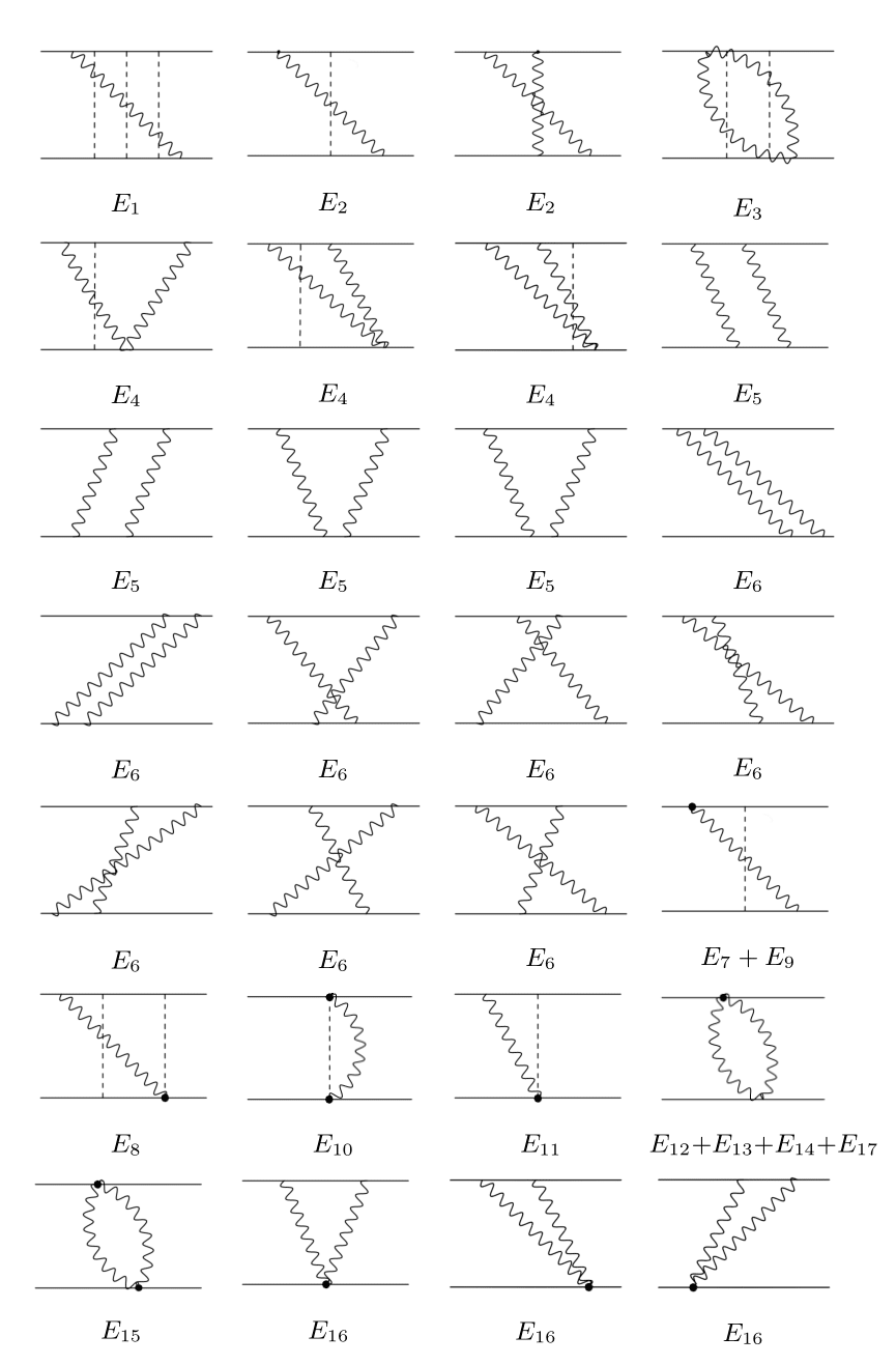
Figure 1: Individual time-ordered diagrams contributing to the middle-energy contribution. We note that $E_{10}$ and $E_{15}$ were calculated from Feynman diagrams. The large dot denotes a correction to the vertex according to $\delta_{\rm ST}H_{\rm FW}$ and $\delta_{\rm DT}H_{\rm FW}$, as explicitly shown in Table I.

where we omitted terms contributing to the fine structure only. From $\delta_{\rm ST}H_{\rm FW}$ and $\delta_{\rm DT}H_{\rm FW}$ in Eqs. (IV) and (32) we obtain the set of all possible vertices that enter time ordered diagrams describing the corrections to the energy of the order $\alpha^{7}\,m$. There are altogether 17 classes of diagrams contributing to the middle-energy contribution, listed in Fig. 1 and in Table. 1. So, the middle-energy contribution $E_{M}$ is split into 17 parts, each of which is represented as an expectation value of the corresponding Hamiltonian,

$$E_{M}=\sum_{i=1}^{17}E_{i}\equiv\sum_{i=1}^{17}\langle\phi|H_{i}|\phi\rangle\,.$$ (33)

In the remaining part of this section we evaluate all diagrams one by one. The calculation is performed in the momentum representation. Most of the terms are calculated from these time-ordered diagrams, for which one can use the following formulas for $\vec{A}$ and $\vec{E}$ in the vertices (IV) and (32)

$$\vec{A}= \ \int\frac{d^{d}k}{\sqrt{(2\,\pi)^{d}}}\frac{1}{\sqrt{2\,k}}\,\vec{\epsilon}_{\lambda}\,\bigl{(}a_{\vec{k},\lambda}\,e^{i\,\vec{k}\,\vec{r}}+a^{+}_{\vec{k},\lambda}\,e^{-i\,\vec{k}\,\vec{r}}\bigr{)}\,,$$ (34)

$$\vec{E}= \ \int\frac{d^{d}k}{\sqrt{(2\,\pi)^{d}}}\frac{k}{\sqrt{2}}\,\vec{\epsilon}_{\lambda}\,i\,\bigl{(}a_{\vec{k},\lambda}\,e^{i\,\vec{k}\,\vec{r}}-a^{+}_{\vec{k},\lambda}\,e^{-i\,\vec{k}\,\vec{r}}\bigr{)}\,,$$ (35)

with $\vec{\epsilon}_{\lambda}$ being the polarization vector and $a_{\vec{k},\lambda}$ and $a^{+}_{\vec{k},\lambda}$ being the annihilation and creation operators, respectively. However, $E_{10}$ and $E_{15}$, due to their specific structure, are calculated from Feynman diagrams. In the following derivation we will extensively use the currents

$$j^{i}(\vec{k})= \ \frac{p^{i}}{m}+\frac{i}{2\,m}\,k^{k}\,\sigma^{ki}\,.$$ (36)

The commutator of two currents with $e^{i\,\vec{k}\,\vec{r}}$ factor is evaluated as

$$[j^{i}(\vec{k}_{1})\,e^{i\,\vec{k}_{1}\,\vec{r}}\,,\,j^{j}(\vec{k}_{2})\,e^{i\,\vec{k}_{2}\,\vec{r}}]= \ \Big{(}j_{n}^{ij}(\vec{p},\vec{k}_{1},\vec{k}_{2})+j_{s}^{ij}(\vec{k}_{1},\vec{k}_{2})\Big{)}\,e^{i\,(\vec{k}_{1}+\vec{k}_{2})\vec{r}}\,,$$ (37)

where

$$j_{n}^{ij}(\vec{p},\vec{k}_{1},\vec{k}_{2})= \ \frac{1}{m^{2}}\big{(}-p^{i}\,k_{1}^{j}+p^{j}\,k_{2}^{i}\big{)}\,,$$ (38)

$$j_{s}^{ij}(\vec{k}_{1},\vec{k}_{2})= \ \frac{i\,\sigma^{ab}}{2\,m^{2}}\,j_{s}^{ij,ab}(\vec{k}_{1},\vec{k}_{2})\,,$$ (39)

$$j_{s}^{ij,ab}(\vec{k}_{1},\vec{k}_{2})= \ -\vec{k}_{1}\cdot\vec{k}_{2}\,\delta^{ia}\,\delta^{jb}-\delta^{ij}k_{1}^{a}k_{2}^{b}+k_{1}^{j}k_{2}^{b}\,\delta^{ia}+k_{1}^{a}k_{2}^{i}\,\delta^{jb}-k_{1}^{j}k_{1}^{a}\,\delta^{ib}-k_{2}^{i}k_{2}^{b}\,\delta^{ja}\,.$$ (40)

Moreover, we will often suppress writing arguments of currents $j_{n}^{ij}(\vec{p},\vec{k}_{1},\vec{k}_{2})$ and $j_{s}^{ij}(\vec{k}_{1},\vec{k}_{2})$.

Table 1: List of 17 diagrams contributing to the middle-energy part $E_{M}$. The exponent in $(H-E)^{n}$ corresponds to the retardation order, i.e., the order in the large-$k$ expansion of $1/(E-H-k)$. The term $E_{5}$ and a part of $E_{6}$ are contained in $E_{2}$ (the transverse photon exchange combined with the Breit interaction) and thus are excluded in order to avoid the double counting. Terms $E_{1}$, a part of $E_{2}$, and terms $E_{7}-E_{11}$ are due to the single transverse photon exchange; the remaining terms correspond to the double transverse photon exchange.

vertex	vertex	vertex/comment	retardation order	diagram
$-\frac{e}{m}\Bigl{(}\vec{p}\cdot\vec{A}+\frac{1}{4}\sigma\cdot B\Bigr{)}$	$-\frac{e}{m}\Bigl{(}\vec{p}\cdot\vec{A}+\frac{1}{4}\sigma\cdot B\Bigr{)}$		$(H-E)^{3}$	$E_{1}$
$-\frac{e}{m}\Bigl{(}\vec{p}\cdot\vec{A}+\frac{1}{4}\sigma\cdot B\Bigr{)}$	$-\frac{e}{m}\Bigl{(}\vec{p}\cdot\vec{A}+\frac{1}{4}\sigma\cdot B\Bigr{)}$	$\mbox{\rm perturbed by}\,H^{(4)}$	$(H-E)$	$E_{2}$
$\frac{e^{2}}{2m}\vec{A}\,{}^{2}$	$\frac{e^{2}}{2m}\vec{A}\,{}^{2}$		$(H-E)^{2}$	$E_{3}$
$\frac{e^{2}}{2m}\vec{A}\,{}^{2}$	$-\frac{e}{m}\Bigl{(}\vec{p}\cdot\vec{A}+\frac{1}{4}\sigma\cdot B\Bigr{)}$	$-\frac{e}{m}\Bigl{(}\vec{p}\cdot\vec{A}+\frac{1}{4}\sigma\cdot B\Bigr{)}$	$(H-E)$	$E_{4}$
$-\frac{e}{m}\Bigl{(}\vec{p}\cdot\vec{A}+\frac{1}{4}\sigma\cdot B\Bigr{)}$	$-\frac{e}{m}\Bigl{(}\vec{p}\cdot\vec{A}+\frac{1}{4}\sigma\cdot B\Bigr{)}$	$\times 2:\,\mbox{\rm reducible part}$	$(H-E)^{0}$	$E_{5}$
$-\frac{e}{m}\Bigl{(}\vec{p}\cdot\vec{A}+\frac{1}{4}\sigma\cdot B\Bigr{)}$	$-\frac{e}{m}\Bigl{(}\vec{p}\cdot\vec{A}+\frac{1}{4}\sigma\cdot B\Bigr{)}$	$\times 2:\,\mbox{\rm irreducible part}$	$(H-E)^{0}$	$E_{6}$
$-\frac{e}{m}\Bigl{(}\vec{p}\cdot\vec{A}+\frac{1}{4}\sigma\cdot B\Bigr{)}$	$\frac{e}{4m^{3}}\bigl{\{}\vec{p}\,{}^{2},\vec{p}\cdot\vec{A}+\frac{1}{4}\,\sigma\cdot B\bigr{\}}$		$(H-E)$	$E_{7}$
$-\frac{e}{m}\Bigl{(}\vec{p}\cdot\vec{A}+\frac{1}{4}\sigma\cdot B\Bigr{)}$	$\frac{e^{2}}{2m^{2}}\sigma^{ij}{E}_{\parallel}^{i}A^{j}$		$(H-E)$	$E_{8}$
$-\frac{e}{m}\Bigl{(}\vec{p}\cdot\vec{A}+\frac{1}{4}\sigma\cdot B\Bigr{)}$	$\frac{ie}{16m^{3}}[\sigma^{ij}\{A^{i},p^{j}\},p^{2}]$		$(H-E)$	$E_{9}$
$\frac{e}{2m^{2}}\sigma^{ij}{E}_{\parallel}^{i}A^{j}$	$\frac{e}{2m^{2}}\sigma^{ij}{E}_{\parallel}^{i}A^{j}$		$(H-E)^{0}$	$E_{10}$
$-\frac{e}{m}\Bigl{(}\vec{p}\cdot\vec{A}+\frac{1}{4}\sigma\cdot B\Bigr{)}$	$\frac{e^{2}}{4\,m^{3}}\,\vec{E}_{\parallel}\,\vec{E}_{\perp}$		$(H-E)^{0}$	$E_{11}$
$\frac{e^{2}}{2m}\vec{A}\,{}^{2}$	$-\frac{1}{8m^{3}}\{\,\vec{p}\,{}^{2},e^{2}\vec{A}\,{}^{2}\}$		$(H-E)^{0}$	$E_{12}$
$\frac{e^{2}}{2m}\vec{A}\,{}^{2}$	$\frac{e^{2}}{2m^{3}}(\vec{A}\cdot\vec{p}\,)^{2}$		$(H-E)^{0}$	$E_{12}$
$\frac{e^{2}}{2m}\vec{A}\,{}^{2}$	$\frac{e^{2}}{8m^{3}}\vec{E}^{2}_{\perp}$		$(H-E)^{0}$	$E_{13}$
$\frac{e^{2}}{2m}\vec{A}\,{}^{2}$	$-\frac{e^{2}}{16m^{3}}B^{ij}B^{ij}$		$(H-E)^{0}$	$E_{14}$
$\frac{1}{4m^{2}}e^{2}\,\sigma^{ij}{E}_{\perp}^{i}A^{j}$	$\frac{1}{4m^{2}}e^{2}\,\sigma^{ij}{E}_{\perp}^{i}A^{j}$		$(H-E)^{0}$	$E_{15}$
$\frac{1}{4m^{2}}e^{2}\,\sigma^{ij}E_{\perp}^{i}A^{j}$	$-\frac{e}{m}\Bigl{(}\vec{p}\cdot\vec{A}+\frac{1}{4}\sigma\cdot B\Bigr{)}$	$-\frac{e}{m}\Bigl{(}\vec{p}\cdot\vec{A}+\frac{1}{4}\sigma\cdot B\Bigr{)}$	$(H-E)^{0}$	$E_{16}$
$\frac{e^{2}}{2m}\vec{A}\,{}^{2}$	$-\frac{e^{2}}{8m^{3}}A^{i}\,\nabla^{j}B^{ij}$		$(H-E)^{0}$	$E_{17}$

IV.1 Evaluation of individual diagrams

IV.1.1 Triple retardation in nonrelativistic single transverse photon exchange $E_{1}$

The correction due to the single transverse photon exchange reads

$$\delta E=e^{2}\int\frac{d^{d}k}{(2\pi)^{d}\,2k}\delta_{\perp}^{ij}(k)\langle\phi|j_{1}^{i}(k)e^{i\vec{k}\cdot\vec{r}_{1}}\,\frac{1}{E_{0}-H_{0}-k}\,j_{2}^{j}(-k)e^{-i\vec{k}\cdot\vec{r}_{2}}|\phi\rangle+(1\leftrightarrow 2)\,.$$ (41)

Expanding the denominator of the above expression in $k$ and taking only the term contributing to the order $m\alpha^{7}$, we obtain

$$E_{1}= \ e^{2}\int\frac{d^{d}k}{(2\pi)^{d}\,2k^{5}}\delta_{\perp}^{ij}(k)\langle\phi|\biggl{(}\frac{p_{1}^{i}}{m}+\frac{1}{2m}\sigma_{1}^{ki}\nabla_{1}^{k}\biggr{)}e^{i\vec{k}\cdot\vec{r}_{1}}(H_{0}-E_{0})^{3}\biggl{(}\frac{p_{2}^{j}}{m}+\frac{1}{2m}\sigma_{2}^{lj}\nabla_{2}^{l}\biggr{)}e^{-i\vec{k}\cdot\vec{r}_{2}}|\phi\rangle+(1\leftrightarrow 2)$$

$$= \ E_{1}^{ss}+E_{1}^{nn}\,,$$ (42)

where

$$E_{1}^{ss} = \frac{e^{2}}{2\,m^{2}}\int\frac{d^{d}k}{(2\pi)^{d}\,k^{5}}\delta_{\perp}^{ij}(k)\langle\phi|\biggl{[}\biggl{[}\frac{i}{2m}\sigma_{1}^{ki}k^{k}\,e^{i\vec{k}\cdot\vec{r}_{1}},H_{0}-E_{0}\biggr{]},\biggl{[}H_{0}-E_{0},\biggl{[}H_{0}-E_{0},\frac{(-i)}{2m}\sigma_{2}^{lj}k^{l}\,e^{-i\vec{k}\cdot\vec{r}_{2}}\biggr{]}\biggr{]}\biggr{]}|\phi\rangle$$ (43)

$$= \frac{e^{2}}{8\,m^{4}}\,\frac{\sigma_{1}\cdot\sigma_{2}}{d}\int\frac{d^{d}k}{(2\pi)^{d}\,k^{3}}\,k^{m}k^{n}\langle\phi|\,e^{i\vec{k}\cdot\vec{r}}\,\biggl{[}p_{1}^{n},\biggl{[}\biggl{[}\frac{\alpha}{r}\biggr{]}_{\epsilon},p_{2}^{m}\biggr{]}\biggr{]}|\phi\rangle\,,$$

$$E_{1}^{nn} = \frac{e^{2}}{2\,m^{2}}\int\frac{d^{d}k}{(2\pi)^{d}k^{5}}\delta_{\perp}^{ij}(k)\langle\phi|\bigl{[}\bigl{[}\,p_{1}^{i}\,e^{i\vec{k}\cdot\vec{r}_{1}},H_{0}-E_{0}\bigr{]},\bigl{[}H_{0}-E_{0},\bigl{[}H_{0}-E_{0},p_{2}^{j}\,e^{-i\vec{k}\cdot\vec{r}_{2}}\bigr{]}\bigr{]}\bigr{]}|\phi\rangle$$ (44)

$$= \frac{e^{2}}{2\,m^{2}}\int\frac{d^{d}k}{(2\pi)^{d}k^{5}}\delta_{\perp}^{ij}(k)\Bigl{\langle}\phi\Bigl{|}\Bigl{[}\Bigl{[}\,p_{1}^{i}\,e^{i\vec{k}\cdot\vec{r}_{1}},\frac{p_{1}^{2}}{2\,m}+V\Bigr{]},\Bigl{[}\frac{p_{1}^{2}}{2\,m}+\frac{p_{2}^{2}}{2\,m}+V,\Bigl{[}\frac{p_{2}^{2}}{2\,m}+V,p_{2}^{j}\,e^{-i\vec{k}\cdot\vec{r}_{2}}\Bigr{]}\Bigr{]}\Bigr{]}\Bigr{|}\phi\Bigr{\rangle}\,.$$

The spin part is easy to evaluate and for this we use integrals from Appendix C with the result

$$H_{1}^{ss}=\frac{\alpha^{2}}{m^{4}}\,\sigma_{1}\cdot\sigma_{2}\,\Big{(}-\frac{1}{3}-\frac{1}{9\epsilon}+\frac{2}{9}\ln 2+\frac{2}{9}\ln q\Big{)}\,q^{2}.$$ (45)

For the spin-independent part $H_{1}^{nn}$ the evaluation is quite lengthy and thus is moved to Appendix F. The result for the sum of both parts is

$$H_{1} = \frac{\alpha^{2}}{m^{4}}\bigg{\{}\sigma_{1}\cdot\sigma_{2}\,\Big{(}-\frac{1}{3}-\frac{1}{9\epsilon}+\frac{2}{9}\ln 2+\frac{2}{9}\ln q\Big{)}\,q^{2}+\frac{4}{45}\big{(}\vec{P}_{1}-\vec{P}_{2}\big{)}^{2}-\frac{26}{15}\frac{\big{[}\big{(}\vec{P}_{1}-\vec{P}_{2}\big{)}\cdot\vec{q}\big{]}^{2}}{q^{2}}+\frac{28}{45}q^{2}+\frac{4}{9}\vec{P}_{1}\cdot\vec{P}_{2}$$ (46)

$$-\frac{16}{3}\frac{\big{(}\vec{P}_{1}\cdot\vec{q}\big{)}\big{(}\vec{P}_{2}\cdot\vec{q}\big{)}}{q^{2}}+\bigg{(}\frac{8}{15}\big{(}\vec{P}_{1}-\vec{P}_{2}\big{)}^{2}+\frac{4}{3}\frac{\big{[}\big{(}\vec{P}_{1}-\vec{P}_{2}\big{)}\cdot\vec{q}\big{]}^{2}}{q^{2}}-\frac{16}{15}q^{2}+\frac{8}{3}\frac{\big{(}\vec{P}_{1}\cdot\vec{q}\big{)}\big{(}\vec{P}_{2}\cdot\vec{q}\big{)}}{q^{2}}\bigg{)}\bigg{(}-\frac{1}{2\epsilon}+\ln 2+\ln q\bigg{)}\bigg{\}}$$

$$+\frac{\pi\alpha^{3}}{m^{3}}\bigg{(}-\frac{2}{5}+\frac{1}{15\epsilon}-\frac{4}{15}\ln q\bigg{)}\,q+\frac{\alpha^{3}}{m^{3}}\bigg{\{}\bigg{[}p_{2}^{j},-\bigg{[}\frac{Z}{r_{2}}\bigg{]}_{\epsilon}\bigg{]}\,\bigg{(}-\frac{2}{15}+\frac{14}{15\epsilon}-\frac{28}{15}\ln 2-\frac{28}{15}\ln q\bigg{)}\frac{q^{j}}{q^{2}}$$

$$+\bigg{[}\bigg{[}p_{2}^{i},-\bigg{[}\frac{Z}{r_{2}}\bigg{]}_{\epsilon}\bigg{]},p_{2}^{j}\bigg{]}\bigg{[}\delta^{ij}\bigg{(}-\frac{4}{5}-\frac{4}{15\epsilon}+\frac{8}{15}\ln 2+\frac{8}{15}\ln q\bigg{)}+\frac{q^{i}q^{j}}{q^{2}}\bigg{(}\frac{16}{15}+\frac{16}{15\epsilon}-\frac{32}{15}\ln 2-\frac{32}{15}\ln q\bigg{)}\bigg{]}\frac{1}{q^{2}}$$

$$+(1\leftrightarrow 2)\bigg{\}}\,.$$

IV.1.2 Single transverse photon exchange with Breit correction $E_{2}$

This contribution comes from the perturbation of the nonrelativistic Hamiltonian $H_{0}$, energy $E_{0}$ and wave function $\phi$ by the Breit Hamiltonian $H^{(4)}$ in the single transverse photon exchange. We thus have

$$E_{2}= \ e^{2}\int\frac{d^{d}k}{(2\pi)^{d}\,2k^{3}}\delta_{\perp}^{ij}(k)\,\delta\langle\phi|\biggl{(}\frac{p_{1}^{i}}{m}+\frac{1}{2m}\sigma_{1}^{ki}\nabla_{1}^{k}\biggr{)}e^{i\vec{k}\cdot\vec{r}_{1}}(H-E)\biggl{(}\frac{p_{2}^{j}}{m}+\frac{1}{2m}\sigma_{2}^{lj}\nabla_{2}^{l}\biggr{)}e^{-i\vec{k}\cdot\vec{r}_{2}}|\phi\rangle+(1\leftrightarrow 2)$$

$$= \ e^{2}\int\frac{d^{d}k}{(2\pi)^{d}\,2k^{3}}\delta_{\perp}^{ij}(k)\,\delta\langle\phi|\biggl{[}\biggl{(}\frac{p_{1}^{i}}{m}+\frac{1}{2m}\sigma_{1}^{ki}\nabla_{1}^{k}\biggr{)}e^{i\vec{k}\cdot\vec{r}_{1}},\biggl{[}H-E,\biggl{(}\frac{p_{2}^{j}}{m}+\frac{1}{2m}\sigma_{2}^{lj}\nabla_{2}^{l}\biggr{)}e^{-i\vec{k}\cdot\vec{r}_{2}}\biggr{]}\biggr{]}|\phi\rangle$$

$$= \ e^{2}\int\frac{d^{d}k}{(2\pi)^{d}\,2k^{3}}\delta_{\perp}^{ij}(k)\biggl{\{}\langle\phi|\biggl{[}\biggl{(}\frac{p_{1}^{i}}{m}+\frac{1}{2m}\sigma_{1}^{ki}\nabla_{1}^{k}\biggr{)}e^{i\vec{k}\cdot\vec{r}_{1}},\biggl{[}H^{(4)}-E^{(4)},\biggl{(}\frac{p_{2}^{j}}{m}+\frac{1}{2m}\sigma_{2}^{lj}\nabla_{2}^{l}\biggr{)}e^{-i\vec{k}\cdot\vec{r}_{2}}\biggr{]}\biggr{]}|\phi\rangle$$

$$+\,\langle\phi|H^{(4)}\,\frac{1}{(E_{0}-H_{0})^{\prime}}\biggl{[}\biggl{(}\frac{p_{1}^{i}}{m}+\frac{1}{2m}\sigma_{1}^{ki}\nabla_{1}^{k}\biggr{)}e^{i\vec{k}\cdot\vec{r}_{1}},\biggl{[}H_{0}-E_{0},\biggl{(}\frac{p_{2}^{j}}{m}+\frac{1}{2m}\sigma_{2}^{lj}\nabla_{2}^{l}\biggr{)}e^{-i\vec{k}\cdot\vec{r}_{2}}\biggr{]}\biggr{]}|\phi\rangle$$

$$+\,\langle\phi|\biggl{[}\biggl{(}\frac{p_{1}^{i}}{m}+\frac{1}{2m}\sigma_{1}^{ki}\nabla_{1}^{k}\biggr{)}e^{i\vec{k}\cdot\vec{r}_{1}},\biggl{[}H_{0}-E_{0},\biggl{(}\frac{p_{2}^{j}}{m}+\frac{1}{2m}\sigma_{2}^{lj}\nabla_{2}^{l}\biggr{)}e^{-i\vec{k}\cdot\vec{r}_{2}}\biggr{]}\biggr{]}\,\frac{1}{(E_{0}-H_{0})^{\prime}}\,H^{(4)}|\phi\rangle\biggr{\}}\,.$$ (47)

The last two lines are a part of the second-order contribution, the third term of Eq. (5) and thus will be omitted here, so

$$E_{2} = e^{2}\int\frac{d^{d}k}{(2\pi)^{d}\,2k^{3}}\delta_{\perp}^{ij}(k)\langle\phi|\biggl{[}\biggl{(}\frac{p_{1}^{i}}{m}+\frac{1}{2m}\sigma_{1}^{ki}\nabla_{1}^{k}\biggr{)}\,e^{i\vec{k}\cdot\vec{r}_{1}},\biggl{[}H^{(4)}-E^{(4)},\biggl{(}\frac{p_{2}^{j}}{m}+\frac{1}{2m}\sigma_{2}^{lj}\nabla_{2}^{l}\biggr{)}\,e^{-i\vec{k}\cdot\vec{r}_{2}}\biggr{]}\biggr{]}|\phi\rangle$$ (48)

$$= E^{\prime}_{2}+E^{\prime\prime}_{2}\,,$$ (49)

where $E^{\prime}_{2}$ is a correction due to $H^{\prime(4)}$ and $E^{\prime\prime}_{2}$ is due to $H^{\prime\prime(4)}$. $E^{\prime\prime}_{2}$ is the double transverse photon exchange, because $H^{\prime\prime(4)}$ comes from the transverse photon exchange. Therefore, this double transverse photon exchange will later be excluded from $E_{5}+E^{\prime\prime}_{6}$ in Eq. (80), to avoid double counting. We transform $E^{\prime}_{2}$ and $E^{\prime\prime}_{2}$ as

$$E^{\prime}_{2}= \ e^{2}\int\frac{d^{d}k}{(2\pi)^{d}\,2k^{3}}\delta_{\perp}^{ij}(k)\frac{1}{m^{4}}\biggl{\langle}\phi\biggl{|}-\frac{\sigma_{1}^{ki}\,\sigma_{1}^{mn}}{8}\,k^{k}\,k^{n}\,e^{i\vec{k}\cdot\vec{r}}\,\nabla^{j}\,\nabla^{m}\biggl{[}\frac{\alpha}{r}\biggr{]}_{\epsilon}-\frac{\sigma_{2}^{mn}\,\sigma_{2}^{lj}}{8}\,k^{l}\,k^{n}\,e^{i\vec{k}\cdot\vec{r}}\,\nabla^{i}\,\nabla^{m}\biggl{[}\frac{\alpha}{r}\biggr{]}_{\epsilon}$$

$$\ +\bigl{[}p_{1}^{i}\,e^{i\vec{k}\cdot\vec{r}_{1}},\bigl{[}-\pi\,\alpha\,\delta^{d}(r)\,,\,p_{2}^{j}\,e^{-i\vec{k}\cdot\vec{r}_{2}}\bigr{]}\bigr{]}\biggr{|}\phi\biggr{\rangle}\,,$$ (50)

$$E^{\prime\prime}_{2}= \ -e^{4}\int\frac{d^{d}k_{1}}{(2\pi)^{d}\,2k_{1}^{3}}\int\frac{d^{d}k_{2}}{(2\pi)^{d}\,k_{2}^{2}}\delta_{\perp}^{ij}(k_{1})\delta_{\perp}^{mn}(k_{2})\langle\phi|\bigl{[}j_{1}^{i}\,e^{i\vec{k_{1}}\cdot\vec{r}_{1}},j_{1}^{m}\,e^{i\vec{k_{2}}\cdot\vec{r}_{1}}\bigr{]}\bigl{[}j_{2}^{n}\,e^{-i\vec{k_{2}}\cdot\vec{r}_{2}},j_{2}^{j}\,e^{-i\vec{k_{1}}\cdot\vec{r}_{2}}\bigr{]}|\phi\rangle\,.$$ (51)

We now evaluate the $E_{2}^{\prime}$ part. The term with the delta function vanishes because, due to the delta function, the exponent function disappears, $e^{i\vec{k}\cdot\vec{r}}=1$, and in the dimensional regularization, by definition,

$$\int d^{d}k\,k^{\alpha}=0\,.$$ (52)

We thus have

$$E_{2}^{\prime}= \ -\frac{e^{2}}{m^{4}}\int\frac{d^{d}k}{(2\pi)^{d}\,2k^{3}}\delta_{\perp}^{ij}(k)\biggl{\langle}\phi\biggl{|}\frac{\sigma_{1}^{ki}\,\sigma_{1}^{mn}}{8}\,k^{k}\,k^{n}\,e^{i\vec{k}\cdot\vec{r}}\,\nabla^{j}\,\nabla^{m}\biggl{[}\frac{\alpha}{r}\biggr{]}_{\epsilon}+\frac{\sigma_{2}^{mn}\,\sigma_{2}^{lj}}{8}\,k^{l}\,k^{n}\,e^{i\vec{k}\cdot\vec{r}}\,\nabla^{i}\,\nabla^{m}\biggl{[}\frac{\alpha}{r}\biggr{]}_{\epsilon}\biggr{|}\phi\biggr{\rangle}$$

$$= \ \frac{e^{2}}{4m^{4}}\int\frac{d^{d}k}{(2\pi)^{d}\,2k}\delta_{\perp}^{ij}(k)\biggl{\langle}\phi\biggl{|}\,e^{i\vec{k}\cdot\vec{r}}\,\nabla^{j}\,\nabla^{i}\biggl{[}\frac{\alpha}{r}\biggr{]}_{\epsilon}\biggr{|}\phi\biggr{\rangle}\,.$$ (53)

The corresponding operator in the momentum representation is

$$H_{2}^{\prime}=\frac{\alpha^{2}}{m^{4}}\biggl{(}-\frac{7}{9}-\frac{1}{3\epsilon}+\frac{2}{3}\ln 2+\frac{2}{3}\ln q^{2}\biggr{)}q^{2}\,.$$ (54)

Now we turn to contributions due to $E_{2}^{\prime\prime}$ and use Eq. (37),

$$E_{2}^{\prime\prime} = e^{4}\int\frac{d^{d}k_{1}}{(2\pi)^{d}\,2k_{1}^{3}}\int\frac{d^{d}k_{2}}{(2\pi)^{d}\,k_{2}^{2}}\delta_{\perp}^{ij}(k_{1})\delta_{\perp}^{mn}(k_{2})\langle\phi|j_{n}^{im}j_{n}^{jn}+j_{s}^{im,ab}j_{s}^{jn,kl}\,\sigma_{1}^{ab}\sigma_{2}^{kl}|\phi\rangle\,.$$ (55)

This can be spin averaged with the help of Eq. (188). The corresponding operator in the momentum representation is

$$H_{2}^{\prime\prime}=\frac{\alpha^{2}}{m^{4}}\bigg{(}-\frac{8}{3}\vec{P}_{1}\cdot\vec{P}_{2}+\frac{8}{3}\frac{\big{(}\vec{P}_{1}\cdot\vec{q}\big{)}\big{(}\vec{P}_{2}\cdot\vec{q}\big{)}}{q^{2}}\bigg{)}\bigg{(}\frac{1}{2}-\frac{1}{2\epsilon}+\ln 2+\ln q\biggr{)}+\frac{\alpha^{2}}{m^{4}}\sigma_{1}\cdot\sigma_{2}\biggl{(}-\frac{10}{9}-\frac{5}{18\epsilon}+\frac{5}{9}\ln 2+\frac{5}{9}\ln q\biggr{)}\,q\,,$$ (56)

and the result for $H_{2}=H_{2}^{\prime}+H_{2}^{\prime\prime}$ is then

$$H_{2} = \frac{\alpha^{2}}{m^{4}}\bigg{\{}\sigma_{1}\cdot\sigma_{2}\biggl{(}-\frac{10}{9}-\frac{5}{18\epsilon}+\frac{5}{9}\ln 2+\frac{5}{9}\ln q\biggr{)}\,q^{2}+\biggl{(}-\frac{7}{9}-\frac{1}{3\epsilon}+\frac{2}{3}\ln 2+\frac{2}{3}\ln q^{2}\biggr{)}q^{2}\bigg{\}}$$ (57)

$$+\frac{\alpha^{2}}{m^{4}}\bigg{(}-\frac{8}{3}\vec{P}_{1}\cdot\vec{P}_{2}+\frac{8}{3}\frac{\big{(}\vec{P}_{1}\cdot\vec{q}\big{)}\big{(}\vec{P}_{2}\cdot\vec{q}\big{)}}{q^{2}}\bigg{)}\bigg{(}\frac{1}{2}-\frac{1}{2\epsilon}+\ln 2+\ln q\biggr{)}\,.$$

IV.1.3 Retardation in the double seagull $E_{3}$

In the case of the double seagull diagram we have to take the double retardation to obtain correction of the order $m\alpha^{7}$,

$$E_{3} = \biggl{(}\frac{e^{2}}{2m}\biggr{)}^{2}\,2\int\frac{d^{d}k_{1}}{(2\pi)^{d}\,2k_{1}}\int\frac{d^{d}k_{2}}{(2\pi)^{d}\,2k_{2}}\delta_{\perp}^{ij}(k_{1})\delta_{\perp}^{ij}(k_{2})\langle\phi|e^{i(\vec{k}_{1}+\vec{k}_{2})\cdot\vec{r}_{1}}\,\frac{1}{E_{0}-H_{0}-k_{1}-k_{2}}\,e^{-i(\vec{k}_{1}+\vec{k}_{2})\cdot\vec{r}_{2}}|\phi\rangle+(1\leftrightarrow 2)$$ (58)

$$\approx -\biggl{(}\frac{e^{2}}{2m}\biggr{)}^{2}\,2\int\frac{d^{d}k_{1}}{(2\pi)^{d}\,2k_{1}}\int\frac{d^{d}k_{2}}{(2\pi)^{d}\,2k_{2}}\delta_{\perp}^{ij}(k_{1})\delta_{\perp}^{ij}(k_{2})\langle\phi|e^{i(\vec{k}_{1}+\vec{k}_{2})\cdot\vec{r}_{1}}\,\frac{(H_{0}-E_{0})^{2}}{(k_{1}+k_{2})^{3}}\,e^{-i(\vec{k}_{1}+\vec{k}_{2})\cdot\vec{r}_{2}}|\phi\rangle+(1\leftrightarrow 2)$$

$$= -\Big{(}\frac{e^{2}}{2m}\Big{)}^{2}\int\frac{d^{d}k_{1}}{(2\pi)^{d}\,k_{1}}\int\frac{d^{d}k_{2}}{(2\pi)^{d}\,k_{2}}\frac{1}{(k_{1}+k_{2})^{3}}\delta_{\perp}^{ij}(k_{1})\delta_{\perp}^{ij}(k_{2})\bigg{\langle}\phi\bigg{|}\bigg{[}\frac{p_{2}^{2}}{2m},\bigg{[}e^{i(\vec{k}_{1}+\vec{k}_{2})\cdot\vec{r}},\frac{p_{1}^{2}}{2m}\bigg{]}\bigg{]}\bigg{|}\phi\bigg{\rangle}\,.$$

The result in momentum representation is

$$H_{3} = \frac{\alpha^{2}}{m^{4}}\,\frac{(-9+8\ln 2)}{5}\frac{(\vec{P}_{1}\cdot\vec{q})(\vec{P}_{2}\cdot\vec{q})}{q^{2}}\,.$$ (59)

IV.1.4 Retardation in the single seagull $E_{4}$

For the single seagull diagram we have to take a single retardation correction in order to obtain the contribution of the order $m\alpha^{7}$. Using the definition of $j_{1}^{i}(k)$, we write $E_{4}$ as

$$E_{4} = \frac{e^{4}}{m}\,\int\frac{d^{d}k_{1}}{(2\pi)^{d}\,2k_{1}}\int\frac{d^{d}k_{2}}{(2\pi)^{d}\,2k_{2}}\delta_{\perp}^{in}(k_{1})\delta_{\perp}^{im}(k_{2})$$ (60)

$$\times\biggl{\{}\langle\phi|j_{1}^{n}(k_{1})\,e^{i\vec{k}_{1}\cdot\vec{r}_{1}}\,\frac{1}{E_{0}-H_{0}-k_{1}}\,e^{-i(\vec{k}_{1}+\vec{k}_{2})\cdot\vec{r}_{2}}\,\frac{1}{E_{0}-H_{0}-k_{2}}\,j_{1}^{m}(k_{2})\,e^{i\vec{k}_{2}\cdot\vec{r}_{1}}|\phi\rangle$$

$$+\,\langle\phi|j_{1}^{n}(k_{1})\,e^{i\vec{k}_{1}\cdot\vec{r}_{1}}\,\frac{1}{E_{0}-H_{0}-k_{1}}\,j_{1}^{m}(k_{2})\,e^{i\vec{k}_{2}\cdot\vec{r}_{1}}\,\frac{1}{E_{0}-H_{0}-k_{1}-k_{2}}\,e^{-i(\vec{k}_{1}+\vec{k}_{2})\cdot\vec{r}_{2}}|\phi\rangle$$

$$+\,\langle\phi|e^{-i(\vec{k}_{1}+\vec{k}_{2})\cdot\vec{r}_{2}}\,\frac{1}{E_{0}-H_{0}-k_{1}-k_{2}}\,j_{1}^{n}(k_{1})\,e^{i\vec{k}_{1}\cdot\vec{r}_{1}}\,\frac{1}{E_{0}-H_{0}-k_{2}}\,j_{1}^{m}(k_{2})\,e^{i\vec{k}_{2}\cdot\vec{r}_{1}}|\phi\rangle\biggr{\}}+(1\leftrightarrow 2)\,.$$

After expanding in $H_{0}-E_{0}$ and further simplifications of the expression, it can be transformed to

$$E_{4} = -\frac{e^{4}}{m}\,\int\frac{d^{d}k_{1}}{(2\pi)^{d}\,2k_{1}}\int\frac{d^{d}k_{2}}{(2\pi)^{d}\,2k_{2}}\delta_{\perp}^{in}(k_{1})\delta_{\perp}^{im}(k_{2})$$ (61)

$$\times\biggl{\{}\frac{1}{k_{1}^{2}}\,\Bigl{(}\frac{1}{k_{2}}+\frac{1}{k_{1}+k_{2}}\Bigr{)}\langle\phi|\bigl{[}\bigl{[}j_{1}^{n}(k_{1})\,e^{i\vec{k}_{1}\cdot\vec{r}_{1}}\,,\,H_{0}-E_{0}\bigr{]}\,,\,j_{1}^{m}(k_{2})\,e^{i\vec{k}_{2}\cdot\vec{r}_{1}}\bigr{]}\,e^{-i(\vec{k}_{1}+\vec{k}_{2})\cdot\vec{r}_{2}}|\phi\rangle$$

$$+\frac{1}{k_{1}\,(k_{1}+k_{2})^{2}}\,\langle\phi|\bigl{[}j_{1}^{n}(k_{1})\,e^{i\vec{k}_{1}\cdot\vec{r}_{1}}\,,\,j_{1}^{m}(k_{2})\,e^{i\vec{k}_{2}\cdot\vec{r}_{1}}\bigr{]}\,\bigl{[}H_{0}-E_{0}\,,\,e^{-i(\vec{k}_{1}+\vec{k}_{2})\cdot\vec{r}_{2}}\bigr{]}|\phi\rangle\biggr{\}}+(1\leftrightarrow 2)\,.$$

Using the the Jacobi identity

$$[[A_{1}\,,\,B]\,,\,A_{2}]-[[A_{2}\,,\,B]\,,\,A_{1}]=[[A_{1}\,,\,A_{2}]\,,\,B]\,,$$ (62)

we obtain

$$E_{4}= \ -\frac{e^{4}}{2\,m}\,\int\frac{d^{d}k_{1}}{(2\pi)^{d}\,2k_{1}}\int\frac{d^{d}k_{2}}{(2\pi)^{d}\,2k_{2}}\delta_{\perp}^{in}(k_{1})\delta_{\perp}^{im}(k_{2})$$

$$\times\biggl{\{}\Bigl{(}\frac{1}{k_{1}^{2}\,k_{2}}+\frac{1}{k_{1}\,k_{2}^{2}}+\frac{1}{k_{1}^{2}}\,\frac{1}{k_{1}+k_{2}}+\frac{1}{k_{2}^{2}}\,\frac{1}{k_{1}+k_{2}}\Bigr{)}\langle\phi|\bigl{[}\bigl{[}j_{1}^{n}(k_{1})\,e^{i\vec{k}_{1}\cdot\vec{r}_{1}}\,,\,H_{0}-E_{0}\bigr{]}\,,\,j_{1}^{m}(k_{2})\,e^{i\vec{k}_{2}\cdot\vec{r}_{1}}\bigr{]}\,e^{-i(\vec{k}_{1}+\vec{k}_{2})\cdot\vec{r}_{2}}|\phi\rangle$$

$$\ +\frac{1}{k_{1}^{2}}\,\Bigl{(}\frac{1}{k_{2}}+\frac{1}{k_{1}+k_{2}}+\frac{2\,k_{1}}{(k_{1}+k_{2})^{2}}\Bigr{)}\,\langle\phi|\bigl{[}j_{1}^{n}(k_{1})\,e^{i\vec{k}_{1}\cdot\vec{r}_{1}}\,,\,j_{1}^{m}(k_{2})\,e^{i\vec{k}_{2}\cdot\vec{r}_{1}}\bigr{]}\,\bigl{[}H_{0}-E_{0}\,,\,e^{-i(\vec{k}_{1}+\vec{k}_{2})\cdot\vec{r}_{2}}\bigr{]}|\phi\rangle\biggr{\}}+(1\leftrightarrow 2)$$

$$= \ E_{4,1}+E_{4,2}+E_{4,3}+E_{4,4}\,.$$ (63)

Here, $E_{4,4}$ corresponds to the second term in the curly brackets, while $E_{4,1}$, $E_{4,2}$, and $E_{4,3}$ are parts of the first term in the curly brackets. Specifically, $E_{4,1}$ corresponds to the spin-dependent part, and $E_{4,2}$ and $E_{4,3}$ are coming from the two- and three-photon contributions in the spin-independent part, correspondingly.

We start with the first term in the curly brackets in Eq. (IV.1.4),

$$E_{4,1}+E_{4,2}+E_{4,3} = -\frac{e^{4}}{2\,m^{3}}\int\frac{d^{d}k_{1}}{(2\pi)^{d}\,2\,k_{1}}\int\frac{d^{d}k_{2}}{(2\pi)^{d}\,2\,k_{2}}\Bigl{(}\frac{1}{k_{1}^{2}\,k_{2}}+\frac{1}{k_{1}\,k_{2}^{2}}+\frac{1}{k_{1}^{2}}\,\frac{1}{k_{1}+k_{2}}+\frac{1}{k_{2}^{2}}\,\frac{1}{k_{1}+k_{2}}\Bigr{)}\,\delta^{in}_{\perp}(k_{1})\,\delta^{im}_{\perp}(k_{2})$$ (64)

$$\times\langle\phi|\,\biggl{[}\,e^{-i(\vec{k}_{1}+\vec{k}_{2})\cdot\vec{r}_{2}}\,\biggl{(}p_{1}^{m}+\frac{i}{2}\sigma_{1}^{rm}k_{2}^{r}\biggr{)}\,e^{i\vec{k}_{2}\cdot\vec{r}_{1}},\biggl{[}\,\frac{p_{1}^{2}}{2m}+V,\,\biggl{(}p_{1}^{n}+\frac{i}{2}\sigma_{1}^{sn}k_{1}^{s}\biggr{)}\,e^{i\vec{k}_{1}\cdot\vec{r}_{1}}\biggr{]}\biggr{]}\,|\phi\rangle+(1\leftrightarrow 2)\,.$$

The spin-dependent part $E_{4,1}$ is

$$E_{4,1} = \frac{e^{4}}{16m^{3}}\int\frac{d^{d}k_{1}}{(2\pi)^{d}}\int\frac{d^{d}k_{2}}{(2\pi)^{d}}\frac{1}{k_{1}^{3}k_{2}}\,\Bigl{(}\frac{1}{k_{2}}+\frac{1}{k_{1}+k_{2}}\Bigr{)}\,\delta^{in}_{\perp}(k_{1})\,\delta^{im}_{\perp}(k_{2})\,\sigma_{1}^{rm}\sigma_{1}^{sn}k_{2}^{r}k_{1}^{s}$$ (65)

$$\times\langle\phi|\,e^{-i(\vec{k}_{1}+\vec{k}_{2})\cdot\vec{r}_{2}}\biggl{[}e^{i\vec{k}_{2}\cdot\vec{r}_{1}},\biggl{[}\,\frac{p_{1}^{2}}{2m},e^{i\vec{k}_{1}\cdot\vec{r}_{1}}\biggr{]}\biggr{]}\,|\phi\rangle+(1\leftrightarrow 2)$$

$$= -\frac{e^{4}}{16m^{4}}\int\frac{d^{d}k_{1}}{(2\pi)^{d}}\int\frac{d^{d}k_{2}}{(2\pi)^{d}}\frac{1}{k_{1}^{3}k_{2}}\,\Bigl{(}\frac{1}{k_{2}}+\frac{1}{k_{1}+k_{2}}\Bigr{)}\,\delta^{in}_{\perp}(k_{1})\,\delta^{im}_{\perp}(k_{2})\big{(}\delta^{mn}\big{(}\vec{k}_{1}\cdot\vec{k}_{2}\big{)}^{2}-k_{1}^{m}k_{2}^{n}\,\vec{k}_{1}\cdot\vec{k}_{2}\big{)}\langle\phi|\,e^{i(\vec{k}_{1}+\vec{k}_{2})\cdot\vec{r}}|\phi\rangle$$

$$+(1\leftrightarrow 2)\,,$$

where we performed spin averaging. The result in momentum representation is

$$H_{4,1}=\frac{\alpha^{2}}{m^{4}}\,\Big{(}-\frac{5}{72}+\frac{23}{24\epsilon}-\frac{23}{12}\ln q\Big{)}\,q^{2}\,.$$ (66)

The spin-independent two-photon exchange part is

$$E_{4,2}= \ -\frac{e^{4}}{8\,m^{3}}\int\frac{d^{d}k_{1}}{(2\pi)^{d}}\int\frac{d^{d}k_{2}}{(2\pi)^{d}}\,\frac{1}{k_{1}\,k_{2}}\Bigl{(}\frac{1}{k_{1}^{2}\,k_{2}}+\frac{1}{k_{1}\,k_{2}^{2}}+\frac{1}{k_{1}^{2}}\,\frac{1}{k_{1}+k_{2}}+\frac{1}{k_{2}^{2}}\,\frac{1}{k_{1}+k_{2}}\Bigr{)}\,\delta^{in}_{\perp}(k_{1})\,\delta^{im}_{\perp}(k_{2})$$

$$\times\langle\phi|\,\biggl{[}\,e^{-i(\vec{k}_{1}+\vec{k}_{2})\cdot\vec{r}_{2}}\,p_{1}^{m}\,e^{i\vec{k}_{2}\cdot\vec{r}_{1}},\biggl{[}\,\frac{p_{1}^{2}}{2m},\,p_{1}^{n}\,e^{i\vec{k}_{1}\cdot\vec{r}_{1}}\biggr{]}\biggr{]}\,|\phi\rangle+(1\leftrightarrow 2)$$

$$= \ -\frac{e^{4}}{8\,m^{4}}\int\frac{d^{d}k_{1}}{(2\pi)^{d}}\int\frac{d^{d}k_{2}}{(2\pi)^{d}}\frac{1}{k_{1}^{3}k_{2}}\,\Bigl{(}\frac{1}{k_{2}}+\frac{1}{k_{1}+k_{2}}\Bigr{)}\langle\phi|\,p_{1}^{m}\biggl{(}-2\,\vec{k}_{1}\cdot\vec{k}_{2}\,\delta_{\perp}^{in}(k_{1})\,\delta_{\perp}^{im}(k_{2})$$

$$-(k_{1}^{n}-k_{2}^{n})\,k_{2}^{k}\,\delta_{\perp}^{ik}(k_{1})\delta_{\perp}^{im}(k_{2})+(k_{1}^{m}-k_{2}^{m})\,k_{1}^{k}\,\delta_{\perp}^{in}(k_{1})\,\delta_{\perp}^{ik}(k_{2})\biggr{)}e^{i(\vec{k}_{1}+\vec{k}_{2})\cdot\vec{r}}\,p_{1}^{n}|\phi\rangle+(1\leftrightarrow 2)\,.$$ (67)

The result for this term is

$$H_{4,2} = \frac{\alpha^{2}}{m^{4}}\bigg{[}\frac{32}{45}\big{(}\vec{P}_{1}-\vec{P}_{2}\big{)}^{2}-\frac{83}{90}q^{2}+\frac{17}{15}\frac{\big{[}\big{(}\vec{P}_{1}-\vec{P}_{2}\big{)}\cdot\vec{q}\big{]}^{2}}{q^{2}}+\frac{64}{45}\vec{P}_{1}\cdot\vec{P}_{2}+\frac{34}{15}\frac{\big{(}\vec{P}_{1}\cdot\vec{q}\big{)}\big{(}\vec{P}_{2}\cdot\vec{q}\big{)}}{q^{2}}$$ (68)

$$+\biggl{(}-\frac{8}{15}\big{(}\vec{P}_{1}-\vec{P}_{2}\big{)}^{2}+\frac{16}{15}q^{2}-\frac{8}{5}\frac{\big{[}\big{(}\vec{P}_{1}-\vec{P}_{2}\big{)}\cdot\vec{q}\big{]}^{2}}{q^{2}}-\frac{16}{15}\vec{P}_{1}\cdot\vec{P}_{2}-\frac{16}{5}\frac{\big{(}\vec{P}_{1}\cdot\vec{q}\big{)}\big{(}\vec{P}_{2}\cdot\vec{q}\big{)}}{q^{2}}\bigg{)}\ln 2$$

$$+\big{(}2\big{(}\vec{P}_{1}-\vec{P}_{2}\big{)}^{2}-q^{2}+4\vec{P}_{1}\cdot\vec{P}_{2}\big{)}\bigg{(}-\frac{1}{2\epsilon}+\ln q\bigg{)}\bigg{]}\,.$$

The spin-dependent three-photon part $E_{4,3}$ is

$$E_{4,3} = -\frac{e^{4}}{4m^{3}}\int\frac{d^{d}k_{1}}{(2\pi)^{d}}\int\frac{d^{d}k_{2}}{(2\pi)^{d}}\frac{1}{k_{1}^{3}k_{2}}\,\Bigl{(}\frac{1}{k_{2}}+\frac{1}{k_{1}+k_{2}}\Bigr{)}\delta_{\perp}^{in}(k_{1})\delta_{\perp}^{im}(k_{2})\langle\phi|\,\bigl{[}\,p_{1}^{m},\bigl{[}V,\,p_{1}^{n}\bigr{]}\bigr{]}\,\,e^{i(\vec{k}_{1}+\vec{k}_{2})\cdot\vec{r}}|\phi\rangle+(1\leftrightarrow 2)\,.$$

This expression contains two-body and three-body terms. Evaluating it we obtain

$$H_{4,3} = \frac{\alpha^{3}}{m^{3}}\bigg{\{}\biggl{[}\,p_{1}^{m},\biggl{[}-\bigg{[}\frac{Z}{r_{1}}\bigg{]}_{\epsilon},\,p_{1}^{n}\biggr{]}\biggr{]}\bigg{[}\delta^{mn}\bigg{(}\frac{4}{15}+\frac{4}{3\epsilon}-\frac{8}{15}\ln 2-\frac{8}{3}\ln q\bigg{)}+\frac{q^{m}q^{n}}{q^{2}}\bigg{(}-\frac{12}{5}-\frac{4}{3\epsilon}+\frac{32}{15}\ln 2+\frac{8}{3}\ln q\bigg{)}\bigg{]}\frac{1}{q^{2}}$$ (70)

$$+(1\leftrightarrow 2)\bigg{\}}+\pi\frac{\alpha^{3}}{m^{3}}\bigg{(}-\frac{8}{15}-\frac{2}{3\epsilon}-\frac{4}{15}\ln 2+\frac{8}{3}\ln q\bigg{)}\,q\,.$$

The last part $E_{4,4}$ is evaluated as

$$E_{4,4}= \ -\frac{e^{4}}{2\,m}\,\int\frac{d^{d}k_{1}}{(2\pi)^{d}\,2k_{1}}\int\frac{d^{d}k_{2}}{(2\pi)^{d}\,2k_{2}}\,\frac{1}{k_{1}^{2}}\,\Bigl{(}\frac{1}{k_{2}}+\frac{1}{k_{1}+k_{2}}+\frac{2\,k_{1}}{(k_{1}+k_{2})^{2}}\Bigr{)}\delta_{\perp}^{ia}(k_{1})\delta_{\perp}^{ib}(k_{2})$$

$$\ \times\langle\phi|\bigl{[}j_{1}^{a}(k_{1})\,e^{i\vec{k}_{1}\cdot\vec{r}_{1}}\,,\,j_{1}^{b}(k_{2})\,e^{i\vec{k}_{2}\cdot\vec{r}_{1}}\bigr{]}\,\bigl{[}H_{0}-E_{0}\,,\,e^{-i(\vec{k}_{1}+\vec{k}_{2})\cdot\vec{r}_{2}}\bigr{]}|\phi\rangle+(1\leftrightarrow 2)$$ (71)

$$= \ -\frac{e^{4}}{4\,m}\,\int\frac{d^{d}k_{1}}{(2\pi)^{d}\,2k_{1}}\int\frac{d^{d}k_{2}}{(2\pi)^{d}\,2k_{2}}\,\frac{1}{k_{1}^{2}}\,\Bigl{(}\frac{1}{k_{2}}+\frac{1}{k_{1}+k_{2}}+\frac{2\,k_{1}}{(k_{1}+k_{2})^{2}}\Bigr{)}$$

$$\times\langle\phi|\bigl{[}p_{2}^{2}\,,\,\delta_{\perp}^{ia}(k_{1})\,\delta_{\perp}^{ib}(k_{2})\,\big{(}-p_{1}^{a}\,k_{1}^{b}+p_{1}^{b}\,k_{2}^{a}\big{)}\,e^{i(\vec{k}_{1}+\vec{k}_{2})\cdot\vec{r}}\bigr{]}|\phi\rangle+(1\leftrightarrow 2)$$ (72)

$$= \ -\frac{e^{4}}{4\,m}\,\int\frac{d^{d}k_{1}}{(2\pi)^{d}\,2k_{1}}\int\frac{d^{d}k_{2}}{(2\pi)^{d}\,2k_{2}}\,\frac{1}{k_{1}^{2}}\,\Bigl{(}\frac{1}{k_{2}}+\frac{1}{k_{1}+k_{2}}+\frac{2\,k_{1}}{(k_{1}+k_{2})^{2}}\Bigr{)}$$

$$\times\langle\phi|\bigl{[}p_{2}^{2}\,,\,p_{1}^{a}\,\Big{(}\delta_{\perp}^{ib}(k_{1})\,\delta_{\perp}^{ia}(k_{2})\,k_{2}^{b}-\delta_{\perp}^{ia}(k_{1})\,\delta_{\perp}^{ib}(k_{2})\,k_{1}^{b}\Big{)}\,e^{i(\vec{k}_{1}+\vec{k}_{2})\cdot\vec{r}}\bigr{]}|\phi\rangle+(1\leftrightarrow 2)$$

$$= \ 0\,.$$ (73)

This expression vanishes because the two terms in curly brackets in the matrix element cancel each other. The total result for $H_{4}=H_{4,1}+H_{4,2}+H_{4,3}$ is

$$H_{4} = \frac{\alpha^{2}}{m^{4}}\bigg{[}\frac{32}{45}\big{(}\vec{P}_{1}-\vec{P}_{2}\big{)}^{2}+\frac{17}{15}\frac{\big{[}\big{(}\vec{P}_{1}-\vec{P}_{2}\big{)}\cdot\vec{q}\big{]}^{2}}{q^{2}}+\frac{64}{45}\vec{P}_{1}\cdot\vec{P}_{2}+\frac{34}{15}\frac{\big{(}\vec{P}_{1}\cdot\vec{q}\big{)}\big{(}\vec{P}_{2}\cdot\vec{q}\big{)}}{q^{2}}$$ (74)

$$+\biggl{(}-\frac{8}{15}\big{(}\vec{P}_{1}-\vec{P}_{2}\big{)}^{2}-\frac{8}{5}\frac{\big{[}\big{(}\vec{P}_{1}-\vec{P}_{2}\big{)}\cdot\vec{q}\big{]}^{2}}{q^{2}}-\frac{16}{15}\vec{P}_{1}\cdot\vec{P}_{2}-\frac{16}{5}\frac{\big{(}\vec{P}_{1}\cdot\vec{q}\big{)}\big{(}\vec{P}_{2}\cdot\vec{q}\big{)}}{q^{2}}\bigg{)}\ln 2$$

$$+\big{(}2\big{(}\vec{P}_{1}-\vec{P}_{2}\big{)}^{2}+4\vec{P}_{1}\cdot\vec{P}_{2}\big{)}\bigg{(}-\frac{1}{2\epsilon}+\ln q\bigg{)}+\bigg{(}-\frac{119}{120}+\frac{35}{24\epsilon}+\frac{16}{15}\ln 2-\frac{35}{12}\ln q\bigg{)}\,q^{2}\bigg{]}$$

$$+\frac{\alpha^{3}}{m^{3}}\bigg{\{}\biggl{[}\,p_{1}^{m},\biggl{[}-\bigg{[}\frac{Z}{r_{1}}\bigg{]}_{\epsilon},\,p_{1}^{n}\biggr{]}\biggr{]}\bigg{[}\delta^{mn}\bigg{(}\frac{4}{15}+\frac{4}{3\epsilon}-\frac{8}{15}\ln 2-\frac{8}{3}\ln q\bigg{)}+\frac{q^{m}q^{n}}{q^{2}}\bigg{(}-\frac{12}{5}-\frac{4}{3\epsilon}+\frac{32}{15}\ln 2+\frac{8}{3}\ln q\bigg{)}\bigg{]}\frac{1}{q^{2}}$$

$$+(1\leftrightarrow 2)\bigg{\}}+\pi\frac{\alpha^{3}}{m^{3}}\bigg{(}-\frac{8}{15}-\frac{2}{3\epsilon}-\frac{4}{15}\ln 2+\frac{8}{3}\ln q\bigg{)}\,q\,.$$

IV.1.5 Retardation in the non-overlapping double transverse photon exchange $E_{5}$

There are altogether 12 double transverse photon exchange diagrams, which we split into two parts, $E_{5}$ and $E_{6}$. $E_{5}$ corresponds to four diagrams where the photons lines do not overlap with each other, while the $E_{6}$ corresponds to the remaining 8 diagrams where the transverse photons are overlapping. $E_{5}$ is written as

$$E_{5} = \int\frac{d^{d}k_{1}}{(2\pi)^{d}\,2k_{1}}\int\frac{d^{d}k_{2}}{(2\pi)^{d}\,2k_{2}}\,\delta_{\perp}^{ij}(k_{1})\delta_{\perp}^{kl}(k_{2})$$

$$\times\biggl{\{}\langle\phi|j_{1}^{i}(k_{1})\,e^{i\vec{k}_{1}\cdot\vec{r}_{1}}\,\frac{1}{E_{0}-H_{0}-k_{1}}\,j_{2}^{j}(-k_{1})\,e^{-i\vec{k_{1}}\cdot\vec{r}_{2}}\frac{1}{(E_{0}-H_{0})^{\prime}}j_{1}^{k}(k_{2})\,e^{i\vec{k}_{2}\cdot\vec{r}_{1}}\,\frac{1}{E_{0}-H_{0}-k_{2}}\,j_{2}^{l}(-k_{2})\,e^{-i\vec{k}_{2}\cdot\vec{r}_{2}}|\phi\rangle$$

$$+\,\langle\phi|j_{2}^{i}(k_{1})\,e^{i\vec{k}_{1}\cdot\vec{r}_{2}}\,\frac{1}{E_{0}-H_{0}-k_{1}}\,j_{1}^{j}(-k_{1})\,e^{-i\vec{k_{1}}\cdot\vec{r}_{1}}\frac{1}{(E_{0}-H_{0})^{\prime}}j_{2}^{k}(k_{2})\,e^{i\vec{k}_{2}\cdot\vec{r}_{2}}\,\frac{1}{E_{0}-H_{0}-k_{2}}\,j_{1}^{l}(-k_{2})\,e^{-i\vec{k}_{2}\cdot\vec{r}_{1}}|\phi\rangle$$

$$+\,\langle\phi|j_{1}^{i}(k_{1})\,e^{i\vec{k}_{1}\cdot\vec{r}_{1}}\,\frac{1}{E_{0}-H_{0}-k_{1}}\,j_{2}^{j}(-k_{1})\,e^{-i\vec{k_{1}}\cdot\vec{r}_{2}}\frac{1}{(E_{0}-H_{0})^{\prime}}j_{2}^{k}(k_{2})\,e^{i\vec{k}_{2}\cdot\vec{r}_{2}}\,\frac{1}{E_{0}-H_{0}-k_{2}}\,j_{1}^{l}(-k_{2})\,e^{-i\vec{k}_{2}\cdot\vec{r}_{1}}|\phi\rangle$$

$$+\,\langle\phi|j_{2}^{i}(k_{1})\,e^{i\vec{k}_{1}\cdot\vec{r}_{2}}\,\frac{1}{E_{0}-H_{0}-k_{1}}\,j_{1}^{j}(-k_{1})\,e^{-i\vec{k_{1}}\cdot\vec{r}_{1}}\frac{1}{(E_{0}-H_{0})^{\prime}}j_{1}^{k}(k_{2})\,e^{i\vec{k}_{2}\cdot\vec{r}_{1}}\,\frac{1}{E_{0}-H_{0}-k_{2}}\,j_{2}^{l}(-k_{2})\,e^{-i\vec{k}_{2}\cdot\vec{r}_{2}}|\phi\rangle\biggr{\}}\,.$$

Expanding in $H_{0}-E_{0}$ and simplifying, we obtain

$$E_{5} = -2\int\frac{d^{d}k_{1}}{(2\pi)^{d}\,2k_{1}}\int\frac{d^{d}k_{2}}{(2\pi)^{d}\,2k_{2}}\,\delta_{\perp}^{ij}(k_{1})\delta_{\perp}^{kl}(k_{2})$$ (76)

$$\times\biggl{\{}\langle\phi|[\,j_{1}^{i}\,e^{i\vec{k}_{1}\cdot\vec{r}_{1}},[H_{0}-E_{0},j_{2}^{j}\,e^{-i\vec{k}_{1}\cdot\vec{r}_{2}}]]\,\frac{1}{(E_{0}-H_{0})^{\prime}}\,j_{1}^{k}\,e^{i\vec{k}_{2}\cdot\vec{r}_{1}}\,j_{2}^{l}\,e^{-i\vec{k}_{2}\cdot\vec{r}_{2}}|\phi\rangle\frac{1}{k_{1}^{2}k_{2}}$$

$$+\,\langle\phi|j_{1}^{i}\,e^{i\vec{k}_{1}\cdot\vec{r}_{1}}\,j_{2}^{j}\,e^{-i\vec{k}_{1}\cdot\vec{r}_{2}}\,\frac{1}{(E_{0}-H_{0})^{\prime}}\,[\,j_{1}^{k}\,e^{i\vec{k}_{2}\cdot\vec{r}_{1}},[H_{0}-E_{0},j_{2}^{l}\,e^{-i\vec{k}_{2}\cdot\vec{r}_{2}}]]|\phi\rangle\frac{1}{k_{1}k_{2}^{2}}$$

$$+\,\langle\phi|j_{1}^{i}\,e^{i\vec{k}_{1}\cdot\vec{r}_{1}}\,j_{2}^{j}\,e^{-i\vec{k}_{1}\cdot\vec{r}_{2}}\,\frac{H_{0}-E_{0}}{(E_{0}-H_{0})^{\prime}}\,j_{1}^{k}\,e^{i\vec{k}_{2}\cdot\vec{r}_{1}}\,j_{2}^{l}\,e^{-i\vec{k}_{2}\cdot\vec{r}_{2}}|\phi\rangle\biggl{(}\frac{1}{k_{1}^{2}k_{2}}+\frac{1}{k_{1}k_{2}^{2}}\biggr{)}\biggr{\}}\,.$$

The first two terms in curly brackets in Eq. (76) correspond to a part of the second-order term $\langle H^{(4)}\frac{1}{(E-H)^{\prime}}H^{(5)}\rangle$, which is considered separately, and thus is omitted here. The result is

$$E_{5} = 2\int\frac{d^{d}k_{1}}{(2\pi)^{d}\,2k_{1}}\int\frac{d^{d}k_{2}}{(2\pi)^{d}\,2k_{2}}\,\delta_{\perp}^{ij}(k_{1})\delta_{\perp}^{kl}(k_{2})$$ (77)

$$\times\langle\phi|j_{1}^{i}\,e^{i\vec{k}_{1}\cdot\vec{r}_{1}}\,j_{2}^{j}\,e^{-i\vec{k}_{1}\cdot\vec{r}_{2}}\,(I-|\phi\rangle\langle\phi|\,)\,j_{1}^{k}\,e^{i\vec{k}_{2}\cdot\vec{r}_{1}}\,j_{2}^{l}\,e^{-i\vec{k}_{2}\cdot\vec{r}_{2}}|\phi\rangle\biggl{(}\frac{1}{k_{1}^{2}k_{2}}+\frac{1}{k_{1}k_{2}^{2}}\biggr{)}\,.$$

The part with $|\phi\rangle\langle\phi|$ is cancelled by $\sigma(E_{0})\sigma^{\prime}(E_{0})$, see Eq. (3), so $E_{5}$ becomes

$$E_{5}= \ 2\int\frac{d^{d}k_{1}}{(2\pi)^{d}\,2k_{1}}\int\frac{d^{d}k_{2}}{(2\pi)^{d}\,2k_{2}}\,\delta_{\perp}^{ij}(k_{1})\delta_{\perp}^{kl}(k_{2})\langle\phi|j_{1}^{i}\,e^{i\vec{k}_{1}\cdot\vec{r}_{1}}\,j_{2}^{j}\,e^{-i\vec{k}_{1}\cdot\vec{r}_{2}}\,\,j_{1}^{k}\,e^{i\vec{k}_{2}\cdot\vec{r}_{1}}\,j_{2}^{l}\,e^{-i\vec{k}_{2}\cdot\vec{r}_{2}}|\phi\rangle\,\frac{k_{1}+k_{2}}{k_{1}^{2}k_{2}^{2}}\,.$$ (78)

$E_{5}$ will later be combined with $E^{\prime\prime}_{6}$ to give $E^{\prime\prime}_{2}$, so we leave it in this form for now.

IV.1.6 Retardation in the overlapping double transverse photon exchange $E_{6}$

The contribution due to the overlapping two transverse photon exchange is

$$E_{6} = -2\,\int\frac{d^{d}k_{1}}{(2\pi)^{d}\,2k_{1}}\int\frac{d^{d}k_{2}}{(2\pi)^{d}\,2k_{2}}\,\delta_{\perp}^{ij}(k_{1})\delta_{\perp}^{kl}(k_{2})$$ (79)

$$\times\biggl{\{}\langle\phi|j_{1}^{i}\,e^{i\vec{k}_{1}\cdot\vec{r}_{1}}\,j_{1}^{k}\,e^{i\vec{k}_{2}\cdot\vec{r}_{1}}j_{2}^{j}\,e^{-i\vec{k}_{1}\cdot\vec{r}_{2}}\,j_{2}^{l}\,e^{-i\vec{k}_{2}\cdot\vec{r}_{2}}|\phi\rangle\frac{1}{k_{1}}\frac{1}{k_{1}+k_{2}}\frac{1}{k_{2}}$$

$$+\,\langle\phi|j_{1}^{i}\,e^{i\vec{k}_{1}\cdot\vec{r}_{1}}\,j_{1}^{k}\,e^{i\vec{k}_{2}\cdot\vec{r}_{1}}j_{2}^{l}\,e^{-i\vec{k}_{2}\cdot\vec{r}_{2}}\,j_{2}^{j}\,e^{-i\vec{k}_{1}\cdot\vec{r}_{2}}|\phi\rangle\biggl{(}\frac{1}{k_{1}}\frac{1}{k_{1}+k_{2}}\frac{1}{k_{2}}+\frac{1}{k_{1}^{2}}\frac{1}{k_{1}+k_{2}}+\frac{1}{k_{2}^{2}}\frac{1}{k_{1}+k_{2}}\biggr{)}\biggr{\}}$$

$$= -2\int\frac{d^{d}k_{1}}{(2\pi)^{d}\,2k_{1}}\int\frac{d^{d}k_{2}}{(2\pi)^{d}\,2k_{2}}\,\delta_{\perp}^{ij}(k_{1})\delta_{\perp}^{kl}(k_{2})$$

$$\times\biggl{\{}\langle\phi|j_{1}^{i}\,e^{i\vec{k}_{1}\cdot\vec{r}_{1}}\,j_{1}^{k}\,e^{i\vec{k}_{2}\cdot\vec{r}_{1}}[\,j_{2}^{j}\,e^{-i\vec{k}_{1}\cdot\vec{r}_{2}},\,j_{2}^{l}\,e^{-i\vec{k}_{2}\cdot\vec{r}_{2}}]|\phi\rangle\frac{1}{k_{1}k_{2}(k_{1}+k_{2})}$$

$$+\,\langle\phi|j_{1}^{i}\,e^{i\vec{k}_{1}\cdot\vec{r}_{1}}\,j_{1}^{k}\,e^{i\vec{k}_{2}\cdot\vec{r}_{1}}j_{2}^{l}\,e^{-i\vec{k}_{2}\cdot\vec{r}_{2}}\,j_{2}^{j}\,e^{-i\vec{k}_{1}\cdot\vec{r}_{2}}|\phi\rangle\frac{k_{1}+k_{2}}{k_{1}^{2}k_{2}^{2}}\biggr{\}}=E_{6}^{\prime}+E_{6}^{\prime\prime}\,.$$

$E_{6}^{\prime\prime}$ is combined with $E_{5}$ to give $E^{\prime\prime}_{2}$, as follows

$$E_{5}+E^{\prime\prime}_{6}= \ 2\int\frac{d^{d}k_{1}}{(2\pi)^{d}\,2k_{1}}\int\frac{d^{d}k_{2}}{(2\pi)^{d}\,2k_{2}}\,\delta_{\perp}^{ij}(k_{1})\delta_{\perp}^{kl}(k_{2})\,\frac{k_{1}+k_{2}}{k_{1}^{2}k_{2}^{2}}$$

$$\times \ \Bigl{\langle}\phi\Bigl{|}j_{1}^{i}\,e^{i\vec{k}_{1}\cdot\vec{r}_{1}}\,j_{2}^{j}\,e^{-i\vec{k}_{1}\cdot\vec{r}_{2}}\,\,j_{1}^{k}\,e^{i\vec{k}_{2}\cdot\vec{r}_{1}}\,j_{2}^{l}\,e^{-i\vec{k}_{2}\cdot\vec{r}_{2}}-j_{1}^{i}\,e^{i\vec{k}_{1}\cdot\vec{r}_{1}}\,j_{1}^{k}\,e^{i\vec{k}_{2}\cdot\vec{r}_{1}}j_{2}^{l}\,e^{-i\vec{k}_{2}\cdot\vec{r}_{2}}\,j_{2}^{j}\,e^{-i\vec{k}_{1}\cdot\vec{r}_{2}}\Bigr{|}\phi\Bigr{\rangle}$$ (80)

$$= \ \int\frac{d^{d}k_{1}}{(2\pi)^{d}\,2\,k_{1}^{3}}\int\frac{d^{d}k_{2}}{(2\pi)^{d}\,k_{2}^{2}}\,\delta_{\perp}^{ij}(k_{1})\delta_{\perp}^{kl}(k_{2})$$

$$\times\Bigl{\langle}\phi\Bigl{|}j_{1}^{i}\,e^{i\vec{k}_{1}\cdot\vec{r}_{1}}\,j_{2}^{j}\,e^{-i\vec{k}_{1}\cdot\vec{r}_{2}}\,\,j_{1}^{k}\,e^{i\vec{k}_{2}\cdot\vec{r}_{1}}\,j_{2}^{l}\,e^{-i\vec{k}_{2}\cdot\vec{r}_{2}}-j_{1}^{i}\,e^{i\vec{k}_{1}\cdot\vec{r}_{1}}\,j_{1}^{k}\,e^{i\vec{k}_{2}\cdot\vec{r}_{1}}j_{2}^{l}\,e^{-i\vec{k}_{2}\cdot\vec{r}_{2}}\,j_{2}^{j}\,e^{-i\vec{k}_{1}\cdot\vec{r}_{2}}$$

$$\ +j_{1}^{k}\,e^{i\vec{k}_{2}\cdot\vec{r}_{1}}\,j_{2}^{l}\,e^{-i\vec{k}_{2}\cdot\vec{r}_{2}}\,\,j_{1}^{i}\,e^{i\vec{k}_{1}\cdot\vec{r}_{1}}\,j_{2}^{j}\,e^{-i\vec{k}_{1}\cdot\vec{r}_{2}}-j_{2}^{j}\,e^{-i\vec{k}_{1}\cdot\vec{r}_{2}}\,j_{2}^{l}\,e^{-i\vec{k}_{2}\cdot\vec{r}_{2}}j_{1}^{k}\,e^{i\vec{k}_{2}\cdot\vec{r}_{1}}\,j_{1}^{i}\,e^{i\vec{k}_{1}\cdot\vec{r}_{1}}\Bigr{|}\phi\Bigr{\rangle}$$

$$= \ -\int\frac{d^{d}k_{1}}{(2\pi)^{d}\,2\,k_{1}^{3}}\,\delta_{\perp}^{ij}(k_{1})\Bigl{\langle}\phi\Bigl{|}j_{1}^{i}\,e^{i\vec{k}_{1}\cdot\vec{r}_{1}}\,j_{2}^{j}\,e^{-i\vec{k}_{1}\cdot\vec{r}_{2}}\,H^{\prime\prime(4)}-j_{1}^{i}\,e^{i\vec{k}_{1}\cdot\vec{r}_{1}}\,H^{\prime\prime(4)}\,j_{2}^{j}\,e^{-i\vec{k}_{1}\cdot\vec{r}_{2}}$$

$$\ +H^{\prime\prime(4)}\,j_{1}^{i}\,e^{i\vec{k}_{1}\cdot\vec{r}_{1}}\,j_{2}^{j}\,e^{-i\vec{k}_{1}\cdot\vec{r}_{2}}-j_{2}^{j}\,e^{-i\vec{k}_{1}\cdot\vec{r}_{2}}\,H^{\prime\prime(4)}\,j_{1}^{i}\,e^{i\vec{k}_{1}\cdot\vec{r}_{1}}\Bigr{|}\phi\Bigr{\rangle}$$

$$= \ \int\frac{d^{d}k}{(2\pi)^{d}\,2\,k^{3}}\,\delta_{\perp}^{ij}(k)\bigg{\langle}\phi\bigg{|}\bigg{[}j_{1}^{i}\,e^{i\vec{k}\cdot\vec{r}_{1}}\,,\,\bigg{[}H^{\prime\prime(4)}\,,\,j_{2}^{j}\,e^{-i\vec{k}\cdot\vec{r}_{2}}\bigg{]}\bigg{]}\biggr{|}\phi\biggr{\rangle}=E_{2}^{\prime\prime}\,,$$ (81)

which has already been accounted for as a part of $E_{2}$. The remainder $E^{\prime}_{6}$ then represents the double transverse photon exchange correction,

$$E_{6}^{\prime} = -\int\frac{d^{d}k_{1}}{(2\pi)^{d}\,2k_{1}^{2}}\int\frac{d^{d}k_{2}}{(2\pi)^{d}\,2k_{2}^{2}}\frac{1}{k_{1}+k_{2}}\,\delta_{\perp}^{ij}(k_{1})\delta_{\perp}^{kl}(k_{2})\langle\phi|[j_{1}^{i}\,e^{i\vec{k}_{1}\cdot\vec{r}_{1}},\,j_{1}^{k}\,e^{i\vec{k}_{2}\cdot\vec{r}_{1}}][\,j_{2}^{j}\,e^{-i\vec{k}_{1}\cdot\vec{r}_{2}},\,j_{2}^{l}\,e^{-i\vec{k}_{2}\cdot\vec{r}_{2}}]|\phi\rangle\,.$$

Evaluating commutators of currents, we have

$$E_{6}^{\prime}= \ -e^{4}\int\frac{d^{d}k_{1}}{(2\pi)^{d}\,2k_{1}^{2}}\int\frac{d^{d}k_{2}}{(2\pi)^{d}\,2k_{2}^{2}}\frac{1}{k_{1}+k_{2}}\,\delta_{\perp}^{ij}(k_{1})\delta_{\perp}^{kl}(k_{2})$$

$$\ \times\langle\phi|\bigl{(}j_{n}^{ik}(\vec{p}_{1},\vec{k}_{1},\vec{k}_{2})+j_{s}^{ik,ab}\sigma_{1}^{ab}\bigr{)}\,e^{i(\vec{k}_{1}+\vec{k}_{2})\cdot\vec{r}}\,\bigl{(}j_{n}^{jl}(\vec{p}_{2},-\vec{k}_{1},-\vec{k}_{2})+j_{s}^{jl,mn}\sigma_{2}^{mn}\bigr{)}|\phi\rangle$$ (83)

$$= \ -e^{4}\int\frac{d^{d}k_{1}}{(2\pi)^{d}\,2k_{1}^{2}}\int\frac{d^{d}k_{2}}{(2\pi)^{d}\,2k_{2}^{2}}\frac{1}{k_{1}+k_{2}}\,\delta_{\perp}^{ij}(k_{1})\delta_{\perp}^{kl}(k_{2})$$

$$\times \ \bigg{\langle}\phi\bigg{|}\Bigl{(}-p_{1}^{i}\,k_{1}^{k}+p_{1}^{k}\,k_{2}^{i}\Bigr{)}\,e^{i(\vec{k}_{1}+\vec{k}_{2})\cdot\vec{r}}\,\Bigl{(}k_{1}^{l}\,p_{2}^{j}-k_{2}^{j}\,p_{2}^{l}\Bigr{)}+\frac{\sigma_{1}\cdot\sigma_{2}}{d(d-1)}j_{s}^{ik,ab}\,e^{i(\vec{k}_{1}+\vec{k}_{2})\cdot\vec{r}}\,j_{s}^{jl,mn}\,(\delta^{am}\delta^{bn}-\delta^{an}\delta^{bm})\bigg{|}\phi\bigg{\rangle}\,,$$ (84)

where we omitted terms contributing to the fine structure only. The result for the corresponding effective operator $H_{6}$, $E_{6}^{\prime}=\langle H_{6}\rangle$, is

$$H_{6} = \frac{\alpha^{2}}{m^{4}}\bigg{[}\bigg{(}-\frac{8}{15}\vec{P}_{1}\cdot\vec{P}_{2}+\frac{8}{15}\frac{\big{(}\vec{P}_{1}\cdot\vec{q}\big{)}\big{(}\vec{P}_{2}\cdot\vec{q}\big{)}}{q^{2}}\bigg{)}\big{(}1-7\ln 2)+\sigma_{1}\cdot\sigma_{2}\,\Big{(}\frac{179}{216}+\frac{3}{32\epsilon}-\frac{7}{9}\ln 2-\frac{3}{16}\ln q\Big{)}\,q^{2}\bigg{]}\,.$$ (85)

IV.1.7 $E_{7}$

We now turn to the single transverse photon exchange contributions coming from vertices in $\delta_{\rm ST}H_{\rm FW}$ in Eq. (IV). The first contribution, denoted as $E_{7}$, comes from the transverse photon exchange with vertices $-(e/m)\bigl{(}\vec{p}\cdot\vec{A}+\frac{1}{4}\sigma\cdot B\bigr{)}$ and $(e/4m^{3})\bigl{\{}\vec{p}\,{}^{2},\vec{p}\cdot\vec{A}+\frac{1}{4}\,\sigma\cdot B\bigr{\}}$,

$$E_{7} = -\frac{e^{2}}{4m^{3}}\int\frac{d^{d}k}{(2\pi)^{d}\,2k^{3}}\delta_{\perp}^{ij}(k)\langle\phi|\biggl{(}\frac{p_{1}^{i}}{m}+\frac{1}{2m}\sigma_{1}^{ki}\nabla_{1}^{k}\biggr{)}\,e^{i\vec{k}\cdot\vec{r}_{1}}\,(H_{0}-E_{0})\,\biggl{\{}p_{2}^{2},\biggl{(}p_{2}^{j}+\frac{1}{2}\sigma_{2}^{lj}\nabla_{2}^{l}\biggr{)}\,e^{-i\vec{k}\cdot\vec{r}_{2}}\biggr{\}}\,|\phi\rangle+\textrm{h.c.}+(1\leftrightarrow 2)$$ (86)

$$= -\frac{e^{2}}{4m^{3}}\int\frac{d^{d}k}{(2\pi)^{d}\,2k^{3}}\delta_{\perp}^{ij}(k)\langle\phi|\biggl{[}\biggl{[}\biggl{(}\frac{p_{1}^{i}}{m}+\frac{1}{2m}\sigma_{1}^{ki}\nabla_{1}^{k}\biggr{)}\,e^{i\vec{k}\cdot\vec{r}_{1}},H_{0}-E_{0}\biggr{]}\,,\,\biggl{\{}p_{2}^{2},\biggl{(}p_{2}^{j}+\frac{1}{2}\sigma_{2}^{lj}\nabla_{2}^{l}\biggr{)}\,e^{-i\vec{k}\cdot\vec{r}_{2}}\biggr{\}}\biggr{]}\,|\phi\rangle+(1\leftrightarrow 2)$$

$$= -\frac{e^{2}}{4\,m^{4}}\int\frac{d^{d}k}{(2\pi)^{d}\,2k^{3}}\delta_{\perp}^{ij}(k)\,\langle\phi|\Bigl{[}\bigl{[}p_{1}^{i}\,e^{i\vec{k}\cdot\vec{r}_{1}},V\bigr{]}\,,\,\bigl{\{}p_{2}^{2}\,,\,p_{2}^{j}\,e^{-i\vec{k}\cdot\vec{r}_{2}}\bigr{\}}\Bigr{]}\,|\phi\rangle+(1\leftrightarrow 2)\,.$$

The operator in the matrix element can be rewritten as

$$\Big{[}[\,p_{1}^{i},V],\{\,p_{2}^{2},e^{i\vec{k}\cdot\vec{r}}\}\,p_{2}^{j}\Big{]} =V^{ij}\,[\,p_{2}^{k},[\,p_{2}^{k},e^{i\vec{k}\cdot\vec{r}}]]+2\,p_{2}^{k}\,V^{ij}\,e^{i\vec{k}\cdot\vec{r}}\,p_{2}^{k}+2\,[\,p_{2}^{k},[\,p_{2}^{j},V^{ik}\,e^{i\vec{k}\cdot\vec{r}}]]+4\,p_{2}^{k}\,V^{ik}\,e^{i\vec{k}\cdot\vec{r}}\,p_{2}^{j}\,,$$ (87)

where $V^{ij}=[\,p_{1}^{i},[V,p_{2}^{j}]]$. Performing now the momentum integration, we arrive at

$$H_{7}= \ \frac{\alpha^{2}}{m^{4}}\bigg{\{}\frac{2}{9}\big{(}\vec{P}_{1}-\vec{P}_{2}\big{)}^{2}+\frac{8}{3}\frac{\big{[}\big{(}\vec{P}_{1}-\vec{P}_{2}\big{)}\cdot\vec{q}\big{]}^{2}}{q^{2}}-\frac{7}{9}q^{2}+\frac{4}{9}\vec{P}_{1}\cdot\vec{P}_{2}+\frac{16}{3}\frac{\big{(}\vec{P}_{1}\cdot\vec{q}\big{)}\big{(}\vec{P}_{2}\cdot\vec{q}\big{)}}{q^{2}}$$

$$\ +\bigg{(}-\frac{4}{3}\big{(}\vec{P}_{1}-\vec{P}_{2}\big{)}^{2}-\frac{8}{3}\frac{\big{[}\big{(}\vec{P}_{1}-\vec{P}_{2}\big{)}\cdot\vec{q}\big{]}^{2}}{q^{2}}+\frac{2}{3}q^{2}-\frac{8}{3}\vec{P}_{1}\cdot\vec{P}_{2}-\frac{16}{3}\frac{\big{(}\vec{P}_{1}\cdot\vec{q}\big{)}\big{(}\vec{P}_{2}\cdot\vec{q}\big{)}}{q^{2}}\bigg{)}\bigg{(}-\frac{1}{2\epsilon}+\ln 2+\ln q\bigg{)}\bigg{\}}\,.$$ (88)

IV.1.8 $E_{8}$

The second contribution comes from the term $(e^{2}/2m^{2})\,\sigma^{ij}E_{\parallel}^{i}A^{j}$ in $\delta_{\rm ST}H_{\rm FW}$. This gives a correction to the single seagull diagram with one Coulomb and one transverse photon with retardation,

$$E_{8} = \frac{e^{2}}{2m^{2}}\int\frac{d^{d}k}{(2\pi)^{d}\,2k^{3}}\delta_{\perp}^{ij}(k)\langle\phi|\biggl{(}\frac{p_{1}^{i}}{m}+\frac{1}{2m}\sigma_{1}^{ki}\nabla_{1}^{k}\biggr{)}\,e^{i\vec{k}\cdot\vec{r}_{1}}\,(H_{0}-E_{0})\,e^{-i\vec{k}\cdot\vec{r}_{2}}\,\sigma_{2}^{lj}\,\nabla_{2}^{l}\,V|\phi\rangle+\textrm{h.c.}+(1\leftrightarrow 2)$$ (89)

$$= \frac{e^{2}}{8\,m^{4}}\int\frac{d^{d}k}{(2\pi)^{d}\,2k^{3}}\delta_{\perp}^{ij}(k)\langle\phi|\bigl{[}\sigma_{1}^{ki}\nabla_{1}^{k}\,e^{i\vec{k}\cdot\vec{r}_{1}}\,,\,\bigl{[}p_{1}^{2}\,,\,e^{-i\vec{k}\cdot\vec{r}_{2}}\,\sigma_{2}^{lj}\,\nabla_{2}^{l}\,V\bigr{]}\bigr{]}|\phi\rangle+(1\leftrightarrow 2)\,.$$

We evaluate it as

$$E_{8} = -\frac{e^{2}}{8\,m^{4}}\int\frac{d^{d}k}{(2\pi)^{d}\,k^{3}}\delta_{\perp}^{ij}(k)k^{k}k^{m}\sigma_{1}^{ki}\sigma_{2}^{lj}\langle\phi|\,e^{i\vec{k}\cdot\vec{r}}\,\nabla_{1}^{m}\nabla_{2}^{l}\,V|\phi\rangle+(1\leftrightarrow 2)\,.$$ (90)

After spin averaging, we obtain

$$E_{8} = -\frac{e^{2}}{8\,m^{4}}\frac{\sigma_{1}\cdot\sigma_{2}}{d}\int\frac{d^{d}k}{(2\pi)^{d}\,k^{3}}k^{l}k^{m}\langle\phi|\,e^{i\vec{k}\cdot\vec{r}}\,\nabla_{1}^{m}\nabla_{2}^{l}\,V|\phi\rangle+(1\leftrightarrow 2)\,.$$ (91)

The result in momentum representation is

$$H_{8}=\frac{\alpha^{2}}{m^{4}}\,\sigma_{1}\cdot\sigma_{2}\Big{(}\frac{2}{3}+\frac{2}{9\epsilon}-\frac{4}{9}\ln 2-\frac{4}{9}\ln q\Big{)}\,q^{2}\,.$$ (92)

IV.1.9 $E_{9}$

The next contribution is the single transverse photon exchange with one vertex of the form $(ie/16m^{3})\,[\sigma^{ij}\{A^{i},p^{j}\},p^{2}]$. It is given by

$$E_{9} = -\frac{e^{2}}{16m^{4}}\int\frac{d^{d}k}{(2\pi)^{d}\,2\,k^{3}}\delta_{\perp}^{ij}(k)\langle\phi|\frac{i}{2}\sigma_{1}^{ki}k^{k}e^{i\vec{k}\cdot\vec{r}_{1}}\,(H_{0}-E_{0})\,i[\sigma_{2}^{jl}\{p_{2}^{l},e^{-i\vec{k}\cdot\vec{r}_{2}}\},p_{2}^{2}]|\phi\rangle+\textrm{h.c.}+(1\leftrightarrow 2)$$ (93)

$$= \frac{e^{2}}{64m^{4}}\sigma_{1}^{ki}\sigma_{2}^{jl}\int\frac{d^{d}k}{(2\pi)^{d}}\frac{k^{k}}{k^{3}}\delta_{\perp}^{ij}(k)\langle\phi|\biggl{[}e^{i\vec{k}\cdot\vec{r}_{1}},\biggl{[}H_{0}-E_{0},[\{p_{2}^{l},e^{-i\vec{k}\cdot\vec{r}_{2}}\},p_{2}^{2}]\biggr{]}\biggr{]}|\phi\rangle+(1\leftrightarrow 2)=0\,.$$

Thus $H_{9}=0$.

IV.1.10 $E_{10}$

The next term is a double seagull contribution with one transverse and one Coulomb photon coming from the term $(e^{2}/2m^{2})\,\sigma^{ij}E_{\parallel}^{i}A^{j}$ in both vertices. In order to derive this contribution, we start with a general (Feynman) diagram for the two-photon exchange in the Coulomb gauge,

$$E_{10} = \frac{e^{4}}{4m^{4}}\int\frac{d^{D}k_{1}}{(2\pi)^{D}i}\int\frac{d^{D}k_{2}}{(2\pi)^{D}i}\frac{1}{(\omega_{1}^{2}-\vec{k}_{1}^{2}+i\epsilon)}\frac{1}{\vec{k}_{2}^{2}}\delta_{\perp}^{ij}(k_{1})$$ (94)

$$\times\langle\phi|\sigma_{1}^{ki}\,(-ik_{2}^{k})\,e^{i(\vec{k}_{1}+\vec{k}_{2})\cdot\vec{r}_{1}}\,\frac{1}{E_{0}-H_{0}-\omega_{1}-\omega_{2}+i\epsilon}\,\sigma_{2}^{lj}(ik_{2}^{l})\,e^{-(\vec{k}_{1}+\vec{k}_{2})\cdot\vec{r}_{2}}|\phi\rangle+(1\leftrightarrow 2)\,.$$

Integration over $\omega_{1}$ and $\omega_{2}$ is of the form

$$\int\frac{d\omega_{1}}{2\pi i}\int\frac{d\omega_{2}}{2\pi i}\frac{1}{(\omega_{1}^{2}-\vec{k}_{1}^{2}+i\epsilon)}\frac{1}{E_{0}-H_{0}-\omega_{1}-\omega_{2}+i\epsilon}.$$ (95)

Shifting the integration variable in the second expression $\omega_{2}\rightarrow\omega_{2}-\omega_{1}$, we get

$$\int\frac{d\omega_{1}}{2\pi i}\frac{1}{(\omega_{1}^{2}-\vec{k}_{1}^{2}+i\epsilon)}\int\frac{d\omega_{2}}{2\pi i}\frac{1}{E_{0}-H_{0}-\omega_{2}+i\epsilon}$$

$$=\int\frac{d\omega_{1}}{2\pi i}\frac{1}{(\omega_{1}^{2}-\vec{k}_{1}^{2}+i\epsilon)}\frac{1}{2}\int\frac{d\omega_{2}}{2\pi i}\biggl{[}\frac{1}{E_{0}-H_{0}-\omega_{2}+i\epsilon}+\frac{1}{E_{0}-H_{0}+\omega_{2}+i\epsilon}\biggr{]}$$

$$=\frac{1}{4\,k_{1}}\,.$$ (96)

The term $E_{10}$ is then

$$E_{10} = \frac{e^{4}}{16m^{4}}\int\frac{d^{d}k_{1}}{(2\pi)^{d}k_{1}}\int\frac{d^{d}k_{2}}{(2\pi)^{d}k_{2}^{2}}\delta_{\perp}^{ij}(k_{1})\,k_{2}^{k}\,k_{2}^{l}\,\langle\phi|\sigma_{1}^{ki}\,e^{i(\vec{k}_{1}+\vec{k}_{2})\cdot\vec{r}}\sigma_{2}^{lj}|\phi\rangle+(1\leftrightarrow 2)$$ (97)

$$= \frac{e^{4}}{8m^{4}}\sigma_{1}^{ki}\sigma_{2}^{lj}\int\frac{d^{d}k_{1}}{(2\pi)^{d}k_{1}}\int\frac{d^{d}k_{2}}{(2\pi)^{d}k_{2}^{2}}k_{2}^{k}k_{2}^{l}\delta_{\perp}^{ij}(k_{1})\langle\phi|e^{i(\vec{k}_{1}+\vec{k}_{2})\cdot\vec{r}}|\phi\rangle\,.$$

The result in momentum representation is

$$H_{10}=\frac{\alpha^{2}}{m^{4}}\sigma_{1}\cdot\sigma_{2}\biggl{(}-\frac{2}{9}-\frac{1}{18\epsilon}+\frac{1}{9}\ln 2+\frac{1}{9}\ln q\biggr{)}\,q^{2}\,.$$ (98)

IV.1.11 $E_{11}$

The next contribution is due to the correction of the form $(e^{2}/4\,m^{3})\,\vec{E}_{\parallel}\,\vec{E}_{\perp}$ in one of the vertices,

$$E_{11} = -\frac{e^{2}}{4\,m^{3}}\int\frac{d^{d}k}{(2\pi)^{d}2k}\delta_{\perp}^{ij}(k)\langle\phi|\biggl{(}\frac{p_{1}^{i}}{m}+\frac{i}{2m}\sigma_{1}^{ki}k^{k}\biggr{)}e^{i\,\vec{k}\cdot\vec{r}_{1}}\frac{1}{E_{0}-H_{0}-k}(ik)e^{-i\,\vec{k}\cdot\vec{r}_{2}}\,\nabla_{2}^{j}V|\phi\rangle+\,\textrm{h.c.}+(1\leftrightarrow 2)$$ (99)

$$= -\frac{e^{2}}{8m^{4}}\int\frac{d^{d}k}{(2\pi)^{d}\,k}\delta_{\perp}^{ij}(k)\,\langle\phi|p_{1}^{i}\,e^{i\,\vec{k}\cdot\vec{r}}\,[\,p_{2}^{j},V]|\phi\rangle+\textrm{h.c.}+(1\leftrightarrow 2)$$

$$= \frac{e^{2}}{8m^{4}}\int\frac{d^{d}k}{(2\pi)^{d}\,k}\delta_{\perp}^{ij}(k)\,\langle\phi|[\,p_{1}^{i},[V,p_{2}^{j}]]\,e^{i\,\vec{k}\cdot\vec{r}}|\phi\rangle+(1\leftrightarrow 2)\,.$$

After a straightforward calculation, the result in the momentum representation is

$$H_{11}=\frac{\alpha^{2}}{m^{4}}\biggl{(}\frac{14}{9}+\frac{2}{3\epsilon}-\frac{4}{3}\ln 2-\frac{4}{3}\ln q\biggr{)}\,q^{2}\,.$$ (100)

IV.1.12 $E_{12}$

We now turn to the double transverse photon contributions coming from the higher-order terms from $\delta_{\rm DT}H_{\rm FW}$ given by Eq. (32). The first contribution comes from the terms $-1/(8m^{3})\{\,\vec{p}\,{}^{2},e^{2}\vec{A}\,{}^{2}\}$ and $-e^{2}/(2m^{3})\,(\vec{A}\cdot\vec{p}\,)^{2}$. The corresponding contribution can be evaluated in the nonretardation approximation,

$$E_{12} = \frac{e^{4}}{m^{4}}\,\int\frac{d^{d}k_{1}}{(2\pi)^{d}\,2k_{1}}\int\frac{d^{d}k_{2}}{(2\pi)^{d}\,2k_{2}}\delta_{\perp}^{ik}(k_{1})\delta_{\perp}^{jk}(k_{2})$$

$$\times\langle\phi|e^{i(\vec{k}_{1}+\vec{k}_{2})\cdot\vec{r}_{1}}\,\frac{(-1)}{k_{1}+k_{2}}\biggl{[}-\frac{\delta^{ij}}{8}\{p_{2}^{2},e^{-i(\vec{k}_{1}+\vec{k}_{2})\cdot\vec{r}_{2}}\}-\frac{1}{2}\,e^{-i\vec{k}_{1}\cdot\vec{r}_{2}}\,p_{2}^{i}\,e^{-i\vec{k}_{2}\cdot\vec{r}_{2}}p_{2}^{j}\biggr{]}|\phi\rangle+\textrm{h.c.}+(1\leftrightarrow 2)$$

$$= -\frac{e^{4}}{m^{4}}\int\frac{d^{d}k_{1}}{(2\pi)^{d}\,2k_{1}}\int\frac{d^{d}k_{2}}{(2\pi)^{d}\,2k_{2}}\frac{1}{k_{1}+k_{2}}\delta_{\perp}^{ik}(k_{1})\delta_{\perp}^{jk}(k_{2})\langle\phi|-\frac{\delta^{ij}}{4}\{p_{2}^{2},\,e^{i(\vec{k}_{1}+\vec{k}_{2})\cdot\vec{r}}\}-p^{i}_{2}\,e^{i(\vec{k}_{1}+\vec{k}_{2})\cdot\vec{r}}\,p_{2}^{j}|\phi\rangle+(1\leftrightarrow 2)\,.$$

Contracting all indices and integrating in the momentum space, we obtain the result

$$H_{12} = -\frac{7}{18}\big{(}\vec{P}_{1}-\vec{P}_{2}\big{)}^{2}-\frac{7}{3}\frac{\big{[}\big{(}\vec{P}_{1}-\vec{P}_{2}\big{)}\cdot\vec{q}\big{]}^{2}}{q^{2}}+\frac{19}{36}q^{2}-\frac{7}{9}\vec{P}_{1}\cdot\vec{P}_{2}-\frac{14}{3}\frac{\big{(}\vec{P}_{1}\cdot\vec{q}\big{)}\big{(}\vec{P}_{2}\cdot\vec{q}\big{)}}{q^{2}}$$ (102)

$$+\biggl{(}\frac{4}{3}\big{(}\vec{P}_{1}-\vec{P}_{2}\big{)}^{2}+\frac{8}{3}\frac{\big{[}\big{(}\vec{P}_{1}-\vec{P}_{2}\big{)}\cdot\vec{q}\big{]}^{2}}{q^{2}}-\frac{2}{3}q^{2}+\frac{8}{3}\vec{P}_{1}\cdot\vec{P}_{2}+\frac{16}{3}\frac{\big{(}\vec{P}_{1}\cdot\vec{q}\big{)}\big{(}\vec{P}_{2}\cdot\vec{q}\big{)}}{q^{2}}\bigg{)}\ln 2$$

$$+\bigg{(}-\frac{5}{3}\big{(}\vec{P}_{1}-\vec{P}_{2}\big{)}^{2}-\frac{1}{6}q^{2}-\frac{10}{3}\vec{P}_{1}\cdot\vec{P}_{2}\bigg{)}\bigg{(}-\frac{1}{2\epsilon}+\ln q\bigg{)}\,.$$

IV.1.13 $E_{13}$

The next contribution is due to the correction $e^{2}/(8m^{3})\,\vec{E}^{2}_{\perp}$ in one of the vertices,

$$E_{13} = \frac{e^{4}}{8\,m^{4}}\,\int\frac{d^{d}k_{1}}{(2\pi)^{d}\,2k_{1}}\int\frac{d^{d}k_{2}}{(2\pi)^{d}\,2k_{2}}\delta_{\perp}^{ij}(k_{1})\delta_{\perp}^{ij}(k_{2})\langle\phi|\,e^{i(\vec{k}_{1}+\vec{k}_{2})\cdot\vec{r}_{1}}\,\frac{(-1)}{k_{1}+k_{2}}\,(-i)^{2}k_{1}k_{2}\,e^{-i(\vec{k}_{1}+\vec{k}_{2})\cdot\vec{r}_{2}}|\phi\rangle+\textrm{h.c.}+(1\leftrightarrow 2)$$ (103)

$$= \frac{e^{4}}{4\,m^{4}}\int\frac{d^{d}k_{1}}{(2\pi)^{d}\,2k_{1}}\int\frac{d^{d}k_{2}}{(2\pi)^{d}\,2k_{2}}\delta_{\perp}^{ij}(k_{1})\delta_{\perp}^{ij}(k_{2})\,\frac{k_{1}k_{2}}{k_{1}+k_{2}}\,\langle\phi|\,e^{i(\vec{k}_{1}+\vec{k}_{2})\cdot\vec{r}}|\phi\rangle+(1\leftrightarrow 2)\,\,.$$

We contract all indices, use the identity

$$\vec{k}_{1}\cdot\vec{k}_{2}=\frac{1}{2}\Bigl{[}\vec{q}\,{}^{2}-(k_{1}+k_{2})^{2}+2k_{1}k_{2}\Bigr{]}\,,$$ (104)

where $\vec{q}=\vec{k}_{1}+\vec{k}_{2}$, and perform the momentum integration with help of formulas from Appendix C with the result

$$H_{13}=\frac{\alpha^{2}}{m^{4}}\,\Big{(}-\frac{9}{8}-\frac{5}{24\epsilon}+\frac{4}{3}\ln 2+\frac{5}{12}\ln q\Big{)}\,q^{2}\,.$$ (105)

IV.1.14 $E_{14}$

This correction is due to term $-e^{2}/(16m^{3})\,B^{ij}B^{ij}$. It can be again evaluated in the nonretardation approximation. Using the identity

$$B^{ij}B^{ij}=2\big{[}(\nabla^{i}A^{j})^{2}-\nabla^{i}A^{j}\,\nabla^{j}A^{i}\big{]}\,,$$ (106)

we get

$$E_{14} = -\frac{e^{4}}{8\,m^{4}}\,\int\frac{d^{d}k_{1}}{(2\pi)^{d}\,2k_{1}}\int\frac{d^{d}k_{2}}{(2\pi)^{d}\,2k_{2}}\delta_{\perp}^{ik}(k_{1})\delta_{\perp}^{jk}(k_{2})$$ (107)

$$\times\langle\phi|\,e^{i(\vec{k}_{1}+\vec{k}_{2})\cdot\vec{r}_{1}}\,\frac{(-1)}{k_{1}+k_{2}}\,(-i)^{2}\bigl{(}\delta^{ij}(\vec{k}_{1}\cdot\vec{k}_{2})-k_{1}^{j}\,k_{2}^{i}\bigr{)}\,e^{-i(\vec{k}_{1}+\vec{k}_{2})\cdot\vec{r}_{2}}|\phi\rangle+\textrm{h.c.}+(1\leftrightarrow 2)$$

$$= -\frac{e^{4}}{4\,m^{4}}\int\frac{d^{d}k_{1}}{(2\pi)^{d}\,2k_{1}}\int\frac{d^{d}k_{2}}{(2\pi)^{d}\,2k_{2}}\delta_{\perp}^{ik}(k_{1})\delta_{\perp}^{jk}(k_{2})\frac{\bigl{(}\delta^{ij}\,\vec{k}_{1}\cdot\vec{k}_{2}-k_{1}^{j}\,k_{2}^{i}\bigr{)}}{k_{1}+k_{2}}\,\,\langle\phi|\,e^{i(\vec{k}_{1}+\vec{k}_{2})\cdot\vec{r}}|\phi\rangle+(1\leftrightarrow 2)\,.$$

Contracting all the indices and integrating in the momentum space, we obtain the following result

$$H_{14}=\frac{\alpha^{2}}{m^{4}}\Big{(}-\frac{13}{72}-\frac{5}{24\epsilon}+\frac{5}{12}\ln q\Big{)}\,q^{2}\,.$$ (108)

IV.1.15 $E_{15}$

The next correction comes from the double seagull with the term $e^{2}/(4\,m^{2})\,\sigma^{ij}\,E^{i}_{\perp}\,A^{j}$ in each vertex. It cannot be calculated from time-ordered diagrams because it contains two powers of $\omega$ in the numerator. Such terms, as explained in Ref. pachucki:06:he , shall be obtained using Feynman diagrams, and it is of the form

$$E_{15} = \biggl{(}\frac{e^{2}}{4\,m^{2}}\biggr{)}^{2}\int\frac{d^{D}k_{1}}{(2\pi)^{D}i}\int\frac{d^{D}k_{2}}{(2\pi)^{D}i}\frac{1}{(w_{1}^{2}-\vec{k}_{1}^{2}+i\epsilon)(w_{2}^{2}-\vec{k}_{2}^{2}+i\epsilon)}\biggl{(}\delta^{ik}-\frac{k_{1}^{i}k_{1}^{k}}{k_{1}^{2}}\biggr{)}\biggl{(}\delta^{jl}-\frac{k_{2}^{j}k_{2}^{l}}{k_{2}^{2}}\biggr{)}\,\frac{(\omega_{1}-\omega_{2})^{2}}{2}$$ (109)

$$\times\langle\phi|e^{i(\vec{k}_{1}+\vec{k}_{2})\cdot\vec{r}_{1}}\,\sigma_{1}^{ij}\frac{1}{E_{0}-H_{0}-\omega_{1}-\omega_{2}+i\epsilon}\sigma_{2}^{kl}\,e^{-i(\vec{k}_{1}+\vec{k}_{2})\cdot\vec{r}_{2}}|\phi\rangle+(1\leftrightarrow 2)\,.$$

The $\omega_{1}$ and $\omega_{2}$ integration leads to

$$\int\frac{d\omega_{1}}{2\pi i}\int\frac{d\omega_{2}}{2\pi i}\frac{(\omega_{1}-\omega_{2})^{2}}{(w_{1}^{2}-\vec{k}_{1}^{2}+i\epsilon)(w_{2}^{2}-\vec{k}_{2}^{2}+i\epsilon)}\frac{1}{E_{0}-H_{0}-\omega_{1}-\omega_{2}+i\epsilon}\approx\frac{1}{k_{1}+k_{2}}\,.$$ (110)

and this correction becomes

$$E_{15}= \ \frac{e^{4}}{16\,m^{4}}\,\int\frac{d^{d}k_{1}}{(2\pi)^{d}}\int\frac{d^{d}k_{2}}{(2\pi)^{d}}\delta_{\perp}^{ij}(k_{1})\delta_{\perp}^{kl}(k_{2})\langle\phi|e^{i(\vec{k}_{1}+\vec{k}_{2})\cdot\vec{r}_{1}}\,\frac{1}{k_{1}+k_{2}}\,e^{-i(\vec{k}_{1}+\vec{k}_{2})\cdot\vec{r}_{2}}|\phi\rangle\,\sigma_{1}^{ik}\,\sigma_{2}^{jl}\,.$$ (111)

In momentum representation, the result is

$$H_{15}=\frac{\alpha^{2}}{m^{4}}\sigma_{1}\cdot\sigma_{2}\biggl{(}\frac{23}{216}+\frac{1}{96\epsilon}-\frac{1}{9}\ln 2-\frac{1}{48}\ln q\biggr{)}\,q^{2}\,.$$ (112)

IV.1.16 $E_{16}$

Next, there is one more correction to the single seagull diagram. The double vertex is $e^{2}/(4\,m^{2})\,\sigma^{ij}\,E^{i}_{\perp}\,A^{j}$, whereas the single interaction vertices are both $(-e/m)(\vec{p}+\frac{1}{4}\sigma\cdot B)$. This correction can also be calculated in the nonretardation approximation. We thus have

$$E_{16} = \frac{ie^{4}}{4\,m^{4}}\,\int\frac{d^{d}k_{1}}{(2\pi)^{d}2k_{1}}\int\frac{d^{d}k_{2}}{(2\pi)^{d}2k_{2}}\,\delta_{\perp}^{im}(k_{1})\delta_{\perp}^{jn}(k_{2})\,\biggl{(}-\frac{k_{1}+k_{2}}{k_{1}\,k_{2}}+\frac{k_{1}-k_{2}}{k_{2}(k_{1}+k_{2})}+\frac{k_{2}-k_{1}}{k_{1}\,(k_{1}+k_{2})}\biggr{)}$$ (113)

$$\times\langle\phi|\Bigl{(}p_{1}^{m}+\frac{i}{2}\sigma_{1}^{rm}k_{1}^{r}\Bigr{)}e^{i\vec{k}_{1}\cdot\vec{r}_{1}}\,\Bigl{(}p_{1}^{n}+\frac{i}{2}\sigma_{1}^{sn}k_{2}^{s}\Bigr{)}e^{i\vec{k}_{2}\cdot\vec{r}_{1}}\,\sigma_{2}^{ij}\,e^{-i(\vec{k}_{1}+\vec{k}_{2})\cdot\vec{r}_{2}}|\phi\rangle+(1\leftrightarrow 2)$$

$$= \frac{e^{4}}{2\,m^{4}}\int\frac{d^{d}k_{1}}{(2\pi)^{d}\,2\,k_{1}}\int\frac{d^{d}k_{2}}{(2\pi)^{d}\,2\,k_{2}}\frac{(-i)}{k_{1}+k_{2}}\delta_{\perp}^{im}(k_{1})\delta_{\perp}^{jn}(k_{2})$$

$$\times\,\langle\phi|\biggl{[}\Bigl{(}p_{1}^{m}+\frac{i}{2}\sigma_{1}^{rm}k_{1}^{r}\Bigr{)}e^{i\vec{k}_{1}\cdot\vec{r}}\,,\,\Bigl{(}p_{1}^{n}+\frac{i}{2}\sigma_{1}^{sn}k_{2}^{s}\Bigr{)}e^{i\vec{k}_{2}\cdot\vec{r}}\biggr{]}\,\sigma_{2}^{ij}|\phi\rangle+(1\leftrightarrow 2)\,.$$

We calculate it as

$$E_{16} = \frac{e^{4}}{4\,m^{4}}\int\frac{d^{d}k_{1}}{(2\pi)^{d}\,2\,k_{1}}\int\frac{d^{d}k_{2}}{(2\pi)^{d}\,2\,k_{2}}\frac{1}{k_{1}+k_{2}}\delta_{\perp}^{im}(k_{1})\delta_{\perp}^{jn}(k_{2})\langle\phi|j_{s}^{mn,ab}\,\sigma_{1}^{ab}\,\sigma_{2}^{ij}|\phi\rangle+(1\leftrightarrow 2)\,.$$ (114)

After spin averaging and performing momentum integration, we obtain the result

$$H_{16}=\frac{\alpha^{2}}{m^{4}}\sigma_{1}\cdot\sigma_{2}\biggl{(}-\frac{7}{54}+\frac{11}{144\epsilon}+\frac{4}{9}\ln 2-\frac{11}{72}\ln q\biggr{)}\,q^{2}\,.$$ (115)

IV.1.17 $E_{17}$

Finally, we account for the contribution due to the double seagull correction with the term $-e^{2}/(8m^{3})\,A^{i}\nabla^{j}B^{ij}$ in one of the vertices. Omitting part contributing to the fine structure only, we obtain

$$E_{17} = \frac{e^{4}}{8\,m^{4}}\,\int\frac{d^{d}k_{1}}{(2\pi)^{d}2k_{1}}\int\frac{d^{d}k_{2}}{(2\pi)^{d}2k_{2}}\delta_{\perp}^{ij}(k_{1})\delta_{\perp}^{ij}(k_{2})\langle\phi|e^{i(\vec{k}_{1}+\vec{k}_{2})\cdot\vec{r}}|\phi\rangle\,\frac{(k_{1}^{2}+k_{2}^{2})}{(k_{1}+k_{2})}+(1\leftrightarrow 2)\,.$$ (116)

We rewrite this as

$$E_{17}= \ \frac{e^{4}}{16\,m^{4}}\,\int\frac{d^{d}k_{1}}{(2\pi)^{d}}\int\frac{d^{d}k_{2}}{(2\pi)^{d}}\delta_{\perp}^{ij}(k_{1})\delta_{\perp}^{ij}(k_{2})\,\frac{(k_{1}+k_{2})^{2}-2\,k_{1}\,k_{2}}{k_{1}\,k_{2}\,(k_{1}+k_{2})}\langle\phi|e^{i(\vec{k}_{1}+\vec{k}_{2})\cdot\vec{r}}|\phi\rangle\,.$$ (117)

The result is

$$H_{17}= \ \frac{\alpha^{2}}{m^{4}}\biggl{(}\frac{25}{72}-\frac{1}{8\epsilon}-\frac{2}{3}\ln 2+\frac{1}{4}\ln q\biggr{)}\,q^{2}\,.$$ (118)

IV.2 Total middle-energy contribution

The total result for the middle-energy contribution is the sum

$$H_{M}=\sum_{i=1}^{17}H_{i}=H^{\rm 2ph}_{M}+H^{\rm 3ph}_{M}\,.$$ (119)

The two-photon part is given by

$$H^{\rm 2ph}_{M} = \frac{\alpha^{2}}{m^{3}}\bigg{\{}\frac{19}{30}(\vec{P}_{1}-\vec{P}_{2})^{2}-\frac{1}{3}\vec{P}_{1}\cdot\vec{P}_{2}-\frac{4}{5}q^{2}-\frac{7}{3}\frac{(\vec{P}_{1}\cdot\vec{q})(\vec{P}_{2}\cdot\vec{q})}{q^{2}}-\frac{4}{15}\frac{\bigl{(}(\vec{P}_{1}-\vec{P}_{2})\cdot\vec{q}\,\bigr{)}^{2}}{q^{2}}$$ (120)

$$+\biggl{(}-\frac{7}{15}(\vec{P}_{1}-\vec{P}_{2})^{2}-\frac{14}{3}\vec{P}_{1}\cdot\vec{P}_{2}-\frac{46}{15}q^{2}-\frac{4}{3}\frac{\bigl{(}(\vec{P}_{1}-\vec{P}_{2})\cdot\vec{q}\,\bigr{)}^{2}}{q^{2}}\biggr{)}\ln q$$

$$+\,\frac{1}{\epsilon}\biggl{[}\frac{7}{30}(\vec{P}_{1}-\vec{P}_{2})^{2}+\frac{7}{3}\vec{P}_{1}\cdot\vec{P}_{2}+\frac{23}{15}q^{2}+\frac{2}{3}\frac{\bigl{(}(\vec{P}_{1}-\vec{P}_{2})\cdot\vec{q}\,\bigr{)}^{2}}{q^{2}}\biggr{]}$$

$$-\frac{4}{15}\frac{\bigl{(}(\vec{P}_{1}-\vec{P}_{2})\cdot\vec{q}\,\bigr{)}^{2}}{q^{2}}\,\ln 2+\biggl{(}-\frac{7q^{2}}{36}-\frac{q^{2}}{24\epsilon}+\frac{q^{2}}{12}\ln q\biggr{)}\,\sigma_{1}\cdot\sigma_{2}\bigg{\}}\,,$$

whereas the three-photon part is

$$H_{M}^{\rm 3ph} = \frac{\alpha^{3}}{m^{3}}\bigg{\{}\bigg{(}-\frac{14}{15}-\frac{3}{5\epsilon}-\frac{4}{15}\ln 2+\frac{12}{5}\ln q\bigg{)}\,q$$ (121)

$$+\bigg{[}p_{2}^{i},-\frac{Z}{r_{2}}\bigg{]}_{\epsilon}\,\bigg{(}-\frac{2}{15}+\frac{14}{15\epsilon}-\frac{28}{15}\ln 2-\frac{28}{15}\ln q\bigg{)}\frac{q^{i}}{q^{2}}$$

$$+\bigg{[}p_{2}^{i},\bigg{[}-\frac{Z}{r_{2}},p_{2}^{j}\bigg{]}_{\epsilon}\bigg{]}\,\bigg{(}\delta^{ij}\bigg{(}-\frac{8}{15}+\frac{16}{15\epsilon}-\frac{32}{15}\ln q\bigg{)}+\frac{q^{i}q^{j}}{q^{2}}\bigg{(}-\frac{4}{3}-\frac{4}{15\epsilon}+\frac{8}{15}\ln q\bigg{)}\bigg{)}\frac{1}{q^{2}}\bigg{\}}\,.$$

The result for the two-photon part will be verified in the next section by an independent calculation of the scattering amplitude.

V Scattering amplitude approach

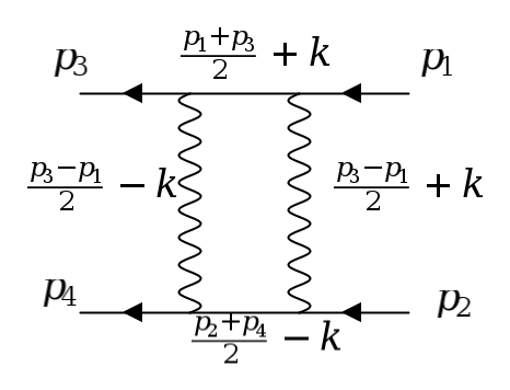
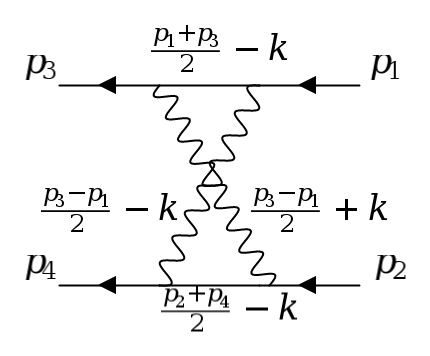
Figure 2: Two-photon exchange scattering amplitude.

In this section we apply the scattering amplitude approach to derive the two-photon part of the middle-energy contribution and the complete high-energy contribution. This part of the derivation will be performed in the Feynman gauge. In this section we will use the notations that $p_{1}$ and $p_{3}$ are the in and out momenta of the first electron, whereas $p_{2}$ and $p_{4}$ are the same for the second electron. We also define $P_{1}$ and $P_{2}$ as

$$\vec{P}_{1}=\frac{1}{2}(\vec{p}_{1}+\vec{p}_{3})\ \ \mbox{\rm and}\ \ \vec{P}_{2}=\frac{1}{2}(\vec{p}_{2}+\vec{p}_{4}).$$ (122)

The conservation of the total momentum and the kinetic energy leads to the following conditions,

$$\vec{p}_{1}+\vec{p}_{2} = \vec{p}_{3}+\vec{p}_{4}\,,$$

$$\frac{p_{1}^{2}}{2}+\frac{p_{2}^{2}}{2} = \frac{p_{3}^{2}}{2}+\frac{p_{4}^{2}}{2}\,.$$ (123)

The two-photon scattering amplitude is graphically represented in Fig. 2 and defined as

$$\mathcal{V} = -\frac{e^{4}}{2}\int\frac{d^{D}k}{(2\pi)^{D}\,i}\,\frac{1}{\big{(}k+\frac{p_{3}-p_{1}}{2}\big{)}^{2}}\,\frac{1}{\big{(}k-\frac{p_{3}-p_{1}}{2}\big{)}^{2}}$$ (124)

$$\times\bigg{\{}\overline{u}(p_{3})\,\gamma^{\mu}\,\frac{1}{\not{k}+\frac{1}{2}\,(\not{p}_{1}+\not{p}_{3})-m}\,\gamma^{\nu}\,u(p_{1})+\overline{u}(p_{3})\,\gamma^{\nu}\,\frac{1}{-\not{k}+\frac{1}{2}\,(\not{p}_{1}+\not{p}_{3})-m}\,\gamma^{\mu}\,u(p_{1})\bigg{\}}$$

$$\times\bigg{\{}\overline{u}(p_{4})\,\gamma^{\mu}\,\frac{1}{-\not{k}+\frac{1}{2}\,(\not{p}_{2}+\not{p}_{4})-m}\,\gamma^{\nu}\,u(p_{2})+\overline{u}(p_{4})\,\gamma^{\nu}\,\frac{1}{\not{k}+\frac{1}{2}\,(\not{p}_{2}+\not{p}_{4})-m}\,\gamma^{\mu}\,u(p_{2})\bigg{\}}\,,$$

where $u(p)$ are the free Dirac spinors. We aim to calculate the scattering amplitude in the middle-energy region (where $\omega\propto m\alpha,\,k\propto m\alpha$) and in the high-energy range (where $\omega\propto m,\,k\propto m$). External momenta $p_{i}$ are always of the order $m\alpha$. To separate out the spin-independent and spin-dependent parts, we make the following replacements, respectively,

$$u(p_{1})\,\overline{u}(p_{3}) \rightarrow\bigg{(}\frac{\not{p}_{1}+m}{\sqrt{2E_{p_{1}}(E_{p_{1}}+m)}}\bigg{)}\bigg{(}\frac{\gamma^{0}+I}{4}\bigg{)}\bigg{(}\frac{\not{p}_{3}+m}{\sqrt{2E_{p_{3}}(E_{p_{3}}+m)}}\bigg{)}$$ (125)

$$=\bigg{(}\frac{\not{p}_{1}+m}{2m}\bigg{)}\bigg{(}\frac{\gamma^{0}+I}{4}\bigg{)}\bigg{(}\frac{\not{p}_{3}+m}{2m}\bigg{)}\bigg{(}1-\frac{3}{8}\vec{p}_{1}{}^{2}-\frac{3}{8}\vec{p}_{3}{}^{2}\bigg{)}$$

and

$$u(p_{1})\,\overline{u}(p_{3}) \rightarrow\bigg{(}\frac{\not{p}_{1}+m}{\sqrt{2E_{p_{1}}(E_{p_{1}}+m)}}\bigg{)}\bigg{(}\frac{\gamma^{0}+I}{2}\bigg{)}\bigg{(}\frac{\sigma^{ij}}{4}\bigg{)}\bigg{(}\frac{\not{p}_{3}+m}{\sqrt{2E_{p_{3}}(E_{p_{3}}+m)}}\bigg{)}$$ (126)

$$=\bigg{(}\frac{\not{p}_{1}+m}{2m}\bigg{)}\bigg{(}\frac{\gamma^{0}+I}{2}\bigg{)}\bigg{(}\frac{\sigma^{ij}}{4}\bigg{)}\bigg{(}\frac{\not{p}_{3}+m}{2m}\bigg{)}\bigg{(}1-\frac{3}{8}\vec{p}_{1}{}^{2}-\frac{3}{8}\vec{p}_{3}{}^{2}\bigg{)}\,,$$

where $\sigma^{ij}=(i/2)\big{[}\gamma^{i},\gamma^{j}\big{]}$ and we used the fact that for the antisymmetric spin-dependent operator $\hat{Q}=Q^{ij}\sigma^{ij}$ the following identity holds

$$\hat{Q}=\frac{1}{4}\textrm{Tr}[\hat{Q}\cdot\sigma^{ij}]\,\sigma^{ij}\,.$$ (127)

For the spin-independent part of the scattering amplitude we get

$$\mathcal{V}_{nn} = -\frac{(4\pi\alpha)^{2}}{2}\int\frac{d^{D}k}{(2\pi)^{D}\,i}\,\frac{1}{\big{(}k+\frac{p_{3}-p_{1}}{2}\big{)}^{2}}\,\frac{1}{\big{(}k-\frac{p_{3}-p_{1}}{2}\big{)}^{2}}\,\bigg{(}1-\frac{3}{8}\vec{p}_{1}{}^{2}-\frac{3}{8}\vec{p}_{2}{}^{2}-\frac{3}{8}\vec{p}_{3}{}^{2}-\frac{3}{8}\vec{p}_{4}{}^{2}\bigg{)}$$ (128)

$$\times\,\textrm{Tr}\bigg{[}\bigg{(}\gamma^{\mu}\,\frac{1}{\not{k}+\frac{1}{2}\,(\not{p}_{1}+\not{p}_{3})-m}\,\gamma^{\nu}+\gamma^{\nu}\,\frac{1}{-\not{k}+\frac{1}{2}\,(\not{p}_{1}+\not{p}_{3})-m}\,\gamma^{\mu}\bigg{)}\bigg{(}\frac{\not{p}_{1}+m}{2m}\bigg{)}\bigg{(}\frac{\gamma^{0}+I}{4}\bigg{)}\bigg{(}\frac{\not{p}_{3}+m}{2m}\bigg{)}\bigg{]}$$

$$\times\,\textrm{Tr}\bigg{[}\bigg{(}\gamma^{\mu}\,\frac{1}{-\not{k}+\frac{1}{2}\,(\not{p}_{2}+\not{p}_{4})-m}\,\gamma^{\nu}+\gamma^{\nu}\,\frac{1}{\not{k}+\frac{1}{2}\,(\not{p}_{2}+\not{p}_{4})-m}\,\gamma^{\mu}\bigg{)}\bigg{(}\frac{\not{p}_{2}+m}{2m}\bigg{)}\bigg{(}\frac{\gamma^{0}+I}{4}\bigg{)}\bigg{(}\frac{\not{p}_{4}+m}{2m}\bigg{)}\bigg{]}\,.$$

The spin-dependent part of the scattering amplitude is

$$\mathcal{V}_{ss}=\mathcal{V}_{ss}^{ij,ab}\sigma_{1}^{ij}\sigma_{2}^{ab}\,,$$ (129)

where

$$\mathcal{V}_{ss}^{ij,ab} = \frac{(4\pi\alpha)^{2}}{2}\int\frac{d^{D}k}{(2\pi)^{D}\,i}\,\frac{1}{\big{(}k+\frac{p_{3}-p_{1}}{2}\big{)}^{2}}\,\frac{1}{\big{(}k-\frac{p_{3}-p_{1}}{2}\big{)}^{2}}\,\bigg{(}1-\frac{3}{8}\vec{p}_{1}{}^{2}-\frac{3}{8}\vec{p}_{2}{}^{2}-\frac{3}{8}\vec{p}_{3}{}^{2}-\frac{3}{8}\vec{p}_{4}{}^{2}\bigg{)}$$

$$\times\,\textrm{Tr}\bigg{[}\bigg{(}\gamma^{\mu}\,\frac{1}{\not{k}+\frac{1}{2}\,(\not{p}_{1}+\not{p}_{3})-m}\,\gamma^{\nu}+\gamma^{\nu}\,\frac{1}{-\not{k}+\frac{1}{2}\,(\not{p}_{1}+\not{p}_{3})-m}\,\gamma^{\mu}\bigg{)}\bigg{(}\frac{\not{p}_{1}+m}{2m}\bigg{)}\bigg{(}\frac{\gamma^{0}+I}{2}\bigg{)}\frac{1}{8}\big{[}\gamma^{i},\gamma^{j}\big{]}\bigg{(}\frac{\not{p}_{3}+m}{2m}\bigg{)}\bigg{]}$$

$$\times\,\textrm{Tr}\bigg{[}\bigg{(}\gamma^{\mu}\,\frac{1}{-\not{k}+\frac{1}{2}\,(\not{p}_{2}+\not{p}_{4})-m}\,\gamma^{\nu}+\gamma^{\nu}\,\frac{1}{\not{k}+\frac{1}{2}\,(\not{p}_{2}+\not{p}_{4})-m}\,\gamma^{\mu}\bigg{)}\bigg{(}\frac{\not{p}_{2}+m}{2m}\bigg{)}\bigg{(}\frac{\gamma^{0}+I}{2}\bigg{)}\frac{1}{8}\big{[}\gamma^{a},\gamma^{b}\big{]}\bigg{(}\frac{\not{p}_{4}+m}{2m}\bigg{)}\bigg{]}\,.$$

We now perform traces and then rescale the photon and fermion momenta for either middle-energy or high-energy contributions. Then we expand the expression in $\alpha$ and pick up the contribution of the order $\alpha^{7}$. After performing the trivial $\omega$ integration, the remaining integrals are handled using formulas from Appendix C. After the angular averaging using relations from Appendix B, we obtain the following result in the momentum representation for the middle-energy contribution,

$$H_{M} = \frac{\alpha^{2}}{m^{4}}\bigg{\{}\biggl{(}-\frac{7q^{2}}{36}-\frac{q^{2}}{24\epsilon}+\frac{q^{2}}{12}\ln q\biggr{)}\,\sigma_{1}\cdot\sigma_{2}+\frac{19}{30}(\vec{P}_{1}-\vec{P}_{2})^{2}-\frac{1}{3}\vec{P}_{1}\cdot\vec{P}_{2}-\frac{4}{5}q^{2}-\frac{7}{3}\frac{(\vec{P}_{1}\cdot\vec{q})(\vec{P}_{2}\cdot\vec{q})}{q^{2}}$$ (131)

$$+\biggl{(}-\frac{7}{15}(\vec{P}_{1}-\vec{P}_{2})^{2}-\frac{14}{3}\vec{P}_{1}\cdot\vec{P}_{2}-\frac{46}{15}q^{2}\biggr{)}\bigg{(}-\frac{1}{2\epsilon}+\ln q\bigg{)}\bigg{\}}\,.$$

This result agrees with the formula (120) obtained within the NRQED approach in the previous section, with the exception of terms proportional to $\bigl{(}(\vec{P}_{1}-\vec{P}_{2})\cdot\vec{q}\,\bigr{)}^{2}/q^{2}$. This is because $(\vec{P}_{1}-\vec{P}_{2})\cdot\vec{q}=\frac{1}{2}(p_{3}^{2}+p_{4}^{2}-p_{1}^{2}-p_{2}^{2})=0$ for the scattering amplitude due to the conservation of the kinetic energy. Therefore, the corresponding contribution cannot be derived from the two-photon amplitude. This contribution can be in principle obtained from the three-photon scattering amplitude, by transforming it into the three-photon exchange form by using the Schrödinger equation, as shown in the next section. However, the calculation of the middle-energy part from the three-photon exchange scattering amplitude was too complicated for us to be pursued, in contrast to the NRQED approach, where the corresponding derivation is relatively simple.

The result the high-energy contribution is

$$H_{H} = \frac{\alpha^{2}}{m^{4}}\bigg{\{}-\frac{56}{45}(\vec{P}_{1}-\vec{P}_{2})^{2}-\frac{2}{3}\vec{P}_{1}\cdot\vec{P}_{2}+\frac{13}{10}q^{2}+\frac{1}{\epsilon}\biggl{[}\frac{1}{6}(\vec{P}_{1}-\vec{P}_{2})^{2}-\vec{P}_{1}\cdot\vec{P}_{2}-q^{2}\biggr{]}$$ (132)

$$+\biggl{(}\frac{11}{54}(\vec{P}_{1}-\vec{P}_{2})^{2}+\frac{1}{2}\vec{P}_{1}\cdot\vec{P}_{2}+\frac{7}{36}q^{2}+\frac{11}{72\epsilon}q^{2}\biggr{)}\,\sigma_{1}\cdot\sigma_{2}\bigg{\}}\,,$$

and there is no three-photon high-energy part.

VI Total result in momentum space

The total result for $H_{\rm exch}^{(7)}$ is a sum of the low-energy, middle-energy and high-energy contributions, see Eq. (6). In order to obtain the total result, we perform a transformation of the two-photon term $\langle[(\vec{P}_{1}-\vec{P}_{2})\cdot\vec{q}]^{2}\,f(\vec{q})\rangle$, which is in coordinate representation

$$\biggl{\langle}\frac{1}{4}\bigl{[}p_{1}^{2}+p_{2}^{2}\,,\,\bigl{[}p_{1}^{2}+p_{2}^{2}\,,\,f(\vec{r})\bigr{]}\bigr{]}\biggr{\rangle}=-\biggl{\langle}\frac{1}{2}\bigl{[}V\,,\,\bigl{[}p_{1}^{2}+p_{2}^{2}\,,\,f(\vec{r})\bigr{]}\bigr{]}\biggr{\rangle}=-\bigl{\langle}\bigl{[}V\,,\,\vec{p}_{1}\bigr{]}\,\bigl{[}\vec{p}_{1}\,,\,f(\vec{r})\bigr{]}\bigr{\rangle}+(1\leftrightarrow 2)\,$$ (133)

and thus can be rewritten as a three-photon contribution. The two-body part of this contribution is further transformed using the integration formula with $\ln q$ in Eq. (205) from Appendix C. Finally, we obtain

$$H_{\rm exch}^{(7)} = \frac{\alpha^{2}}{m^{4}}\bigg{\{}\,\sigma_{1}\cdot\sigma_{2}\biggl{(}-\frac{7}{27}q^{2}+\frac{11}{54}(\vec{P}_{1}-\vec{P}_{2})^{2}+\frac{1}{2}\vec{P}_{1}\cdot\vec{P}_{2}-\frac{2}{9}q^{2}\ln[\alpha^{-2}]+\frac{2}{9}q^{2}\ln(2\lambda)+\frac{1}{12}q^{2}\ln q\biggr{)}$$ (134)

$$+\bigg{(}-\frac{527}{450}-\frac{4}{5}\ln[\alpha^{-2}]+\frac{4}{5}\ln(2\lambda)-\frac{7}{15}\ln q\bigg{)}(\vec{P}_{1}-\vec{P}_{2})^{2}$$

$$+\bigg{(}-\frac{151}{450}-\frac{16}{15}\ln[\alpha^{-2}]+\frac{16}{15}\ln(2\lambda)-\frac{46}{15}\ln q\bigg{)}q^{2}$$

$$+\bigg{(}-\frac{109}{45}-\frac{8}{3}\ln[\alpha^{-2}]+\frac{8}{3}\ln(2\lambda)-\frac{14}{3}\ln q\bigg{)}\vec{P}_{1}\cdot\vec{P}_{2}-\frac{31}{15}\frac{(\vec{P}_{1}\cdot\vec{q})(\vec{P}_{2}\cdot\vec{q})}{q^{2}}\bigg{\}}$$

$$+\frac{\pi\alpha^{3}}{m^{3}}\bigg{(}-\frac{161}{225}+\frac{8}{15}\ln[\alpha^{-2}]-\frac{8}{15}\ln(2\lambda)+\frac{4}{5}\ln 2+\frac{8}{15}\ln q\bigg{)}\,q$$

$$+\frac{\alpha^{3}}{m^{3}}\bigg{\{}\langle\phi|\bigg{[}p_{2}^{j},-\frac{Z}{r_{2}}\bigg{]}\bigg{(}\frac{26}{225}-\frac{8}{15}\ln[\alpha^{-2}]+\frac{8}{15}\ln(2\lambda)-\frac{8}{5}\ln 2-\frac{8}{15}\ln q\bigg{)}\frac{q^{j}}{q^{2}}$$

$$+\bigg{[}\bigg{[}p_{2}^{i},-\frac{Z}{r_{2}}\bigg{]},p_{2}^{j}\bigg{]}\bigg{[}\delta^{ij}\bigg{(}-\frac{436}{225}-\frac{32}{15}\ln[\alpha^{-2}]+\frac{32}{15}\ln(2\lambda)-\frac{32}{15}\ln q\bigg{)}$$

$$+\frac{q^{i}q^{j}}{q^{2}}\bigg{(}-\frac{236}{225}+\frac{8}{15}\ln[\alpha^{-2}]-\frac{8}{15}\ln(2\lambda)+\frac{8}{15}\ln q\bigg{)}\bigg{]}\frac{1}{q^{2}}|\phi\rangle+(1\leftrightarrow 2)\bigg{\}}\,.$$

In order to make the transformation of the above expression into coordinate space more accessible, we need to express the momenta $\vec{P}_{1}$ and $\vec{P}_{2}$ in terms $\vec{P}$, $\vec{p}$, and $\vec{q}$ defined as

$$\vec{P}= \ \vec{p}_{1}+\vec{p}_{2}\,,\ \ \vec{p}=\frac{1}{2}\big{(}\vec{p}_{1}-\vec{p}_{2}\big{)}\,,\ \ \mbox{\rm and}\ \ \vec{q}=\vec{p}_{1}{}^{\prime}-\vec{p}_{1}\,.$$ (135)

We thus have

$$\big{(}\vec{P}_{1}-\vec{P}_{2}\big{)}^{2} = q^{2}+4\,\vec{p}\cdot\vec{p}\,{}^{\prime}\,,$$ (136)

$$\vec{P}_{1}\cdot\vec{P}_{2} = \frac{1}{4}\bigg{(}P^{2}-q^{2}-4\,\vec{p}\cdot\vec{p}\,{}^{\prime}\bigg{)}\,,$$ (137)

$$\frac{(\vec{P}_{1}\cdot\vec{q})(\vec{P}_{2}\cdot\vec{q})}{q^{2}} = \bigg{(}\frac{1}{4}P^{i}P^{j}-p^{i}p^{\prime j}\bigg{)}\frac{q^{i}q^{j}-\frac{\delta^{ij}}{3}q^{2}}{q^{2}}-\frac{1}{4}q^{2}+\frac{1}{12}P^{2}-\frac{1}{3}\,\vec{p}\cdot\vec{p}\,{}^{\prime}\,.$$ (138)

We also use $\sigma_{1}\cdot\sigma_{2}=2\,\vec{\sigma}_{1}\cdot\vec{\sigma}_{2}$, which is valid in $d=3$, and neglect operators $P^{2}\,\delta^{3}(r)$ and $p^{2}\,\delta^{3}(r)$, which vanish for triplet states. Furthermore, for triplet states we can assume $\vec{\sigma}_{1}\cdot\vec{\sigma}_{2}=1$. The total result for $H_{\rm exch}^{(7)}$ in momentum space after these transformations becomes

$$H^{(7)}_{\rm exch} = \frac{\alpha^{2}}{m^{4}}\bigg{\{}\frac{14}{5}\vec{p}\cdot\vec{p}\,{}^{\prime}\,\ln q-\frac{7}{6}\,P^{2}\ln q-\frac{31}{60}\big{(}P^{i}P^{j}-4p^{i}p^{\prime j}\big{)}\,\biggl{(}q^{i}q^{j}-\frac{\delta^{ij}}{3}q^{2}\biggr{)}\frac{1}{q^{2}}$$ (139)

$$+\bigg{(}-\frac{739}{2700}-\frac{62}{45}\ln[\alpha^{-2}]+\frac{62}{45}\ln(2\lambda)-\frac{11}{5}\ln q\bigg{)}q^{2}\bigg{\}}$$

$$+\frac{\pi\alpha^{3}}{m^{3}}\bigg{(}-\frac{161}{225}+\frac{8}{15}\ln[\alpha^{-2}]-\frac{8}{15}\ln(2\lambda)+\frac{4}{5}\ln 2+\frac{8}{15}\ln q\bigg{)}\,q$$

$$+\frac{\alpha^{3}}{m^{3}}\bigg{\{}\bigg{[}p_{2}^{j},-\frac{Z}{r_{2}}\bigg{]}\bigg{(}\frac{26}{225}-\frac{8}{15}\ln[\alpha^{-2}]+\frac{8}{15}\ln(2\lambda)-\frac{8}{5}\ln 2-\frac{8}{15}\ln q\bigg{)}\frac{q^{j}}{q^{2}}$$

$$+\bigg{[}\bigg{[}p_{2}^{i},-\frac{Z}{r_{2}}\bigg{]},p_{2}^{j}\bigg{]}\bigg{[}\delta^{ij}\bigg{(}-\frac{436}{225}-\frac{32}{15}\ln[\alpha^{-2}]+\frac{32}{15}\ln(2\lambda)-\frac{32}{15}\ln q\bigg{)}$$

$$+\frac{q^{i}q^{j}}{q^{2}}\bigg{(}-\frac{236}{225}+\frac{8}{15}\ln[\alpha^{-2}]-\frac{8}{15}\ln(2\lambda)+\frac{8}{15}\ln q\bigg{)}\bigg{]}\frac{1}{q^{2}}+(1\leftrightarrow 2)\bigg{\}}\,.$$

In spite of quite lengthy calculations, this result is relatively simple. We expect that it will be further simplified after adding the radiative contribution.

VII Total result in coordinate space

We now transform the obtained formulas for $H_{\rm exch}^{(7)}$ into the coordinate representation in atomic units, which is needed for the numerical evaluation of the matrix element with the nonrelativistic wave function. All momenta are rescaled $p\rightarrow\alpha\,p$, so $\ln q\rightarrow\ln\alpha+\ln q$, and the overall factor $\alpha^{7}$ is pulled out of $H^{(7)}_{\rm exch}$. In order to perform the Fourier transform, we start with the master integral formula in $d$ dimensions,

$$\int\frac{d^{d}q}{(2\pi)^{d}}\,q^{m}\,e^{i\vec{q}\cdot\vec{r}} = \frac{\pi^{-d/2}2^{m}\left(r^{2}\right)^{\frac{1}{2}(-d-m)}\Gamma\left(\frac{d+m}{2}\right)}{\Gamma\left(-\frac{m}{2}\right)}\,.$$ (140)

From the above formula, we derive the following results for the $d=3$ Fourier transforms of various operators,

$$\int\frac{d^{3}q}{(2\pi)^{3}}\,e^{i\vec{q}\cdot\vec{r}}\,\frac{4\pi}{q^{2}}= \,\frac{1}{r}\,,$$ (141)

$$\int\frac{d^{3}q}{(2\pi)^{3}}\,e^{i\vec{q}\cdot\vec{r}}\,\frac{4\pi}{q^{2}}\,\ln q= \,-\frac{\gamma+\ln r}{r}\,,$$ (142)

$$\int\frac{d^{3}q}{(2\pi)^{3}}\,e^{i\vec{q}\cdot\vec{r}}\,4\pi\frac{q^{i}}{q^{2}}= \,i\frac{r^{i}}{r^{3}}\,,$$ (143)

$$\int\frac{d^{3}q}{(2\pi)^{3}}\,e^{i\vec{q}\cdot\vec{r}}\,4\pi\frac{q^{i}}{q^{2}}\,\ln q= \,i\frac{r^{i}}{r^{3}}(1-\gamma-\ln r)\,,$$ (144)

$$\int\frac{d^{3}q}{(2\pi)^{3}}\,e^{i\vec{q}\cdot\vec{r}}\,4\pi\frac{q^{i}q^{j}-\frac{\delta^{ij}}{3}q^{2}}{q^{2}}= \,\frac{\delta^{ij}r^{2}-3r^{i}r^{j}}{r^{5}}\,,$$ (145)

$$\int\frac{d^{3}q}{(2\pi)^{3}}\,e^{i\vec{q}\cdot\vec{r}}\,4\pi\,\frac{q^{i}q^{j}}{q^{4}}= \,\frac{1}{2r^{3}}\big{(}\delta^{ij}r^{2}-r^{i}r^{j}\big{)}\,,$$ (146)

$$\int\frac{d^{3}q}{(2\pi)^{3}}\,e^{i\vec{q}\cdot\vec{r}}\,4\pi\,\frac{q^{i}q^{j}}{q^{4}}\,\ln q= \,-\nabla^{i}\nabla^{j}\bigg{[}\frac{r}{4}\big{(}-3+2\gamma+2\ln r\big{)}\bigg{]}$$

$$= \,\frac{1}{4}\bigg{[}\frac{\delta^{ij}r^{2}-3r^{i}r^{j}}{r^{3}}-\frac{\big{(}\delta^{ij}r^{2}-r^{i}r^{j}\big{)}}{r^{3}}\big{(}2\gamma+2\ln r\big{)}\bigg{]}\,.$$ (147)

The right-hand sides of the above formulas for the Fourier transforms are well-defined functions. However, there are some operators in $H^{(7)}_{\rm exch}$ that require more careful treatment. We now take into account that the matrix element of $H^{(7)}_{\rm exch}$ is calculated with the antisymmetric wave function, which satisfies the condition $\phi(\vec{r}_{1},\vec{r}_{2})=-\phi(\vec{r}_{2},\vec{r}_{1})$. Therefore, the wave function behaves as $\phi(\vec{r})\sim\vec{r}\cdot(\vec{r}_{1}+\vec{r}_{2})$ for small $|\vec{r}|$. Under this condition, matrix elements of all operators in $H^{(7)}_{\rm exch}$ in momentum representation are finite and well defined. Their transformation in the coordinate space, however, may require special definitions.

We now define the coordinate-space representation of all singular operators in $H^{(7)}_{\rm exch}$. We start with the well-known operator $(1/r^{3})_{\varepsilon}$, which is defined by the integral with an arbitrary smooth function $f(\vec{r})$ as follows

$$\int d^{3}r\,f(\vec{r})\,\Bigl{(}\frac{1}{r^{3}}\Bigr{)}_{\varepsilon}=\lim_{\varepsilon\rightarrow 0}\int d^{3}r\,f(\vec{r})\,\bigg{[}\frac{1}{r^{3}}\theta(r-\varepsilon)+4\pi\delta^{3}(r)(\gamma+\ln\varepsilon)\bigg{]}\,.$$ (148)

The Dirac delta function in the above definition appears because the $(1/r^{3})_{\varepsilon}$ operator is assumed to be sandwiched between two momenta operators, $\vec{p}\,(1/r^{3})_{\varepsilon}\,\vec{p}$. The Fourier transform of $(1/r^{3})_{\varepsilon}$ is evaluated as

$$\int d^{3}r\,e^{i\vec{q}\cdot\vec{r}}\,\Bigl{(}\frac{1}{r^{3}}\Bigr{)}_{\varepsilon} = \lim_{\varepsilon\rightarrow 0}\int d^{3}r\,e^{i\vec{q}\cdot\vec{r}}\bigg{[}\frac{1}{r^{3}}\theta(r-\varepsilon)+4\pi\delta^{3}(r)(\gamma+\ln\varepsilon)\bigg{]}$$ (149)

$$= \lim_{\varepsilon\rightarrow 0}2\pi\int_{-1}^{1}dx\int_{\varepsilon}^{\infty}\frac{dr}{r}\,e^{iqrx}+4\pi(\gamma+\ln\varepsilon)=4\pi(1-\ln q)\,.$$

The operator $(1/r^{4})_{\varepsilon}$ is defined by

$$\int d^{3}r\,f(\vec{r})\,\Bigl{(}\frac{1}{r^{4}}\Bigr{)}_{\varepsilon}=\lim_{\varepsilon\rightarrow 0}\int d^{3}r\,f(\vec{r})\,\bigg{[}\frac{1}{r^{4}}\theta(r-\varepsilon)-4\pi\delta^{3}(r)\,\frac{1}{\varepsilon}\bigg{]}\,.$$ (150)

Its Fourier transform is

$$\int d^{3}r\,e^{i\vec{q}\cdot\vec{r}}\,\Bigl{(}\frac{1}{r^{4}}\Bigr{)}_{\varepsilon} = \lim_{\varepsilon\rightarrow 0}\int d^{3}r\,e^{i\vec{q}\cdot\vec{r}}\bigg{[}\frac{1}{r^{4}}\theta(r-\varepsilon)-4\pi\delta^{3}(r)\,\frac{1}{\varepsilon}\bigg{]}$$ (151)

$$= \lim_{\varepsilon\rightarrow 0}2\pi\int_{-1}^{1}dx\int_{\varepsilon}^{\infty}\frac{dr}{r^{2}}\,e^{iqrx}-\frac{4\pi}{\varepsilon}=-\pi^{2}\,q\,.$$

Similarly, $(\ln r/r^{4})_{\varepsilon}$ is defined by

$$\int d^{3}r\,f(\vec{r})\,\Bigl{(}\frac{\ln r}{r^{4}}\Bigr{)}_{\varepsilon}=\lim_{\varepsilon\rightarrow 0}\int d^{3}r\,f(\vec{r})\,\bigg{[}\frac{\ln r}{r^{4}}\theta(r-\varepsilon)-4\pi\delta^{3}(r)\,\frac{1+\ln\varepsilon}{\varepsilon}\bigg{]}\,.$$ (152)

Its Fourier transform is

$$\int d^{3}r\,e^{i\vec{q}\cdot\vec{r}}\,\Bigl{(}\frac{\ln r}{r^{4}}\Bigr{)}_{\varepsilon} = \lim_{\varepsilon\rightarrow 0}\int d^{3}r\,e^{i\vec{q}\cdot\vec{r}}\bigg{[}\frac{\ln r}{r^{4}}\,\theta(r-\varepsilon)-4\pi\delta^{3}(r)\,\frac{1+\ln\varepsilon}{\varepsilon}\bigg{]}$$ (153)

$$= \lim_{\varepsilon\rightarrow 0}2\pi\int_{-1}^{1}dx\int_{\varepsilon}^{\infty}\frac{dr}{r^{2}}\ln r\,e^{iqrx}-4\pi\,\frac{1+\ln\varepsilon}{\varepsilon}=\pi^{2}\bigg{(}-\frac{3}{2}+\gamma+\ln q\bigg{)}\,q\,.$$

The operator $(1/r^{5})_{\varepsilon}$ is defined by

$$\int d^{3}r\,f(\vec{r})\,\Bigl{(}\frac{1}{r^{5}}\Bigr{)}_{\varepsilon}=\lim_{\varepsilon\rightarrow 0}\int d^{3}r\,f(\vec{r})\,\bigg{[}\frac{1}{r^{5}}\,\theta(r-\varepsilon)-2\pi\delta^{3}(r)\,\frac{1}{\varepsilon^{2}}+\frac{2}{3}\pi\nabla^{2}\delta^{3}(r)\,(\gamma+\ln\varepsilon)\bigg{]}\,,$$ (154)

with the corresponding Fourier transform evaluated as

$$\int d^{3}r\,e^{i\vec{q}\cdot\vec{r}}\,\Bigl{(}\frac{1}{r^{5}}\Bigr{)}_{\varepsilon} = \lim_{\varepsilon\rightarrow 0}\int d^{3}r\,e^{i\vec{q}\cdot\vec{r}}\bigg{[}\frac{1}{r^{5}}\,\theta(r-\varepsilon)-2\pi\delta^{3}(r)\,\frac{1}{\varepsilon^{2}}+\frac{2}{3}\pi\nabla^{2}\delta^{3}(r)\,(\gamma+\ln\varepsilon)\bigg{]}$$ (155)

$$= 2\pi\int_{-1}^{1}dx\int_{\varepsilon}^{\infty}\frac{dr}{r^{3}}\,e^{iqrx}-2\pi\,\frac{1}{\varepsilon^{2}}-\frac{2}{3}\pi\big{(}\gamma+\ln\varepsilon)\,q^{2}=\pi\bigg{(}-\frac{11}{9}+\frac{2}{3}\ln q\bigg{)}\,q^{2}\,.$$

Using the above formulas, the final result for $H^{(7)}_{\rm exch}$ in the coordinate representations is obtained as

$$H^{(7)}_{\rm exch} = \bigg{(}\frac{15\,409}{1350}-\frac{124}{45}\ln(2\lambda)+\frac{76}{45}\ln\alpha\bigg{)}\,\vec{p}\,\delta^{(3)}(r)\,\vec{p}-\frac{33}{10\pi\,r^{5}}$$ (156)

$$-\frac{7}{10\pi}\,\vec{p}\,\frac{1}{r^{3}}\,\vec{p}+\frac{7}{24\pi}P^{2}\,\frac{1}{r^{3}}+\frac{31}{60\pi}\,p^{i}\,\frac{\delta^{ij}r^{2}-3r^{i}r^{j}}{r^{5}}\,p^{j}-\frac{31}{240\pi}\,P^{i}P^{j}\,\frac{\delta^{ij}r^{2}-3r^{i}r^{j}}{r^{5}}$$

$$+\frac{8}{15\pi\,r^{4}}\bigg{(}-\frac{19}{120}-\frac{3}{2}\ln 2+\ln(2\lambda)+\ln\alpha+\gamma+\ln r\bigg{)}$$

$$+\bigg{\{}-\frac{2\,Z}{15\pi}\frac{\vec{r}_{1}\cdot\vec{r}}{r_{1}^{3}r^{3}}\bigg{(}-\frac{47}{60}-3\ln 2+\ln(2\lambda)+\ln\alpha+\gamma+\ln r\bigg{)}$$

$$+\frac{Z}{15\pi}\frac{\big{(}\delta^{ij}r_{1}^{2}-3r_{1}^{i}r_{1}^{j}\big{)}r^{i}r^{j}}{r_{1}^{5}r^{3}}\bigg{(}\frac{7}{15}+\ln(2\lambda)+\ln\alpha+\gamma+\ln r\bigg{)}$$

$$+\frac{88}{45}Z\,\delta^{(3)}(r_{1})\frac{1}{r}\bigg{(}-\frac{193}{165}+\ln(2\lambda)+\ln\alpha+\gamma+\ln r\bigg{)}+(1\leftrightarrow 2)\bigg{\}}\,,$$

where $\vec{p}=(\vec{p}_{1}-\vec{p}_{2})/2$, $\vec{P}=\vec{p}_{1}+\vec{p}_{2}$. Additional terms with $\ln\alpha$ are obtained from the transformation into atomic units $\ln q\rightarrow\ln q+\ln\alpha$. We stress that this form of $H^{(7)}_{\rm exch}$ is valid only for antisymmetric states. Eq. (156) is the main result of this work. Despite the very complicated derivation, the final result for $H^{(7)}_{\rm exch}$ has a very simple form consisting of just a few operators.

VIII Summary

In this work we calculated the QED effects of the order $\alpha^{7}m$ to the Lamb shift, which originate from the virtual photon exchange between the electrons and the nucleus and are represented by two- and three-photon exchange diagrams. The central problem was the derivation of the effective Hamiltonian $H^{(7)}_{\rm exch}$ in coordinate space. The corresponding result valid for the antisymmetric (triplet) states of two-electron atoms is given by Eq. (156). The obtained expression is free from any singularities (provided that the expectation value is calculated with wave functions of antisymmetric states). The final expression was obtained after delicate cancellations of numerous divergences present in individual operators in momentum space. It is finite but still depends on the photon-momentum cutoff parameter $\lambda$. This dependence will disappear when $H^{(7)}_{\rm exch}$ is combined together with the radiative and low-energy contributions in Eq. (5).

The numerical evaluation of the expectation value of $H^{(7)}_{\rm exch}$ would be straightforward, because many operators have already been encountered in our previous studies patkos:16:triplet ; patkos:17:singlet and other operators are of a similar complexity. However, the numerical value of $\langle H^{(7)}_{\rm exch}\rangle$ would not be useful for a comparison with experimental results, because of dependence on the cutoff parameter $\lambda$. For this reason we have postponed the numerical evaluation until the radiative corrections are calculated, which we plan to accomplish in the forthcoming investigation.

Calculations of the remaining part, namely the radiative $\alpha^{7}m$ effects, will be greatly simplified by the fact that these effects are known for the hydrogenic atoms. Specifically, the one-loop $\alpha^{7}\,m$ correction (the so-called $A_{60}$ coefficient) was derived in Ref. pachucki:93 . The corresponding two-loop contribution (the so-called $B_{50}$ coefficient) was calculated in Refs. pachucki:94 ; eides:95:pra , whereas the three-loop contribution $C_{40}$ was completed in Ref. melnikov:00 . The two- and three-loop corrections are proportional to the electron charge density on the nucleus, so only the one-loop radiative contribution needs to be re-derived for the helium atom.

In the present work we performed our derivation for the triplet states of helium only. The restriction to these states was made because their wave function is antisymmetric with respect to exchange of spatial electron coordinates and vanishes at $\vec{r}_{1}=\vec{r}_{2}$, which greatly simplifies the derivation. An extension of the present derivation to the singlet states of helium might be possible but would involve a calculation of four-photon exchange diagrams, the feasibility of which is not clear at present. Finally, the derivation of this work can be extended to many other bound systems, particularly to positronium, where a calculation of the $\alpha^{7}\,m$ QED effects has been required for a long time but has not yet been accomplished.

Appendix A Foldy-Wouthuysen transformation

The discussion in this section is based on our previous work fw . The Foldy-Wouthuysen (FW) transformation is a widely used method to derive the nonrelativistic expansion of the Dirac Hamiltonian in an external electromagnetic field,

$$H=\vec{\alpha}\cdot\vec{\pi}+\beta\,m+e\,A^{0}\,,$$ (157)

where $\vec{\pi}=\vec{p}-e\,\vec{A}$. The idea of the FW transformation is to apply a unitary transformation to the Dirac Hamiltonian that decouples the upper and lower components of the Dirac wave function up to a specified order in the $1/m$ expansion. The result is the FW Hamiltonian $H_{\rm FW}$ defined as

$$H_{\rm FW}=e^{i\,S}\,(H-i\,\partial_{t})\,e^{-i\,S}\,,$$ (158)

where $S$ is the operator that needs to be determined. In the this work we calculate the FW Hamiltonian up to terms that contribute to the order $\alpha^{7}\,m$ to the energy.

The choice of the unitary transformation operator $S$, and therefore the resulting FW Hamiltonian, is not unique. We use an approach that is somewhat different from the one described in standard textbooks. Specifically, we use the single operator $S$ defined as

$$S = -\frac{i}{2\,m}\,\Big{[}\beta\,\vec{\alpha}\cdot\vec{\pi}-\frac{1}{3\,m^{2}}\,\beta\,(\vec{\alpha}\cdot\vec{\pi})^{3}+\frac{i\,e}{2\,m}\,\vec{\alpha}\cdot\vec{E}-\frac{\beta\,e}{4\,m^{2}}\,\vec{\alpha}\cdot\dot{\vec{E}}+Y\Big{]}\,,$$ (159)

where $Y$ is some odd operator $\{\beta,Y\}=0$ which satisfies the condition $[Y,e\,A^{0}-i\,\partial_{t}]\approx[Y,(\vec{\alpha}\cdot\vec{\pi})^{3}]\approx 0$. We will fix the explicit form of $Y$ in the very end; this choice will allow us to cancel the unwanted higher-order odd terms. The FW Hamiltonian is expanded in a power series in $S$

$$H_{\rm FW}=\sum_{j=0}^{6}{\cal H}^{(j)}+\ldots\,,$$ (160)

where

$${\cal H}^{(0)}=H\,,\ \ \ {\cal H}^{(1)}=[i\,S\,,{\cal H}^{(0)}-i\,\partial_{t}]\,,\ \ \ {\cal H}^{(j)}=\frac{1}{j}\,[i\,S\,,{\cal H}^{(j-1)}]\;{\mbox{\rm for $j>1$}},$$ (161)

and terms with $j>6$ are neglected. The calculations of subsequent commutators is straightforward but rather tedious. For the reader’s convenience we present separate results for each $H^{(j)}$,

$${\cal H}^{(1)} = \frac{\beta}{m}\,(\vec{\alpha}\cdot\vec{\pi})^{2}-\frac{\beta}{3\,m^{3}}\,(\vec{\alpha}\cdot\vec{\pi})^{4}-\frac{i\,e}{4\,m^{2}}[\vec{\alpha}\cdot\vec{\pi},\vec{\alpha}\cdot\vec{E}]-\frac{e\,\beta}{8\,m^{3}}\{\vec{\alpha}\cdot\vec{\pi}\,,\,\vec{\alpha}\cdot\dot{\vec{E}}\}+\frac{1}{2\,m}[Y,\vec{\alpha}\cdot\vec{\pi}]$$ (162)

$$-\vec{\alpha}\cdot\vec{\pi}+\frac{1}{3\,m^{2}}\,(\vec{\alpha}\cdot\vec{\pi})^{3}-\beta\,Y-\frac{\beta}{6\,m^{3}}[(\vec{\alpha}\cdot\vec{\pi})^{3},e\,A^{0}-i\,\partial_{t}]-\frac{i\,\beta\,e}{8\,m^{2}}\,\vec{\alpha}\cdot\ddot{\vec{E}}\,,$$

$${\cal H}^{(2)} = -\frac{\beta}{2\,m}\,(\vec{\alpha}\cdot\vec{\pi})^{2}+\frac{\beta}{3\,m^{3}}\,(\vec{\alpha}\cdot\vec{\pi})^{4}-\frac{\beta}{18\,m^{5}}\,(\vec{\alpha}\cdot\vec{\pi})^{6}+\frac{i\,e}{8\,m^{2}}\,[\vec{\alpha}\cdot\vec{\pi},\vec{\alpha}\cdot\vec{E}]$$ (163)

$$-\frac{1}{2\,m}\,[Y,\vec{\alpha}\cdot\vec{\pi}]-\frac{i\,e}{24\,m^{4}}\,[(\vec{\alpha}\cdot\vec{\pi})^{3},\vec{\alpha}\cdot\vec{E}]+\frac{i\,e}{32\,m^{3}}\,[\vec{\alpha}\cdot\vec{\pi}\,,\,\vec{\alpha}\cdot\ddot{\vec{E}}]$$

$$+\frac{1}{24\,m^{4}}[\vec{\alpha}\cdot\vec{\pi},[(\vec{\alpha}\cdot\vec{\pi})^{3},e\,A^{0}-i\,\partial_{t}]]+\frac{e\,\beta}{16\,m^{3}}\,\bigl{\{}\vec{\alpha}\cdot\vec{\pi}\,,\,\vec{\alpha}\cdot\dot{\vec{E}}\bigr{\}}$$

$$-\frac{1}{2\,m^{2}}\,(\vec{\alpha}\cdot\vec{\pi})^{3}+\frac{1}{3\,m^{4}}\,(\vec{\alpha}\cdot\vec{\pi})^{5}-\frac{i\,\beta\,e}{16\,m^{3}}\,[\vec{\alpha}\cdot\vec{\pi},[\vec{\alpha}\cdot\vec{\pi},\vec{\alpha}\cdot\vec{E}]]$$

$$-\frac{i\,\beta\,e}{8\,m^{3}}\,\bigl{(}(\vec{\alpha}\cdot\vec{\pi})^{2}\,\vec{\alpha}\cdot\vec{E}+\vec{\alpha}\cdot\vec{E}\,(\vec{\alpha}\cdot\vec{\pi})^{2}\bigr{)}\,,$$

$${\cal H}^{(3)} = -\frac{\beta}{6\,m^{3}}\,(\vec{\alpha}\cdot\vec{\pi})^{4}+\frac{\beta}{6\,m^{5}}\,(\vec{\alpha}\cdot\vec{\pi})^{6}+\frac{i\,e}{96\,m^{4}}\,[\vec{\alpha}\cdot\vec{\pi},[\vec{\alpha}\cdot\vec{\pi},[\vec{\alpha}\cdot\vec{\pi},\vec{\alpha}\cdot\vec{E}]]]$$ (164)

$$+\frac{i\,e}{48\,m^{4}}\,[\vec{\alpha}\cdot\vec{\pi},(\vec{\alpha}\cdot\vec{\pi})^{2}\,\vec{\alpha}\cdot\vec{E}+\vec{\alpha}\cdot\vec{E}\,(\vec{\alpha}\cdot\vec{\pi})^{2}]+\frac{i\,e}{24\,m^{4}}\,[(\vec{\alpha}\cdot\vec{\pi})^{3},\vec{\alpha}\cdot\vec{E}]$$

$$+\frac{1}{6\,m^{2}}\,(\vec{\alpha}\cdot\vec{\pi})^{3}-\frac{1}{6\,m^{4}}\,(\vec{\alpha}\cdot\vec{\pi})^{5}+\frac{i\,\beta\,e}{48\,m^{3}}\,[\vec{\alpha}\cdot\vec{\pi},[\vec{\alpha}\cdot\vec{\pi},\vec{\alpha}\cdot\vec{E}]]$$

$$+\frac{i\,\beta\,e}{24\,m^{3}}\,\bigl{(}(\vec{\alpha}\cdot\vec{\pi})^{3}\,\vec{\alpha}\cdot\vec{E}+\vec{\alpha}\cdot\vec{E}\,(\vec{\alpha}\cdot\vec{\pi})^{3}\bigr{)}\,,$$

$${\cal H}^{(4)} = \frac{\beta}{24\,m^{3}}\,(\vec{\alpha}\cdot\vec{\pi})^{4}-\frac{\beta}{18\,m^{5}}\,(\vec{\alpha}\cdot\vec{\pi})^{6}-\frac{i\,e}{384}\,[\vec{\alpha}\cdot\vec{\pi},[\vec{\alpha}\cdot\vec{\pi},[\vec{\alpha}\cdot\vec{\pi},\vec{\alpha}\cdot\vec{E}]]]$$ (165)

$$-\frac{i\,e}{192\,m^{4}}\,[\vec{\alpha}\cdot\vec{\pi},(\vec{\alpha}\cdot\vec{\pi})^{2}\,\vec{\alpha}\cdot\vec{E}+\vec{\alpha}\cdot\vec{E}\,(\vec{\alpha}\cdot\vec{\pi})^{2}]-\frac{i\,e}{96\,m^{4}}\,[(\vec{\alpha}\cdot\vec{\pi})^{3},\vec{\alpha}\cdot\vec{E}]$$

$$+\frac{1}{24\,m^{4}}\,(\vec{\alpha}\cdot\vec{\pi})^{5}\,,$$

$${\cal H}^{(5)} = -\frac{1}{120\,m^{4}}\,(\vec{\alpha}\cdot\vec{\pi})^{5}+\frac{\beta}{120\,m^{5}}\,(\vec{\alpha}\cdot\vec{\pi})^{6}\,,$$ (166)

$${\cal H}^{(6)} = -\frac{\beta}{720\,m^{5}}\,(\vec{\alpha}\cdot\vec{\pi})^{6}\,.$$ (167)

At this stage the operator $H_{\rm FW}$ still depends on $Y$. Following the idea of the FW transformation, $Y$ is now chosen to cancel all the higher order odd terms from $H_{\rm FW}$,

$$Y = \frac{\beta}{5\,m^{4}}\,(\vec{\alpha}\cdot\vec{\pi})^{5}+\frac{i\,e}{24\,m^{3}}\,[\vec{\alpha}\cdot\vec{\pi},[\vec{\alpha}\cdot\vec{\pi},\vec{\alpha}\cdot\vec{E}]]-\frac{i\,e}{3\,m^{3}}\,\Big{(}(\vec{\alpha}\cdot\vec{\pi})^{2}\,\vec{\alpha}\cdot\vec{E}+\vec{\alpha}\cdot\vec{E}\,(\vec{\alpha}\cdot\vec{\pi})^{2}\Big{)}.$$ (168)

It can be seen that $Y$ fulfills the condition that commutators $[Y,e\,A^{0}-i\,\partial_{t}]$ and $[Y,(\vec{\alpha}\cdot\vec{\pi})^{3}]$ are of higher orders and thus can be neglected. The resulting FW Hamiltonian is

$$H_{\rm FW} = e\,A^{0}+\frac{(\vec{\sigma}\cdot\vec{\pi})^{2}}{2\,m}-\frac{(\vec{\sigma}\cdot\vec{\pi})^{4}}{8\,m^{3}}+\frac{(\vec{\sigma}\cdot\vec{\pi})^{6}}{16\,m^{5}}-\frac{i\,e}{8\,m^{2}}\,[\vec{\sigma}\cdot\vec{\pi},\vec{\sigma}\cdot\vec{E}]-\frac{e}{16\,m^{3}}\,\bigl{\{}\vec{\sigma}\cdot\vec{\pi}\,,\,\vec{\sigma}\cdot\dot{\vec{E}}\bigr{\}}+\frac{i\,e}{32\,m^{3}}\,[\vec{\sigma}\cdot\vec{\pi}\,,\,\vec{\sigma}\cdot\ddot{\vec{E}}]$$ (169)

$$-\frac{i\,e}{128\,m^{4}}\,[\vec{\sigma}\cdot\vec{\pi},[\vec{\sigma}\cdot\vec{\pi},[\vec{\sigma}\cdot\vec{\pi},\vec{\sigma}\cdot{\vec{E}}]]]+\frac{i\,e}{16\,m^{4}}\,\Bigl{(}(\vec{\sigma}\cdot\vec{\pi})^{2}\,[\vec{\sigma}\cdot\vec{\pi},\vec{\sigma}\cdot\vec{E}]+[\vec{\sigma}\cdot\vec{\pi},\vec{\sigma}\cdot\vec{E}]\,(\vec{\sigma}\cdot\vec{\pi})^{2}\Bigr{)},$$

where we used the following commutator identity to simplify the expression,

$$[(\vec{\sigma}\cdot\vec{\pi})^{3},\vec{\sigma}\cdot\vec{E}] = -\frac{1}{2}\,[\vec{\sigma}\cdot\vec{\pi},[\vec{\sigma}\cdot\vec{\pi},[\vec{\sigma}\cdot\vec{\pi},\vec{\sigma}\cdot{\vec{E}}]]]+\frac{3}{2}\,\Bigl{(}(\vec{\sigma}\cdot\vec{\pi})^{2}\,[\vec{\sigma}\cdot\vec{\pi},\vec{\sigma}\cdot\vec{E}]+[\vec{\sigma}\cdot\vec{\pi},\vec{\sigma}\cdot\vec{E}]\,(\vec{\sigma}\cdot\vec{\pi})^{2}\Bigr{)}\,.$$ (170)

Due to non-uniqueness in the operator $S$, the FW Hamiltonian $H_{\rm FW}$ given by Eq. (169) differs from the one that can be obtained by the standard textbook approach (relying on the subsequent use of the FW transformations) by the transformation $S$ with some additional even operator. However, all variants of the FW Hamiltonian have to be equivalent at the level of matrix elements between the states that satisfy the Schrödinger equation.

For the purpose of calculation of the $\alpha^{7}\,m$ contribution we use the following FW Hamiltonian

$$H_{\rm FW} = eA^{0}+\frac{(\vec{\sigma}\cdot\vec{\pi})^{2}}{2m}-\frac{(\vec{\sigma}\cdot\vec{\pi})^{4}}{8m^{3}}+\frac{(\vec{\sigma}\cdot\vec{\pi})^{6}}{16m^{5}}-\frac{ie}{8m^{2}}[\vec{\sigma}\cdot\vec{\pi},\vec{\sigma}\cdot\vec{E}]-\frac{e}{16m^{3}}\{\vec{\sigma}\cdot\vec{\pi},\vec{\sigma}\cdot\dot{\vec{E}}\}$$ (171)

where we omitted the higher-order terms from (169), which do not contribute at the $\alpha^{7}m$ order. A further transformation

$$S=-\frac{e}{16m^{3}}\{\vec{\sigma}\cdot\vec{\pi},\vec{\sigma}\cdot\vec{E}\}\,,$$ (172)

gives the correction to the Hamiltonian of the form

$$\delta H = \frac{e}{16m^{3}}\{\vec{\sigma}\cdot\vec{\pi},\vec{\sigma}\cdot\dot{\vec{E}}\}+\frac{e^{2}}{8m^{3}}\,\vec{E}^{2}\,.$$ (173)

The transformed FW Hamiltonian is now

$$H_{\rm FW} = eA^{0}+\frac{(\vec{\sigma}\cdot\vec{\pi})^{2}}{2m}-\frac{(\vec{\sigma}\cdot\vec{\pi})^{4}}{8m^{3}}-\frac{ie}{8m^{2}}[\vec{\sigma}\cdot\vec{\pi},\vec{\sigma}\cdot\vec{E}]+\frac{e^{2}}{8m^{3}}\vec{E}^{2}\,.$$ (174)

It can be further simplified using the identities

$$i\,[\vec{\sigma}\cdot\vec{\pi},\vec{\sigma}\cdot\vec{E}] = \vec{\nabla}\cdot\vec{E}+\sigma^{ij}\,\{E^{i}\,,\,\pi^{j}\},$$

$$(\vec{\sigma}\cdot\vec{\pi})^{2} = \vec{\pi}^{2}-\frac{e}{2}\,\sigma\cdot B,$$

$$(\vec{\sigma}\cdot\vec{\pi})^{4} = \vec{\pi}^{4}-\frac{1}{2}e\,\sigma\cdot B\,\vec{\pi}^{2}-\frac{1}{2}\vec{\pi}^{2}e\,\sigma\cdot B+\frac{e^{2}}{4}\,(\sigma\cdot B)^{2}\,,$$ (175)

where $B^{ij}=\partial^{i}\,A^{i}-\partial^{j}\,A^{i}$. With these reductions, the FW Hamiltonian takes the form

$$H_{\rm FW} = eA^{0}+\frac{\vec{\pi}^{2}}{2m}-\frac{e}{4m}\,\sigma\cdot B-\frac{\vec{\pi}^{4}}{8\,m^{3}}+\frac{e}{16\,m^{3}}\bigl{\{}\sigma\cdot B\,,\,\vec{\pi}^{2}\bigr{\}}$$ (176)

$$-\frac{e}{8m^{2}}\bigl{(}\vec{\nabla}\cdot\vec{E_{\parallel}}+\sigma^{ij}\{E^{i}_{\parallel}+E^{i}_{\perp}\,,\,\pi^{j}\}\bigr{)}+\frac{e^{2}}{8m^{3}}\vec{E}^{2}-\frac{e^{2}}{32\,m^{3}}\,(\sigma\cdot B)^{2}\,,$$

where we separated $\vec{E}$ into the parallel and perpendicular parts, $\vec{E}=\vec{E}_{\parallel}+\vec{E}_{\perp}$. Now we apply the third transformation, which allows us to get rid of $\vec{E}_{\perp}$, with

$$S=\frac{e}{8m^{2}}\,\sigma^{ij}\,\{A^{i}\,,\,\pi^{j}\}\,.$$ (177)

The correction to the Hamiltonian is

$$\delta H = \frac{e}{8m^{2}}\,\sigma^{ij}\,\{E^{i}_{\perp}\,,\,\pi^{j}\}-\frac{e^{2}}{4m^{2}}\,\sigma^{ij}\,A^{i}\,E^{j}+\frac{ie}{8m^{2}}\Bigl{[}\sigma^{ij}\,\{A^{i}\,,\,\pi^{j}\}\,,\,\frac{\vec{\pi}^{2}}{2m}-\frac{e}{4m}\,\sigma\cdot B\Bigr{]}\,,$$ (178)

where

$$\bigl{[}\sigma^{ij}\,\{A^{i}\,,\,\pi^{j}\}\,,\,\sigma^{ab}\,B^{ab}\bigr{]}= \ \frac{1}{2}\,\bigl{[}\sigma^{ij}\,,\,\sigma^{ab}\bigr{]}\,\{\{A^{i}\,,\,\pi^{j}\}\,,\,B^{ab}\}+\frac{1}{2}\,\bigl{\{}\sigma^{ij}\,,\,\sigma^{ab}\bigr{\}}\,[\{A^{i}\,,\,\pi^{j}\}\,,\,B^{ab}]\,.$$ (179)

The first term contributes only to the fine structure and thus will be neglected here, while the second term is angular averaged to obtain

$$\bigl{[}\sigma^{ij}\,\{A^{i}\,,\,\pi^{j}\}\,,\,\sigma^{ab}\,B^{ab}\bigr{]}\approx \ 2\,[\{A^{i}\,,\,\pi^{j}\}\,,\,B^{ij}]=-4i\,A^{i}\nabla^{j}B^{ij}\,.$$ (180)

Furthermore, omitting terms contributing to the fine structure, we can rewrite

$$(\sigma\cdot B)^{2}=2\,B^{ij}B^{ij}\,.$$ (181)

The final result for the FW Hamiltonian is

$$H_{\rm FW} = eA^{0}+\frac{\pi^{2}}{2m}-\frac{e}{4m}\sigma\cdot B-\frac{\pi^{4}}{8m^{3}}+\frac{e}{16m^{3}}\bigl{(}\sigma\cdot B\,\vec{\pi}^{2}+\vec{\pi}^{2}\,\sigma\cdot B\bigr{)}$$ (182)

$$-\,\frac{e}{8m^{2}}\bigl{(}\vec{\nabla}\cdot\vec{E_{\parallel}}+\sigma^{ij}\{E_{\parallel}^{i},\pi^{j}\}\bigr{)}+\frac{e^{2}}{8m^{3}}\vec{E}^{2}-\frac{e^{2}}{16m^{3}}B^{ij}B^{ij}$$

$$-\frac{e^{2}}{4m^{2}}\sigma^{ij}A^{i}E^{j}+\frac{ie}{16m^{3}}[\sigma^{ij}\{A^{i},\pi^{j}\},\pi^{2}]-\frac{e^{2}}{8m^{3}}A^{i}\,\nabla^{j}B^{ij}\,.$$

Appendix B Spin algebra in $d$-dimensions

The following basic formulas for Pauli matrices in $d$ dimensions are extensively used throughout the paper:

$$\{\sigma^{i}\,,\,\sigma^{j}\}= \ 2\,\delta^{ij}\,,\ \ \mbox{\rm and thus}\ \ \vec{\sigma}^{2}=d\,I\,,$$ (183)

$$\sigma^{ij}= \ \frac{1}{2\,i}\,[\sigma^{i}\,,\,\sigma^{j}]\,,$$ (184)

$$\sigma^{ij}\,\sigma^{ij}= \ \sigma\cdot\sigma=d\,(d-1)\,I\,,$$ (185)

$$[\sigma^{ij},\sigma^{mn}]= \ 2i\,(\delta^{im}\sigma^{jn}+\delta^{jn}\sigma^{im}-\delta^{in}\sigma^{jm}-\delta^{jm}\sigma^{jn})\,.$$ (186)

The following two formulas are valid after averaging with respect to all directions:

$$\frac{1}{2}\,\big{\langle}\{\sigma^{mk},\sigma^{nl}\}\big{\rangle}= \ \frac{\sigma\cdot\sigma}{d(d-1)}\,(\delta^{mn}\delta^{kl}-\delta^{ml}\delta^{kn})\,,$$ (187)

$$\big{\langle}\sigma_{1}^{ij}\sigma_{2}^{kl}\big{\rangle}= \ \frac{\sigma_{1}\cdot\sigma_{2}}{d(d-1)}(\delta^{ik}\delta^{jl}-\delta^{il}\delta^{jk})\,.$$ (188)

Appendix C Momentum integration

We describe below the evaluation of basic integrals in momentum space and $d$ dimensions. The angular average is performed with help of trivial identities (for odd powers of $\hat{k}^{i}$ the angular average vanishes),

$$\int\frac{d\Omega_{d}}{\Omega_{d}}\hat{k}^{i}\hat{k}^{j}= \ \frac{\delta^{ij}}{d}\,,$$ (189)

$$\int\frac{d\Omega_{d}}{\Omega_{d}}\hat{k}^{i}\hat{k}^{j}\hat{k}^{m}\hat{k}^{n}= \ \frac{\delta^{ij}\delta^{mn}+\delta^{im}\delta^{jn}+\delta^{in}\delta^{jm}}{d(d+2)}\,.$$ (190)

Once all indices are contracted, one can perform scalar integrals starting from the simplest one, namely

$$f_{d}(\alpha,\beta)\equiv q^{-d+\alpha+\beta}\,\int\frac{d^{d}k}{(2\pi)^{d}}\frac{1}{k^{\alpha}}\frac{1}{(k-q)^{\beta}}=\frac{1}{[4\pi]^{\frac{d}{2}}}\frac{\Gamma(\frac{\alpha+\beta-d}{2})\,\Gamma(\frac{d-\alpha}{2})\,\Gamma(\frac{d-\beta}{2})}{\Gamma(d-\frac{\alpha+\beta}{2})\,\Gamma(\frac{\alpha}{2})\,\Gamma(\frac{\beta}{2})}\,.$$ (191)

We now consider a more complicated basic integral,

$$g_{d}(i,j,l)\equiv q^{-d+i+j+l}\,\int\frac{d^{d}k}{(2\pi)^{d}}\frac{1}{(k+|k-q|)^{i}}\,\frac{1}{k^{j}\,|k-q|^{l}}\,.$$ (192)

For $i=0$, this integral reduces to Eq. (191), so $g_{d}(0,j,l)=f_{d}(j,l)$. For negative $i$, $g_{d}$ can be expressed as a combination of $f_{d}$’s, specifically,

$$g_{d}(-1,j,l)= \ f_{d}(j-1,l)+f_{d}(j,l-1)\,,$$ (193)

$$g_{d}(-2,j,l)= \ f_{d}(j-2,l)+2\,f_{d}(j-1,l-1)+f_{d}(j,l-2)\,,$$ (194)

$$g_{d}(-3,j,l)= \ f_{d}(j-3,l)+3\,f_{d}(j-2,l-1)+3\,f_{d}(j-1,l-2)+f_{d}(j,l-3)\,.$$ (195)

For positive $i$, we use the following identities

$$g_{d}(i,j,l)=g_{d}(i,l,j)\,,$$ (196)

$$g_{d}(i,j-1,l)+g_{d}(i,j,l-1)=g_{d}(i-1,j,l)\,,$$ (197)

to reduce the calculation to the single case of $j=l$, $g_{d}(i,j)\equiv g_{d}(i,j,j)$ . Using the obvious formula

$$\vec{q}\,\frac{\partial}{\partial\vec{q}}\;g_{d}(i,j)=0\,,$$ (198)

we obtain the following recurrence relation

$$4\,(d-2\,j)\,g_{d}(i,j)+(i-2\,j)\,g_{d}(i,j+1)=j\,g_{d}(i-4,j+2)+(i-4\,j)\,g_{d}(i-2,j+1)-j\,g_{d}(i-2,j+2)\,.$$ (199)

In order to use this equation for calculation of $g_{d}$, we need initial values. First of all, we note that

$$f_{d}(2,2)= \ \int\frac{d^{d}k}{(2\pi)^{d}}\frac{1}{k^{2}}\frac{1}{(k-q)^{2}}=\int\frac{d^{d-1}k}{(2\pi)^{d-1}}\int\frac{dx}{2\,\pi}\frac{1}{k^{2}+x^{2}}\frac{1}{(k-q)^{2}+x^{2}}$$

$$= \ \frac{1}{2}\,\int\frac{d^{d-1}k}{(2\pi)^{d-1}}\frac{1}{k+|k-q|}\,\frac{1}{k\,|k-q|}=\frac{1}{2}\,g_{d-1}(1,1)\,$$ (200)

and, therefore,

$$g_{d}(1,1)=2\,f_{d+1}(2,2)\,.$$ (201)

For even values of $i$, we choose $j=i/2$ to get the result for $g(i,i/2)$ directly from the recursion. Specifically,

$$g_{d}(2,1)=\frac{1}{4\,(d-2)}\bigl{(}g_{d}(-2,3)-2\,g_{d}(0,2)-g_{d}(0,3)\bigr{)}.$$ (202)

Next, we obtain $g_{d}(3,2)$ by transforming the integral representation for $f_{d}(4,4)$,

$$f_{d}(4,4)= \ \int\frac{d^{d}k}{(2\pi)^{d}}\frac{1}{k^{4}}\frac{1}{(k-q)^{4}}=\int\frac{d^{d-1}k}{(2\pi)^{d-1}}\int\frac{dx}{2\,\pi}\frac{1}{(k^{2}+x^{2})^{2}}\frac{1}{((k-q)^{2}+x^{2})^{2}}$$

$$= \ \frac{1}{4}\,\int\frac{d^{d-1}k}{(2\pi)^{d-1}}\biggl{(}\frac{1}{(k+|k-q|)^{3}}\,\frac{1}{k^{2}\,(k-q)^{2}}+\frac{1}{k+|k-q|}\,\frac{1}{k^{3}\,(k-q)^{3}}\biggr{)}=\frac{1}{4}\,\bigl{(}g_{d-1}(3,2)+g_{d-1}(1,3)\bigr{)}\,.$$ (203)

Therefore,

$$g_{d}(3,2)=4\,f_{d+1}(4,4)-g_{d}(1,3)\,.$$ (204)

We now consider the integral with $\ln k$. After taking the derivative of Eq. (191) with respect to $\alpha$ we obtain

$$\int\frac{d^{d}k}{(2\pi)^{d}}\frac{1}{k^{\alpha}}\frac{1}{(k-q)^{\beta}}\ln k = q^{d-\alpha-\beta}\,\frac{\Gamma\big{(}\frac{\alpha+\beta-d}{2}\big{)}\Gamma\big{(}\frac{d-\alpha}{2}\big{)}\Gamma\big{(}\frac{d-\beta}{2}\big{)}}{2\,[4\pi]^{\frac{d}{2}}\,\Gamma\big{(}\frac{\alpha}{2}\big{)}\Gamma\big{(}\frac{\beta}{2}\big{)}\Gamma\big{(}d-\frac{\alpha+\beta}{2}\big{)}}$$ (205)

$$\times\bigg{[}2\ln q+\psi\Big{(}\frac{\alpha}{2}\Big{)}-\psi\Big{(}\frac{\alpha+\beta-d}{2}\Big{)}+\psi\Big{(}\frac{d-\alpha}{2}\Big{)}-\psi\Big{(}d-\frac{\alpha+\beta}{2}\Big{)}\bigg{]}\,,$$

where $\psi(x)=\Gamma^{\prime}(x)/\Gamma(x)$ is a digamma function. These are all integrals in the momentum space, which were used throughout this work.

Appendix D Derivation of $H^{(5)}_{\rm exch}$

The Hamiltonian $H^{(5)}_{\rm exch}$ is split into the low-energy, middle-energy, and high-energy contributions,

$$H^{(5)}_{\rm exch}=H^{(5)}_{L}+H^{(5)}_{M}+H^{(5)}_{S}+H^{(5)}_{H}\,.$$ (206)

The low-energy term $E_{L}^{\Lambda}=\langle H^{(5)}_{L}\rangle$ can be written as

$$E_{L}^{\Lambda} = \frac{e^{2}}{m^{2}}\int_{\Lambda}^{\infty}\frac{d^{d}k}{(2\pi)^{d}\,2k^{3}}\delta_{\perp}^{ij}(k)\langle\phi|\,p_{1}^{i}(H_{0}-E_{0})\,p_{2}^{j}|\phi\rangle+(1\leftrightarrow 2)$$ (207)

$$= \frac{e^{2}}{4m^{2}}\frac{d-1}{d}\int_{\Lambda}^{\infty}\frac{d^{d}k}{(2\pi)^{d}k^{3}}\langle\phi|\big{[}p_{1}^{i},\big{[}V,p_{2}^{i}\big{]}\big{]}|\phi\rangle+(1\leftrightarrow 2)\,.$$

Performing the momentum integration we get

$$H_{L}^{(5)} = \frac{\alpha^{2}}{m^{2}}\bigg{(}\frac{20}{9}+\frac{4}{3}\ln\Lambda_{\epsilon}\bigg{)}\,.$$ (208)

The middle-energy contribution consists of two parts, the retardation correction to the single transverse photon exchange $H_{M}^{(5)}$ and the double seagull with no retardation $H_{S}^{(5)}$. The former is

$$E_{M} = e^{2}\int\frac{d^{d}k}{(2\pi)^{d}\,2k^{3}}\delta_{\perp}^{ij}(k)\langle\phi|\biggl{(}\frac{p_{1}^{i}}{m}+\frac{1}{2m}\sigma_{1}^{ki}\nabla_{1}^{k}\biggr{)}e^{i\vec{k}\cdot\vec{r}_{1}}(H_{0}-E_{0})\biggl{(}\frac{p_{2}^{j}}{m}+\frac{1}{2m}\sigma_{2}^{lj}\nabla_{2}^{l}\biggr{)}e^{-i\vec{k}\cdot\vec{r}_{2}}|\phi\rangle+(1\leftrightarrow 2)$$ (209)

$$= \frac{e^{2}}{4m^{2}}\int\frac{d^{d}k}{(2\pi)^{d}k^{3}}\delta_{\perp}^{ij}(k)\langle\phi|\,\big{[}p_{1}^{i},\big{[}V,p_{2}^{j}\big{]}\big{]}\,e^{i\vec{k}\cdot\vec{r}}|\phi\rangle+(1\leftrightarrow 2)\,.$$

Thus,

$$H_{M} = \frac{\alpha^{2}}{m^{2}}\,\bigg{(}-\frac{4}{3}-\frac{4}{3\epsilon}+\frac{8}{3}\ln 2+\frac{8}{3}\ln q\bigg{)}\,.$$ (210)

The contribution due to the double seagull diagram is

$$E_{S} = -\frac{e^{4}}{2m^{2}}\int\frac{d^{d}k_{1}}{(2\pi)^{d}\,2k_{1}}\int\frac{d^{d}k_{2}}{(2\pi)^{d}\,2k_{2}}\delta_{\perp}^{ij}(k_{1})\delta_{\perp}^{ij}(k_{2})\langle\phi|\,\frac{1}{(k_{1}+k_{2})}\,e^{i(\vec{k}_{1}+\vec{k}_{2})\cdot\vec{r}}|\phi\rangle+(1\leftrightarrow 2)\,.$$ (211)

After performing the momentum integrations we obtain

$$H_{S} = \frac{\alpha^{2}}{m^{2}}\,\bigg{(}\frac{5}{3}-\frac{1}{\epsilon}-\frac{8}{3}\ln 2+2\ln q\bigg{)}\,.$$ (212)

The high-energy part can be evaluated using the scattering amplitude approach, with the result

$$H_{H}=\frac{\alpha^{2}}{m^{2}}\bigg{(}\frac{2}{3}+\frac{1}{\epsilon}-\frac{1}{2}\sigma_{1}\cdot\sigma_{2}\bigg{)}\,.$$ (213)

The total result in momentum representation is

$$H^{(5)}_{\rm exch}=\frac{\alpha^{2}}{m^{2}}\bigg{(}\frac{29}{9}+\frac{8}{3}\ln[\alpha^{-2}]-\frac{8}{3}\ln(2\lambda)+\frac{14}{3}\ln q-\vec{\sigma}_{1}\cdot\vec{\sigma}_{2}\bigg{)}\,.$$ (214)

Transforming it into coordinate representation and atomic units, we obtain

$$H^{(5)}_{\rm exch} = -\frac{14}{3}\bigg{(}\frac{1}{4\pi\,r^{3}}\bigg{)}+\bigg{(}-\vec{\sigma}_{1}\cdot\vec{\sigma}_{2}+\frac{71}{9}+\frac{8}{3}\ln[\alpha^{-2}]-\frac{8}{3}\ln(2\lambda)+\frac{14}{3}\ln\alpha\bigg{)}\,\delta^{3}(r)\,.$$ (215)

Appendix E Low-energy retardation correction

In this section we present our derivation for the low-energy retardation correction $E_{L3}^{\Lambda}$. It is given by

$$E_{L3}^{\Lambda} = \frac{e^{2}}{m^{2}}\int_{\Lambda}^{\infty}\frac{d^{d}k}{(2\pi)^{d}2k^{5}}\delta_{\perp}^{ij}(k)\,\delta_{k^{2}}\bigg{\langle}\phi\bigg{|}p_{1}^{i}\,e^{i\vec{k}\cdot\vec{r}_{1}}(H_{0}-E_{0})^{3}\,p_{2}^{j}\,e^{-i\vec{k}\cdot\vec{r}_{2}}\bigg{|}\phi\bigg{\rangle}+(1\leftrightarrow 2)$$ (216)

$$= \frac{e^{2}}{4m^{2}}\int_{\Lambda}^{\infty}\frac{d^{d}k}{(2\pi)^{d}k^{5}}\delta_{\perp}^{ij}(k)\,\delta_{k^{2}}\bigg{\langle}\phi\bigg{|}\bigg{[}p_{1}^{i}\,e^{i\vec{k}\cdot\vec{r}_{1}},H_{0}-E_{0}\bigg{]},\bigg{[}H_{0}-E_{0},\bigg{[}H_{0}-E_{0},\,p_{2}^{j}\,e^{-i\vec{k}\cdot\vec{r}_{2}}\bigg{]}\bigg{]}\bigg{]}\bigg{|}\phi\bigg{\rangle}+(1\leftrightarrow 2)$$

$$= \sum_{i=1}^{8}\langle T_{i}\rangle\,,$$

where $\delta_{k^{2}}$ is the $k^{2}$ term in the Taylor expansion at $\vec{k}=0$. The evaluation of $E_{L3}^{\Lambda}$ is in many respects similar to that for $E_{1}^{nn}$ described in Appendix F. For $T_{1}$ and $T_{2}$ we have

$$T_{1} = \frac{e^{2}}{4m^{2}}\int_{\Lambda}^{\infty}\frac{d^{d}k}{(2\pi)^{d}k^{5}}\delta_{\perp}^{ij}(k)\,\delta_{k^{2}}\bigg{(}\bigg{[}\bigg{[}p_{1}^{i}\,e^{i\vec{k}\cdot\vec{r}_{1}},V\bigg{]},\bigg{[}V,\bigg{[}V,\,p_{2}^{j}\,e^{-i\vec{k}\cdot\vec{r}_{2}}\bigg{]}\bigg{]}\bigg{]}\bigg{)}+(1\leftrightarrow 2)=0\,,$$ (217)

$$T_{2} = \frac{e^{2}}{4m^{2}}\int_{\Lambda}^{\infty}\frac{d^{d}k}{(2\pi)^{d}k^{5}}\delta_{\perp}^{ij}(k)\,\delta_{k^{2}}\bigg{(}\bigg{[}\bigg{[}p_{1}^{i}\,e^{i\vec{k}\cdot\vec{r}_{1}},\frac{p_{1}^{2}}{2}\bigg{]},\bigg{[}V,\bigg{[}V,\,p_{2}^{j}\,e^{-i\vec{k}\cdot\vec{r}_{2}}\bigg{]}\bigg{]}\bigg{]}\bigg{)}+(1\leftrightarrow 2)=0\,.$$ (218)

Next,

$$T_{3} = \frac{e^{2}}{4m^{3}}\int_{\Lambda}^{\infty}\frac{d^{d}k}{(2\pi)^{d}k^{5}}\delta_{\perp}^{ij}(k)\,\delta_{k^{2}}\bigg{(}\bigg{[}\bigg{[}p_{1}^{i}\,e^{i\vec{k}\cdot\vec{r}_{1}},V\bigg{]},\bigg{[}V,\bigg{[}\frac{p_{2}^{2}}{2},\,p_{2}^{j}\,e^{-i\vec{k}\cdot\vec{r}_{2}}\bigg{]}\bigg{]}\bigg{]}\bigg{)}+(1\leftrightarrow 2)\,.$$ (219)

We perform further transformation

$$\bigg{[}\bigg{[}p_{1}^{i}\,e^{i\vec{k}\cdot\vec{r}_{1}},V\bigg{]},\bigg{[}V,\bigg{[}\frac{p_{2}^{2}}{2},\,p_{2}^{j}\,e^{-i\vec{k}\cdot\vec{r}_{2}}\bigg{]}\bigg{]}\bigg{]} = \bigg{[}\bigg{[}p_{1}^{i}\,e^{i\vec{k}\cdot\vec{r}_{1}},V\bigg{]},\big{[}V,\,p_{2}^{j}\big{]}\bigg{[}\frac{p_{2}^{2}}{2},\,e^{-i\vec{k}\cdot\vec{r}_{2}}\bigg{]}+p_{2}^{j}\,\bigg{[}V,\bigg{[}\frac{p_{2}^{2}}{2},\,e^{-i\vec{k}\cdot\vec{r}_{2}}\bigg{]}\bigg{]}\bigg{]}\,.$$

The first $V$ potential in the last equation contributes only with the electron-electron part, whereas the second may contribute with either the electron-electron or electron-nucleus parts. We will thus have both two-body and three-body parts in the $T_{3}$ term. The $k$-integration is separated from the matric element, its radial is,

$$4\pi\bigg{(}\frac{e^{2}}{4}\bigg{)}\int_{\Lambda}^{\infty}\frac{d^{d}k}{(2\pi)^{d}k^{3}}\delta_{\perp}^{ij}(k) = \alpha\big{(}2+\ln{\Lambda_{\epsilon}}\big{)}\int\frac{d\Omega_{d}}{\Omega_{d}}\delta_{\perp}^{ij}(k)\,,$$ (221)

where $\Omega_{d}$ is the surface area of a $d$-dimensional unit sphere, while the angular integration is performed using Eqs. (189,190). The results for $T_{3}$ in the momentum space is

$$T_{3} = \frac{\alpha^{3}}{m^{3}}\bigg{\{}\bigg{(}-\frac{2}{225}-\frac{2}{15}\ln{\Lambda_{\epsilon}}\bigg{)}\,\bigg{[}p_{2}^{j},-\bigg{[}\frac{Z}{r_{2}}\bigg{]}_{\epsilon}\bigg{]}\frac{q^{j}}{q^{2}}+(1\leftrightarrow 2)\bigg{\}}+\pi\frac{\alpha^{3}}{m^{3}}\bigg{(}\frac{1}{225}+\frac{1}{15}\ln{\Lambda_{\epsilon}}+\frac{2}{15}\ln 2-\frac{2}{15}\ln q\bigg{)}\,q\,.$$ (222)

The term $T_{4}$ is

$$T_{4} = \frac{e^{2}}{4m^{3}}\int_{\Lambda}^{\infty}\frac{d^{d}k}{(2\pi)^{d}k^{5}}\delta_{\perp}^{ij}(k)\,\delta_{k^{2}}\bigg{(}\bigg{[}\bigg{[}p_{1}^{i}\,e^{i\vec{k}\cdot\vec{r}_{1}},V\bigg{]},\bigg{[}\frac{p_{1}^{2}}{2}+\frac{p_{2}^{2}}{2},\bigg{[}V,\,p_{2}^{j}\,e^{-i\vec{k}\cdot\vec{r}_{2}}\bigg{]}\bigg{]}\bigg{]}\bigg{)}+(1\leftrightarrow 2)\,.$$ (223)

These double commutators can be rewritten to

$$\bigg{[}\bigg{[}p_{1}^{i}\,e^{i\vec{k}\cdot\vec{r}_{1}},V\bigg{]},\bigg{[}\frac{p_{1}^{2}}{2}+\frac{p_{2}^{2}}{2},\bigg{[}V,\,p_{2}^{j}\,e^{-i\vec{k}\cdot\vec{r}_{2}}\bigg{]}\bigg{]}\bigg{]}+(1\leftrightarrow 2)=2V^{jk}\,\bigg{[}\bigg{[}p_{2}^{i},V\,e^{i\vec{k}\cdot\vec{r}}\bigg{]},p_{2}^{k}\bigg{]}+(1\leftrightarrow 2)\,.$$ (224)

where $V^{ij}=[\,p_{1}^{i},[V,p_{2}^{j}]]$, and the result in the momentum space is

$$T_{4} = \frac{\alpha^{3}}{m^{3}}\bigg{\{}\bigg{(}-\frac{28}{25}-\frac{4}{5}\ln{\Lambda_{\epsilon}}\bigg{)}\bigg{[}p_{2}^{j},-\bigg{[}\frac{Z}{r_{2}}\bigg{]}_{\epsilon}\bigg{]}\frac{q^{j}}{q^{2}}$$ (225)

$$+\bigg{[}p_{2}^{i},\bigg{[}-\bigg{[}\frac{Z}{r_{2}}\bigg{]}_{\epsilon},p_{2}^{j}\bigg{]}\bigg{]}\bigg{[}\delta^{ij}\bigg{(}\frac{184}{225}+\frac{4}{15}\ln{\Lambda_{\epsilon}}\bigg{)}+\frac{q^{i}q^{j}}{q^{2}}\bigg{(}-\frac{436}{225}-\frac{16}{15}\ln{\Lambda_{\epsilon}}\bigg{)}\bigg{]}\frac{1}{q^{2}}+(1\leftrightarrow 2)\bigg{\}}$$

$$+\pi\frac{\alpha^{3}}{m^{3}}\bigg{(}\frac{28}{225}-\frac{2}{15}\ln{\Lambda_{\epsilon}}-\frac{4}{15}\ln 2+\frac{4}{15}\ln q\bigg{)}\,q\,.$$

This concludes the evaluation of the three-photon terms. Now we move to the two-photon terms, starting with $T_{5}$,

$$T_{5} = \frac{e^{2}}{4m^{4}}\int_{\Lambda}^{\infty}\frac{d^{d}k}{(2\pi)^{d}k^{5}}\delta_{\perp}^{ij}(k)\,\delta_{k^{2}}\bigg{(}\bigg{[}\bigg{[}p_{1}^{i}\,e^{i\vec{k}\cdot\vec{r}_{1}},\frac{p_{1}^{2}}{2}\bigg{]},\bigg{[}V,\bigg{[}\frac{p_{2}^{2}}{2},\,p_{2}^{j}\,e^{-i\vec{k}\cdot\vec{r}_{2}}\bigg{]}\bigg{]}\bigg{]}\bigg{)}+(1\leftrightarrow 2)\,.$$ (226)

The result for this term is

$$T_{5} = \frac{\alpha^{2}}{m^{4}}\bigg{\{}\vec{P}_{1}\cdot\vec{P}_{2}\bigg{(}\frac{48}{25}+\frac{4}{5}\ln{\Lambda_{\epsilon}}\bigg{)}+\frac{(\vec{P}_{1}\cdot\vec{q})(\vec{P}_{2}\cdot\vec{q})}{q^{2}}\bigg{(}\frac{64}{225}+\frac{4}{15}\ln{\Lambda_{\epsilon}}\bigg{)}\bigg{\}}\,.$$ (227)

Term $T_{6}$ is given by

$$T_{6} = \frac{e^{2}}{4m^{4}}\int_{\Lambda}^{\infty}\frac{d^{d}k}{(2\pi)^{d}k^{5}}\delta_{\perp}^{ij}(k)\,\delta_{k^{2}}\bigg{(}\bigg{[}\bigg{[}p_{1}^{i}\,e^{i\vec{k}\cdot\vec{r}_{1}},V\bigg{]},\bigg{[}\frac{p_{2}^{2}}{2},\bigg{[}\frac{p_{2}^{2}}{2},\,p_{2}^{j}\,e^{-i\vec{k}\cdot\vec{r}_{2}}\bigg{]}\bigg{]}\bigg{]}\bigg{)}+(1\leftrightarrow 2)$$ (228)

and after evaluation we get

$$T_{6} = \frac{\alpha^{2}}{m^{4}}\bigg{(}\frac{248}{225}+\frac{8}{15}\ln{\Lambda_{\epsilon}}\bigg{)}\bigg{[}\frac{1}{4}(\vec{P}_{1}-\vec{P}_{2})^{2}+\frac{1}{2}\vec{P}_{1}\cdot\vec{P}_{2}+\frac{1}{8}q^{2}+\frac{1}{2}\frac{[(\vec{P}_{1}-\vec{P}_{2})\cdot\vec{q}]^{2}}{q^{2}}+\frac{(\vec{P}_{1}\cdot\vec{q})(\vec{P}_{2}\cdot\vec{q})}{q^{2}}\bigg{]}\,.$$ (229)

Finally, the term $T_{7}$ is

$$T_{7} = \frac{e^{2}}{4m^{4}}\int_{\Lambda}^{\infty}\frac{d^{d}k}{(2\pi)^{d}k^{5}}\delta_{\perp}^{ij}(k)\,\delta_{k^{2}}\bigg{(}\bigg{[}\bigg{[}p_{1}^{i}\,e^{i\vec{k}\cdot\vec{r}_{1}},\frac{p_{1}^{2}}{2}\bigg{]},\bigg{[}\frac{p_{1}^{2}}{2}+\frac{p_{2}^{2}}{2},\bigg{[}V,\,p_{2}^{j}\,e^{-i\vec{k}\cdot\vec{r}_{2}}\bigg{]}\bigg{]}\bigg{]}\bigg{)}+(1\leftrightarrow 2)\,.$$ (230)

The result for this term is

$$T_{7} = \frac{\alpha^{2}}{m^{4}}\bigg{\{}\bigg{(}\frac{248}{225}+\frac{8}{15}\ln{\Lambda_{\epsilon}}\bigg{)}\bigg{[}\frac{1}{4}(\vec{P}_{1}-\vec{P}_{2})^{2}+\frac{1}{2}\vec{P}_{1}\cdot\vec{P}_{2}+\frac{1}{8}q^{2}+\frac{(\vec{P}_{1}\cdot\vec{q})(\vec{P}_{2}\cdot\vec{q})}{q^{2}}\bigg{]}+\bigg{(}\frac{14}{25}+\frac{2}{5}\ln{\Lambda_{\epsilon}}\bigg{)}\,\frac{[(\vec{P}_{1}-\vec{P}_{2})\cdot\vec{q}]^{2}}{q^{2}}\bigg{\}}\,.$$

The last term $T_{8}$ vanishes,

$$T_{8} = \frac{e^{2}}{4m^{4}}\int_{\Lambda}^{\infty}\frac{d^{d}k}{(2\pi)^{d}k^{5}}\delta_{\perp}^{ij}(k)\,\delta_{k^{2}}\bigg{(}\bigg{[}\bigg{[}p_{1}^{i}\,e^{i\vec{k}\cdot\vec{r}_{1}},\frac{p_{1}^{2}}{2}\bigg{]},\bigg{[}\frac{p_{1}^{2}}{2}+\frac{p_{2}^{2}}{2},\bigg{[}\frac{p_{2}^{2}}{2},\,p_{2}^{j}\,e^{-i\vec{k}\cdot\vec{r}_{2}}\bigg{]}\bigg{]}\bigg{]}\bigg{)}+(1\leftrightarrow 2)=0\,,$$ (232)

otherwise it would correspond to the one-photon exchange. The total result for $H_{L3}^{\Lambda}=\sum_{i=1}^{8}T_{i}$ is

$$H_{L3}^{\Lambda} = \frac{\alpha^{3}}{m^{3}}\bigg{\{}\bigg{(}-\frac{254}{225}-\frac{14}{15}\ln{\Lambda_{\epsilon}}\bigg{)}\bigg{[}p_{2}^{j},-\bigg{[}\frac{Z}{r_{2}}\bigg{]}_{\epsilon}\bigg{]}\frac{q^{j}}{q^{2}}$$ (233)

$$+\bigg{[}p_{2}^{i},\bigg{[}-\bigg{[}\frac{Z}{r_{2}}\bigg{]}_{\epsilon},p_{2}^{j}\bigg{]}\bigg{]}\bigg{[}\delta^{ij}\bigg{(}\frac{184}{225}+\frac{4}{15}\ln{\Lambda_{\epsilon}}\bigg{)}+\frac{q^{i}q^{j}}{q^{2}}\bigg{(}-\frac{436}{225}-\frac{16}{15}\ln{\Lambda_{\epsilon}}\bigg{)}\bigg{]}\frac{1}{q^{2}}+(1\leftrightarrow 2)\bigg{\}}$$

$$+\frac{\alpha^{2}}{m^{4}}\bigg{\{}\bigg{(}\frac{124}{225}+\frac{4}{15}\ln{\Lambda_{\epsilon}}\bigg{)}\bigg{(}(\vec{P}_{1}-\vec{P}_{2})^{2}+\frac{1}{2}q^{2}\bigg{)}+\bigg{(}\frac{136}{45}+\frac{4}{3}\ln{\Lambda_{\epsilon}}\bigg{)}\,\vec{P}_{1}\cdot\vec{P}_{2}$$

$$+\bigg{(}\frac{10}{9}+\frac{2}{3}\ln{\Lambda_{\epsilon}}\bigg{)}\frac{[(\vec{P}_{1}-\vec{P}_{2})\cdot\vec{q}]^{2}}{q^{2}}+\bigg{(}\frac{112}{45}+\frac{4}{3}\ln{\Lambda_{\epsilon}}\bigg{)}\frac{(\vec{P}_{1}\cdot\vec{q})(\vec{P}_{2}\cdot\vec{q})}{q^{2}}\bigg{\}}$$

$$+\pi\frac{\alpha^{3}}{m^{3}}\bigg{(}\frac{29}{225}-\frac{1}{15}\ln{\Lambda_{\epsilon}}-\frac{2}{15}\ln 2+\frac{2}{15}\ln q\bigg{)}\,q\,.$$

Appendix F Spin independent triple-retardation $E_{1}^{nn}$

The spin-independent part of $E_{1}$ is the most complicated term to evaluate. We write it as

$$E_{1}^{nn} = \frac{e^{2}}{2\,m^{2}}\int\frac{d^{d}k}{(2\pi)^{d}k^{5}}\delta_{\perp}^{ij}(k)\Bigl{\langle}\phi\Bigl{|}\Bigl{[}\Bigl{[}\,p_{1}^{i}\,e^{i\vec{k}\cdot\vec{r}_{1}},\frac{p_{1}^{2}}{2\,m}+V\Bigr{]},\Bigl{[}\frac{p_{1}^{2}}{2\,m}+\frac{p_{2}^{2}}{2\,m}+V,\Bigl{[}\frac{p_{2}^{2}}{2\,m}+V,p_{2}^{j}\,e^{-i\vec{k}\cdot\vec{r}_{2}}\Bigr{]}\Bigr{]}\Bigr{]}\Bigr{|}\phi\Bigr{\rangle}$$ (234)

$$= \frac{e^{2}}{4m^{2}}\int\frac{d^{d}k}{(2\pi)^{d}k^{5}}\delta_{\perp}^{ij}(k)\sum_{i=1}^{8}\langle\phi|T_{i}|\phi\rangle+(1\leftrightarrow 2)$$

$$= \langle H^{nn}_{1,1}+H^{nn}_{1,2}\rangle\,.$$

where $H^{nn}_{1,1}$ involved three-body and $H^{nn}_{1,2}$ two-body terms.

Individual $T_{i}$ are evaluated as follows.

$$T_{1} = \bigl{[}\bigl{[}\,p_{1}^{i}\,e^{i\vec{k}\cdot\vec{r}_{1}},V\bigr{]},\bigl{[}V,\bigl{[}V,p_{2}^{j}\,e^{-i\vec{k}\cdot\vec{r}_{2}}\bigr{]}\bigr{]}\bigr{]}=0\,,$$ (235)

$$T_{2} = \bigl{[}\bigl{[}\,p_{1}^{i}\,e^{i\vec{k}\cdot\vec{r}_{1}},\frac{p_{1}^{2}}{2m}\bigr{]},\bigl{[}V,\bigl{[}V,p_{2}^{j}\,e^{-i\vec{k}\cdot\vec{r}_{2}}\bigr{]}\bigr{]}\bigr{]}=0\,,$$ (236)

The term $T_{3}$ is

$$T_{3} = \frac{1}{m}\bigg{[}\bigg{[}\,p_{1}^{i}\,e^{i\vec{k}\cdot\vec{r}_{1}},V\bigg{]},\bigg{[}\frac{p_{1}^{2}}{2}+\frac{p_{2}^{2}}{2},\bigg{[}V,p_{2}^{j}\,e^{-i\vec{k}\cdot\vec{r}_{2}}\bigg{]}\bigg{]}\bigg{]}$$ (237)

$$= \frac{1}{m}\bigg{[}e^{i\vec{k}\cdot\vec{r}_{1}}\,[p_{1}^{i},V],\,\bigg{[}\frac{p_{2}^{2}}{2},e^{-i\vec{k}\cdot\vec{r}_{2}}\bigg{]}[V,p_{2}^{j}]+e^{-i\vec{k}\cdot\vec{r}_{2}}\,\bigg{[}\frac{p_{1}^{2}}{2}+\frac{p_{2}^{2}}{2},[V,p_{2}^{j}]\bigg{]}\bigg{]}$$

$$= \frac{V^{jk}}{m}\bigg{(}\,\bigg{[}\bigg{[}\,p_{1}^{i},Ve^{i\vec{k}\cdot\vec{r}}\bigg{]},p_{1}^{k}\bigg{]}+\bigg{[}\bigg{[}\,p_{2}^{i},Ve^{i\vec{k}\cdot\vec{r}}\bigg{]},p_{2}^{k}\bigg{]}\,\bigg{)}\,,$$

where $V^{ij}\equiv[\,p_{1}^{i},[V,p_{2}^{j}]]$.

The term $T_{4}$ is

$$T_{4} = \frac{1}{m}\bigg{[}\bigg{[}\,p_{1}^{i}\,e^{i\vec{k}\cdot\vec{r}_{1}},V\bigg{]},\bigg{[}V,\bigg{[}\frac{p_{2}^{2}}{2},p_{2}^{j}\,e^{-i\vec{k}\cdot\vec{r}_{2}}\bigg{]}\bigg{]}\bigg{]}$$ (238)

$$= \frac{1}{m}\bigg{(}\,\big{[}\,p_{2}^{j},V\big{]}\,\bigg{[}e^{i\vec{k}\cdot\vec{r}},p_{2}^{k}\bigg{]}\,V^{ik}+\big{[}\,p_{2}^{k},V\big{]}\,\bigg{[}e^{i\vec{k}\cdot\vec{r}},p_{2}^{k}\bigg{]}\,V^{ij}\bigg{)}\,.$$

The sum of terms $T_{3}$ and $T_{4}$ provides the complete three-photon part $H_{1,1}^{nn}$ and is

$$H_{1,1}^{nn} = \frac{\alpha}{4m^{3}}\int\frac{d^{d}k}{(2\pi)^{d}\,k^{5}}\delta_{\perp}^{ij}(k)$$ (239)

$$\times \biggl{\{}V^{jk}\,\bigg{(}\biggl{[}\biggl{[}\,p_{1}^{i},V\,e^{i\vec{k}\cdot\vec{r}}\biggr{]},p_{1}^{k}\biggr{]}+\biggl{[}\biggl{[}\,p_{2}^{i},V\,e^{i\vec{k}\cdot\vec{r}}\biggr{]},p_{2}^{k}\biggr{]}\bigg{)}+\bigl{[}\,p_{2}^{j},V\big{]}\,\biggl{[}e^{i\vec{k}\cdot\vec{r}},p_{2}^{k}\biggr{]}\,V^{ik}+\big{[}\,p_{2}^{k},V\big{]}\,\biggl{[}e^{i\vec{k}\cdot\vec{r}},p_{2}^{k}\biggr{]}\,V^{ij}\biggr{\}}$$

$$+(1\leftrightarrow 2)$$

$$= \frac{\pi\alpha^{3}}{m^{3}}\bigg{(}-\frac{2}{5}+\frac{1}{15\epsilon}-\frac{4}{15}\ln q\bigg{)}\,q+\frac{\alpha^{3}}{m^{3}}\bigg{\{}\bigg{[}p_{2}^{j},-\frac{Z}{r_{2}}\bigg{]}\,\bigg{(}-\frac{2}{15}+\frac{14}{15\epsilon}-\frac{28}{15}\ln 2-\frac{28}{15}\ln q\bigg{)}\frac{q^{j}}{q^{2}}$$

$$+\bigg{[}\bigg{[}p_{2}^{i},-\frac{Z}{r_{2}}\bigg{]},p_{2}^{j}\bigg{]}\bigg{[}\delta^{ij}\bigg{(}-\frac{4}{5}-\frac{4}{15\epsilon}+\frac{8}{15}\ln 2+\frac{8}{15}\ln q\bigg{)}+\frac{q^{i}q^{j}}{q^{2}}\bigg{(}\frac{16}{15}+\frac{16}{15\epsilon}-\frac{32}{15}\ln 2-\frac{32}{15}\ln q\bigg{)}\bigg{]}\frac{1}{q^{2}}$$

$$+(1\leftrightarrow 2)\bigg{\}}\,.$$

The terms $T_{5}$ - $T_{7}$ involve two-photon contributions. The first term $T_{5}$ is

$$T_{5} = \frac{1}{m^{2}}\Big{[}\Big{[}\,p_{1}^{i}\,e^{i\vec{k}\cdot\vec{r}_{1}},\frac{p_{1}^{2}}{2}\Big{]},\Big{[}V,\Big{[}\frac{p_{2}^{2}}{2},p_{2}^{j}\,e^{-i\vec{k}\cdot\vec{r}_{2}}\Big{]}\Big{]}\Big{]}\,.$$ (240)

Defining $\tilde{T}_{5}$ as its corresponding contribution in the momentum representation, we get

$$\tilde{T}_{5} = \frac{e^{2}}{4m^{2}}\int\frac{d^{d}k}{(2\pi)^{d}\,k^{5}}\delta^{ij}_{\perp}(k)\,T_{5}+(1\leftrightarrow 2)$$ (241)

$$= \frac{\alpha^{2}}{m^{4}}\bigg{\{}\frac{4}{15}\vec{P}_{1}\cdot\vec{P}_{2}-\frac{16}{15}\frac{(\vec{P}_{1}\cdot\vec{q})(\vec{P}_{2}\cdot\vec{q})}{q^{2}}+\bigg{(}-\frac{1}{2\epsilon}+\ln 2+\ln q\bigg{)}\bigg{(}-\frac{16}{15}\vec{P}_{1}\cdot\vec{P}_{2}+\frac{8}{15}\frac{(\vec{P}_{1}\cdot\vec{q})(\vec{P}_{2}\cdot\vec{q})}{q^{2}}\bigg{)}\bigg{\}}\,.$$

The term $T_{6}$ is

$$T_{6} = \frac{1}{m^{2}}\bigg{[}\bigg{[}\,p_{1}^{i}\,e^{i\vec{k}\cdot\vec{r}_{1}},V\bigg{]},\bigg{[}\frac{p_{2}^{2}}{2},\bigg{[}\frac{p_{2}^{2}}{2},p_{2}^{j}\,e^{-i\vec{k}\cdot\vec{r}_{2}}\bigg{]}\bigg{]}\bigg{]}$$ (242)

$$= \frac{1}{m^{2}}\bigg{\{}\,p_{2}^{j}\,\bigg{[}\big{[}\,p_{1}^{i},V\big{]},\bigg{[}\frac{p_{2}^{2}}{2},\bigg{[}\frac{p_{2}^{2}}{2},e^{i\vec{k}\cdot\vec{r}}\bigg{]}\bigg{]}\bigg{]}+\big{[}\,p_{1}^{i},\big{[}V,p_{2}^{j}\big{]}\big{]}\,\bigg{[}\frac{p_{2}^{2}}{2},\bigg{[}\frac{p_{2}^{2}}{2},e^{i\vec{k}\cdot\vec{r}}\bigg{]}\bigg{]}\bigg{\}}\,.$$

The corresponding result in the momentum representation is

$$\tilde{T}_{6} = \frac{\alpha^{2}}{m^{4}}\bigg{\{}\frac{2}{45}\big{(}\vec{P}_{1}-\vec{P}_{2}\big{)}^{2}+\frac{14}{45}q^{2}+\frac{4}{45}\vec{P}_{1}\cdot\vec{P}_{2}-\frac{32}{15}\frac{(\vec{P}_{1}\cdot\vec{q})(\vec{P}_{2}\cdot\vec{q})}{q^{2}}-\frac{16}{15}\frac{[(\vec{P}_{1}-\vec{P}_{2})\cdot\vec{q}]^{2}}{q^{2}}$$

$$+\bigg{(}-\frac{1}{2\epsilon}+\ln 2+\ln q\bigg{)}\bigg{(}\frac{4}{15}\big{(}\vec{P}_{1}-\vec{P}_{2}\big{)}^{2}-\frac{8}{15}q^{2}+\frac{8}{15}\vec{P}_{1}\cdot\vec{P}_{2}+\frac{16}{15}\frac{(\vec{P}_{1}\cdot\vec{q})(\vec{P}_{2}\cdot\vec{q})}{q^{2}}+\frac{8}{15}\frac{[(\vec{P}_{1}-\vec{P}_{2})\cdot\vec{q}]^{2}}{q^{2}}\bigg{)}\bigg{\}}\,.$$

The term $T_{7}$ is

$$T_{7} = \frac{1}{m^{2}}\bigg{[}\bigg{[}\,p_{1}^{i}\,e^{i\vec{k}\cdot\vec{r}_{1}},\frac{p_{1}^{2}}{2}\bigg{]},\bigg{[}\frac{p_{1}^{2}}{2}+\frac{p_{2}^{2}}{2},\bigg{[}V,p_{2}^{j}\,e^{-i\vec{k}\cdot\vec{r}_{2}}\bigg{]}\bigg{]}\bigg{]}$$ (244)

$$= \frac{1}{m^{2}}\bigg{[}\,p_{1}^{i}\bigg{[}e^{i\vec{k}\cdot\vec{r}_{1}},\frac{p_{1}^{2}}{2}\bigg{]},\big{[}V,p_{2}^{j}\big{]}\,\bigg{[}\frac{p_{2}^{2}}{2},e^{-i\vec{k}\cdot\vec{r}_{2}}\bigg{]}+\bigg{[}\frac{p_{1}^{2}}{2}+\frac{p_{2}^{2}}{2},\big{[}V,p_{2}^{j}\big{]}\bigg{]}\,e^{-i\vec{k}\cdot\vec{r}_{2}}\bigg{]}\,.$$

Evaluating this term in the momentum representation, we get

$$\tilde{T}_{7} = \frac{\alpha^{2}}{m^{4}}\bigg{\{}\frac{2}{45}\big{(}\vec{P}_{1}-\vec{P}_{2}\big{)}^{2}+\frac{14}{45}q^{2}+\frac{4}{45}\vec{P}_{1}\cdot\vec{P}_{2}-\frac{32}{15}\frac{(\vec{P}_{1}\cdot\vec{q})(\vec{P}_{2}\cdot\vec{q})}{q^{2}}-\frac{2}{3}\frac{[(\vec{P}_{1}-\vec{P}_{2})\cdot\vec{q}]^{2}}{q^{2}}$$

$$+\bigg{(}-\frac{1}{2\epsilon}+\ln 2+\ln q\bigg{)}\bigg{(}\frac{4}{15}\big{(}\vec{P}_{1}-\vec{P}_{2}\big{)}^{2}-\frac{8}{15}q^{2}+\frac{8}{15}\vec{P}_{1}\cdot\vec{P}_{2}+\frac{16}{15}\frac{(\vec{P}_{1}\cdot\vec{q})(\vec{P}_{2}\cdot\vec{q})}{q^{2}}+\frac{4}{5}\frac{[(\vec{P}_{1}-\vec{P}_{2})\cdot\vec{q}]^{2}}{q^{2}}\bigg{)}\bigg{\}}\,.$$

The last term vanishes,

$$T_{8}=\frac{1}{m^{3}}\bigg{[}\bigg{[}\,p_{1}^{i}\,e^{i\vec{k}\cdot\vec{r}_{1}},\frac{p_{1}^{2}}{2}\bigg{]},\bigg{[}\frac{p_{1}^{2}}{2}+\frac{p_{2}^{2}}{2},\bigg{[}\frac{p_{2}^{2}}{2},p_{2}^{j}\,e^{-i\vec{k}\cdot\vec{r}_{2}}\bigg{]}\bigg{]}\bigg{]}=0\,.$$ (246)

The total two-photon contribution $H^{nn}_{1,2}=\sum_{i=5}^{7}\tilde{T}^{i}$ and is given by

$$H_{1,2}^{nn} = \frac{\alpha^{2}}{m^{4}}\bigg{\{}\frac{4}{45}\big{(}\vec{P}_{1}-\vec{P}_{2}\big{)}^{2}+\frac{28}{45}q^{2}+\frac{4}{9}\vec{P}_{1}\cdot\vec{P}_{2}-\frac{16}{3}\frac{(\vec{P}_{1}\cdot\vec{q})(\vec{P}_{2}\cdot\vec{q})}{q^{2}}-\frac{26}{15}\frac{[(\vec{P}_{1}-\vec{P}_{2})\cdot\vec{q}]^{2}}{q^{2}}$$

$$+\bigg{(}-\frac{1}{2\epsilon}+\ln 2+\ln q\bigg{)}\bigg{(}\frac{8}{15}\big{(}\vec{P}_{1}-\vec{P}_{2}\big{)}^{2}-\frac{16}{15}q^{2}+\frac{8}{3}\frac{(\vec{P}_{1}\cdot\vec{q})(\vec{P}_{2}\cdot\vec{q})}{q^{2}}+\frac{4}{3}\frac{[(\vec{P}_{1}-\vec{P}_{2})\cdot\vec{q}]^{2}}{q^{2}}\bigg{)}\bigg{\}}\,.$$

and the total spin-independent part of $H_{1}$ is the sum of the two-photon and three-photon contributions,

$$H_{1}^{nn}=H_{1,1}^{nn}+H_{1,2}^{nn}\,.$$ (248)