The Local Partial Autocorrelation Function and Some Applications

Abstract

The classical regular and partial autocorrelation functions are powerful tools for stationary time series modelling and analysis. However, it is increasingly recognized that many time series are not stationary and the use of classical global autocorrelations can give misleading answers. This article introduces two estimators of the local partial autocorrelation function and establishes their asymptotic properties. The article then illustrates the use of these new estimators on both simulated and real time series. The examples clearly demonstrate the strong practical benefits of local estimators for time series that exhibit nonstationarities.

Keywords: locally stationary time series, integrated local wavelet periodogram, wavelets, practical estimation, Haar cross-correlation wavelet

1 Introduction

Much work has been undertaken to develop both theory and methods for the use of the autocorrelation and partial autocorrelation for mean zero second-order stationary time series. See, for example, Priestley (1983), Brockwell and Davis (1991) or Chatfield (2003). For stationary time series, both autocorrelations are fundamental for eliciting second-order structure and are particularly useful for subsequent modelling and prediction. Unfortunately, in many applied situations, for example neurophysiology (Fiecas and Ombao, 2016) or biology (Hargreaves et al., 2018), the stationarity assumption is not tenable and, hence, use of the classical stationary-based autocorrelations is highly questionable. Indeed, it is not possible for a time-varying parameter to be adequately summarised by a single coefficient. Before practical analysis, one should therefore attempt to assess whether the series is stationary or not. Many techniques and software packages exist that enable such assessment, see reviews in Dahlhaus (2012) or Cardinali and Nason (2018) or newer techniques that measure, rather than test, the degree of nonstationarity, e.g. Das and Nason (2016).

A large literature on nonstationary time series modelling has developed since the 1950s. See, for example, Page (1952), Silverman (1957), Whittle (1963), Priestley (1965), Tong (1974) and Dahlhaus (1997). Alternative model forms including the piecewise stationary time series of Adak (1998); the wavelet models of Nason et al. (2000); and the SLEX models of Ombao et al. (2002) have been proposed. A comprehensive review of locally stationary series can be found in Dahlhaus (2012). As part of these developments, the local autocovariance, for non- or locally stationary processes, has been studied in the literature and details on specific estimators can be found in Hyndman and Wand (1997), Nason (2013c), Cardinali (2014) and Zhao (2015), for example. However, to date, little attention seems to have been paid to local partial autocorrelation and the benefits it could bring. An exception is Degerine and Lambert (1996) and Degerine and Lambert-Lacroix (2003), who extended the classical partial autocorrelation to encompass nonstationary processes. Their seminal work mentions estimation, including the windowing idea that we use in Section 3, but provides no theory for their estimator nor evaluation via simulation or on real time series. More recently, Yang et al. (2016) use a hierarchical Bayesian modelling approach to estimate process time-frequency structure, linking the time-dependent partial autocorrelations to the coefficients of a time-varying autoregressive process.

Autocorrelation and partial autocorrelation are intimately related, presenting complementary views on the underlying structure within a time series. For example, arguably, partial autocorrelation provides direct information on the order and underlying structure of autoregressive-type processes (see Appendix A for additional background on its interpretation). As in the stationary case, for real-life statistical analysis one needs both local autocorrelation and partial autocorrelation. This article fills the gap for the latter. We introduce two new estimators of the local partial autocorrelation function, supplying new results on their theoretical properties. We further exhibit our estimators on a simulated series and three real time series that demonstrate the importance of using a local approach. In addition, our work also provides a freeware R software package, lpacf, for local partial autocorrelation that complements existing software for local autocorrelations, such as lacf in the locits package.

2 The Local Partial Autocorrelation Function

2.1 The (process) local partial autocorrelation function, $q_{T}$, for a locally stationary process

Let $\{X_{t,T}\}$ be a zero-mean locally stationary process such as the locally stationary Fourier process, Dahlhaus (1997, Definition 2.1), or the locally stationary wavelet process, Nason et al. (2000, Definition 1) (for ease of reference, these definitions can also be found in Appendix B). Locally stationary process theory supports short-memory processes and often has quantities of interest such as the time-varying spectrum, $f(z,\omega)$ at (rescaled) time $z\in(0,1)$ and frequency $\omega$, or local autocovariance $c(z,\tau)$ at location $z$ and lag $\tau$, which are estimated via a process quantity ($f_{T}$ or $c_{T}$), which depends on the sample size $T$ and asymptotically approaches to the quantity of interest as $T\rightarrow\infty$. Consider, for example, $f_{T}(z,\omega)$ from Neumann and von Sachs (1997) or $c_{T}(z,\tau)$ from Nason et al. (2000). We follow this paradigm by first introducing the process local partial autocorrelation, $q_{T}$.

The (process) partial autocorrelation function, $q_{T}(z,\tau)$, of a zero-mean locally stationary process can be understood informally as

$$\,q_{T}\left(z,\tau\right)=\,{\rm corr}\left(X_{[zT],T},X_{[zT]+\tau,T}|\text{``in-between'' data}\right),$$

where $[x]$ denotes the integer part of the real number $x$. A formal definition follows.

Definition 2.1.

The local process partial autocorrelation of a zero-mean locally stationary process $\{X_{t,T}\}_{t=0}^{T-1}$, at rescaled time $z\in(0,1)$ and lag $\tau$, is defined by

$$\,q_{T}\left(z,\tau\right)=\operatorname{corr}\left\{X_{{[zT]+\tau},T}-P_{[zT],\tau}(X_{{[zT]+\tau},T}),X_{[zT],T}-P_{[zT],\tau}(X_{{[zT]},T})\right\},$$ (1)

where $P_{[zT],\tau}(\cdotp)$ is the projection operator onto $\overline{\mbox{sp}}(X_{[zT]+1,T},\ldots,X_{[zT]+\tau-1,T})$. Here $\overline{\mbox{sp}}$ is the closed span defined by Brockwell and Davis (1991).

The next proposition shows an alternative useful representation of $q_{T}$.

Proposition 2.2.

Let $\{X_{t,T}\}$ be a zero-mean locally stationary process. Then the process local partial autocorrelation, $q_{T}$, can be expressed as

$$\,q_{T}\left(z,\tau\right)=\varphi_{[zT],\tau,\tau;T}\left[\frac{\operatorname{Var}\{X_{[zT],T}-P_{[zT],\tau}(X_{{[zT]},T})\}}{\operatorname{Var}\{X_{{[zT]+\tau},T}-P_{[zT],\tau}(X_{{[zT]+\tau},T})\}}\right]^{1/2},$$ (2)

where $\varphi_{[zT],\tau,\tau;T}$ is from projecting $X_{[zT]+\tau,T}$ onto $\overline{\mbox{sp}}(X_{[zT],T},\ldots,X_{[zT]+\tau-1,T})$, the projection being

$$\hat{X}_{[zT]+\tau,T}=\varphi_{[zT],\tau,1;T}X_{[zT]+\tau-1,T}+\ldots+\varphi_{[zT],\tau,\tau;T}X_{[zT],T}.$$ (3)

Proof.

See Section I.1.

Formulae (1) and (2) are natural generalisations of their stationary equivalents, compare for example with Definitions 3.4.1 and 3.4.2 from Brockwell and Davis (1991).

2.2 Equivalent expressions for the process local partial autocorrelation function, $q_{T}$

As a step to estimation, we will express $q_{T}$ by exploiting a well-known connection between partial autocorrelation and linear prediction. We introduce the following notation $P_{[zT],\tau}(X_{{[zT]},T})=\hat{X}^{(b)}_{[zT],T}$ and $P_{[zT],\tau}(X_{{[zT]+\tau},T})=\hat{X}^{(f)}_{[zT]+\tau,T}$. These are simply the respective linear predictors of $X_{{[zT]},T}$ (back-casted), and $X_{{[zT]+\tau},T}$ (forecasted), using the predictor set $X_{[zT]+1,T},\ldots,X_{[zT]+\tau-1,T}$. The numerator and denominator in (2) can be re-expressed as a Mean Squared Prediction Error (MSPE). Consequently, we can rewrite $\,q_{T}\left(z,\tau\right)$ as

$$\,q_{T}\left(z,\tau\right)=\varphi_{[zT],\tau,\tau;T}\left\{\frac{\mbox{MSPE}(\hat{X}^{(b)}_{[zT],T},X_{{[zT]},T})}{\mbox{MSPE}(\hat{X}^{(f)}_{[zT]+\tau,T},X_{{[zT]+\tau},T})}\right\}^{1/2}.$$ (4)

For details see Section I.2. For stationary processes the square root term in (4) equals one and $\,q_{T}\left(z,\tau\right)$ coincides with the classical $q(\tau)$.

In general, given $t$ observations of a zero-mean locally stationary process, $X_{0,T},\ldots,X_{t-1,T}$, the mean squared prediction error of a linear predictor of $X_{t,T}$, $\hat{X}_{t,T}=\sum_{s=0}^{t-1}b_{t-1-s,T}X_{s,T}$, can be written as

$$\,\mbox{MSPE}\left(\hat{X}_{{t,T}},X_{{t,T}}\right)=\mbox{\boldmath$b$}_{t}^{T}\Sigma_{t;T}\mbox{\boldmath$b$}_{t},$$

where $\mbox{\boldmath$b$}_{t}=(b_{t-1,T},\ldots,b_{0,T},-1)^{T}$ and $\Sigma_{t,T}$ is the covariance of $X_{0,T},\ldots,X_{t,T}$, see, e.g., Fryzlewicz et al. (2003, Section 3.3). In our case, the back-casted and forecasted values of $X_{{[zT]},T}$ and $X_{{[zT]+\tau},T}$ are also linear predictors using the window of observations $X_{[zT]+1,T},\ldots,X_{[zT]+\tau-1,T}$, and can be expressed as

$$\hat{X}_{[zT],T}^{(b)}=\sum_{p=1}^{\tau-1}b_{{p},T}^{(b)}X_{{[zT]+p},T}\mbox{\ \ and\ \ }\hat{X}_{[zT]+\tau,T}^{(f)}=\sum_{p=1}^{\tau-1}b_{{\tau-1-p},T}^{(f)}X_{{[zT]+p},T},$$

respectively. Here, the $\mbox{\boldmath$b$}^{(b)}$, $\mbox{\boldmath$b$}^{(f)}$ coefficient vectors are obtained through minimisation of the corresponding mean squared prediction error using the same principle as in the stationary case.

We next give a proposition that paves the way towards a natural definition of the local partial autocorrelation function $q$ in Section 2.3.

Proposition 2.3.

Let $\{X_{t,T}\}$ be a zero-mean locally stationary process. Then $q_{T}$ can also be expressed as

$$\,q_{T}\left(z,\tau\right)=\varphi_{[zT],\tau,\tau;T}\left\{\frac{(\mbox{\boldmath$b$}_{[zT]}^{(b)})^{T}\Sigma_{[zT];T}^{(b)}\mbox{\boldmath$b$}_{[zT]}^{(b)}}{(\mbox{\boldmath$b$}_{[zT]+\tau}^{(f)})^{T}\Sigma_{[zT]+\tau;T}^{(f)}\mbox{\boldmath$b$}_{[zT]+\tau}^{(f)}}\right\}^{1/2},$$ (5)

where $\varphi_{[zT],\tau,\tau;T}$ is as in (3), and $\mbox{\boldmath$b$}_{[zT]}^{(b)}=(-1,\tilde{b}^{(b)}_{1,T},\ldots,\tilde{b}^{(b)}_{{\tau-1},T})^{T}$ and $\mbox{\boldmath$b$}_{[zT]+\tau}^{(f)}=({b}^{(f)}_{\tau-2,T},\ldots,{b}^{(f)}_{0,T},-1)^{T}$ are $\tau\times 1$ coefficient vectors. To simplify notation we have suppressed the dependency of the $b$-vector components on $[zT]$ and also dependency of $\mbox{\boldmath$b$}_{[zT]}^{(b)}$, $\Sigma_{[zT];T}^{(b)}$, $\mbox{\boldmath$b$}_{[zT]+\tau}^{(f)}$, $\Sigma_{[zT]+\tau;T}^{(f)}$ on $\tau$, even though it is still present. The $\tau\times\tau$ covariance matrices $\Sigma_{[zT];T}^{(b)}$ and $\Sigma_{[zT]+\tau;T}^{(f)}$ are given in Appendix C.

Proof.

See Section I.2.

We will use expression (5) as the basis of an estimator in Section 2.4. The last element of the vector $\mbox{\boldmath$\varphi$}_{[zT],\tau;T}$, denoted $\varphi_{[zT],\tau,\tau;T}$, can be obtained as the solution to the (local) Yule-Walker equations $\Sigma_{[zT];T}\mbox{\boldmath$\varphi$}_{[zT],\tau;T}=\,\mbox{\boldmath$r$}_{[zT];T}$, where $\Sigma_{[zT];T}$ is the $\tau\times\tau$ covariance matrix given in Appendix C and $\,\mbox{\boldmath$r$}_{[zT];T}$ is the $\tau\times 1$ covariance vector of $X_{[zT]+\tau,T}$ with $\left(X_{{[zT]+\tau-1},T},\ldots,X_{{[zT]},T}\right)$. This is equivalent to obtaining a solution $\hat{X}_{[zT]+\tau,T}$ that achieves minimum mean squared prediction error over the class of linear predictors. For stationary processes the covariance matrix $\Gamma_{\tau}$ is Toeplitz. However, for locally stationary processes the covariance matrix $\Sigma_{[zT];T}$ only has an approximate Toeplitz structure. Once again, for ease of notation, we have suppressed the dependency on the lag $\tau$ from the vector $\,\mbox{\boldmath$r$}_{[zT];T}$ and covariance matrix $\Sigma_{[zT];T}$, the latter given in Appendix C.

2.3 The wavelet local partial autocorrelation function, $q$

The local (process) partial autocorrelation introduced in Section 2.1 can be applied to any zero-mean locally stationary process. However, for the theory we develop below, we need to establish the underlying asymptotic quantity, which is intimately related to the data generating model. Hence, from now on, we assume that the process $\{X_{t,T}\}$ is a zero-mean locally stationary wavelet process and define the local partial autocorrelation function, $q$, which we show later to be the asymptotic limit of $q_{T}$ from (2).

Definition 2.4.

Let $\{X_{t,T}\}$ be a zero-mean locally stationary wavelet process as defined in Fryzlewicz et al. (2003) with local autocovariance $c(z,\tau)$ and spectrum $\{S_{j}(z)\}_{j}$ that satisfy

$$\sum_{\tau=0}^{\infty}\sup_{z}|c(z,\tau)|<\infty,C_{1}:=\operatorname{ess}\inf_{z,\omega}\sum_{j>0}S_{j}(z)|\hat{\psi}_{j}(\omega)|^{2}>0,$$

where $\hat{\psi}_{j}(\omega)=\sum_{s}\psi_{j,0}(s)\exp(i\omega s)$. Then, the local partial autocorrelation function is

$$\,q\left(z,\tau\right)=\varphi_{[zT],\tau,\tau}\left\{\frac{(\mbox{\boldmath$b$}_{[zT]}^{(b)})^{T}{\rm B}_{[zT]}^{(b)}\mbox{\boldmath$b$}_{[zT]}^{(b)}}{(\mbox{\boldmath$b$}_{[zT]+\tau}^{(f)})^{T}{\rm B}_{[zT]+\tau}^{(f)}\mbox{\boldmath$b$}_{[zT]+\tau}^{(f)}}\right\}^{1/2},$$ (6)

where

1. the quantity $\varphi_{[zT],\tau,\tau}$ is the last element in the vector $\mbox{\boldmath$\varphi$}_{[zT],\tau}$ (of length $\tau$) obtained as the solution to the local Yule-Walker equations i.e. ${\rm B}_{[zT]}\mbox{\boldmath$\varphi$}_{[zT],\tau}=\,\mbox{\boldmath$r$}_{[zT]}$,

2. the matrices ${\rm B}_{[zT]+\tau}^{(f)}$ and ${\rm B}_{[zT]}^{(b)}$ are the local approximations of $\Sigma_{[zT]+\tau;T}^{(f)}$ and $\Sigma_{[zT];T}^{(b)}$, as in the proof of Lemma A.1 from Fryzlewicz et al. (2003). The $\,\mbox{\boldmath$r$}_{[zT]}$ are also local approximations to $\,\mbox{\boldmath$r$}_{[zT];T}$ from Section 2.2 but using $c(z,\tau)$.

3. the coefficient vectors $\mbox{\boldmath$b$}_{[zT]+\tau}^{(f)}$ and $\mbox{\boldmath$b$}_{[zT]}^{(b)}$ are obtained as the solution to the forecasting and back-casting prediction equations, or equivalently through minimisation of the $\operatorname{MSPE}$. See Section 3.1 and Proposition 3.1 from Fryzlewicz et al. (2003) for details.

Next, Proposition 2.5 shows that the (process) local partial autocorrelation, $q_{T}$, converges to the local partial autocorrelation, $q$, defined by (6).

Proposition 2.5.

Let $\{X_{t,T}\}$ be a zero-mean locally stationary wavelet process as defined by Definition 2.4, with spectrum $\{S_{j}(z)\}_{j=1}^{\infty}$ constructed with nondecimated discrete wavelet system $\{\psi_{j,k}(t)\}$. Let local partial autocorrelations $q_{T}$ and $q$ be defined as in (4) and (6) respectively. Then, as $T\to\infty$, uniformly in $\tau\in{\mathbb{Z}}$ and $z\in(0,1)$, we have $|\,q_{T}\left(z,\tau\right)-\,q\left(z,\tau\right)|={\mathcal{O}}(T^{-1})$.

Proof.

See Section I.3.

This result parallels the local autocovariance result of Nason et al. (2000), where it is shown that $|c_{T}(z,\tau)-c(z,\tau)|={\mathcal{O}}(T^{-1})$ as $T\rightarrow\infty$ uniformly in $\tau\in{\mathbb{Z}}$ and $z\in(0,1)$.

2.4 Wavelet local partial autocorrelation estimation

We now consider the important problem of local partial autocorrelation estimation. We begin by first noting that all the quantities on the right-hand side of (6) for $q(z,\tau)$ are based on the local autocovariance $c(z,\tau)$. A natural estimator of $q$ can thus be obtained by replacing all occurrences of $c(z,\tau)$ by the wavelet-based estimator $\hat{c}(z,\tau)$ from Nason (2013c, Section 3.3) as follows.

Definition 2.6.

The wavelet-based local partial autocorrelation estimator is defined as

$$\,\tilde{q}\left(z,\tau\right)=\tilde{\varphi}_{[zT],\tau,\tau}\left\{\frac{(\,\tilde{\mbox{\boldmath$b$}}_{[zT]}^{(b)})^{T}\,\tilde{{\rm B}}_{[zT]}^{(b)}\,\tilde{\mbox{\boldmath$b$}}_{[zT]}^{(b)}}{(\,\tilde{\mbox{\boldmath$b$}}_{[zT]+\tau}^{(f)})^{T}\,\tilde{{\rm B}}_{[zT]+\tau}^{(f)}\,\tilde{\mbox{\boldmath$b$}}_{[zT]+\tau}^{(f)}}\right\}^{1/2},$$ (7)

where the matrix estimates, $\,\tilde{{\rm B}}_{[zT]}^{(b)}$, $\,\tilde{{\rm B}}_{[zT]+\tau}^{(f)}$, and vector estimates $\,\tilde{\mbox{\boldmath$b$}}_{[zT]}^{(b)}$, $\,\tilde{\mbox{\boldmath$b$}}_{[zT]+\tau}^{(f)}$, are obtained from their population quantities in Sections 2.2 and 2.3 by plugging in the wavelet-based local autocovariance estimator $\hat{c}$ from Nason (2013c). Similarly, the vector $\tilde{\mbox{\boldmath$\varphi$}}_{[zT],\tau}$ is obtained as the solution to the local Yule-Walker equations in Definition 2.4 again replacing $c$ by $\hat{c}$.

We next establish the consistency of $\tilde{q}$ for $q$.

Proposition 2.7.

Let $\{X_{t,T}\}$ be a zero-mean locally stationary wavelet process under the assumptions given in Definition 2.4. The local partial autocorrelation estimator $\,\tilde{q}\left(z,\tau\right)$ from (7) is consistent for the true local partial autocorrelation $\,q\left(z,\tau\right)$, in that $\,\tilde{q}\left(z,\tau\right)-\,q\left(z,\tau\right)=o_{p}(1)$ as $T\rightarrow\infty$.

Proof.

See Section I.4.

Our wavelet-based estimator, $\,\tilde{q}\left(z,\tau\right)$, develops earlier work on forecasting by Fryzlewicz (2003) in a new direction. However, the estimator is not simple to implement and, as we will see later, does not perform as well as the following alternative approach, which applies a window to the classical partial autocorrelation.

3 Windowed Estimation of Local Partial Autocorrelation

3.1 The integrated local wavelet periodogram

We introduce an alternative estimator, $\,\tilde{q}_{W}\left(z,\tau\right)$, that is simpler to implement than $\,\tilde{q}\left(z,\tau\right)$, and turns out to perform better. This new estimator is constructed by windowing the classical partial autocorrelation (designed for stationary processes) over an interval centred at time $[zT]$ with length $L(T)$, where $L(T)\rightarrow\infty$ and $L(T)/T\rightarrow 0$, as $T\rightarrow\infty$. Proposition 3.4, in Section 3.2, establishes the asymptotic behaviour of $\,\tilde{q}_{W}\left(z,\tau\right)$ by approximating the integrated local wavelet periodogram of a (zero-mean) locally stationary wavelet process by its equivalent stationary version at a fixed rescaled time (see Theorem 1). The proof of the theorem introduces new bounds for quantities involving cross-correlation wavelets, as well as a new exact formula for cross-correlation Haar wavelets. Key definitions and results are presented below, while full proofs are provided in Section J.

Definition 3.1.

Let $\{X_{t,T}\}$ be a locally stationary wavelet process as in Definition 1 from Nason et al. (2000) with evolutionary wavelet spectrum $\{S_{j}(z)\}_{j=1}^{\infty}$ for $z\in(0,1)$, Lipschitz constants $\{L_{j}\}_{j=1}^{\infty}$, process constants $\{C_{j}\}_{j=1}^{\infty}$ and underlying discrete nondecimated wavelets $\{\psi_{j,k}\}$. The integrated local periodogram on the interval $\left[[zT]-{L(T)}/2+1,[zT]+{L(T)}/2\right]$ is given by

$$J_{L(T)}(z,\phi)=\sum_{j=1}^{\infty}\phi_{j}I^{\ast}_{L(T)}(z,j).$$

Here $\{\phi_{j}\}_{j=1}^{\infty}\in\Phi$ and $\Phi$ is a set of complex-valued bounded sequences equipped with uniform norm $||\phi||_{\infty}:=\sup_{j}|\phi_{j}|$, $z\in(0,1)$ and, for $j\in\mathbb{N}$, $I^{\ast}_{L(T)}(z,j)$ is the uncorrected, tapered local wavelet periodogram given by

$$I^{\ast}_{L(T)}(z,j)=H_{L(T)}^{-1}\left|\sum_{t=0}^{{L(T)}-1}h\left\{t/{L(T)}\right\}X_{[zT]+t-{L(T)}/2+1,T}\,\psi_{j,[zT]}(t)\right|^{2},~{}\mbox{for $j\in\mathbb{N}$},$$ (8)

with $h:[0,1]\rightarrow{\mathbb{R}}_{+}$ and normalizing factor $H_{L(T)}:=\sum_{j=0}^{{L(T)}-1}h^{2}\{j/{L(T)}\}\sim{L(T)}\int_{0}^{1}h^{2}(x)\,dx$.

We next approximate the integrated local (wavelet) periodogram, $J_{L(T)}(z,\phi)$, by the corresponding statistics of a stationary process $\{Y_{t}\}$ with the same local corresponding statistics at $t=zT$, for fixed $z$. Conceptually, this is a common approach useful in establishing asymptotic properties for functions of locally stationary processes (Dahlhaus and Giraitis, 1998), which in this work we advance to include wavelet-based expansions. Specifically, define

$$J^{Y}_{L(T)}(\phi)=\sum_{j=1}^{\infty}\phi_{j}I^{\ast,Y}_{{L(T)}}(j),$$

where

$$I^{\ast,Y}_{{L(T)}}(j):=H_{L(T)}^{-1}\left|\sum_{s=0}^{{L(T)}-1}h\left\{s/L(T)\right\}Y_{[zT]-{L(T)}/2+1+s,T}\,\psi_{j,[zT]}(s)\right|^{2}$$

is the wavelet periodogram on the segment $[zT]-{L(T)}/2+1,\ldots,[zT]+{L(T)}/2$ of the stationary process

$$Y_{s}=\sum_{j=1}^{\infty}W_{j}(z)\sum_{k=-\infty}^{\infty}\psi_{j,k}(s)\xi_{j,k}.$$ (9)

Here $\psi_{j,k}$ is the same wavelet sequence as previously, $\{\xi_{j,k}\}$ a set of independent identically distributed random variables with mean zero and unit variance and $W_{j}(z)$ is such that $W^{2}_{j}(z)=S_{j}(z)$ for all $z\in(0,1)$ and $j\in{\mathbb{N}}$. The next theorem is the key result establishing the asymptotic properties of the integrated local wavelet periodogram.

Theorem 1.

Let $\{X_{t,T}\}$ be a zero-mean Gaussian locally stationary wavelet process as defined by Definition 3.1. Suppose $\sum_{j}C_{j}^{2}2^{2j}<\infty$, $\{W_{j}\}_{j}$ is Lipschitz continuous with Lipschitz constants $L_{j}$ such that $\sum_{j}L_{j}^{2}2^{2j}<\infty$ and $\sum_{j}W_{j}^{2}(z)2^{2j}<\infty$ at any rescaled time $z$, $L(T)/T\rightarrow 0$ as $T\rightarrow\infty$, and $\phi\in\Phi$ is a sequence of bounded variation. Further, assume $h$ is a rectangular kernel. Then, using the family of discrete Haar wavelets, we have

$${\mathbb{E}}\left\{J_{L(T)}(z,\phi)\right\}={\mathbb{E}}\left\{J^{Y}_{L(T)}(\phi)\right\} +{\mathcal{O}}\left\{{L(T)}^{-1}\right\},$$ (10)

$$J_{L(T)}(z,\phi)-{\mathbb{E}}\left\{J_{L(T)}(z,\phi)\right\} =o_{p}\left({L(T)}^{-1/2}\right),$$ (11)

$$J^{Y}_{L(T)}(\phi)-{\mathbb{E}}\left\{J^{Y}_{L(T)}(\phi)\right\} =o_{p}\left({L(T)}^{-1/2}\right).$$ (12)

Proof.

Section J.5 contains the full proof.

An important difference between earlier literature in this area and our work is the introduction of windowing. We provide new results on windowed versions of the cross-correlation wavelets, which we denote $i_{N,z}$, where, to simplify notation, we replace $L(T)$ by $N$ and sometimes omit $z$. To prove Theorem 1 we need bounds on quantities involving $i_{N,z}$ which we can obtain via their connection with cross-correlation wavelets and, in particular, our new closed form expression for the cross-correlation Haar wavelet. For completeness, we define the truncated cross-correlation wavelet here and some of the key bounds.

Definition 3.2.

For $N\in{\mathbb{N}}$, scales $j,\ell\in{\mathbb{N}}$ and rescaled time $z\in(0,1)$, the windowed cross-scale autocorrelation wavelets $i_{N,z}(j,\ell,\cdotp)$ over the interval $\left[[zT]-N/2+1,[zT]+N/2\right]$ are

$$i_{N,z}(j,\ell,k)=\sum_{t=0}^{N-1}\psi_{j,[zT]-t}\psi_{\ell,k-[zT]-t-1+N/2},$$ (13)

where $\{\psi_{j,m}\}_{j,m}$ is a family of discrete wavelets and $k\in{\mathbb{Z}}$.

The similarity between the cross-scale autocorrelation wavelets $\Psi_{j,\ell}(\cdotp)$, defined in Fryzlewicz (2003, Definition 5.4.2) as $\Psi_{j,\ell}(\tau)=\sum_{k\in{\mathbb{Z}}}\psi_{j,k}\psi_{\ell,k+\tau}$ for $j,\ell\in{\mathbb{N}}$ and $\tau\in{\mathbb{Z}}$, and their windowed version, $i_{N,z}(j,\ell,\cdotp)$ defined above, is key to how we subsequently bound quantities involving $i_{N,z}$. The exact new formulae for Haar cross-scale autocorrelation wavelets are established in Appendix D, along with a pictorial description in Figure 6 in Appendix F.

As bounds for $i_{N}(j,\ell,\cdotp)$ are a key component of the proof of Theorem 1, these are provided by the next three results. The first bound for $i_{N}$ is valid for all discrete wavelets based on Daubechies (1992) compactly supported wavelets, although we later only use it for Haar wavelets.

Lemma 1.

Using previous notation and assumptions, let $b_{1}=[zT]+N/2+1$ and $b_{2}=[zT]+N/2+N_{\ell}-1$. Then

$$|i_{N,z}(j,\ell,k)|\leq|\Psi_{j,\ell}(k-2[zT]+N/2-1)|,$$ (14)

holds when

$$[zT]>N_{j}-2\mbox{ and }k<b_{1}$$ (15)

or when

$$k>b_{2},$$ (16)

for integers $k$, $z\in(0,1)$, $j,\ell\in{\mathbb{N}}$ and $N_{j}$ is the length of the discrete wavelet $\psi_{j,\cdot}$ for all Daubechies compactly supported wavelets.

When $b_{1}\leq k\leq b_{2}$ we have (i) for Daubechies’ wavelets with two or more vanishing moments:

$$|i_{N,z}(j,\ell,k)| \leq|\Psi_{j,\ell}(k-2[zT]+N/2-1)|$$

$$+\frac{2^{-(j+\ell)/2}}{[zT]-N}\left\{\gamma+\log([zT]-N)-\log([zT])+\log N\right.$$

$$+\left.{\mathcal{O}}([zT]^{-1})+{\mathcal{O}}\{([zT]-N)^{-1}\}+{\mathcal{O}}(N^{-1})\right\},$$ (17)

where $\gamma$ is the Euler-Mascheroni constant and (ii) for Haar wavelets we have:

$$|i_{N,z}(j,\ell,k)|\leq 2^{-(j+\ell)/2}\left\{\min(N_{\ell},N_{j})+N_{\ell}\right\}.$$ (18)

Proof.

See Section J.3.

We use Lemma 1 to prove the next two useful results about $i_{N}$.

Lemma 2.

Using previous notation and assumptions, and assuming $\{\psi_{j,k}\}$ are discrete Haar wavelets

$$\sum_{k=-\infty}^{\infty}\sum_{j=1}^{\infty}{\arrowvert}i_{N,z}(j,\ell,k){\arrowvert}^{2} ={\mathcal{O}}(2^{2\ell}),$$ (19)

$$\sum_{k=-\infty}^{\infty}\sum_{n=-\infty}^{\infty}\left\{\sum_{j=1}^{\infty}{\arrowvert}i_{N,z}(j,\ell,k)i_{N,z}(j,m,n){\arrowvert}\right\}^{2} ={\mathcal{O}}\{2^{(\ell+m)}\}.$$ (20)

Proof.

See Section J.4.

These properties of the integrated local wavelet periodogram allow us to establish the asymptotic behaviour of $\,\tilde{q}_{W}\left(z,\tau\right)$ in the following section.

3.2 Windowed local partial autocorrelation estimation

We now define a local partial autocorrelation estimator by using the classical (stationary) partial autocorrelation computed on a window of length $L(T)$ centred at time $[zT]$. The theoretical properties of this windowed estimator are derived and we investigate its empirical behaviour.

Definition 3.3.

Let $\hat{q}$ be the usual partial autocorrelation estimator as defined by Brockwell and Davis (1991, Definition 3.4.3) for example. Define the window ${\mathcal{I}}(z,L):=\left[z-L(T)/2T,z+L(T)/2T\right]$ for some interval length function $L(T)$ and location $z\in(0,1)$. Define the windowed estimator, $\,\tilde{q}_{W}\left(z,\tau\right)$, of the local partial autocorrelation function at rescaled time $z$ and lag $\tau$, to be the classical partial autocorrelation function evaluated on observations contained in ${\mathcal{I}}(z,L)$ and denoted by

$$\,\tilde{q}_{W}\left(z,\tau\right)=\hat{q}_{{\mathcal{I}}(z,L)}(\tau).$$

Our definition uses a rectangular window, but some of our applications later use an Epanechnikov window. Other variants could also be substituted.

The integrated wavelet periodogram approximation derived in Theorem 1 ensures that our windowed estimator can benefit from the established asymptotic distributional properties of the partial autocovariance estimator in the stationary setting, including its standard deviation, relevant for practical tasks.

Proposition 3.4.

Let $\{X_{t,T}\}$ be a zero-mean Gaussian locally stationary wavelet process under the conditions set out by Theorem 1. Then, for the windowed local partial autocorrelation estimator $\,\tilde{q}_{W}\left(z,\tau\right)$ from Definition 3.3, assuming $L(T)\rightarrow\infty$ and $L(T)/T\rightarrow 0$, as $T\rightarrow\infty$, we have that $\,\tilde{q}_{W}\left(z,\tau\right)$ converges in distribution to $\hat{q}^{Y}(\tau)$, where $Y$ is a stationary process with the same characteristics at rescaled time $z$ as the process $\{X_{t,T}\}$ (constructed as in equation (9)) and $\hat{q}^{Y}(\tau)=\hat{\varphi}^{Y}_{\tau,\tau}$ is the classical Yule-Walker partial autocorrelation function estimator.

Proof.

Section J.6 contains the proof, which relies on the integrated wavelet periodogram approximation from Theorem 1.

When dealing with processes that can be locally well modelled by an autoregressive structure, the result above amounts to establishing the asymptotic normality of our windowed local partial autocovariance estimator for large lags (see next corollary).

Corollary 1.

Under the assumptions from Proposition 3.4 and assuming that $\{X_{t,T}\}$ can be locally well modelled by an autoregressive structure of order say $p$, then for lags $\tau$ larger than $p$ we have that $L(T)^{1/2}\,\tilde{q}_{W}\left(z,\tau\right)$ converges in distribution to a standard normal random variable.

Proof.

The proof follows directly from Proposition 3.4 and classical theory on the asymptotic behaviour of Yule-Walker estimates for stationary autoregressive processes (see for instance Theorem 8.1.2 from Brockwell and Davis (1991)).

3.3 Choice of Control Parameters

As with many nonparametric estimation methods in the literature, we have to make various choices in an attempt to obtain good estimators $\tilde{q}_{W}(z,\tau)$. Unfortunately there is no universal automatic best choice, at least in the real world. For the wavelet estimator, $\tilde{q}$, we have to specify an underlying wavelet, a method for handling boundaries and also a smoothing parameter, e.g. $s$ in Section 3.3 of Nason (2013c). However, a further advantage of the windowed estimator is that we really only have to choose the window width $L(T)$ and the window kernel. Dahlhaus and Giraitis (1998) show that the Epanechnikov window is a good choice, which we also advocate here.

Unfortunately, rates of convergence of the estimator, although providing theoretical insight, do not really help with the practical selection of the window width. A promising direction for practical bandwidth selection might be via methods such as the locally stationary process bootstrap for pre-periodogram-like quantities, as proposed by Kreiss and Paparoditis (2014), but development of this is beyond the scope of the current paper.

Below, we use a manually-selected window width, by observing choices that achieve a good balance between estimates that are too rough, and those that appear too smooth (and change little on further smoothing). Section 4.3 and Appendix H provide some empirical evidence that the window width choice is not too hard, and the results are not particularly sensitive to it. Such manually-selected procedures are well-acknowledged in the literature, e.g. Chaudhuri and Marron (1999), although a cross-validation method for bandwidth selection is available in our associated software at increased computational cost. This cross-validation combines a series of dyadic cross-validations, each a simple extension of the even/odd dyadic cross-validation for wavelet shrinkage found in Nason (1996).

4 Local partial autocorrelation estimates in practice

4.1 Simulated nonstationary autoregressive examples

We illustrate our local partial autocorrelation function estimators on two simple, well-understood examples: (a) simulated time-varying autoregressive process TVAR$(1)$ and(b) piecewise AR$(p)$.

Consider a single $T=512$ realization from a time-varying autoregressive process with lag one coefficient linearly changing from $0.9$ to $-0.9$ over the series. Figure 1 shows the partial autocorrelation function estimators, under the classical assumption of process stationarity (top left plot) and our two (time-dependent) estimators (top right and bottom plots). The 95% confidence bands are constructed under the null hypothesis of white noise and are the standard ones as displayed by, e.g., established R software. The red dotted lines show the true partial autocorrelation, a linear function of time at lag $1$, and constant ($0$) through time from lag $2$ onwards.

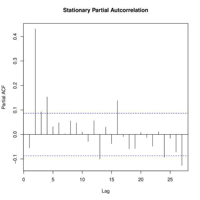
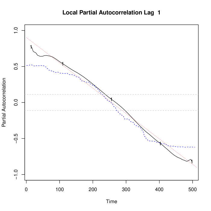
Figure 1: Partial autocorrelation function (pacf) estimators applied to a single realization of a time-varying autoregressive process. Top left: classical (stationary) pacf. Top right: Lag one local pacf. Bottom: Lag two local pacf. Theoretical: red dotted line, Daubechies D5 wavelet-based estimate ($\tilde{q}$, Section 2.4) is dashed blue line, Epanechnikov windowed estimate ($\tilde{q}_{W}$, Section 3) is solid black line. Bandwidth selected using AutoBestBW from locits package.

Unsurprisingly, the classical partial autocorrelation is misleading, indicating a significant incorrect strong lag two structure, and entirely failing to detect the existing (true) lag $1$ dependence. By contrast, our two developed local partial autocorrelation estimators correctly track the true time-dependent autoregressive parameters, thereby showing the importance of not using techniques designed for stationary series on nonstationary ones. Amongst our two proposals, the wavelet-based estimate seems a bit worse, particularly for the lag two partial autocorrelation after about time $350$. This was confirmed by a small simulation study, based on $100$ realizations drawn from the TVAR process. The average root-mean-square error for the wavelet estimator (times $10^{2}$, standard errors in parantheses) at lags one and two was $2.4(0.76)$ and $18.0(3.9)$, respectively, whereas for the windowed estimator it was $1.5(0.70)$ and $27.9(4.7)$ respectively. Both estimators are less accurate near the ends of the series, which is a common problem with such estimators, see Cheng and Hall (2003), for example. However, the windowed estimator usually appears less affected, and thus is the estimator we propose to use in practice.

The TVAR process used in Figure 1 exhibits a large range of time-varying parameter values from $-0.9$ to $+0.9$. However, we repeated the example for less extreme parameter changes. Unless the parameter change is very small, and the process is close to stationary, the classical partial autocorrelation still misleads. For smaller parameter changes, the classical partial autocorrelation often gets the process order correct, but gives a partial autocorrelation value that is often close to the average of the local partial autocorrelations.

Our second example considers a piecewise stationary AR$(p)$ process of length $T=256$. The first and last segments (each of length 85) are realizations of an AR$(1)$ process with $\phi=-0.2$, and the middle segment (of length 86) follows an AR$(2)$ process with $\phi=(0.5,0.2)$. Note the middle segment has a significantly different structure to the first and last. Our estimators correctly identify the process structure, otherwise invisible to classical approaches. This is verified by performing a small simulation study and drawing from this process 100 times. The average root-mean-square error for the wavelet estimator at lags one and two (times $10^{2}$, standard errors in parentheses) is $11\,(2)$ and $3\,(2)$, respectively, whereas for the windowed estimator it is $7\,(1)$ and $3\,(1)$ respectively. The process lag 2 structure is closer to stationarity (with corresponding true pacf 0, 0.2, 0 in the three segments) and this is reflected in the similar results for the two estimators.

4.2 U.K. National Accounts data

The ABML time series obtained from the Office for National Statistics contains values of the U.K. gross-valued added (GVA), which is a component of gross domestic product (GDP). Our ABML series is recorded quarterly from quarter one 1955 to quarter three 2010 and consists of $T=223$ observations.

Figure 2: Left: ABML time series. Right: second-order differences of ABML.

As with many economic time series, ABML exhibits a clear trend, which we removed using second-order differences; these are shown in Figure 2. Naturally, other methods for removing the trend could be tried. The second-order differences strongly suggest that the series is not second-order stationary, with the series variance increasing markedly over time. Use of methods from Nason (2013c) show that the autocorrelation also changes over time. In particular, the lag one autocorrelation undergoes a major and rapid shift around 1991.

Much of the increase in variance observed in Figure 2 is probably due to inflation. However, we have also analysed two different inflation-corrected versions of ABML, one provided by the U.K. Office of National Statistics, and both of these are also not second-order stationary, as determined by tests of stationarity in Priestley and Subba Rao (1969) and Nason (2013c).

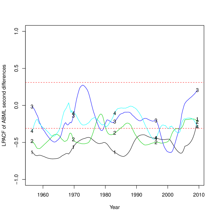
Figure 3: Windowed partial autocorrelation, $\tilde{q}_{W}(z,\tau)$, of ABML second difference series for lags one to four indicated on each curve (Epanechnikov window with $L=40$). Horizontal red dotted lines are approximate 95% confidence intervals.

Our new estimation methodology enables us to obtain the windowed local partial autocorrelation estimator, $\tilde{q}_{W}(z,\tau)$, shown in Figure 3 and computed on the ABML second-order differences. Note that crucially the local partial autocorrelation estimates within each lag ($\tau$) are time-dependent ($z$), and here these estimates suggest significant dependencies up to lag $\tau=4$. There are times, such as the 1970s, when the higher-order partial autocorrelations are not outside of the approximate significant bands, indicating that a lower lag, $2$, might be appropriate. These results are (i) economically interesting as the local variance, autocorrelation and partial autocorrelation all change over time, (ii) highlight the concerns with having no access to second-order conditional information (as was the case until now) and (iii) further pose the challenge of accurately forecasting such data. Although the topic of time series forecasting is outside the scope of this paper, many authors acknowledge the superiority of wavelet-based forecasting (Aminghafari and Poggi, 2007; Schlüter and Deuschle, 2010) and we envisage the proposed local partial autocorrelation estimator could further improve results.

4.3 Precipitation in Eastport, U.S.

Understanding precipitation patterns is important for detecting climate change indications and for policy decisions. The left panel in Figure 4 shows monthly precipitation in millimetres from January 1887 until December 1950 (768 observations) at a location in Eastport. The data can be found in Hipel and McLeod (1994) and have been analysed in many publications including Rao et al. (2012); Dhakal et al. (2015). Our windowed local partial autocorrelation estimate of the Eastport data is given in the right panel of Figure 4 and shows clear nonstationarity at lags one through three.

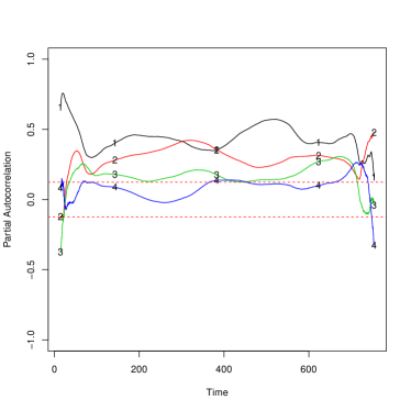
Figure 4: Left: Precipitation (mm) in Eastport, U.S. Right: Windowed partial autocorrelation, $\tilde{q}_{W}(z,\tau)$, of left for lags one to four indicated on each curve (Epanechnikov window with $L=250$, chosen by AutoBestBW from locits package.). Horizontal red dotted lines are approximate 95% confidence intervals.

Some authors analyse this series as if it were stationary and our analysis suggests that this is inappropriate. Indeed, if one applies a formal hypothesis test of nonstationarity on appropriate lengths of the series, such as that proposed by Cardinali and Nason (2018), there is strong evidence for nonstationarity. From a modelling point of view, the estimated local partial autocorrelation behaviour might support fitting a time-varying AR(3) model.

To provide some empirical support to the notion that window width is not visually critical to the interpretation of the local partial autocorrelation, Appendix H shows the smoothed local partial autocorrelation plots similar to that in the right-hand plot of Figure 4, but at three smaller window widths of 160, 80 and 40. The plot at window width of 160 is not that different to the one above at $L=250$ and, indeed, the $L=80$ plot is not that dissimilar. However, the $L=40$ plot almost certainly contains too much ‘noise’ and should be disregarded.

4.4 Euro-Dollar exchange rate

Following the introduction of the Euro currency in 1999 several authors, including Ahamada and Boutahar (2002) and Garcin (2017), have considered different properties of this series, which have an influence on setting monetary policy in various jurisdictions.

We analyze log returns of the monthly Euro-Dollar exchange rate as provided by EuroStat at
http://ec.europa.eu/eurostat/web/products-datasets/-/ei_mfrt_m
from January 1999 until October 2017. The log returns and corresponding local partial autocorrelation function estimates are given in Figure 5. This demonstrates that the log returns do not appear to be time varying (outside of the boundary locations) and exhibit only lag one partial autocorrelation. This apparent stationarity is confirmed with formal tests using the locits (Nason (2013b), Nason (2013c)) and fractal (Constantine and Percival (2016), Priestley and Subba Rao (1969)) packages in R. Interestingly this relationship holds throughout the financial crisis, from 2008 to 2011.

These examples highlight the versatility of our method and its potential use to identify stationary behaviour, manifest through local partial autocorrelation estimates that are constant through time. In addition, it highlights how the approach can identify departures from stationarity, evident through explicit time-dependent profiles at particular lags.

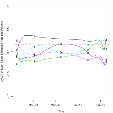
Figure 5: Left: Monthly Euro-Dollar log returns. Right: Windowed partial autocorrelation, $\tilde{q}_{W}(z,\tau)$, of left for lags one to five indicated on each curve. Horizontal red dotted lines are approximate 95% confidence intervals. (Epanechnikov window with $L=147$)

5 Discussion

This article develops two new estimators of the local partial autocorrelation function and studied their theoretical properties when applied to a locally stationary wavelet process. We established consistency for the wavelet-based estimator and asymptotic distribution for the windowed estimator. The latter result relied on new results on the integrated local wavelet periodogram, the (windowed) Haar cross-correlation wavelets and related quantities. For practical reasons, we promote the use of the windowed estimator. We demonstrated the utility of these estimators for eliciting local second-order structure on simulated data, the U.S. Eastport precipitation time series and the U.K. ABML time series. We also demonstrated the versatility of our method in the (desirable) presence of stationarity for the Euro-Dollar exchange rates. On a practical note, should the practitioner believe that higher process powers also display a locally stationary behaviour, the proposed local partial autocorrelation function could then be used to additionally uncover higher-order dependency structures. Most of the theoretical results relating to the generic local partial autocorrelation function estimator presented here are based on Haar wavelets, but many results and definitions also apply to other Daubechies’ compactly supported wavelets. The associated software package lpacf contains functionality to compute the estimators for all such wavelets, up to ten vanishing moments as contained within the wavethresh package (Nason, 2013a), as well as a cross-validation method for automatic bandwidth selection. The lpacf package will be released on to the Comprehensive R Archive Network (CRAN) in due course.

Appendix A Résumé: partial autocorrelation for stationary series

Let $\{X_{t}\}_{t\in{\mathbb{Z}}}$ be a zero-mean second-order stationary process with autocovariance function $\gamma(\tau)$. Loosely speaking, the partial autocorrelation function at lag $\tau$ is the correlation between $X_{1}$ and $X_{\tau+1}$ whilst adjusting for the “in-between” observations, $X_{2},\ldots,X_{\tau}$. Brockwell and Davis (1991, p. 54) define the closed span $\overline{\mbox{sp}}(X_{t},t\in H)$ of any subset $\{X_{t},t\in H\}$ of a Hilbert space ${\cal H}$ to be the smallest closed subspace of ${\cal H}$ which contains each $X_{t},t\in H$. Then, following Brockwell and Davis (1991, p. 98), the lag $\tau$ partial autocorrelation function $q(\tau)$ of $\{X_{t}\}$ is defined by $q(\tau)=\operatorname{corr}\left\{X_{{\tau}+1}-P_{1,\tau}(X_{{\tau+1}}),X_{1}-P_{1,\tau}(X_{{1}})\right\},$ where $P_{1,\tau}(\cdotp)$ denotes the projection operator onto $\overline{\mbox{sp}}(X_{2},\ldots,X_{\tau})$. See also Fan and Yao (2003, p. 43)

Alternatively, if $\gamma(0)>0$ and $\gamma(h)\rightarrow 0$ as $h\rightarrow\infty$, then the partial autocorrelation function, $q(\tau)$, can be obtained as the final entry of the vector $\mbox{\boldmath$\varphi$}_{\tau}$ which is the solution to the well-known Yule-Walker equations $\Gamma_{\tau}\mbox{\boldmath$\varphi$}_{\tau}=\mbox{\boldmath$\gamma$}_{\tau}$. Here $\Gamma_{\tau}=\{\gamma(i-j)\}_{i,j=1}^{\tau}$ is a $\tau\times\tau$ covariance matrix and $\mbox{\boldmath$\gamma$}_{\tau}=\{\gamma(i)\}_{i=1}^{\tau}$ is a vector of covariances. Equivalently, $q(\tau)=\varphi_{\tau,\tau}$ where $\varphi_{\tau,\tau}$ is the coefficient of $X_{1}$ when projecting $X_{\tau+1}$ on the space spanned by $X_{1},\ldots,X_{\tau}$, i.e. the projection $\hat{X}_{\tau+1}=\varphi_{\tau,1}X_{\tau}+\ldots+\varphi_{\tau,\tau}X_{1}$.

For a sampled series $\{X_{t}\}_{t=1}^{T}$, the sample partial autocorrelation at lag $\tau$ is often estimated by solving $\hat{\Gamma}_{\tau}\hat{\mbox{\boldmath$\varphi$}}_{\tau}=\hat{\mbox{\boldmath$\gamma$}}_{\tau}$, where $\hat{\gamma}$ are the usual sample autocovariances, and taking $\hat{q}(\tau):=\hat{q}_{[1,T]}(\tau)=\hat{\varphi}_{\tau,\tau}$. Here we use the index notation $[1,T]$ in order to indicate the range of observations on which the estimation of $\hat{\Gamma}_{\tau}$ and $\hat{\mbox{\boldmath$\gamma$}}_{\tau}$ is based. The properties of $\hat{q}(\cdotp)$ are well-known, see Brockwell and Davis (1991, Section 8.10). In particular, $T^{1/2}\left\{\hat{q}(\tau)-q(\tau)\right\}$ has a limiting Gaussian distribution, as $T\rightarrow\infty$, with mean zero and variance proportional to the last term on the diagonal of $\Gamma_{\tau}^{-1}$.

Appendix B Definitions of locally stationary processes

Definition 2.1 of Dahlhaus (1997) is as follows.

“A sequence of stochastic processes $X_{t,T}$ $(t=0,\ldots,T-1)$ is called locally stationary with transfer function $A^{0}$ and trend $\mu$ if there exists a representation

$$X_{t,T}=\mu(t/T)+\int_{-\pi}^{\pi}\exp(i\lambda t)A^{0}_{t,T}(\lambda)d\xi(\lambda),$$ (21)

where the following holds.

1. $\xi(\lambda)$ is a stochastic process on $[-\pi,\pi]$ with $\overline{\xi(\lambda)}=\xi(-\lambda)$ and

   $$\operatorname{cum}\{d\xi(\lambda_{1}),\ldots,d\xi(\lambda_{k})\}=\eta\left(\sum_{j=1}^{k}\lambda_{j}\right)g_{k}(\lambda_{1},\ldots,\lambda_{k-1})d\lambda_{1}\ldots d\lambda_{k},$$

   where $\operatorname{cum}\{\cdots\}$ denotes the cumulant of $k$th order, $g_{1}=0$, $g_{2}(\lambda)=1$, $|g_{k}(\lambda_{1},\ldots,\lambda_{k-1})|\leq\mbox{const}_{k}$ for all $k$ and $\eta(\lambda)=\sum_{j=-\infty}^{\infty}\delta(\lambda+2\pi j)$ is the periodic $2\pi$ extension of the Dirac delta function.

2. There exists a constant $K$ and a $2\pi$-periodic function $A:[0,1]\times{\mathbb{R}}\rightarrow{\mathbb{C}}$ with $A(u,-\lambda)=\overline{A(u,\lambda)}$ and

   $$\sup_{t,\lambda}\left|A^{0}_{t,T}(\lambda)-A\left(\frac{t}{T},\lambda\right)\right|\leq KT^{-1}$$ (22)

   for all $T$; $A(u,\lambda)$ and $\mu(u)$ are assumed to be continuous in $u$.”

Definition 1 of Nason et al. (2000), including improvements from Fryzlewicz (2003), is as follows.

“The locally stationary wavelet processes are a sequence of doubly indexed stochastic processes $\{X_{t,T}\}_{t=0,\ldots,T-1}$, $T=2^{J}\geq 1$, having the representation in the mean-square sense

$$X_{t,T}=\sum_{j=1}^{J}\sum_{k}w^{0}_{j,k;T}\psi_{j,k}(t)\xi_{j,k},$$ (23)

where $\xi_{j,k}$ is a random orthonormal increment sequence and where $\{\psi_{j,k}(t)\}_{j,k}$ is a discrete non-decimated family of wavelets based on a mother wavelet $\psi(t)$ of compact support. The quantities in (23) have the following properties:

1. ${\mathbb{E}}(\xi_{j,k})=0$ for all $j,k$. Hence $E(X_{t,T})=0$ for all $t,T$,

2. $\,{\rm cov}\left(\xi_{j,k},\xi_{\ell,m}\right)=\delta_{j,\ell}\delta_{k,m}$ where $\delta_{i,j}$ is the Kronecker delta.

3. There exists, for each $j\geq 1$ a Lipschitz continuous function $W_{j}(z)$ for $z\in(0,1)$ which fulfils the following properties:

   $$\sum_{j=1}^{\infty}|W_{j}(z)|^{2}<\infty\mbox{\ \ \ uniformly in $z\in(0,1)$};$$ (24)

   the Lipschitz constants $L_{j}$ are uniformly bounded in $j$ and

   $$\sum_{j=1}^{\infty}2^{j}L_{j}<\infty;$$ (25)

   there exists a sequence of constant $C_{j}$ such that for each $T$

   $$\sup_{k}\left|w^{0}_{j,k;T}-W_{j}(k/T)\right|\leq C_{j}/T,$$ (26)

   where $\{C_{j}\}$ fulfils $\sum_{j=1}^{\infty}C_{j}<\infty$.”

Appendix C Miscellaneous covariance matrices

The $\tau\times\tau$ covariance matrices are given by

$$\Sigma_{[zT];T}^{(b)} = \left(\begin{array}[]{ccc}\mbox{Cov}(X_{{[zT]},T},X_{{[zT]},T})&\cdots&\mbox{Cov}(X_{{[zT]},T},X_{{[zT]+\tau-1},T})\\ \vdots&\cdots&\vdots\\ \mbox{Cov}(X_{{[zT]+\tau-1},T},X_{{[zT]},T})&\cdots&\mbox{Cov}(X_{{[zT]+\tau-1},T},X_{{[zT]+\tau-1},T})\end{array}\right)$$

and

$$\Sigma_{[zT]+\tau;T}^{(f)} = \left(\begin{array}[]{ccc}\mbox{Cov}(X_{{[zT]+1},T},X_{{[zT]+1},T})&\cdots&\mbox{Cov}(X_{{[zT]+1},T},X_{{[zT]+\tau},T})\\ \vdots&\cdots&\vdots\\ \mbox{Cov}(X_{{[zT]+\tau},T},X_{{[zT]+1},T})&\cdots&\mbox{Cov}(X_{{[zT]+\tau},T},X_{{[zT]+\tau},T})\end{array}\right).$$

$$\Sigma_{[zT];T}=\left(\begin{array}[]{ccc}\mbox{Cov}(X_{{[zT]+\tau-1},T},X_{{[zT]+\tau-1},T})&\cdots&\mbox{Cov}(X_{{[zT]},T},X_{{[zT]+\tau-1},T})\\ \vdots&\cdots&\vdots\\ \mbox{Cov}(X_{{[zT]+\tau-1},T},X_{{[zT]},T})&\cdots&\mbox{Cov}(X_{{[zT]},T},X_{{[zT]},T})\end{array}\right)$$

Appendix D Cross-scale autocorrelation Haar wavelets

First note that by substituting $s=[zT]-t$ in (13) and by denoting the rectangular kernel by $h$, we obtain:

$$i_{N,z}(j,\ell,k)=\sum_{s=[zT]-N+1}^{[zT]}\psi_{j,s}\psi_{\ell,s+k-2[zT]+N/2-1}h\left(\frac{[zT]-s}{N}\right).$$ (29)

The above expression is by no means restricted to $h$ being a rectangular kernel, and other kernels may be used, as explained in the article main text.

This new formulation of $i_{N,z}$ is very similar to that of the cross-correlation wavelet $\Psi_{j,\ell}$, except that the summation limits are $[zT-N+1]$ and $[zT]$ instead of $-\infty$ and $\infty$. This similarity is true for all Daubechies’ compactly supported wavelets. We shall use this similarity to bound $i_{N,z}$ using Lemma 1.

Proposition D.1.

The cross-scale autocorrelation Haar wavelets $\Psi_{j,\ell}(\cdotp)$ at scales $\ell<j$ are given by

$$\Psi_{j,\ell}(\tau)=2^{-(j-\ell)/2}\begin{cases}0&\mbox{for }\tau<-2^{\ell},\\ -(2^{-\ell}\tau+1)&\mbox{for }-2^{\ell}\leq\tau<-2^{\ell-1},\\ 2^{-\ell}\tau&\mbox{for }-2^{\ell-1}\leq\tau<0,\\ 0&\mbox{for }0\leq\tau<2^{j-1}-2^{\ell},\\ 2^{-\ell}(2\tau-2^{j}+2^{\ell+1})&\mbox{for }2^{j-1}-2^{\ell}\leq\tau<2^{j-1}-2^{\ell-1},\\ 2^{-\ell}(2^{j}-2\tau)&\mbox{for }2^{j-1}-2^{\ell-1}\leq\tau<2^{j-1},\\ 0&\mbox{for }2^{j-1}\leq\tau<2^{j}-2^{\ell},\\ 2^{-\ell}(2^{j}-\tau-2^{\ell})&\mbox{for }2^{j}-2^{\ell}\leq\tau<2^{j}-2^{\ell-1},\\ 2^{-\ell}(\tau-2^{j})&\mbox{for }2^{j}-2^{\ell-1}\leq\tau<2^{j},\\ 0&\mbox{for }2^{j}\leq\tau.\end{cases}$$ (30)

For $\ell>j$ we have $\Psi_{j,\ell}(\tau)=\Psi_{\ell,j}(-\tau)$ and a precise formula appears in equation (31) (Appendix D). Note $\Psi_{j,j}(\tau)=\Psi_{j}(\tau)$, the regular autocorrelation wavelet.

Proof.

See Section J.1.1.

Corollary 2.

The regions on the right-hand side of (30) correspond exactly to the regions $III_{a}$ to $III_{j}$ in (79). For completeness (and usefulness in working out derived quantities) we can write down $\Psi_{j,\ell}(\tau)$ for $\ell>j$ explicitly as

$$\Psi_{j,\ell}(\tau)=2^{-(\ell-j)/2}\begin{cases}0&\mbox{for }\tau\leq-2^{\ell},\\ -2^{-j}(\tau+2^{\ell})&\mbox{for }-2^{\ell}<\tau\leq-2^{\ell}+2^{j-1},\\ 2^{-j}(2^{\ell}+\tau-2^{j})&\mbox{for }-2^{\ell}+2^{j-1}<\tau\leq-2^{\ell}+2^{j},\\ 0&\mbox{for }-2^{\ell}+2^{j}<\tau\leq-2^{\ell-1},\\ 2^{-j}(2^{\ell}+2\tau)&\mbox{for }-2^{l-1}<\tau\leq-2^{\ell-1}+2^{j-1},\\ 2^{-j}(2^{j+1}-2^{\ell}-2\tau)&\mbox{for }-2^{\ell-1}+2^{j-1}<\tau\leq-2^{\ell-1}+2^{j},\\ 0&\mbox{for }-2^{\ell-1}+2^{j}<\tau\leq 0,\\ -2^{-j}\tau&\mbox{for }0<\tau\leq 2^{j-1},\\ -(1-2^{-j}\tau)&\mbox{for }2^{j-1}<\tau\leq 2^{j}.\end{cases}$$ (31)

Appendix E Subsidiary result used in the proof of Lemma 1

Lemma 3.

For $a,b$ such that $2a,2b\in{\mathbb{N}}$ and $a,b>0$ it is the case that

$$\int_{-\pi}^{\pi}\frac{\{1-\cos(2a\omega)\}\{1-\cos(2b\omega)\}}{1-\cos(\omega)}\,d\omega=4\pi\min(a,b).$$ (32)

Proof.

See Section J.2.1.

Appendix F Additional Results Required For the Proofs from Section 3

Lemma 4.

The core function, $\Omega_{i}(u)$ for Haar wavelets is given by

$$\Omega_{i}(u)=2^{-i/2}\begin{cases}0&\mbox{for }u<-1,\\ -(u+1)&\mbox{for }-1\leq u<-\frac{1}{2},\\ u&\mbox{for }-\frac{1}{2}\leq u<0,\\ 0&\mbox{for }0\leq u<2^{i-1}-1,\\ 2u-2^{i}+2&\mbox{for }2^{i-1}-1\leq u<2^{i-1}-\frac{1}{2},\\ 2^{i}-2u&\mbox{for }2^{i-1}-\frac{1}{2}\leq u<2^{i-1},\\ 0&\mbox{for }2^{i-1}\leq u<2^{i}-1,\\ 2^{i}-u-1&\mbox{for }2^{i}-1\leq u<2^{i}-\frac{1}{2},\\ u-2^{i}&\mbox{for }2^{i}-\frac{1}{2}\leq u<2^{i},\\ 0&\mbox{for }2^{i}\leq u,\end{cases}$$ (33)

for $u\in{\mathbb{R}}$ and $i\in{\mathbb{N}}\cup\{0\}$.

Figure 6 shows a depiction of $\Omega_{i}(u)$.

Figure 6: Depiction of $\Omega_{i}(u)$. The function is symmetric about $2^{(i-1)}-\tfrac{1}{2}$ and the extent of the function is from $-1$ on the left to $2^{i}$ on the right. The width of all of the triangles is always 1 for all $i$. As $i$ increases the function gets stretched to the right (but also anchored on the left at $u=-1$), the peaks decrease in size like $2^{-i/2}$.

Proof.

See Section J.7.1.

Lemma 5.

Under the conditions and notations set out so far, for the nondecimated family of discrete Haar wavelets we have

$$T_{{\cal B}{\cal B}}(\ell,m)=\sum_{k\in{\cal B}}\sum_{n\in{\cal B}}\left\{\sum_{j=1}^{\infty}|i_{N,z}(j,\ell,k)i_{N,z}(j,m,n)|\right\}^{2}={\cal O}\{2^{2(\ell+m)}\}.$$

Proof.

See Section J.7.2.

Lemma 6.

Under the conditions and notations set out so far, for the nondecimated family of discrete Haar wavelets we have that the order of the cross terms is:

$$T_{\not{\cal B}{\cal B}}(\ell,m) =\sum_{k\not\in{\cal B}}\sum_{n\in{\cal B}}\left\{\sum_{j=1}^{\infty}|i_{N,z}(j,\ell,k)i_{N,z}(j,m,n)|\right\}^{2}={\cal O}(2^{2(\ell+m)})$$

$$T_{{\cal B}{\not\cal B}}(\ell,m) =\sum_{k\in{\cal B}}\sum_{n\not\in{\cal B}}\left\{\sum_{j=1}^{\infty}|i_{N,z}(j,\ell,k)i_{N,z}(j,m,n)|\right\}^{2}={\cal O}(2^{2(\ell+m)}).$$

Proof.

See Section J.7.3.

Lemma 7.

Under the conditions and notations set out so far, for the nondecimated family of discrete Haar wavelets we have that

$$T_{\not{{\cal B}}\not{{\cal B}}}(\ell,m)=\sum_{k\not\in{\cal B}}\sum_{n\not\in{\cal B}}\left\{\sum_{j=1}^{\infty}|i_{N,z}(j,\ell,k)i_{N,z}(j,m,n)|\right\}^{2}={\cal O}\{2^{2(\ell+m)}\}.$$

Proof.

See Section J.7.4.

Appendix G Some Exact Formulae for Haar wavelets

Fourth-order absolute value wavelet cross-correlations for Haar wavelets. In what follows we demonstrate new results on the the fourth-order absolute value wavelet cross-correlations, for Haar wavelets which were used in showing the previous results in Appendix J.5.

Recall these were defined as $B^{(r)}_{\ell}(j,i)=\sum_{p=-\infty}^{\infty}|p|^{r}|\Psi_{j,\ell}(p)\Psi_{i,\ell}(p)|$ for $r=0,1$ and scales $\ell,j,i\in{\mathbb{N}}$.

The $B$ products are symmetric in their arguments, $B^{(r)}_{\ell}(j,i)=B_{\ell}^{(r)}(i,j)$. Note that for $r=0$, for ease of notation, these $B^{(0)}$ quantities appeared as $B$ in the previous proofs.

Proposition G.1.

For Haar wavelets. (Part A) For $i,j>\ell$:

$$B^{(0)}_{\ell}(j,i)=\begin{cases}2^{-j}(2^{2\ell-1}+1)&\mbox{for $j=i$},\\ 2^{-j}(2^{2\ell-1}+1)2^{-3/2}&\mbox{for $i=j+1$},\\ 2^{-j/2}2^{-i/2}(2^{2\ell-1}+1)/6&\mbox{for $|j-i|>1$.}\end{cases}$$

Also, for all $i,j,\ell$ such that $i,j>\ell$, $B_{\ell}^{(0)}(j,i)$ is bounded by

$$B_{\ell}^{(0)}(j,i)\leq 2^{-j/2}2^{-i/2}2^{2\ell}.$$

(Part B) For $i,j<\ell$:

$$B^{(0)}_{\ell}(j,i)=\begin{cases}2^{-\ell}(2^{2j-1}+1)&\mbox{for }i=j<\ell,\\ \tfrac{3}{2}2^{-\ell}2^{-j/2}2^{5i/2-1}&\mbox{for }i<j<\ell.\end{cases}$$

(Part C) For $i<\ell<j$:

$$B^{(0)}_{\ell}(j,i)=\begin{cases}\tfrac{1}{8}2^{-(\ell+1)/2}2^{3i/2}(2^{i-\ell}+2)&\mbox{for }j=\ell+1,\\ \tfrac{1}{8}2^{-j/2}2^{3i/2}(2-2^{i-\ell})&\mbox{for }j>\ell+1.\end{cases}$$ (34)

(Part D) For $\ell=j$ and $i>\ell$:

$$B^{(0)}_{\ell}(\ell,i)=2^{-(i-\ell)/2}\begin{cases}\frac{17}{9}2^{\ell-3}&\mbox{for }i=\ell+1,\\ \frac{17}{27}2^{\ell-3}&\mbox{for }i>\ell+1.\end{cases}$$ (35)

For $i<\ell$ we have the following bound:

$$B^{(0)}_{\ell}(\ell,i)\leq 2^{3i/2}2^{-\ell/2}.$$

(Part E) Finally, when all indices are equal we can use (34) from Nason et al. (2000) to show

$$B^{(0)}_{\ell}(\ell,\ell)=\sum_{p}\Psi^{2}_{\ell}(p)=A_{\ell,\ell}=\frac{1}{3}2^{-\ell}(2^{2\ell}+5),$$

for $\ell>0$ and $A$ is the matrix from Nason et al. (2000).

The symmetry of $B$ permits evaluation of $B_{\ell}^{(0)}(j,i)$ for other orderings of $(i,j)$.

An overall bound for all $i,j,\ell$ is $B^{(0)}_{\ell}(j,i)\leq K2^{-(j+i)/2}2^{2\ell}$ for some positive constant $K$.

Proof.

See Section  K.

Appendix H LPACF of Eastport Precipitation Data at Different Window Widths

The plots below were produced by the following functions executed using the lpacf package with binwidths of 160, 80 and 40.

function(binwidth=250){
#
# Compute the Epanechnikov kernel smoothed local PACF using
# a specified binwidth, using parallel processing function
# mclapply on all points.
#
# Then plot the answer: only the first four lags
#  using colours 1 thru 4.
#
plot(lpacf.Epan(EastPortPrecip, allpoints=TRUE, binwidth=binwidth,
           ΨΨlapplyfn=mclapply), lags=1:4, lcol=1:4)
#
# Construct and plot "standard" confidence intervals
#
ci <- 1.96/sqrt(binwidth)
abline(h = c(-ci, ci), lty = 2, col = 2)
}

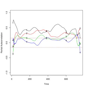
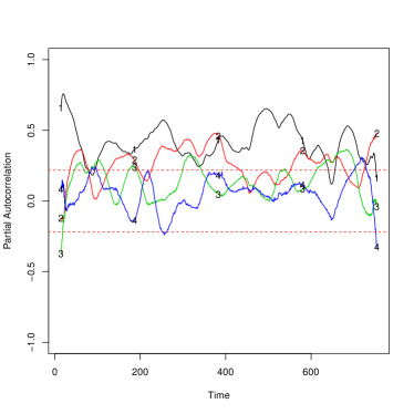
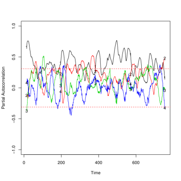
Figure 7: Windowed partial autocorrelation of Eastport Precipitation Data, $\tilde{q}_{W}(z,\tau)$, of left for lags one to four indicated on each curve. Horizontal red dotted lines are approximate 95% confidence intervals. All plots were created with the Epanechnikov window with sizes a) $L=160$, b) $L=80$, c) $L=40$.

Appendix I Proofs from Section 2.

I.1 Proof of Proposition 2.2

Proof.

We shall use the notation $P_{[zT],\tau}(X_{{[zT]},T})=\hat{X}^{(b)}_{[zT],T}$ and $P_{[zT],\tau}(X_{{[zT]+\tau},T})=\hat{X}^{(f)}_{[zT]+\tau,T}$, since these are the linear predictors of $X_{{[zT]},T}$ (back-casted), respectively $X_{{[zT]+\tau},T}$ (forecasted), using the set of predictors $X_{[zT]+1,T},\ldots,X_{[zT]+\tau-1,T}$.

Decomposing the projection space $\overline{\mbox{sp}}(X_{[zT],T},\ldots,X_{[zT]+\tau-1,T})$ into $\overline{\mbox{sp}}(X_{[zT]+1,T},$ $\ldots,$
$X_{[zT]+\tau-1,T})$ and its orthogonal complement, we can also write $\hat{X}_{[zT]+\tau,T}$ as

$$\hat{X}_{[zT]+\tau,T}=\hat{X}^{(f)}_{[zT]+\tau,T}+P^{\perp}_{[zT],\tau}(X_{{[zT]+\tau},T}),$$ (36)

where $P^{\perp}_{[zT],\tau}(\cdotp)$ denotes the projection onto the orthogonal complement space above. Since this space is $\overline{\mbox{sp}}(X_{[zT],T}-\hat{X}^{(b)}_{[zT],T})$, it then follows that $P^{\perp}_{[zT],\tau}(X_{{[zT]+\tau},T})=a(X_{{[zT]},T}-\hat{X}^{(b)}_{[zT],T})$, and using equation (36) we obtain

$$\operatorname{cov}\left(\hat{X}_{[zT]+\tau,T},X_{{[zT]},T}-\hat{X}^{(b)}_{[zT],T}\right)=a\operatorname{var}\left(X_{{[zT]},T}-\hat{X}^{(b)}_{[zT],T}\right).$$

Due to orthogonality of projection spaces, we have $\left(X_{{[zT]},T}-\hat{X}^{(b)}_{[zT],T}\right)\perp\overline{\mbox{sp}}(X_{[zT]+1,T},$ $\ldots,$ $X_{[zT]+\tau-1,T})$ and from the equation above and equation (3), it follows that $a=\varphi_{[zT],\tau,\tau;T}$.

Hence $P^{\perp}_{[zT],\tau}(X_{{[zT]+\tau},T}))=\varphi_{[zT],\tau,\tau;T}(X_{{[zT]},T}-\hat{X}^{(b)}_{[zT],T})$ and we obtain

$$\varphi_{[zT],\tau,\tau;T} = \frac{\operatorname{cov}\left(P^{\perp}_{[zT],\tau}(X_{{[zT]+\tau},T})),X_{{[zT]},T}-\hat{X}^{(b)}_{[zT],T}\right)}{\operatorname{var}\left(X_{{[zT]},T}-\hat{X}^{(b)}_{[zT],T}\right)}$$

$$= \frac{\operatorname{cov}\left({X}_{[zT]+\tau,T},X_{{[zT]},T}-\hat{X}^{(b)}_{[zT],T}\right)}{\operatorname{var}\left(X_{{[zT]},T}-\hat{X}^{(b)}_{[zT],T}\right)},$$

as $\operatorname{cov}(X_{{[zT]+\tau},T}-P^{\perp}_{[zT],\tau}(X_{{[zT]+\tau},T}),Y)=0,\forall Y\in\overline{\mbox{sp}}(X_{[zT],T}-\hat{X}^{(b)}_{[zT],T})$. Hence,

$$\varphi_{[zT],\tau,\tau;T}=\frac{\operatorname{cov}\left({X}_{[zT]+\tau,T}-\hat{X}^{(f)}_{[zT]+\tau,T},X_{{[zT]},T}-\hat{X}^{(b)}_{[zT],T}\right)}{\operatorname{var}\left(X_{{[zT]},T}-\hat{X}^{(b)}_{[zT],T}\right)}$$ (37)

because $\hat{X}^{(f)}_{[zT]+\tau,T}\perp\overline{\mbox{sp}}(X_{[zT],T}-\hat{X}^{(b)}_{[zT],T})$.

Recall from equation (1) that

$$\,q_{T}\left(z,\tau\right)=\,{\rm corr}\left(X_{{[zT]+\tau},T}-P_{[zT],\tau}(X_{{[zT]+\tau},T}),X_{[zT],T}-P_{[zT],\tau}(X_{{[zT]},T})\right),$$

or equivalently $\,q_{T}\left(z,\tau\right)=\,{\rm corr}\left(X_{{[zT]+\tau},T}-\hat{X}^{(f)}_{[zT]+\tau,T},X_{[zT],T}-\hat{X}^{(b)}_{[zT],T}\right)$ which, combined with equation (37), yields

$$\,q_{T}\left(z,\tau\right)=\varphi_{[zT],\tau,\tau;T}\left\{\frac{\operatorname{var}\left(X_{{[zT]},T}-\hat{X}^{(b)}_{[zT],T}\right)}{\operatorname{var}\left(X_{{[zT]+\tau},T}-\hat{X}^{(f)}_{[zT]+\tau,T}\right)}\right\}^{1/2}$$

as desired.

I.2 Proof of Proposition 2.3

Proof.

As $\hat{X}^{(b)}_{[zT],T}$ and $\hat{X}^{(f)}_{[zT]+\tau,T}$ are projections of $X_{{[zT]},T}$ and $X_{{[zT]+\tau},T}$, respectively, on the space $\overline{\mbox{sp}}(X_{[zT]+1,T},\ldots,X_{[zT]+\tau-1,T})$ it follows that ${\mathbb{E}}(X_{{[zT]},T}-\hat{X}^{(b)}_{[zT],T})=0$ and ${\mathbb{E}}(X_{{[zT]+\tau},T}-\hat{X}^{(f)}_{[zT]+\tau,T})=0$. Hence, the numerator and denominator in (2) can be re-expressed as a Mean Squared Prediction Error (MSPE), since

$$\operatorname{var}(X_{{[zT]},T}-\hat{X}^{(b)}_{[zT],T}) = {\mathbb{E}}(\hat{X}^{(b)}_{[zT],T}-X_{{[zT]},T})^{2}=\mbox{MSPE}(\hat{X}^{(b)}_{[zT],T},X_{{[zT]},T}),$$

$$\operatorname{var}(X_{{[zT]+\tau},T}-\hat{X}^{(f)}_{[zT]+\tau,T}) = {\mathbb{E}}(\hat{X}^{(f)}_{[zT]+\tau,T}-X_{{[zT]+\tau},T})^{2}$$

$$= \mbox{MSPE}(\hat{X}^{(f)}_{[zT]+\tau,T},X_{{[zT]+\tau},T}).$$

Using these expressions we can rewrite $\,q_{T}\left(z,\tau\right)$ from (2) as

$$\,q_{T}\left(z,\tau\right)=\varphi_{[zT],\tau,\tau;T}\left\{\frac{\mbox{MSPE}(\hat{X}^{(b)}_{[zT],T},X_{{[zT]},T})}{\mbox{MSPE}(\hat{X}^{(f)}_{[zT]+\tau,T},X_{{[zT]+\tau},T})}\right\}^{1/2}.$$

Now use the fact that the MSPE of a linear predictor of $X_{t,T}$ can be written as

$$\,\mbox{MSPE}\left(\hat{X}_{{t,T}},X_{{t,T}}\right)=\,{\mathbb{E}}\left(\hat{X}_{{t,T}}-X_{{t,T}}\right)^{2}=\mbox{\boldmath$b$}_{t}^{T}\Sigma_{t,T}\mbox{\boldmath$b$}_{t},$$

where $\mbox{\boldmath$b$}_{t}=(b_{t-1,T},\ldots,b_{0,T},-1)^{T}$ and $\Sigma_{t,T}$ is the covariance of $X_{0,T},\ldots,X_{t,T}$ (Fryzlewicz et al., 2003, Section 3.3). In our case, the back-casted and forecasted values of $X_{{[zT]},T}$ and $X_{{[zT]+\tau},T}$ are also linear predictors using the window of observations $X_{[zT]+1,T},\ldots,X_{[zT]+\tau-1,T}$, and thus their corresponding MSPE can be expressed as

$$\mbox{MSPE}(\hat{X}^{(b)}_{[zT],T},X_{{[zT]},T}) =(\mbox{\boldmath$b$}_{[zT]}^{(b)})^{T}\Sigma_{[zT];T}^{(b)}\mbox{\boldmath$b$}_{[zT]}^{(b)},$$ (38)

$$\mbox{MSPE}(\hat{X}^{(f)}_{[zT]+\tau,T},X_{{[zT]+\tau},T}) =(\mbox{\boldmath$b$}_{[zT]+\tau}^{(f)})^{T}\Sigma_{[zT]+\tau;T}^{(f)}\mbox{\boldmath$b$}_{[zT]+\tau}^{(f)},$$ (39)

where, as above, the $\tau\times 1$ coefficient vectors are $\mbox{\boldmath$b$}_{[zT]}^{(b)}=(-1,\tilde{b}^{(b)}_{1,T},\ldots,\tilde{b}^{(b)}_{{\tau-1},T})^{T}$ and $\mbox{\boldmath$b$}_{[zT]+\tau}^{(f)}=({b}^{(f)}_{\tau-2,T},\ldots,{b}^{(f)}_{0,T},-1)^{T}$ and the $\tau\times\tau$ covariance matrices $\Sigma_{[zT];T}^{(b)}$ and $\Sigma_{[zT]+\tau;T}^{(f)}$ appear in Appendix C.

Therefore, on combining equation (4) with (38) and (39) we obtain as desired

$$\,q_{T}\left(z,\tau\right)=\varphi_{[zT],\tau,\tau;T}\left\{\frac{(\mbox{\boldmath$b$}_{[zT]}^{(b)})^{T}\Sigma_{[zT];T}^{(b)}\mbox{\boldmath$b$}_{[zT]}^{(b)}}{(\mbox{\boldmath$b$}_{[zT]+\tau}^{(f)})^{T}\Sigma_{[zT]+\tau;T}^{(f)}\mbox{\boldmath$b$}_{[zT]+\tau}^{(f)}}\right\}^{1/2}.$$

I.3 Proof of Proposition 2.5

Proof.

The proof treats the convergence of $\varphi_{[zT],\tau,\tau;T}$ and the quotient that forms the square-root in equation (4) separately. Firstly, we address the quotient convergence.

A: Quotient Convergence: By Proposition 3.1 from Fryzlewicz et al. (2003) we have

$$\,\mbox{MSPE}\left(\hat{X}_{[zT],T}^{(b)},X_{[zT],T}\right)=(\mbox{\boldmath$b$}_{[zT]}^{(b)})^{T}\Sigma_{[zT];T}^{(b)}\mbox{\boldmath$b$}_{[zT]}^{(b)}=\left\{(\mbox{\boldmath$b$}_{[zT]}^{(b)})^{T}{\rm B}_{[zT]}^{(b)}\mbox{\boldmath$b$}_{[zT]}^{(b)}\right\}\left\{1+o_{T}(1)\right\}$$

and

$$\,\mbox{MSPE}\left(\hat{X}_{{[zT]+\tau,T}}^{(f)},X_{{[zT]+\tau,T}}\right) = (\mbox{\boldmath$b$}_{[zT]+\tau}^{(f)})^{T}\Sigma_{[zT]+\tau;T}^{(f)}\mbox{\boldmath$b$}_{[zT]+\tau}^{(f)}$$

$$= \left\{(\mbox{\boldmath$b$}_{[zT]+\tau}^{(f)})^{T}{\rm B}_{[zT]+\tau}^{(f)}\mbox{\boldmath$b$}_{[zT]+\tau}^{(f)}\right\}\left\{1+o_{T}(1)\right\}.$$

Hence

$$\frac{\,\mbox{MSPE}\left(\hat{X}_{[zT],T}^{(b)},X_{[zT],T}\right)}{\,\mbox{MSPE}\left(\hat{X}_{[zT]+\tau,T}^{(f)},X_{[zT]+\tau,T}\right)}=\frac{\left\{(\mbox{\boldmath$b$}_{[zT]}^{(b)})^{T}{\rm B}_{[zT]}^{(b)}\mbox{\boldmath$b$}_{[zT]}^{(b)}\right\}}{\left\{(\mbox{\boldmath$b$}_{[zT]+\tau}^{(f)})^{T}{\rm B}_{[zT]+\tau}^{(f)}\mbox{\boldmath$b$}_{[zT]+\tau}^{(f)}\right\}}\left\{1+o_{T}(1)\right\}$$

B: Convergence of $\varphi_{[zT],\tau,\tau;T}$. We defined $\varphi_{[zT],\tau,\tau;T}$ as the last element in $\mbox{\boldmath$\varphi$}_{[zT],\tau;T}$ that is the solution to the Yule-Walker equations $\Sigma_{[zT];T}\mbox{\boldmath$\varphi$}_{[zT],\tau;T}=\,\mbox{\boldmath$r$}_{[zT];T}$.

Let $[{\mathcal{O}}(T^{-1})]$ be an appropriately-sized matrix whose elements are all ${\mathcal{O}}(T^{-1})$ and ${\mathcal{O}}(T^{-1})$ be a similarly defined vector.

Now consider

$$\Sigma_{[zT];T}\left(\mbox{\boldmath$\varphi$}_{[zT],\tau;T}-\mbox{\boldmath$\varphi$}_{[zT],\tau}\right) =\Sigma_{[zT];T}\mbox{\boldmath$\varphi$}_{[zT],\tau;T}-\Sigma_{[zT];T}\mbox{\boldmath$\varphi$}_{[zT],\tau}$$

$$=\,\mbox{\boldmath$r$}_{[zT];T}-\left({\rm B}_{[zT]}+[{\mathcal{O}}(T^{-1})]\right)\mbox{\boldmath$\varphi$}_{[zT],\tau}$$

$$=\,\mbox{\boldmath$r$}_{[zT];T}-\,\mbox{\boldmath$r$}_{[zT]}-[{\mathcal{O}}(T^{-1})]\mbox{\boldmath$\varphi$}_{[zT],\tau} |c_{T}(z,\tau)-c(z,\tau)|={\mathcal{O}}(T^{-1})$$ (as )

$$=\mbox{\boldmath${\mathcal{O}}(T^{-1})$}-[{\mathcal{O}}(T^{-1})]\mbox{\boldmath$\varphi$}_{[zT],\tau}.$$

Observe that $[{\mathcal{O}}(T^{-1})]\mbox{\boldmath$\varphi$}_{[zT],\tau}=\left(\sum_{j}\sum_{i}K_{j,i}\varphi_{[zT],\tau,j}/T\right)\mbox{\boldmath$1$}$, where $K_{j,i}$ is the $(j,i)$th constant, and in what follows we shall seek to bound this quantity.

From the Cauchy-Schwarz inequality $\|\mbox{\boldmath$\varphi$}_{[zT],\tau}\|_{1}\leq|\tau|^{1/2}\|\mbox{\boldmath$\varphi$}_{[zT],\tau}\|_{2}=C_{\tau}$ as $\tau$ is fixed, and by standard properties of the spectral norm

$$\|\mbox{\boldmath$\varphi$}_{[zT],\tau}\|_{2}^{2} =\mbox{\boldmath$\varphi$}_{[zT],\tau}^{T}\mbox{\boldmath$\varphi$}_{[zT],\tau}$$

$$\leq\mbox{\boldmath$\varphi$}_{[zT],\tau}^{T}\Sigma_{[zT];T}\mbox{\boldmath$\varphi$}_{[zT],\tau}\|\Sigma_{[zT];T}^{-1}\|$$

$$=\,\mbox{MSPE}\left(\hat{X}_{{[zT]+\tau-1,T}},X_{{[zT]+\tau-1,T}}\right)\|\Sigma_{[zT];T}^{-1}\|<\infty,$$

as the spectral norm $\|\Sigma_{[zT];T}^{-1}\|$ is bounded using Lemma A.3 from Fryzlewicz et al. (2003).

Thus $[{\mathcal{O}}(T^{-1})]\mbox{\boldmath$\varphi$}_{[zT],\tau}=\mbox{\boldmath${\mathcal{O}}(T^{-1})$}$ and it follows that

$$\Sigma_{[zT];T}\left(\mbox{\boldmath$\varphi$}_{[zT],\tau;T}-\mbox{\boldmath$\varphi$}_{[zT],\tau}\right)=\mbox{\boldmath${\mathcal{O}}(T^{-1})$},$$

which is equivalent to $\mbox{\boldmath$\varphi$}_{[zT],\tau;T}-\mbox{\boldmath$\varphi$}_{[zT],\tau}=\Sigma_{[zT];T}^{-1}\mbox{\boldmath${\mathcal{O}}(T^{-1})$}$. By bounds of Rayleigh quotients (Abadir and Magnus, 2005, pg.181), $\|\mbox{\boldmath$\varphi$}_{[zT],\tau;T}-\mbox{\boldmath$\varphi$}_{[zT],\tau}\|_{2}$ $=\|\Sigma_{[zT];T}^{-1}\mbox{\boldmath${\mathcal{O}}(T^{-1})$}\|_{2}$ $\leq\mu^{1/2}\|\mbox{\boldmath${\mathcal{O}}(T^{-1})$}\|_{2}$ $=(\mu|\tau|)^{1/2}/T$ $={\mathcal{O}}(T^{-1})$ as $\tau$ is fixed. Here $\mu$ is the largest eigenvalue of $\left(\Sigma_{[zT];T}^{-1}\right)^{T}\Sigma_{[zT];T}^{-1}$, i.e. $\mu=\|\Sigma_{[zT];T}^{-1}\|^{2}$, and so $\mu<\infty$. It follows that $\mbox{\boldmath$\varphi$}_{[zT],\tau;T}-\mbox{\boldmath$\varphi$}_{[zT],\tau}=\mbox{\boldmath${\mathcal{O}}(T^{-1})$}$.

Putting parts A and B together:

$$\left|\,q_{T}\left(z,\tau\right)-\,q\left(z,\tau\right)\right| =\left|\varphi_{[zT],\tau,\tau;T}\left\{\frac{\,\mbox{MSPE}\left(\hat{X}_{{[zT],T}}^{(b)},X_{{[zT],T}}\right)}{\,\mbox{MSPE}\left(\hat{X}_{[zT]+\tau,T}^{(f)},X_{[zT]+\tau,T}\right)}\right\}^{1/2}\right.$$

$$\left.-\varphi_{[zT],\tau,\tau}\left\{\frac{(\mbox{\boldmath$b$}_{[zT]}^{(b)})^{T}{\rm B}_{[zT]}^{(b)}\mbox{\boldmath$b$}_{[zT]}^{(b)}}{(\mbox{\boldmath$b$}_{[zT]+\tau}^{(f)})^{T}{\rm B}_{[zT]+\tau}^{(f)}\mbox{\boldmath$b$}_{[zT]+\tau}^{(f)}}\right\}^{1/2}\right|$$

$$\begin{split}&=\left|\left\{\varphi_{[zT],\tau,\tau}+{\mathcal{O}}(T^{-1})\right\}\right.\\ &\left.\left[\frac{\left\{(\mbox{\boldmath$b$}_{[zT]}^{(b)})^{T}{\rm B}_{[zT]}^{(b)}\mbox{\boldmath$b$}_{[zT]}^{(b)}\right\}\left\{1+o_{T}(1)\right\}}{\left\{(\mbox{\boldmath$b$}_{[zT]+\tau}^{(f)})^{T}{\rm B}_{[zT]+\tau}^{(f)}\mbox{\boldmath$b$}_{[zT]+\tau}^{(f)}\right\}\left\{1+o_{T}(1)\right\}}\right]^{1/2}\right.\\ &\qquad\left.-\varphi_{[zT],\tau,\tau}\left\{\frac{(\mbox{\boldmath$b$}_{[zT]}^{(b)})^{T}{\rm B}_{[zT]}^{(b)}\mbox{\boldmath$b$}_{[zT]}^{(b)}}{(\mbox{\boldmath$b$}_{[zT]+\tau}^{(f)})^{T}{\rm B}_{[zT]+\tau}^{(f)}\mbox{\boldmath$b$}_{[zT]+\tau}^{(f)}}\right\}^{1/2}\right|\end{split}$$

$$\begin{split}&=\left|\varphi_{[zT],\tau,\tau}\left\{\frac{(\mbox{\boldmath$b$}_{[zT]}^{(b)})^{T}{\rm B}_{[zT]}^{(b)}\mbox{\boldmath$b$}_{[zT]}^{(b)}}{(\mbox{\boldmath$b$}_{[zT]+\tau}^{(f)})^{T}{\rm B}_{[zT]+\tau}^{(f)}\mbox{\boldmath$b$}_{[zT]+\tau}^{(f)})}\right\}^{1/2}\right.\\ &\left.\left(\left[\frac{\left\{1+o_{T}(1)\right\}}{\left\{1+o_{T}(1)\right\}}\right]^{1/2}-1\right)\right.\\ &\qquad\left.+{\mathcal{O}}(T^{-1})\left\{\frac{\,\mbox{MSPE}\left(\hat{X}_{[zT],T}^{(b)},X_{[zT],T}\right)}{\,\mbox{MSPE}\left(\hat{X}_{[zT]+\tau,T}^{(f)},X_{[zT]+\tau,T}\right)}\right\}^{1/2}\right|\end{split}$$

$$={\mathcal{O}}(T^{-1}).$$

For the last equality the first term is asymptotically zero since $\frac{\left\{1+o_{T}(1)\right\}}{\left\{1+o_{T}(1)\right\}}\to 1$ as $T\to\infty$, $\varphi_{[zT],\tau,\tau}<\infty$ and

$$\left\{(\mbox{\boldmath$b$}_{[zT]}^{(b)})^{T}{\rm B}_{[zT]}^{(b)}\mbox{\boldmath$b$}_{[zT]}^{(b)}\right\}^{1/2}\left\{(\mbox{\boldmath$b$}_{[zT]+\tau}^{(f)})^{T}{\rm B}_{[zT]+\tau}^{(f)}\mbox{\boldmath$b$}_{[zT]+\tau}^{(f)}\right\}^{-1/2}<\infty,$$

or, more concisely, $\,q\left(z,\tau\right)<\infty$. The second term is ${\mathcal{O}}(T^{-1})$ as each expectation is finite. This concludes the proof.

I.4 Proof of Proposition 2.7

Proof.

First recall that we defined the local partial autocorrelation as

$$\,q\left(z,\tau\right)=\varphi_{[zT],\tau,\tau;T}\left\{\frac{\mbox{Var}\{X_{[zT],T}-P_{[zT],\tau}(X_{{[zT]},T})\}}{\mbox{Var}\{X_{{[zT]+\tau},T}-P_{[zT],\tau}(X_{{[zT]+\tau},T})\}}\right\}^{1/2},$$

where the coefficient $\varphi_{[zT],\tau,\tau;T}$ is obtained in a manner akin to the (stationary) partial autocorrelation coefficient by expressing $X_{[zT]+\tau,T}$ as an $\mbox{AR}(\tau)$ process and solving the associated Yule-Walker equations. The fraction under the square root quantifies the ratio between the backward and forward variances associated to the $\mbox{AR}(\tau)$ process. The Yule-Walker equations here are localized at the rescaled time $z$, in the sense that they involve observations over the interval $\left[[zT],[zT]+\tau\right]$.

Recall that, in estimating the local partial autocorrelation, we use the $\hat{c}(z,\tau)$ estimator of Nason et al. (2000), which was shown there to be consistent for the (true) local autocovariance ${c}(z,\tau)$. By the classical stationary theory, it follows that the estimated Yule-Walker coefficients of the $\mbox{AR}(\tau)$ process (solution vector to the local Yule-Walker equations) are consistent estimators of the true coefficients, hence $\tilde{\varphi}_{[zT],\tau,\tau;T}\overset{P}{\longrightarrow}\varphi_{[zT],\tau,\tau}$, and the forward and backward variances are also estimated consistently.

Using the continuous mapping theorem (Billingsley, 1999) and assuming that the variance is non-zero, it follows that the square-root of the ratio of estimated backward and forward variances

$$\left\{\frac{(\,\tilde{\mbox{\boldmath$b$}}_{[zT]}^{(b)})^{T}\,\tilde{{\rm B}}_{[zT]}^{(b)}\,\tilde{\mbox{\boldmath$b$}}_{[zT]}^{(b)}}{(\,\tilde{\mbox{\boldmath$b$}}_{[zT]+\tau}^{(f)})^{T}\,\tilde{{\rm B}}_{[zT]+\tau}^{(f)}\,\tilde{\mbox{\boldmath$b$}}_{[zT]+\tau}^{(f)}}\right\}^{1/2}$$

is a consistent estimator of the true ratio of variances

$$\left\{\frac{(\mbox{\boldmath$b$}_{[zT]}^{(b)})^{T}{\rm B}_{[zT]}^{(b)}\mbox{\boldmath$b$}_{[zT]}^{(b)}}{(\mbox{\boldmath$b$}_{[zT]+\tau}^{(f)})^{T}{\rm B}_{[zT]+\tau}^{(f)}\mbox{\boldmath$b$}_{[zT]+\tau}^{(f)}}\right\}^{1/2}.$$

This together with the consistency of $\tilde{\varphi}_{[zT],\tau,\tau;T}$, yields

$$\begin{split}\tilde{\varphi}_{[zT],\tau,\tau;T}\left\{\frac{(\,\tilde{\mbox{\boldmath$b$}}_{[zT]}^{(b)})^{T}\,\tilde{{\rm B}}_{[zT]}^{(b)}\,\tilde{\mbox{\boldmath$b$}}_{[zT]}^{(b)}}{(\,\tilde{\mbox{\boldmath$b$}}_{[zT]+\tau}^{(f)})^{T}\,\tilde{{\rm B}}_{[zT]+\tau}^{(f)}\,\tilde{\mbox{\boldmath$b$}}_{[zT]+\tau}^{(f)}}\right\}^{1/2}\overset{P}{\longrightarrow}\\ \varphi_{[zT],\tau,\tau}\left\{\frac{(\mbox{\boldmath$b$}_{[zT]}^{(b)})^{T}{\rm B}_{[zT]}^{(b)}\mbox{\boldmath$b$}_{[zT]}^{(b)}}{(\mbox{\boldmath$b$}_{[zT]+\tau}^{(f)})^{T}{\rm B}_{[zT]+\tau}^{(f)}\mbox{\boldmath$b$}_{[zT]+\tau}^{(f)}}\right\}^{1/2}.\end{split}$$ (40)

Appendix J Proofs from Section 3.

J.1 Cross-scale autocorrelation Haar wavelets

J.1.1 Proof of Proposition D.1

Proof.

For completeness, the definition of (continuous-time) Haar wavelets is

$$\psi_{H}(x)=\begin{cases}-1&\mbox{if }0\leq x<1/2,\\ 1&\mbox{if }1/2\leq x<1,\\ 0&\mbox{otherwise.}\end{cases}$$

Nason et al. (2000) show that $\Psi_{j}(\tau)=\Psi_{H}(2^{-j}|\tau|)$ where $\Psi_{j}(\tau)$ is the regular discrete autocorrelation wavelet and $\Psi_{H}(u)$ is the continuous Haar autocorrelation wavelet given by

$$\Psi_{H}(u)=\int_{-\infty}^{\infty}\psi_{H}(x)\psi_{H}(x-u)\,dx=\ \begin{cases}1-3|u|&\mbox{for }|u|\in[0,\frac{1}{2}],\\ |u|-1&\mbox{for }|u|\in(\frac{1}{2},1].\end{cases}$$

Hence, we can derive the following integral equation for $\Psi_{j}(\tau)$ for $\tau\geq 0$:

$$\Psi_{j}(\tau)=\Psi_{H}(2^{-j}\tau)=\int_{-\infty}^{\infty}\psi_{H}(x)\psi_{H}(x-2^{-j}\tau)\,dx$$

from the definition of $\Psi_{H}(u)$. Then make the substitution $x=2^{-j}y$ to obtain:

$$\Psi_{j}(\tau) =\int_{-\infty}^{\infty}\psi_{H}(2^{-j}y)\psi_{H}(2^{-j}y-2^{-j}\tau)\,2^{-j}\,dy$$

$$=\int_{-\infty}^{\infty}2^{-j/2}\psi_{H}(2^{-j}y)\,2^{-j/2}\psi_{H}\{2^{-j}(y-\tau)\}\,dy$$

$$=\int_{-\infty}^{\infty}\psi_{j,0}(y)\psi_{j,0}(y-\tau)\,dy,$$

where $\psi_{j,0}(y)=2^{-j/2}\psi_{H}(2^{-j}y)$.

Hence, by a similar argument it is the case that

$$\Psi_{j,\ell}(\tau)=\int_{-\infty}^{\infty}\psi_{j,0}(y)\psi_{\ell,0}(y-\tau)\,dy.$$

For Haar wavelets, since we know the precise form of $\psi_{H}$ we should be able to obtain an analytical formula for $\Psi_{j,\ell}$. To do this we consider $\ell<j$ and see that

$$\Psi_{j,\ell}(\tau)=\int_{-\infty}^{\infty}2^{-j/2}\psi_{H}(2^{-j}y)2^{-\ell/2}\psi_{H}\{2^{-\ell}(y-\tau)\}\,dy.$$

Now let $x=2^{-\ell}y$ and we obtain

$$\Psi_{j,\ell}(\tau) =\int_{-\infty}^{\infty}2^{-j/2}\psi_{H}\{2^{-(j-\ell)}x\}2^{\ell/2}\psi_{H}(x-2^{-\ell}\tau)\,dx$$

$$=\int_{-\infty}^{\infty}\psi_{j-\ell}(x)\psi(x-2^{-\ell}\tau)\,dx.$$

Hence, it makes sense to introduce the following core function:

$$\Omega_{i}(u)=\int_{-\infty}^{\infty}\psi_{i}(x)\psi(x-u)\,dx,$$

for integers $i=0,1,2,\ldots$. Clearly,

$$\Psi_{j,\ell}(\tau)=\Omega_{j-\ell}(2^{-\ell}\tau),$$ (41)

for $\ell<j$. Also $\Omega_{0}(u)=\Psi_{H}(u)$.

Using Lemma 4 and (41), we can now specify an exact formula for $\Psi_{j,\ell}(\tau)$. For $\ell<j$ the result is shown in (30). Corollary 2 shows the formula for $\ell>j$.

Proposition D.1 shows that the support of the cross-correlation wavelet is $\{k\in{\mathbb{Z}}:-2^{\ell}<=k<2^{j}\}$ for $\ell<j$.

J.2 Subsidiary result used in the proof of Lemma 1

J.2.1 Proof of Lemma 3

Proof.

The result is obtained by combining known results on the Fejér and Dirichlet kernels as follows. The Fejér kernel can be defined by:

$$F_{n}(\omega)=\frac{\sin^{2}(n\omega/2)}{2\pi n\sin^{2}(\omega/2)}=\frac{1-\cos(n\omega)}{2\pi n\{1-\cos(\omega)\}},$$

for $\omega\in[-\pi,\pi]$, see Walter and Shen (2000) Section 4.2, for example. The Fejér kernel can also be written in the following alternative form

$$F_{n}(\omega)=\frac{1}{n}\sum_{k=0}^{n-1}D_{k}(\omega),$$ (42)

where $D_{k}(\omega)=\pi^{-1}\left(\frac{1}{2}+\sum_{p=1}^{k}\cos p\omega\right)$ is the Dirichlet kernel, see Section 1.2.1 of Walter and Shen (2000).

Let the integral on the left-hand side of (32) be $I1$. Then:

$$I1 =2\pi\int_{-\pi}^{\pi}\{1-\cos(2a\omega)\}2bF_{2b}(\omega)\,d\omega$$

$$=4\pi b\left\{\int_{-\pi}^{\pi}F_{2b}(\omega)\,d\omega-\int_{-\pi}^{\pi}\cos(2a\omega)F_{2b}(\omega)\,d\omega\right\}$$

$$=4\pi b\left\{1-\int_{-\pi}^{\pi}\cos(2a\omega)(2b)^{-1}\sum_{k=0}^{2b-1}D_{k}(\omega)\,d\omega\right\},$$

by substituting (42) and since $\int_{-\pi}^{\pi}F_{n}(\omega)\,d\omega=1$. Then

$$I1 =4\pi b\left\{1-(2b)^{-1}\sum_{k=0}^{2b-1}\int_{-\pi}^{\pi}\cos(2a\omega)D_{k}(\omega)\,d\omega\right\}$$

$$=4\pi b\{1-(2b)^{-1}\sum_{k=0}^{2b-1}I2_{k}\},$$ (43)

where $I2_{k}=\int_{-\pi}^{\pi}D_{k}(\omega)\cos(2a\omega)\,d\omega$. Now,

$$I2_{k} =\pi^{-1}\int_{-\pi}^{\pi}\left(\frac{1}{2}+\sum_{p=1}^{k}\cos p\omega\right)\cos(2a\omega)\,d\omega$$

$$=(2\pi)^{-1}\int_{-\pi}^{\pi}\cos(2a\omega)\,d\omega+\pi^{-1}\sum_{p=1}^{k}\int_{-\pi}^{\pi}\cos(p\omega)\cos(2a\omega)\,d\omega$$ (44)

$$=(2\pi)^{-1}\left[\frac{\sin(2a\omega)}{2a}\right]_{-\pi}^{\pi}+\pi^{-1}\sum_{p=1}^{k}\left[\frac{2a\cos(p\omega)\sin(2a\omega)-p\cos(2a\omega)\sin(p\omega)}{4a^{2}-p^{2}}\right]_{-\pi}^{\pi}$$

$$=0,$$ (45)

for $p^{2}\neq 4a^{2}$ for $p\neq 2a$ (and recall $a>0$). For $p=2a$ the integral in (44) is

$$\int_{-\pi}^{\pi}\cos^{2}(2a\omega)\,d\omega=\pi+\sin(4a\pi)/4a=\pi,$$ (46)

since $2a\in{\mathbb{N}}$. Hence,

$$I2_{k}=\begin{cases}0&\mbox{for }k<2a\\ 1&\mbox{for }k\geq 2a.\end{cases}$$ (47)

Hence, substituting (47) into (43) gives, for $b>a$

$$I1=4\pi b\{1-(2b)^{-1}(2b-2a)\}\\ =4\pi b-2\pi(2b-2a)\\ =4\pi a.$$ (48)

Since the integral (32) is symmetric in $a$ and $b$ we also have $I1=4\pi b$ for $b\leq a$. Hence, the result in equation (32) follows.

J.3 Proof of Lemma 1

Proof.

It is obvious that inequality (14) holds when $i_{N,z}(j,\ell,k)=0$. This occurs when the lower limit in the sum (13), plus the extra $k-2[zT]+N/2-1$ exceeds the support of $\psi_{\ell,\cdot}$. In other words, $i_{N,z}(j,\ell,k)=0$ when:

$$[zT]-N+1+k-2[zT]+N/2-1>N_{\ell}-1$$

$$\implies k-[zT]-N/2>N_{\ell}-1$$

$$\implies k>[zT]+N/2+N_{\ell}-1=b_{2}.$$ (49)

It can also be shown that $i_{N,z}(j,\ell,k)=0$ when $k<[zT]-N/2+1$ but this inequality is not of interest in this proof .

For the inequalities in (15) we decompose $\Psi$ into three terms:

$$\Psi_{j,\ell}(k-2[zT]+N/2-1)=L+i_{N,z}(j,\ell,k)+U,$$ (50)

where

$$L=\sum_{s=-\infty}^{[zT]-N}\psi_{j,s}\psi_{\ell,s+k-2[zT]+N/2-1}$$ (51)

and

$$U=\sum_{s=[zT]+1}^{\infty}\psi_{j,s}\psi_{\ell,s+k-2[zT]+N/2-1}.$$ (52)

Clearly, the inequality (14) is satisfied when $i_{N,z}(j,\ell,k)=\Psi_{j,\ell}(k-2[zT]+N/2-1)$ which occurs when $L=U=0$. We now investigate the conditions when $L=U=0$.

(A) When is $U=0$? When the lower limit of the sum defining $U$ in (52) exceeds the support of $\psi_{j,\cdot}$, i.e.

$$[zT]+1>N_{j}-1\implies[zT]>N_{j}-2,$$ (53)

or when the lower limit exceeds the support of $\psi_{\ell,\cdot}$, i.e.

$$[zT]+1+k-2[zT]+N/2-1>N_{\ell}-1\implies k>[zT]-N/2+N_{\ell}-1.$$ (54)

(B) When is $L=0$? When the upper limit of the sum defining $L$ in (51) is less than the lower support bound of $\psi_{j,\cdot}$, which is zero, i.e.

$$[zT]-N<0\implies[zT]<N,$$ (55)

or when the upper limit is less than the support of $\psi_{\ell,\cdot}$, i.e.

$$[zT]-N+k-2[zT]+N/2-1<0\implies k<[zT]+N/2+1=b_{1}.$$ (56)

Hence, $U=L=0$ when inequalities (53) and (56) are satisfied. Note: we are not particularly interested in inequalities (54) and (55). For the former, the inequality (54) would have to be allied with (55) (as (56) would be contradictory to (54)) and, asymptotically (55) will not hold (as we expect the rate of increase of $T$ to be much bigger than $N$).

So far we have demonstrated the Lemma up to inequalities (15) and (16) and now we look to establish the second part of the Lemma.

To establish (17) it can be shown that, for Daubechies’ wavelets with two or more vanishing moments,

$$|i_{N,z}(j,\ell,k)| \leq 2^{-(j+\ell)/2}K^{2}\sum_{s=[zT]-N+1}^{[zT]}s^{-1}(s-[zT]+N)^{-1}$$ (57)

$$=2^{-(j+\ell)/2}\left(\mathcal{H}_{N}-\mathcal{H}_{[zT]}+\mathcal{H}_{[zT]-N}\right)/([zT]-N),$$

where $\mathcal{H}_{n}$ is the $n$th Harmonic number, and $K$ is a constant (maximum absolute value of the wavelet). Now using the following approximation for $\mathcal{H}_{n}$

$$\mathcal{H}_{n}=\log n+\gamma+{\mathcal{O}}(n^{-1}),$$

where $\gamma$ is the Euler-Mascheroni constant, we can obtain the result in (17).

Now we consider Haar wavelets. First, let us recall what the discrete Haar wavelet is. We have

$$\psi_{j,k}=\begin{cases}2^{-j/2}&\mbox{for }0\leq k<N_{j}/2,\\ -2^{-j/2}&\mbox{for }N_{j}/2\leq k<N_{j},\\ 0&\mbox{otherwise.}\end{cases}$$

For Haar wavelets $N_{j}=2^{j}$ for $j\in{\mathbb{N}}$. Next we will require the discrete Fourier transform of the Haar wavelet given by:

$$\hat{\psi}_{j}(\omega)=\sum_{s=-\infty}^{\infty}\psi_{j,s}e^{-i\omega s},$$

for $\omega\in(-\pi,\pi)$. The inverse of this transform is:

$$\psi_{j,s}=(2\pi)^{-1}\int_{-\pi}^{\pi}\hat{\psi}_{j}(\omega)e^{i\omega s}d\omega$$ (58)

for $s\in{\mathbb{Z}}$.

Now let us work out the precise form of the Fourier transform of the discrete Haar wavelet:

$$\hat{\psi}_{j}(\omega) =2^{-j/2}\left(\sum_{s=0}^{N_{j}/2-1}e^{-i\omega s}-\sum_{s=N_{j}/2}^{N_{j}-1}e^{-i\omega s}\right)$$

$$=2^{-j/2}\left\{\sum_{s=0}^{N_{j}/2-1}e^{-i\omega s}-\sum_{s=0}^{N_{j}/2-1}e^{-i\omega(s+N_{j}/2)}\right\}$$

$$=2^{-j/2}\sum_{s=0}^{N_{j}/2-1}e^{-i\omega s}\left(1-e^{-i\omega N_{j}/2}\right)$$

$$=2^{-j/2}\left(1-e^{-i\omega N_{j}/2}\right)\sum_{s=0}^{N_{j}/2-1}e^{-i\omega s}$$

$$=2^{-j/2}\left(1-e^{-i\omega N_{j}/2}\right)\frac{1-\exp(-i\omega N_{j}/2)}{1-\exp(-i\omega)}$$

$$=2^{-j/2}\frac{\left(1-e^{-i\omega N_{j}/2}\right)^{2}}{1-\exp(-i\omega)}$$

We now directly examine formula (29) with a rectangular kernel, as discussed in the main body of the paper. To simplify notation, we let $B=[zT]-N$ and $r=k-2[zT]+N/2-1$. In (29) replace the discrete wavelets $\psi_{j,s}$ and $\psi_{\ell,s+r}$ by their Fourier inverse representations given by (58) to obtain:

$$i_{N,z}(j,\ell,k) =\sum_{s=B+1}^{B+N}(2\pi)^{-2}\int_{-\pi}^{\pi}\int_{-\pi}^{\pi}\hat{\psi}_{j}(\omega)e^{i\omega s}\hat{\psi}_{\ell}(\nu)e^{i\nu(s+r)}d\omega d\nu$$ (59)

$$=(2\pi)^{-1}\int_{-\pi}^{\pi}\hat{\psi}_{\ell}(\nu)e^{i\nu r}\left\{(2\pi)^{-1}\times\right.$$ (60)

$$\left.\hskip 85.35826pt\int_{-\pi}^{\pi}\hat{\psi}_{j}(\omega)\sum_{s=B+1}^{B+N}e^{i(\omega+\nu)s}d\omega\right\}d\nu$$ (61)

$$=(2\pi)^{-1}\int_{-\pi}^{\pi}\hat{\psi}_{\ell}(\nu)e^{i\nu r}\left\{(2\pi)^{-1}\times\right.$$ (62)

$$\left.\hskip 85.35826pt\int_{-\pi}^{\pi}\hat{\psi}_{j}(\omega)e^{i(\omega+\nu)(B+1)}\frac{1-e^{i(\omega+\nu)N}}{1-e^{i(\omega+\nu)}}d\omega\right\}d\nu$$

$$=(2\pi)^{-1}\int_{-\pi}^{\pi}\hat{\psi}_{\ell}(\nu)e^{i\nu r}G_{j,B,N}(\nu)d\nu,$$ (63)

where

$$G_{j,B,N}(\nu) =(2\pi)^{-1}\int_{-\pi}^{\pi}\hat{\psi}_{j}(\omega)e^{i(\omega+\nu)(B+1)}\frac{1-e^{i(\omega+\nu)N}}{1-e^{i(\omega+\nu)}}d\omega$$

$$=\sum_{s=B+1}^{B+N}e^{i\nu s}\psi_{j,s}$$

$$=\hat{\psi}_{j}(\nu)-\sum_{s=-\infty}^{B}\psi_{j,s}e^{i\nu s}-\sum_{s=B+N+1}^{\infty}\psi_{j,s}e^{i\nu s}.$$

We now examine what happens to $G_{j,B,N}(\nu)$ under four different cases depending on how the support of the wavelet $\psi_{j,s}$ overlaps the interval $[B+1,B+N]$ or not. Note: the support of the wavelet is the interval $[0,N_{j}-1]$. Note: we are mostly interested in the situation when $T,N$ are large and hence not so interested in a potential fifth case when $[B+1,B+N]\subseteq[0,N_{j}-1]$.

Case-I: Suppose $[0,N_{j}-1]\subseteq[B+1,B+N]$. That is, the support of the wavelet lies entirely within the interval $[B+1,B+N]$. Then

$$G_{j,B,N}(\nu)=\sum_{s=B+1}^{B+N}e^{i\nu s}\psi_{j,s}=\sum_{s=0}^{N_{j}-1}\psi_{j,s}e^{i\nu s}=\hat{\psi}_{j}(\nu).$$ (64)

Case-II: Suppose $0<B+1$ but $B+1<N_{j}-1$, that is right-hand end of the wavelet support overlaps $[B+1,B+N]$ but the left-hand end does not. Then:

$$G_{j,B,N}(\nu) =\sum_{s=B+1}^{N_{j}-1}\psi_{j,s}e^{i\nu s}=\hat{\psi}_{j}(\nu)-\sum_{s=0}^{B}\psi_{j,s}e^{i\nu s}$$ (65)

$$=\hat{\psi}_{j}(\nu)-G_{j,B}(\nu),$$ (66)

where

$$G_{j,B}(\nu)=\sum_{s=0}^{B}\psi_{j,s}e^{i\nu s}.$$ (67)

Case-III: Suppose $[0,N_{j}-1]$ and $[B,B+N]$ do not overlap. Then $G_{j,B,N}(\nu)=0$.

Case-IV: Suppose that $0<B+N$ and $B+N<N_{j}-1$, that is the left-hand end of the wavelet support overlaps $[B+1,B+N]$ but the right-hand end does not. And $B+1<0$ which is not of interest as it means that $[zT]-N+1<0$ which should not happen, for large $T$, as $T$ increases faster than $N$.

Now let us derive $G_{j,B}(\nu)$ from (67) for $B>0$:

$$G_{j,B}(\nu)=\begin{cases}2^{-j/2}\sum_{s=0}^{B}e^{i\nu s}&\mbox{if }0\leq B\leq N_{j}/2-1,\\ 2^{-j/2}\left(\sum_{s=0}^{N_{j}/2-1}e^{i\nu s}-\sum_{s=N_{j}/2}^{B}e^{i\nu s}\right)&\mbox{if }N_{j}/2-1<B\leq N_{j}-1,\\ 2^{-j/2}\sum_{s=0}^{N_{j}/2-1}\left\{e^{i\nu s}-e^{i\nu(s+N_{j}/2)}\right\}&\mbox{if }N_{j}-1<B.\end{cases}$$ (68)

Computing the sums in (68) gives:

$$G_{j,B}(\nu)=\frac{2^{-j/2}}{\{\exp(i\nu)-1\}}\begin{cases}\exp\{i\nu(B+1)\}-1,&\text{for $B\in S_{1}$,}\\ 2\exp(i\nu N_{j}/2)-\exp\{i\nu(B+1)\}-1,&\text{for $B\in S_{2}$},\\ \{1-\exp(i\nu N_{j}/2)\}\{\exp(i\nu N_{j}/2)-1\},&\text{for $B\in S_{3}$},\end{cases}$$ (69)

where $S_{1}=\{B:0\leq B\leq N_{j}/2-1\},S_{2}=\{B:N_{j}/2-1<B\leq N_{j}-1\},S_{3}=\{B:N_{j}-1<B\}$.

Now returning to the main formula (59).

Case-I: suppose $[0,N_{j}-1]\subseteq[B+1,B+N]$ then $G_{j,B,N}(\nu)=\hat{\psi}_{j}(\nu)$ as given by (64). Hence, substituting into (59) gives:

$$i_{N,z}(j,\ell,k) =(2\pi)^{-1}\int_{-\pi}^{\pi}\hat{\psi}_{\ell}(\nu)e^{i\nu r}G_{j,B,N}(\nu)\,d\nu$$ (70)

$$=(2\pi)^{-1}\int_{-\pi}^{\pi}2^{-\ell/2}\frac{(1-e^{-i\nu N_{\ell}/2})^{2}}{1-e^{-i\nu}}e^{i\nu r}2^{-j/2}\frac{(1-e^{-i\nu N_{j}/2})^{2}}{1-e^{-i\nu}}\,d\nu$$

$$=\frac{2^{-(j+\ell)/2}}{2\pi}\int_{-\pi}^{\pi}e^{i\nu r}\frac{(1-e^{-i\nu N_{\ell}/2})^{2}(1-e^{-i\nu N_{j}/2})^{2}}{(1-e^{-i\nu})^{2}}\,d\nu$$ (71)

We now bound $i_{N,z}(j,\ell,k)$ by the integral of the absolute value of its integrand, i.e.

$$|i_{N,z}(j,\ell,k)| \leq\frac{2^{-(j+\ell)/2}}{2\pi}\int_{-\pi}^{\pi}\frac{2\{1-\cos(N_{\ell}\nu/2)\}2\{1-\cos(N_{j}\nu/2)\}}{2\{1-\cos(\nu)\}}\,d\nu$$

$$=\frac{2^{1-(j+\ell)/2}}{2\pi}\int_{-\pi}^{\pi}\frac{\{1-\cos(N_{\ell}\nu/2)\}\{1-\cos(N_{j}\nu/2)\}}{1-\cos(\nu)}\,d\nu,$$

because $|e^{i\nu r}|=1$, $|(1-e^{-i\nu})|^{2}=2\{1-\cos(\nu)\}$, and so on. Using Lemma 3 with $a=N_{\ell}/4,b=N_{j}/4$ gives

$$|i_{N,z}(j,\ell,k)| \leq 2^{-(j+\ell)/2}\min(N_{\ell},N_{j})$$ (72)

$$=\begin{cases}2^{-(j-\ell)/2}&\mbox{ for $\ell\leq j$},\\ 2^{-(\ell-j)/2}&\mbox{ for $\ell>j$},\end{cases}$$ (73)

as $N_{j}=2^{j}$ for Haar wavelets.

Case-IIa. Consider the case when $0\leq B\leq N_{j}/2-1$. From (66) we have $G_{j,B,N}(\nu)=\hat{\psi}_{j}(\nu)-G_{j,B}(\nu)$. Hence:

$$i_{N,z}(j,\ell,k) \leq\frac{1}{2\pi}\int_{-\pi}^{\pi}\hat{\psi}_{\ell}(\nu)e^{i\nu r}G_{j,B,N}(\nu)\,d\nu$$

$$=\frac{1}{2\pi}\int_{-\pi}^{\pi}\hat{\psi}_{\ell}(\nu)e^{i\nu r}\left[\hat{\psi}_{j}(\nu)-G_{j,B}(\nu)\right]\,d\nu$$

$$=\frac{1}{2\pi}\int_{-\pi}^{\pi}\hat{\psi}_{\ell}(\nu)e^{i\nu r}\hat{\psi}_{j}(\nu)\,d\nu$$

$$-\frac{1}{2\pi}\int_{-\pi}^{\pi}\hat{\psi}_{\ell}(\nu)e^{i\nu r}\frac{2^{j/2}}{e^{i\nu}-1}\left[e^{i\nu(B+1)}-1\right]\,d\nu$$

$$=\eqref{eqn:CaseIpremod}-\frac{2^{-(j+\ell)/2}}{2\pi}\int_{-\pi}^{\pi}\frac{\left(1-e^{-i\nu N_{\ell}/2}\right)^{2}\left(1-e^{i\nu(B+1)}\right)e^{i\nu r}}{\left(1-e^{i\nu}\right)\left(1-e^{-i\nu}\right)}\,d\nu$$

$$\leq\eqref{eqn:CaseIpremod}-\frac{2^{-(j+\ell)/2}}{2\pi}\int_{-\pi}^{\pi}\frac{\left(1-e^{-i\nu N_{\ell}/2}\right)^{2}\left(1-e^{i\nu N_{j}/2}\right)e^{i\nu r}}{\left(1-e^{i\nu}\right)\left(1-e^{-i\nu}\right)}\,d\nu$$

We now bound $i_{N,z}(j,\ell,k)$ by the integral of the absolute value of its integrand, i.e.

$$|i_{N,z}(j,\ell,k)| \leq\eqref{eq:case1end}+\frac{2^{-(j+\ell)/2}}{2\pi}\int_{-\pi}^{\pi}\frac{|\left(1-e^{-i\nu N_{\ell}/2}\right)^{2}||\left(1-e^{i\nu N_{j}/2}\right)||e^{i\nu r}|}{|\left(1-e^{i\nu}\right)\left(1-e^{-i\nu}\right)|}\,d\nu$$

$$\leq\eqref{eq:case1end}+\frac{2^{-(j+\ell)/2}}{2\pi}\int_{-\pi}^{\pi}\frac{2\left(1-\cos(\nu N_{\ell}/2)\right)2}{2\left(1-\cos(\nu)\right)}\,d\nu$$

$$=\eqref{eq:case1end}+\frac{2^{-(j+\ell)/2}}{\pi}\int_{-\pi}^{\pi}2\pi(N_{\ell}/2)F_{N_{\ell}/2}(\nu)\,d\nu$$

$$=\eqref{eq:case1end}+2^{-(j+\ell)/2}N_{\ell}$$

$$=2^{-(j+\ell)/2}\left(\min(N_{\ell},N_{j})+N_{\ell}\right),$$

Case-IIb. Consider the case when $N_{j}/2-1<B\leq N_{j}-1$. Again using (66) we have $G_{j,B,N}(\nu)=\hat{\psi}_{j}(\nu)-G_{j,B}(\nu)$ and from the corresponding value of (69), we obtain (based on the same logic as above in Cases I and IIa):

$$i_{N,z}(j,\ell,k) \leq\frac{1}{2\pi}\int_{-\pi}^{\pi}\hat{\psi}_{\ell}(\nu)e^{i\nu r}G_{j,B,N}(\nu)\,d\nu$$

$$=\frac{1}{2\pi}\int_{-\pi}^{\pi}\hat{\psi}_{\ell}(\nu)e^{i\nu r}\left[\hat{\psi}_{j}(\nu)-G_{j,B}(\nu)\right]\,d\nu$$

$$=\eqref{eqn:CaseIpremod}-\frac{1}{2\pi}\int_{-\pi}^{\pi}\hat{\psi}_{\ell}(\nu)e^{i\nu r}\frac{2^{j/2}}{e^{i\nu}-1}\left[2e^{i\nu N_{j}/2}-e^{i\nu(B+1)}-1\right]\,d\nu$$

$$\leq\eqref{eqn:CaseIpremod}-\frac{1}{2\pi}\int_{-\pi}^{\pi}\hat{\psi}_{\ell}(\nu)e^{i\nu r}\frac{2^{j/2}}{e^{i\nu}-1}\left[2e^{i\nu N_{j}/2}-e^{i\nu N_{j}}-1\right]\,d\nu$$

$$=\eqref{eqn:CaseIpremod}$$

$$+\frac{2^{-(j+\ell)/2}}{2\pi}\int_{-\pi}^{\pi}\frac{\left(1-e^{-i\nu N_{\ell}/2}\right)^{2}\left(2e^{i\nu N_{j}/2}-1-e^{i\nu N_{j}}\right)e^{i\nu r}}{\left(1-e^{i\nu}\right)\left(1-e^{-i\nu}\right)}\,d\nu$$

We now bound $i_{N,z}(j,\ell,k)$ by the integral of the absolute value of its integrand, i.e.

$$|i_{N,z}(j,\ell,k)| \leq\eqref{eq:case1end}$$

$$+\frac{2^{-(j+\ell)/2}}{2\pi}\int_{-\pi}^{\pi}\frac{|\left(1-e^{-i\nu N_{\ell}/2}\right)^{2}||\left(1-2e^{i\nu N_{j}/2}+e^{i\nu N_{j}}\right)||e^{i\nu r}|}{|\left(1-e^{i\nu}\right)\left(1-e^{-i\nu}\right)|}\,d\nu$$

$$\leq\eqref{eq:case1end}+\frac{2^{-(j+\ell)/2}}{2\pi}\int_{-\pi}^{\pi}\frac{2\left(1-\cos(\nu N_{\ell}/2)\right)2}{2\left(1-\cos(\nu)\right)}\,d\nu$$

$$=\eqref{eq:case1end}+\frac{2^{1-(j+\ell)/2}}{\pi}\int_{-\pi}^{\pi}\pi(N_{\ell}/2)F_{N_{\ell}/2}(\nu)\,d\nu$$

$$=\eqref{eq:case1end}+2^{-(j+\ell)/2}N_{\ell}$$

$$=2^{-(j+\ell)/2}\left(\min(N_{\ell},N_{j})+N_{\ell}\right),$$

Case-III. Clearly, $|i_{N,z}(j,\ell,k)|\leq 0\leq\eqref{eq:case1end}$ and Case-IV does not apply.

J.4 Proof of Lemma 2

This lemma has two parts, hence we next prove the first part.

Proof.

In what follows we use the two bounds (14) for $k<b_{1}$ and $k>b_{2}$ and (18) for $b_{1}\leq k\leq b_{2}$ from Lemma 1. Denote ${\cal B}=[b_{1},b_{2}]$ and express

$$\sum_{k=-\infty}^{\infty}\sum_{j=1}^{\infty}{\arrowvert}i_{N,z}(j,\ell,k){\arrowvert}^{2} =\sum_{k\in{\cal B}}\sum_{j=1}^{\infty}{\arrowvert}i_{N,z}(j,\ell,k){\arrowvert}^{2}+\sum_{k\in\not{\cal B}}\sum_{j=1}^{\infty}{\arrowvert}i_{N,z}(j,\ell,k){\arrowvert}^{2}.$$

For the first sum:

$$\sum_{k\in{\cal B}}\sum_{j=1}^{\infty}{\arrowvert}i_{N,z}(j,\ell,k){\arrowvert}^{2} \leq\sum_{k\in{\cal B}}\sum_{j=1}^{\infty}2^{-(j+\ell)}\left(\min(N_{\ell},N_{j})+N_{\ell}\right)^{2}$$

$$=\sum_{k\in{\cal B}}\left\{\sum_{j=1}^{\ell-1}2^{-(j+\ell)}\left(N_{j}+N_{\ell}\right)^{2}+\sum_{j=\ell}^{\infty}2^{-(j+\ell)}\left(2N_{\ell}\right)^{2}\right\}$$

$$=2^{-\ell}\sum_{k\in{\cal B}}\left\{\sum_{j=1}^{\ell-1}2^{-j}\left(2^{2j}+2^{2\ell}+2^{1+j+\ell}\right)+4\sum_{j=\ell}^{\infty}2^{-j}2^{2\ell}\right\}$$

$$=2^{-\ell}\sum_{k\in{\cal B}}\left\{\sum_{j=1}^{\ell-1}2^{j}+2^{2\ell}\sum_{j=1}^{\ell-1}2^{-j}\right.$$

$$\hskip 113.81102pt\left.+2^{1+\ell}\sum_{j=1}^{\ell-1}1+2^{2+2\ell}\sum_{j=\ell}^{\infty}2^{-j}\right\}$$

$$=2^{-\ell}\sum_{k\in{\cal B}}\left\{2^{\ell}-2+2^{2\ell}\left(1-2^{-\ell+1}\right)\right.$$

$$\hskip 113.81102pt\left.+\left(\ell-1\right)2^{1+\ell}+2^{2+2\ell}2^{-\ell+1}\right\}$$

$$=\left(N_{\ell}-1\right)2^{-\ell}\left\{\left(2\ell+5\right)2^{\ell}-2+2^{2\ell}\right\}$$

$$=\left(N_{\ell}-1\right)\left(2\ell+5-2^{-\ell+1}+2^{\ell}\right)$$

$$=\mathcal{O}\left(2^{2\ell}\right).$$

For the second sum:

$$\sum_{k\in\not{\cal B}}\sum_{j=1}^{\infty}{\arrowvert}i_{N,z}(j,\ell,k){\arrowvert}^{2} \leq\sum_{k\in\not{\cal B}}\sum_{j=1}^{\infty}|\Psi_{j,\ell}\left(k-2[zT]+N/2-1\right)|^{2}$$

$$\leq\sum_{j}B_{\ell}(j,j),$$

where $B_{\ell}(j,p)$ is the fourth-order cross-correlation wavelet absolute value product of order $r=0$, defined as $B^{(r)}_{\ell}(j,i)=\sum_{p=-\infty}^{\infty}|p|^{r}|\Psi_{j,\ell}(p)\Psi_{i,\ell}(p)|$ for $r=0,1$ and scales $\ell,j,i\in{\mathbb{N}}$.

Splitting the sum of $j$ and using Proposition G.1 leads to the following:

$$\sum_{j}B_{\ell}(j,j) =\sum_{j=0}^{\ell-1}B_{\ell}(j,j)+\sum_{j=\ell+1}^{\infty}B_{\ell}(j,j)+B_{\ell}(\ell,\ell)$$

$$=\sum_{j=0}^{\ell-1}2^{-\ell}\left(2^{2j-1}+1\right)+\sum_{j=\ell+1}^{\infty}2^{-j}\left(2^{2\ell-1}+1\right)+\frac{1}{3}2^{-\ell}\left(2^{2\ell}+5\right)$$

$$=2^{-\ell}\left[\frac{1}{2}\frac{1}{3}\left(2^{2\ell}-1\right)+\ell\right]+\left(2^{2\ell-1}+1\right)2^{-\ell}+\frac{1}{3}2^{-\ell}\left(2^{2\ell}+5\right)$$

$$=\mathcal{O}\left(2^{\ell}\right).$$

Hence $\sum_{k=-\infty}^{\infty}\sum_{j=1}^{\infty}{\arrowvert}i_{N,z}(j,\ell,k){\arrowvert}^{2}={\mathcal{O}}(2^{2\ell})$.

Now we prove the second part of Lemma 2.

Proof.

Consider

$$\sum_{k=-\infty}^{\infty}\sum_{n=-\infty}^{\infty} \left\{\sum_{j=1}^{\infty}{\arrowvert}i_{N,z}(j,\ell,k)i_{N,z}(j,m,n){\arrowvert}\right\}^{2}$$

$$=\sum_{k}\sum_{n}\sum_{j=1}^{\infty}|i_{N,z}(j,\ell,k)i_{N,z}(j,m,n)|\times$$

$$\hskip 113.81102pt\sum_{p=1}^{\infty}|i_{N,z}(p,\ell,k)i_{N,z}(p,m,n)|$$

$$=\sum_{j,p=1}^{\infty}\sum_{k}|i_{N,z}(j,\ell,k)i_{N,z}(p,\ell,k)|\sum_{n}|i_{N,z}(j,m,n)i_{N,z}(p,m,n)|$$

$$\begin{split}&=\sum_{j,p=1}^{\infty}\left\{\sum_{k\in{\cal B}}|i_{N,z}(j,\ell,k)i_{N,z}(p,\ell,k)|\right.\\ &\left.\hskip 113.81102pt+\sum_{k\not\in{\cal B}}|i_{N,z}(j,\ell,k)i_{N,z}(p,\ell,k)|\right\}\\ &\quad\times\left\{\sum_{n\in{\cal B}}|i_{N,z}(j,m,n)i_{N,z}(p,m,n)|\right.\\ &\left.\hskip 113.81102pt+\sum_{n\not\in{\cal B}}|i_{N,z}(j,m,n)i_{N,z}(p,m,n)|\right\}\end{split}$$

$$=T_{{\cal B}{\cal B}}(j,\ell,p,m)+T_{{\cal B}{\not{\cal B}}}(j,\ell,p,m)+T_{\not{\cal B}{{\cal B}}}(j,\ell,p,m)+T_{\not{\cal B}{\not{\cal B}}}(j,\ell,p,m).$$

The term $T_{\not{\cal B}\not{\cal B}}=\sum_{k\not\in{\cal B}}\sum_{n\not\in{\cal B}}$ is the case where $i_{N,z}$ can be bounded by $\Psi$ and is addressed in detail in Lemma 7. The term $T_{{\cal B}{\cal B}}=\sum_{k\in{\cal B}}\sum_{n\in{\cal B}}$ is dealt with in Lemma 5 using the bound (18) for $i_{N,z}$ from Lemma 1 and the cross term is dealt with in Lemma 6. Each of these lemmas (below) show that each of the product terms is of order no worse than ${\cal O}\{2^{2(\ell+m)}\}$.

J.5 Proof of Theorem 1

Proof.

First recall that we are under the zero-mean locally stationary wavelet process framework as described in Appendix B, with $\{X_{t,T}\}_{t=0}^{T-1}$ a doubly-index stochastic process with representation given by

$$X_{t,T}=\sum_{j=1}^{\infty}\sum_{k=-\infty}^{\infty}w^{0}_{j,k;T}\psi_{j,k}(t)\xi_{j,k}.$$

The integrated local periodogram was defined as

$$J_{N}(z,\phi)=\sum_{j=1}^{\infty}\phi_{j}I^{\ast}_{N}(z,j)$$

where $\{\phi_{j}\}_{j=1}^{\infty}\in\Phi$, with $\Phi$ a set of complex-valued bounded sequences equipped with uniform norm $||\phi||_{\infty}:=\sup_{j}|\phi_{j}|$ and in order to avoid notational clutter $N$ replaces the interval length notation $L(T)$ present in the main body of the paper. The quantity $I^{\ast}_{N}(z,j)$ denotes the uncorrected tapered local wavelet periodogram

$$I^{\ast}_{N}(z,j)=H_{N}^{-1}\left|\sum_{t=0}^{N-1}h\left(\frac{t}{N}\right)X_{t-N/2+1,T}\psi_{j,[zT]}(t)\right|^{2},$$

with $h:[0,1]\rightarrow{\mathbb{R}}_{+}$ a data taper, $H_{N}:=\sum_{j=0}^{N-1}h^{2}(j/N)\sim N\int_{0}^{1}h^{2}(x)\,dx$ the normalizing factor and $h(\cdotp)$ is assumed symmetric and with a bounded second derivative.

As in Dahlhaus and Giraitis (1998) we approximate $J_{N}(z,\phi)$ by the corresponding statistics of a stationary process with the same local corresponding statistics at $t=zT$, $z$ fixed. Let

$$J^{Y}_{N}(\phi)=\sum_{j=1}^{\infty}\phi_{j}I^{\ast,Y}_{N}(j)$$

where

$$I^{\ast,Y}_{N}(j):=H_{N}^{-1}\left|\sum_{s=0}^{N-1}h\left(\frac{s}{N}\right)Y_{[zT]-N/2+1+s,T}\psi_{j,[zT]}(s)\right|^{2}$$

is the wavelet periodogram on the segment $[zT]-N/2+1,\ldots,[zT]+N/2$ of the stationary process

$$Y_{s}=\sum_{j=1}^{\infty}W_{j}(z)\sum_{k=-\infty}^{\infty}\psi_{j,k}(s)\xi_{j,k}.$$

Note: The next section uses sequences of bounded variation The total variation of a sequence $\{\phi_{j}\}_{j=1}^{\infty}$ is defined by $\operatorname{TV}(\{\phi_{j}\})=\sum_{j=1}^{\infty}|\phi_{j+1}-\phi_{j}|$ and the space of all sequences of finite total variation is denoted by $\operatorname{bv}$, see Dunford and Schwartz (1958) for example.

From equations (11) and (12), we obtain $J_{N}(z,\phi)-{\mathbb{E}}\left(J_{N}(z,\phi)\right)=J^{Y}_{N}(\phi)-{\mathbb{E}}\left(J^{Y}_{N}(\phi)\right)+o_{p}(N^{-1/2})$ and using equation (10) it follows that

$$J_{N}(z,\phi)=J^{Y}_{N}(\phi)+{\mathcal{O}}\left(N^{-1}\right)+o_{p}(N^{-1/2})$$

which reveals the approximation we make and should be compared to equation (4.4) in Dahlhaus and Giraitis (1998), where a term ${\mathcal{O}}\left(\frac{N}{T}\right)$ appears instead of ${\mathcal{O}}\left(N^{-1}\right)$.

Using the uncorrected tapered local periodogram expression in equation (8) and the LSW definition in equation (23), by rearranging formulae we can write the integrated wavelet periodogram:

$$J_{N}(z,\phi)=\sum_{\ell=1}^{\infty}\sum_{k=-\infty}^{\infty}\sum_{m=1}^{\infty}\sum_{n=-\infty}^{\infty}\hat{d}_{N,z}(\ell,k,m,n)\xi_{\ell,k}\xi_{m,n},$$

where

$$\hat{d}_{N,z}(\ell,k,m,n)=H_{N}^{-1}w^{0}_{\ell,k}w^{0}_{m,n}\sum_{j=1}^{\infty}\phi_{j}i_{N,z}(j,\ell,k)i_{N,z}(j,m,n)$$

and from (29)

$$i_{N,z}(j,\ell,k)=\sum_{t=0}^{N-1}h\left(\frac{t}{N}\right)\psi_{j,[zT]-t}\psi_{\ell,k-[zT]-t-1+N/2}.$$

Using the properties of the $\{\xi_{\ell,k}\}_{\ell,k}$ field, we obtain

$${\mathbb{E}}\{J_{N}(z,\phi)\} =\sum_{\ell=1}^{\infty}\sum_{k=-\infty}^{\infty}\sum_{m=1}^{\infty}\sum_{n=-\infty}^{\infty}\hat{d}_{N,z}(\ell,k,m,n)\delta_{l,m}\delta_{k,n}$$

$$=\sum_{\ell=1}^{\infty}\sum_{k=-\infty}^{\infty}\hat{d}_{N,z}(\ell,k,\ell,k)$$

$$\begin{split}&=\sum_{\ell=1}^{\infty}\sum_{k=-\infty}^{\infty}H_{N}^{-1}\left[\left\{w^{0}_{\ell,k}-W_{\ell}(k/T)\right\}+\left\{W_{\ell}(k/T)-W_{\ell}(z)\right\}\right.\\ &\hskip 85.35826pt\left.+W_{\ell}(z)\right]^{2}\sum_{j=1}^{\infty}\phi_{j}{\arrowvert}i_{N,z}(j,\ell,k){\arrowvert}^{2}\end{split}$$

$$=\underbrace{\sum_{\ell=1}^{\infty}\sum_{k=-\infty}^{\infty}H_{N}^{-1}W_{\ell}^{2}(z)\sum_{j=1}^{\infty}\phi_{j}{\arrowvert}i_{N,z}(j,\ell,k){\arrowvert}^{2}}_{{\mathbb{E}}(J_{N}^{Y}(\phi))}+\mbox{ cross terms},$$

where the assumption $\sum_{j}W_{j}(z)^{2}2^{2j}<\infty$ (at any rescaled time $z$) ensures that ${\mathbb{E}}(J_{N}^{Y}(\phi))$ is finite.

Therefore, using the LSW property that $\sup_{k}\left|w^{0}_{\ell,k;T}-W_{\ell}(k/T)\right|\leq C_{\ell}/T$, leads to

$${\arrowvert}{\mathbb{E}}\{J_{N}(z,\phi)\}-{\mathbb{E}}\{J^{Y}_{N}(\phi)\}{\arrowvert}\leq\mbox{ sum of the modulus of the cross terms,}$$

all upper bounded by terms of the form

$$A =\frac{{\Arrowvert}\phi{\Arrowvert}}{H_{N}}\sum_{\ell=1}^{\infty}\sum_{k=-\infty}^{\infty}\frac{C_{\ell}^{2}}{T^{2}}\sum_{j=1}^{\infty}{\arrowvert}i_{N,z}(j,\ell,k){\arrowvert}^{2},$$

$$B =\frac{{\Arrowvert}\phi{\Arrowvert}}{H_{N}}\sum_{\ell=1}^{\infty}\sum_{k=-\infty}^{\infty}\left[\frac{C_{\ell}}{T}\left\{W_{\ell}(k/T)-W_{\ell}(z)\right\}\sum_{j=1}^{\infty}{\arrowvert}i_{N,z}(j,\ell,k){\arrowvert}^{2}\right],$$

$$C =\frac{{\Arrowvert}\phi{\Arrowvert}}{H_{N}}\sum_{\ell=1}^{\infty}\sum_{k=-\infty}^{\infty}\left[\left\{W_{\ell}(k/T)-W_{\ell}(z)\right\}^{2}\sum_{j=1}^{\infty}{\arrowvert}i_{N,z}(j,\ell,k){\arrowvert}^{2}\right],$$

$$D =\frac{{\Arrowvert}\phi{\Arrowvert}}{H_{N}}\sum_{\ell=1}^{\infty}\sum_{k=-\infty}^{\infty}\left[\left\{W_{\ell}(k/T)-W_{\ell}(z)\right\}W_{\ell}(z)\sum_{j=1}^{\infty}{\arrowvert}i_{N,z}(j,\ell,k){\arrowvert}^{2}\right].$$

In order to further bound these quantities, we use Lemma 2 that proves

$$\sum_{k=-\infty}^{\infty}\sum_{j=1}^{\infty}{\arrowvert}i_{N,z}(j,\ell,k){\arrowvert}^{2}={\mathcal{O}}(2^{2\ell}),$$

hence we obtain

$$A=\frac{{\Arrowvert}\phi{\Arrowvert}}{H_{N}}\sum_{\ell=1}^{\infty}\sum_{k=-\infty}^{\infty}\frac{C_{\ell}^{2}}{T^{2}}\sum_{j=1}^{\infty}{\arrowvert}i_{N,z}(j,\ell,k){\arrowvert}^{2} =\frac{{\Arrowvert}\phi{\Arrowvert}}{H_{N}}\sum_{\ell=1}^{\infty}\frac{C_{\ell}^{2}}{T^{2}}\sum_{k=-\infty}^{\infty}\sum_{j=1}^{\infty}{\arrowvert}i_{N,z}(j,\ell,k){\arrowvert}^{2}$$

$$\leq\frac{{\Arrowvert}\phi{\Arrowvert}}{H_{N}}\frac{1}{T^{2}}\sum_{\ell=1}^{\infty}C_{\ell}^{2}2^{2\ell}={\mathcal{O}}(N^{-1}T^{-2}),$$

where we have used $\sum_{\ell=1}^{\infty}C_{\ell}^{2}2^{2\ell}<\infty$.

$$B =\frac{{\Arrowvert}\phi{\Arrowvert}}{H_{N}}\sum_{\ell=1}^{\infty}\sum_{k=-\infty}^{\infty}\left[\frac{C_{\ell}}{T}\left\{W_{\ell}(k/T)-W_{\ell}(z)\right\}\sum_{j=1}^{\infty}{\arrowvert}i_{N,z}(j,\ell,k){\arrowvert}^{2}\right]$$

$$\leq\frac{{\Arrowvert}\phi{\Arrowvert}}{H_{N}}\sum_{\ell=1}^{\infty}\sum_{k=-\infty}^{\infty}\sum_{j=1}^{\infty}\frac{C_{\ell}}{T}L_{\ell}\left|\frac{k-[zT]}{T}\right|{\arrowvert}i_{N,z}(j,\ell,k){\arrowvert}^{2}$$

$$\leq\frac{{\Arrowvert}\phi{\Arrowvert}}{H_{N}}\frac{1}{T}\sum_{\ell=1}^{\infty}C_{\ell}L_{\ell}2^{2\ell}={\mathcal{O}}(N^{-1}T^{-1}),$$

using the Lipschitz continuity of $\{W_{j}\}_{j}$, $T^{-1}{\arrowvert}k-[zT]{\arrowvert}\in(0,1)$ and the Hölder inequality

$$\sum_{\ell=1}^{\infty}C_{\ell}L_{\ell}2^{2\ell}<\left(\sum_{\ell=1}^{\infty}C_{\ell}^{2}2^{2\ell}\right)^{1/2}\left(\sum_{\ell=1}^{\infty}L_{\ell}^{2}2^{2\ell}\right)^{1/2}<\infty$$

coupled with the assumptions in the theorem.

We now need to bound

$$C =\frac{{\Arrowvert}\phi{\Arrowvert}}{H_{N}}\sum_{\ell=1}^{\infty}\sum_{k=-\infty}^{\infty}\left[\left\{W_{\ell}(k/T)-W_{\ell}(z)\right\}^{2}\sum_{j=1}^{\infty}{\arrowvert}i_{N,z}(j,\ell,k){\arrowvert}^{2}\right]$$

$$\leq\frac{{\Arrowvert}\phi{\Arrowvert}}{H_{N}}\sum_{\ell=1}^{\infty}\sum_{k=-\infty}^{\infty}\sum_{j=1}^{\infty}L_{\ell}^{2}\frac{{\arrowvert}(k-[zT])^{2}{\arrowvert}}{T^{2}}{\arrowvert}i_{N,z}(j,\ell,k){\arrowvert}^{2}.$$

As $\sum_{\ell}L_{\ell}^{2}2^{2\ell}<\infty$ and as ${\arrowvert}\frac{k-[zT]}{T}{\arrowvert}^{2}\in(0,1)$, we obtain that $C={\mathcal{O}}(N^{-1})$.

The term

$$D =\frac{{\Arrowvert}\phi{\Arrowvert}}{H_{N}}\sum_{\ell=1}^{\infty}\sum_{k=-\infty}^{\infty}\left[\left\{W_{\ell}(k/T)-W_{\ell}(z)\right\}W_{\ell}(z)\sum_{j=1}^{\infty}{\arrowvert}i_{N,z}(j,\ell,k){\arrowvert}^{2}\right]$$

$$\leq\frac{{\Arrowvert}\phi{\Arrowvert}}{H_{N}}\sum_{\ell=1}^{\infty}\sum_{k=-\infty}^{\infty}\sum_{j=1}^{\infty}L_{\ell}W_{\ell}(z)\frac{{\arrowvert}(k-[zT]){\arrowvert}}{T}{\arrowvert}i_{N,z}(j,\ell,k){\arrowvert}^{2}$$

can be bounded using Hölder’s inequality

$$\sum_{\ell=1}^{\infty}W_{\ell}(z)L_{\ell}2^{2\ell}<\left(\sum_{\ell=1}^{\infty}W_{\ell}^{2}(z)2^{2\ell}\right)^{1/2}\left(\sum_{\ell=1}^{\infty}L_{\ell}^{2}2^{2\ell}\right)^{1/2}<\infty$$

based on the assumptions in the theorem and recalling that we assumed $\{Y_{t}\}$ to be stationary. Hence $D={\mathcal{O}}(N^{-1})$.

This completes the proof of ${\mathbb{E}}\left\{J_{N}(z,\phi)\right\}={\mathbb{E}}\left\{J^{Y}_{N}(\phi)\right\}+{\mathcal{O}}\left(N^{-1}\right)$.

Now let us establish consistency and its rate. Start by considering

$$\begin{split}\operatorname{var}\{J_{N}(z,\phi)\}&={\mathbb{E}}\left\{J_{N}(z,\phi)-{\mathbb{E}}(J_{N}(z,\phi)\right\}^{2}\\ &=\sum_{\ell=1}^{\infty}\sum_{k=-\infty}^{\infty}\sum_{m=1}^{\infty}\sum_{n=-\infty}^{\infty}\sum_{\ell^{\prime}=1}^{\infty}\sum_{k^{\prime}=-\infty}^{\infty}\sum_{m^{\prime}=1}^{\infty}\sum_{n^{\prime}=-\infty}^{\infty}\\ &\quad\hat{d}_{N,z}(\ell,k,m,n)\hat{d}_{N,z}(\ell^{\prime},k^{\prime},m^{\prime},n^{\prime})\operatorname{cov}(\xi_{\ell,k}\xi_{m,n},\xi_{\ell^{\prime},k^{\prime}}\xi_{m^{\prime},n^{\prime}}).\end{split}$$

Using Isserlis, we can decompose

$$\operatorname{cov}(\xi_{\ell,k}\xi_{m,n},\xi_{\ell^{\prime},k^{\prime}}\xi_{m^{\prime},n^{\prime}}) ={\mathbb{E}}(\xi_{\ell,k}\xi_{m,n}\xi_{\ell^{\prime},k^{\prime}}\xi_{m^{\prime},n^{\prime}})$$

$$\hskip 56.9055pt-{\mathbb{E}}(\xi_{\ell,k}\xi_{m,n}){\mathbb{E}}(\xi_{\ell^{\prime},k^{\prime}}\xi_{m^{\prime},n^{\prime}})$$

$$\begin{split}&={\mathbb{E}}(\xi_{\ell,k}\xi_{m,n}){\mathbb{E}}(\xi_{\ell^{\prime},k^{\prime}}\xi_{m^{\prime},n^{\prime}})\\ &\hskip 56.9055pt+{\mathbb{E}}(\xi_{\ell,k}\xi_{\ell^{\prime},k^{\prime}}){\mathbb{E}}(\xi_{m,n}\xi_{m^{\prime},n^{\prime}})\\ &\quad+{\mathbb{E}}(\xi_{\ell,k}\xi_{m^{\prime},n^{\prime}}){\mathbb{E}}(\xi_{\ell^{\prime},k^{\prime}}\xi_{m,n})-{\mathbb{E}}(\xi_{\ell,k}\xi_{m,n}){\mathbb{E}}(\xi_{\ell^{\prime},k^{\prime}}\xi_{m^{\prime},n^{\prime}})\end{split}$$

$$=\delta_{\ell,\ell^{\prime}}\delta_{k,k^{\prime}}\delta_{m,m^{\prime}}\delta_{n,n^{\prime}}+\delta_{\ell,m^{\prime}}\delta_{k,n^{\prime}}\delta_{m,\ell}\delta_{n,k^{\prime}},$$

hence

$$\operatorname{var}\{J_{N}(z,\phi)\} =\sum_{\ell=1}^{\infty}\sum_{k=-\infty}^{\infty}\sum_{m=1}^{\infty}\sum_{n=-\infty}^{\infty}\hat{d}^{2}_{N,z}(\ell,k,m,n)$$

$$\hskip 56.9055pt+\sum_{\ell=1}^{\infty}\sum_{k=-\infty}^{\infty}\sum_{m=1}^{\infty}\sum_{n=-\infty}^{\infty}\hat{d}_{N,z}(\ell,k,m,n)\hat{d}_{N,z}(m,n,\ell,k)$$

$$=2\sum_{\ell=1}^{\infty}\sum_{k=-\infty}^{\infty}\sum_{m=1}^{\infty}\sum_{n=-\infty}^{\infty}\hat{d}^{2}_{N,z}(\ell,k,m,n),$$

as $\hat{d}^{2}_{N,z}(m,n,\ell,k)=\hat{d}^{2}_{N,z}(\ell,k,m,n)$. Hence, we seek to bound

$$\sum_{\ell=1}^{\infty}\sum_{k=-\infty}^{\infty}\sum_{m=1}^{\infty}\sum_{n=-\infty}^{\infty}\hat{d}^{2}_{N,z}(\ell,k,m,n).$$ (74)

Let us now expand the above

$$\frac{1}{2}\operatorname{var}\{J_{N}(z,\phi)\} =\sum_{\ell=1}^{\infty}\sum_{k=-\infty}^{\infty}\sum_{m=1}^{\infty}\sum_{n=-\infty}^{\infty}\left[\left\{w^{0}_{\ell,k}-W_{\ell}(k/T)\right\}+\left\{W_{\ell}(k/T)-W_{\ell}(z)\right\}\right.$$

$$\left.+W_{\ell}(z)\right]^{2}$$

$$\times\left[\left\{w^{0}_{m,n}-W_{m}(n/T)\right\}+\left\{W_{m}(n/T)-W_{m}(z)\right\}+W_{m}(z)\right]^{2}$$

$$\times\left\{\sum_{j=1}^{\infty}\phi_{j}{\arrowvert}i_{N,z}(j,\ell,k)i_{N,z}(j,m,n){\arrowvert}\right\}^{2}.$$

Using an inequality of the type $(a+b+c)^{2}\leq 3(a^{2}+b^{2}+c^{2})$, the above quantity is upper bounded by a linear combination of a finite number of terms, of the following types

$$AA =\frac{{\Arrowvert}\phi^{2}{\Arrowvert}}{H_{N}^{2}}\sum_{\ell=1}^{\infty}\sum_{k=-\infty}^{\infty}\sum_{m=1}^{\infty}\sum_{n=-\infty}^{\infty}\frac{C_{\ell}^{2}}{T^{2}}\frac{C_{m}^{2}}{T^{2}}\left\{\sum_{j=1}^{\infty}{\arrowvert}i_{N,z}(j,\ell,k)i_{N,z}(j,m,n){\arrowvert}\right\}^{2},$$

$$BB =\frac{{\Arrowvert}\phi^{2}{\Arrowvert}}{H_{N}^{2}}\sum_{\ell=1}^{\infty}\sum_{k=-\infty}^{\infty}\sum_{m=1}^{\infty}\sum_{n=-\infty}^{\infty}\frac{C_{\ell}^{2}}{T^{2}}\left\{W_{m}(n/T)-W_{m}(z)\right\}^{2}$$

$$\hskip 113.81102pt\times\left\{\sum_{j=1}^{\infty}{\arrowvert}i_{N,z}(j,\ell,k)i_{N,z}(j,m,n){\arrowvert}\right\}^{2},$$

$$CC =\frac{{\Arrowvert}\phi^{2}{\Arrowvert}}{H_{N}^{2}}\sum_{\ell=1}^{\infty}\sum_{k=-\infty}^{\infty}\sum_{m=1}^{\infty}\sum_{n=-\infty}^{\infty}\left\{W_{\ell}(k/T)-W_{\ell}(z)\right\}^{2}\left\{W_{m}(n/T)-W_{m}(z)\right\}^{2}$$

$$\hskip 113.81102pt\times\left\{\sum_{j=1}^{\infty}{\arrowvert}i_{N,z}(j,\ell,k)i_{N,z}(j,m,n){\arrowvert}\right\}^{2},$$

$$DD =\frac{{\Arrowvert}\phi^{2}{\Arrowvert}}{H_{N}^{2}}\sum_{\ell=1}^{\infty}\sum_{k=-\infty}^{\infty}\sum_{m=1}^{\infty}\sum_{n=-\infty}^{\infty}\left\{W_{\ell}(k/T)-W_{\ell}(z)\right\}^{2}W_{m}^{2}(z)$$

$$\hskip 113.81102pt\times\left\{\sum_{j=1}^{\infty}{\arrowvert}i_{N,z}(j,\ell,k)i_{N,z}(j,m,n){\arrowvert}\right\}^{2},$$

$$EE =\frac{{\Arrowvert}\phi^{2}{\Arrowvert}}{H_{N}^{2}}\sum_{\ell=1}^{\infty}\sum_{k=-\infty}^{\infty}\sum_{m=1}^{\infty}\sum_{n=-\infty}^{\infty}W_{\ell}^{2}(z)W_{m}^{2}(z)$$

$$\hskip 113.81102pt\times\left\{\sum_{j=1}^{\infty}{\arrowvert}i_{N,z}(j,\ell,k)i_{N,z}(j,m,n){\arrowvert}\right\}^{2}.$$

In order to bound the above quantities, we use Lemma 2 which proves that

$$\sum_{k=-\infty}^{\infty}\sum_{n=-\infty}^{\infty}\left\{\sum_{j=1}^{\infty}{\arrowvert}i_{N,z}(j,\ell,k)i_{N,z}(j,m,n){\arrowvert}\right\}^{2}={\mathcal{O}}(2^{(\ell+m)}).$$ (75)

Using this result we can bound each term in turn, as follows.

The first term

$$AA =\frac{{\Arrowvert}\phi^{2}{\Arrowvert}}{H_{N}^{2}}\sum_{\ell=1}^{\infty}\sum_{k=-\infty}^{\infty}\sum_{m=1}^{\infty}\sum_{n=-\infty}^{\infty}\frac{C_{\ell}^{2}}{T^{2}}\frac{C_{m}^{2}}{T^{2}}\left\{\sum_{j=1}^{\infty}{\arrowvert}i_{N,z}(j,\ell,k)i_{N,z}(j,m,n){\arrowvert}\right\}^{2}$$

$$=\frac{{\Arrowvert}\phi^{2}{\Arrowvert}}{H_{N}^{2}}\sum_{\ell=1}^{\infty}\sum_{m=1}^{\infty}\frac{C_{\ell}^{2}}{T^{2}}\frac{C_{m}^{2}}{T^{2}}\sum_{k=-\infty}^{\infty}\sum_{n=-\infty}^{\infty}\left\{\sum_{j=1}^{\infty}{\arrowvert}i_{N,z}(j,\ell,k)i_{N,z}(j,m,n){\arrowvert}\right\}^{2}$$

$$\leq\frac{{\Arrowvert}\phi^{2}{\Arrowvert}}{H_{N}^{2}}\frac{1}{T^{4}}\sum_{\ell=1}^{\infty}{C_{\ell}^{2}}2^{2\ell}\sum_{m=1}^{\infty}{C_{m}^{2}}2^{2m}={\mathcal{O}}(N^{-2}T^{-4})$$

where we used $\sum_{\ell=1}^{\infty}{C_{\ell}^{2}}2^{2\ell}<\infty$.

The term

$$BB =\frac{{\Arrowvert}\phi^{2}{\Arrowvert}}{H_{N}^{2}}\sum_{\ell=1}^{\infty}\sum_{k=-\infty}^{\infty}\sum_{m=1}^{\infty}\sum_{n=-\infty}^{\infty}\frac{C_{\ell}^{2}}{T^{2}}\left\{W_{m}(n/T)-W_{m}(z)\right)^{2}\left\{\sum_{j=1}^{\infty}{\arrowvert}i_{N,z}(j,\ell,k)i_{N,z}(j,m,n){\arrowvert}\right\}^{2},$$

$$=\frac{{\Arrowvert}\phi^{2}{\Arrowvert}}{H_{N}^{2}}\frac{1}{T^{2}}\sum_{\ell=1}^{\infty}{C_{\ell}^{2}}\sum_{m=1}^{\infty}\sum_{k=-\infty}^{\infty}\sum_{n=-\infty}^{\infty}\left\{W_{m}(n/T)-W_{m}(z)\right\}^{2}\left\{\sum_{j=1}^{\infty}{\arrowvert}i_{N,z}(j,\ell,k)i_{N,z}(j,m,n){\arrowvert}\right\}^{2}$$

$$\leq\frac{{\Arrowvert}\phi^{2}{\Arrowvert}}{H_{N}^{2}}\frac{1}{T^{2}}\sum_{\ell=1}^{\infty}{C_{\ell}^{2}}\sum_{m=1}^{\infty}\sum_{k=-\infty}^{\infty}\sum_{n=-\infty}^{\infty}L_{m}^{2}\left|\frac{n}{T}-z\right|^{2}\left\{\sum_{j=1}^{\infty}{\arrowvert}i_{N,z}(j,\ell,k)i_{N,z}(j,m,n){\arrowvert}\right\}^{2}$$

$$\leq\frac{{\Arrowvert}\phi^{2}{\Arrowvert}}{H_{N}^{2}}\frac{1}{T^{2}}\sum_{\ell=1}^{\infty}{C_{\ell}^{2}}2^{2\ell}\sum_{m=1}^{\infty}L_{m}^{2}2^{2m}={\mathcal{O}}(N^{-2}T^{-2}),$$

where we have used the Lipschitz continuity of $W_{m}$, ${\arrowvert}\frac{n}{T}-z{\arrowvert}^{2}\in(0,1)$, $\sum_{\ell}C_{\ell}^{2}2^{2\ell}<\infty$ and $\sum_{m}L_{m}^{2}2^{2m}<\infty$.

Using the same set of arguments, we bound

$$CC =\frac{{\Arrowvert}\phi^{2}{\Arrowvert}}{H_{N}^{2}}\sum_{\ell=1}^{\infty}\sum_{k=-\infty}^{\infty}\sum_{m=1}^{\infty}\sum_{n=-\infty}^{\infty}\left\{W_{\ell}(k/T)-W_{\ell}(z)\right\}^{2}\left\{W_{m}(n/T)-W_{m}(z)\right\}^{2}$$

$$\times\left\{\sum_{j=1}^{\infty}{\arrowvert}i_{N,z}(j,\ell,k)i_{N,z}(j,m,n){\arrowvert}\right\}^{2},$$

$$\leq\frac{{\Arrowvert}\phi^{2}{\Arrowvert}}{H_{N}^{2}}\sum_{\ell=1}^{\infty}\sum_{m=1}^{\infty}\sum_{k=-\infty}^{\infty}\sum_{n=-\infty}^{\infty}L_{\ell}^{2}\left|\frac{k}{T}-z\right|^{2}L_{m}^{2}\left|\frac{n}{T}-z\right|^{2}\left\{\sum_{j=1}^{\infty}{\arrowvert}i_{N,z}(j,\ell,k)i_{N,z}(j,m,n){\arrowvert}\right\}^{2}$$

$$\leq\frac{{\Arrowvert}\phi^{2}{\Arrowvert}}{H_{N}^{2}}\sum_{\ell=1}^{\infty}{L_{\ell}^{2}}2^{2\ell}\sum_{m=1}^{\infty}L_{m}^{2}2^{2m}={\mathcal{O}}(N^{-2}).$$

The term

$$DD =\frac{{\Arrowvert}\phi^{2}{\Arrowvert}}{H_{N}^{2}}\sum_{\ell=1}^{\infty}\sum_{k=-\infty}^{\infty}\sum_{m=1}^{\infty}\sum_{n=-\infty}^{\infty}\left\{W_{\ell}(k/T)-W_{\ell}(z)\right\}^{2}W_{m}^{2}(z)$$

$$\hskip 113.81102pt\times\left\{\sum_{j=1}^{\infty}{\arrowvert}i_{N,z}(j,\ell,k)i_{N,z}(j,m,n){\arrowvert}\right\}^{2},$$

$$\leq\frac{{\Arrowvert}\phi^{2}{\Arrowvert}}{H_{N}^{2}}\sum_{\ell=1}^{\infty}\sum_{m=1}^{\infty}W_{m}^{2}(z)\sum_{k=-\infty}^{\infty}\sum_{n=-\infty}^{\infty}L_{\ell}^{2}\left|\frac{k}{T}-z\right|^{2}$$

$$\hskip 113.81102pt\times\left\{\sum_{j=1}^{\infty}{\arrowvert}i_{N,z}(j,\ell,k)i_{N,z}(j,m,n){\arrowvert}\right\}^{2}$$

$$\leq\frac{{\Arrowvert}\phi^{2}{\Arrowvert}}{H_{N}^{2}}\sum_{\ell=1}^{\infty}{L_{\ell}^{2}}2^{2\ell}\sum_{m=1}^{\infty}W_{m}^{2}(z)2^{2m}={\mathcal{O}}(N^{-2}),$$

as ${\arrowvert}\frac{k}{T}-z{\arrowvert}^{2}\in(0,1)$, $\sum_{\ell}L_{\ell}^{2}2^{2\ell}<\infty$ and $\sum_{m}W_{m}^{2}(z)2^{2m}<\infty$ at a set $z$ (recall the process $\{Y_{t}\}$ was assumed stationary).

Similarly,

$$EE =\frac{{\Arrowvert}\phi^{2}{\Arrowvert}}{H_{N}^{2}}\sum_{\ell=1}^{\infty}\sum_{k=-\infty}^{\infty}\sum_{m=1}^{\infty}\sum_{n=-\infty}^{\infty}W_{\ell}^{2}(z)W_{m}^{2}(z)$$

$$\hskip 113.81102pt\times\left\{\sum_{j=1}^{\infty}\phi_{j}{\arrowvert}i_{N,z}(j,\ell,k)i_{N,z}(j,m,n){\arrowvert}\right\}^{2}$$

$$\leq\frac{{\Arrowvert}\phi^{2}{\Arrowvert}}{H_{N}^{2}}\sum_{\ell=1}^{\infty}W_{\ell}^{2}(z)\sum_{m=1}^{\infty}W_{m}^{2}(z)\sum_{k=-\infty}^{\infty}\sum_{n=-\infty}^{\infty}$$

$$\hskip 113.81102pt\times\left\{\sum_{j=1}^{\infty}{\arrowvert}i_{N,z}(j,\ell,k)i_{N,z}(j,m,n){\arrowvert}\right\}^{2}$$

$$\leq\frac{{\Arrowvert}\phi^{2}{\Arrowvert}}{H_{N}^{2}}\sum_{\ell=1}^{\infty}W_{\ell}^{2}(z)2^{2\ell}\sum_{m=1}^{\infty}W_{m}^{2}(z)2^{2m}={\mathcal{O}}(N^{-2}).$$

We therefore obtain that

$$\operatorname{var}\{N^{1/2}J_{N}(z,\phi)\}\leq K/N,\mbox{\ \ \ for some constant $K$},$$ (76)

hence $J_{N}(z,\phi)-{\mathbb{E}}\{J_{N}(z,\phi)\}=o_{P}(N^{-1/2})$. The result for the process $\{Y_{t}\}$ follows similarly, which concludes the proof of Theorem 1.

J.6 Proof of Proposition 3.4

Proof.

Theorem 1 established the limit properties of the approximation we make for $J_{L(T)}(z,\phi)$. From (11) and (12), we obtain $J_{L(T)}(z,\phi)-{\mathbb{E}}\left\{J_{L(T)}(z,\phi)\right\}=J^{Y}_{L(T)}(\phi)-{\mathbb{E}}\left\{J^{Y}_{L(T)}(\phi)\right\}+o_{p}\left\{{L(T)}^{-1/2}\right\}$ and using equation (10) it follows that

$$J_{L(T)}(z,\phi)=J^{Y}_{L(T)}(\phi)+{\mathcal{O}}\left\{{L(T)}^{-1}\right\}+o_{p}\left\{{L(T)}^{-1/2}\right\}.$$ (77)

Now recall we defined our windowed local partial autocorrelation estimator
$\,\tilde{q}_{W}\left(z,\tau\right)=\hat{q}_{\left[z-L(T)/2T,z+L(T)/2T\right]}(\tau)$, hence $\,\tilde{q}_{W}\left(z,\tau\right)=\left(\hat{\Gamma}_{z,\tau}^{-1}\underline{\hat{\gamma}}_{z,\tau}\right)_{\tau}$ where both $\hat{\Gamma}_{z,\tau}$ and $\underline{\hat{\gamma}}_{z,\tau}$ are a matrix, respectively vector of local tapered covariances $\hat{c}(z,\tau)$.

The elements of the covariance matrix ($\hat{\Gamma}$) and vector ($\hat{\gamma}$) are $\hat{c}(z,\tau)=\sum_{j}\hat{S}_{j}(z)\Psi_{j}(\tau)$ and thus can be written as integrated periodograms $J_{L(T)}$, since $\hat{\mathbf{S}}_{j}(z)=A_{J}^{-1}{\mathbf{I}}^{\ast}_{L(T)}(z)$ and ${\mathbf{I}}^{\ast}_{L(T)}(z)=\left(I^{\ast}_{L(T)}(z,1),\ldots,I^{\ast}_{L(T)}(z,J)\right)^{T}$. Using the result in equation (77), in the manner of Dahlhaus and Giraitis (1998), it follows that $\,\tilde{q}_{W}\left(z,\tau\right)$ has the same asymptotic distribution as in the stationary case.

J.7 Additional Results Required For the Proofs from Section 3

J.7.1 Proof of Lemma 4

Proof.

Using the substitution $y=x-u$ we can break the integral for $\Omega_{i}$ into two pieces as follows:

$$\begin{split}\Omega_{i}(u)&=\int_{-\infty}^{\infty}2^{-i/2}\psi(2^{-i}x)\psi(x-u)\,dx\\ &=2^{-i/2}\int_{-\infty}^{\infty}\psi\{2^{-i}(y+u)\}\psi(y)\,dy\\ &=2^{-i/2}\int_{0}^{1}\psi\{2^{-i}(y+u)\}\psi(y)\,dy\\ &=2^{-i/2}\left[-\int_{0}^{\frac{1}{2}}\psi\{2^{-i}(y+u)\}\,dy+\int_{\frac{1}{2}}^{1}\psi\{2^{-i}(y+u)\}\,dy\right]\\ &=2^{-i/2}\{-I+II\},\end{split}$$ (78)

where $I,II$ are the integrals in the final line of (78).

Let us consider integral $I$ first, making the substitution $x=2^{-i}(y+u)$

$$I=\int_{0}^{\frac{1}{2}}\psi\{2^{-i}(y+u)\}\,dy=2^{i}\int_{2^{-i}u}^{2^{-i}(u+\frac{1}{2})}\psi(x)\,dx.$$

So, integral $I$ is the result of integrating the product of $\psi(x)$ with the moving window $[2^{-i}u,2^{-i}(u+\frac{1}{2})]$. To derive integral $I$ we first note that $I=0$ if $2^{-i}u\geq 1$ or $2^{-i}(u+\frac{1}{2})\leq 0$ which translates into $I=0$ if $u\geq 2^{i}$ or $u\leq-\frac{1}{2}$. We break down the remainder of the case $-\frac{1}{2}<u<2^{i}$ into five subregions.

(Ia) If $2^{i}-\frac{1}{2}\leq u<2^{i}$ then

$$I=2^{i}\int_{2^{-i}u}^{1}\psi(x)\,dx=2^{i}\int_{2^{-i}u}^{1}\,dx=2^{i}(1-2^{-i}u)=2^{i}-u.$$

(Ib) If $2^{i-1}\leq u<2^{i}-\frac{1}{2}$ then

$$I=2^{i}\int_{2^{-i}u}^{2^{-i}(u+\frac{1}{2})}\,dx=2^{i}(2^{-i}u+2^{-i-1}-2^{-i}u)=2^{-1}.$$

(Ic) If $2^{i-1}-\frac{1}{2}\leq u\leq 2^{i-1}$ then

$$I=2^{i}\left\{\int_{2^{-i}u}^{\frac{1}{2}}(-1)\,dx+\int_{\frac{1}{2}}^{2^{-i}(u+\frac{1}{2})}\,dx\right\}=2u-2^{i}+\tfrac{1}{2}.$$

(Id) If $0\leq u<2^{i-1}-\frac{1}{2}$ then

$$I=2^{i}\int_{2^{-i}u}^{2^{-i}(u+\frac{1}{2})}(-1)\,dx=-\tfrac{1}{2}.$$

(Ie) If $-\frac{1}{2}\leq u<0$ then

$$I=2^{i}\int_{0}^{2^{-i}(u+\frac{1}{2})}(-1)\,dx=-(u+\tfrac{1}{2}).$$

For the second integral we note that:

$$II(u)=\int_{\frac{1}{2}}^{1}\psi\{2^{-i}(y+u)\}\,dy=2^{i}\int_{2^{-i}(u+\frac{1}{2})}^{2^{-i}(u+1)}\psi(x)=I(u+\tfrac{1}{2}).$$

In other words, we have already done the work to evaluate $II(u)$. Hence,

$$\begin{cases}0&\mbox{for }u<-1,\\ -(u+1)&\mbox{for }-1\leq u<-\tfrac{1}{2}\mbox{ {\em(IIa)}},\\ -\tfrac{1}{2}&\mbox{for }-\tfrac{1}{2}\leq u<2^{i-1}-1\mbox{ {\em(IIb)}},\\ 2u-2^{i}+\tfrac{3}{2}&\mbox{for }2^{i-1}-1\leq u<2^{i-1}-\tfrac{1}{2}\mbox{ {\em(IIc)}},\\ \tfrac{1}{2}&\mbox{for }2^{i-1}-\tfrac{1}{2}\leq u<2^{i}-1\mbox{ {\em(IId)}},\\ 2^{i}-u-\tfrac{1}{2}&\mbox{for }2^{i}-1\leq u<2^{i}-\tfrac{1}{2}\mbox{ {\em(IIe)}},\\ 0&\mbox{for }2^{i}-\tfrac{1}{2}\leq u.\end{cases}$$

Now we need to put the two results together into (78) and work out the regions of overlap in the two sets of intervals. Hence, define the following regions:

$$\begin{cases}III_{a}&=\{u:u<-1\},\\ III_{b}&=II_{a}=\{u:-1\leq u<-\tfrac{1}{2}\},\\ III_{c}&=I_{a}\cap II_{b}=\{u:-\tfrac{1}{2}\leq u<0\},\\ III_{d}&=I_{b}\cap II_{b}=\{u:0\leq u<2^{i-1}-1\},\\ III_{e}&=I_{b}\cap II_{c}=\{u:2^{i-1}-1\leq u<2^{i-1}-\tfrac{1}{2}\},\\ III_{f}&=I_{c}\cap II_{d}=\{u:2^{i-1}-\tfrac{1}{2}\leq u<2^{i-1}\},\\ III_{g}&=I_{d}\cap II_{d}=\{u:2^{i-1}\leq u<2^{i}-1\},\\ III_{h}&=I_{d}\cap II_{e}=\{u:2^{i}-1\leq u<2^{i}-\tfrac{1}{2}\},\\ III_{i}&=I_{e}=\{u:2^{i}-\tfrac{1}{2}\leq u<2^{i}\},\\ III_{j}&=\{u:2^{i}\leq u\}.\end{cases}$$ (79)

Putting together the two integrals with these new domains gives the result in (33).

J.7.2 Proof of Lemma 5

Proof.

We bound $T_{{\cal B}{\cal B}}(\ell,m)$ and include the indices $\ell,m$ explicitly. For $\ell<m$ we have

$$T_{{\cal B}{\cal B}}(\ell,m) =\sum_{k\in{\cal B}}\sum_{n\in{\cal B}}\left\{\sum_{j=1}^{\infty}|i_{N,z}(j,\ell,k)i_{N,z}(j,m,n)|\right\}^{2}$$

$$\begin{split}&\leq\sum_{k\in{\cal B},n\in{\cal B}}\left[\sum_{j=1}^{\ell-1}2^{-(\ell+j-m-j)/2}\{\min(N_{j},N_{\ell})+N_{\ell}\}\{\min(N_{j},N_{m})+N_{m}\}\right.\\ &\quad+\sum_{j=\ell}^{m-1}2^{-(j+\ell)/2}\{\min(N_{j},N_{\ell})+N_{\ell}\}2^{-(m+j)/2}\{\min(N_{j},N_{m})+N_{m}\}\\ &\quad+\left.\sum_{j=m}^{\infty}2^{-(j+\ell)/2}\{\min(N_{j},N_{\ell})+N_{\ell}\}2^{-(j+m)/2}\{\min(N_{j},N_{m})+N_{m}\}\right]^{2},\end{split}$$

using bound (18). Hence

$$\begin{split}T_{{\cal B}{\cal B}}(\ell,m)&\leq\sum_{k\in{\cal B}}\sum_{n\in{\cal B}}\left\{2^{-(\ell+m)/2}\sum_{j=1}^{\ell-1}2^{-j}\left(2^{2j}+2^{j+m}+2^{j+\ell}+2^{\ell+m}\right)\right.\\ &\quad+\left.2^{1-(\ell+m)/2}\sum_{j=\ell}^{m-1}2^{-j}\left(2^{\ell+j}+2^{\ell+m}\right)+2^{2-(\ell+m)/2}\sum_{j=m}^{\infty}2^{-j}2^{\ell+m}\right\}^{2}\end{split}$$

$$\begin{split}&=\sum_{k\in{\cal B}}\sum_{n\in{\cal B}}\left\{2^{-(\ell+m)/2}\sum_{j=1}^{\ell-1}2^{j}+2^{-(\ell-m)/2}\sum_{j=1}^{\ell-1}2^{0}+2^{-(m-\ell)/2}\sum_{j=1}^{\ell-1}2^{0}\right.\\ &\quad+\left.2^{(\ell+m)/2}\sum_{j=1}^{\ell-1}2^{-j}+2^{1-(m-\ell)/2}\sum_{j=\ell}^{m-1}2^{0}+2^{1+(\ell+m)/2}\sum_{j=\ell}^{m-1}2^{-j}\right.\\ &\hskip 113.81102pt\left.+2^{2+(\ell+m)/2}\sum_{j=m}^{\infty}2^{-j}\right\}^{2}\end{split}$$

$$\begin{split}&=\sum_{k\in{\cal B}}\sum_{n\in{\cal B}}\left\{2^{-(\ell+m)/2}\left(2^{\ell}-2\right)+2^{-(\ell-m)/2}\left(\ell-1\right)\right.\\ &\quad+2^{-(m-\ell)/2}\left(\ell-1\right)+2^{(\ell+m)/2}\left(1-2^{-(\ell-1)}\right)\\ &\quad+\left.2^{1-(m-\ell)/2}\left(m-\ell\right)+2^{2+(\ell+m)/2}\left(2^{-\ell}-2^{-m}\right)+2^{2+(\ell+m)/2}2^{1-m}\right\}^{2}\end{split}$$

$$\begin{split}&=\sum_{k\in{\cal B}}\sum_{n\in{\cal B}}\left\{\left(\ell-1+1+8+2m-2\ell-4\right)2^{-(m-\ell)/2}-2^{1-(\ell+m)/2}\right.\\ &\quad+\left.\left(l-1-2+4\right)2^{-(\ell-m)/2}+2^{(\ell+m)/2}\right\}^{2}\end{split}$$

$$=\sum_{k\in{\cal B}}\sum_{n\in{\cal B}}\left\{\left(4-\ell+2m\right)2^{-(m-\ell)/2}-2^{1-(\ell+m)/2}\right.$$

$$\left.\quad+\left(l+1\right)2^{-(\ell-m)/2}+2^{(\ell+m)/2}\right\}^{2}$$

$$=\left(N_{\ell}-1\right)\left(N_{m}-1\right)\left\{\left(4-\ell+2m\right)2^{-(m-\ell)/2}-2^{1-(\ell+m)/2}\right.$$ (80)

$$\left.\quad+\left(l+1\right)2^{-(\ell-m)/2}+2^{(\ell+m)/2}\right\}^{2}$$

$$=\left(N_{\ell}-1\right)\left(N_{m}-1\right)\left\{\frac{2^{\ell+m}-2}{2^{(\ell+m)/2}}+\frac{\left(\ell+1\right)2^{-(\ell-m)}+\left(4-\ell+2m\right)}{2^{-(\ell-m)/2}}\right\}^{2}$$

$$\begin{split}&=\left(N_{\ell}-1\right)\left(N_{m}-1\right)\left\{\frac{2^{2(\ell+m)}-2^{1+\ell+m}+4}{2^{\ell+m}}\right.\\ &\quad+\frac{\left(\ell+1\right)^{2}2^{-2(\ell-m)}+\left(4-\ell+2m\right)\left(l+1\right)2^{1-(\ell-m)}+\left(4-\ell+2m\right)^{2}}{2^{-(\ell-m)}}\\ &\quad+\left.\frac{\left(2^{\ell+m}-2\right)\left(\left(\ell+1\right)2^{-(\ell-m)}+\left(4-\ell+2m\right)\right)}{2^{m}}\right\}\end{split}$$ (81)

$$\begin{split}&=\left(2^{\ell}-1\right)\left(2^{m}-1\right)\left\{2^{\ell+m}-2+2^{2-(\ell+m)}+\left(\ell+1\right)^{2}2^{-(\ell-m)}\right.\\ &\quad\left.+2\left(4-\ell+2m\right)\left(l+1\right)+\left(4-\ell+2m\right)^{2}2^{\ell-m}+\left(\ell+1\right)2^{m}\right.\\ &\quad\left.+\left(4-\ell+2m\right)2^{\ell}-2\left(\ell+1\right)2^{-\ell}-2\left(4-\ell+2m\right)2^{-m}\right\}\end{split}$$

$$=\mathcal{O}\{2^{2(\ell+m)}\}$$

Due to symmetry, if $\ell\geq m$ then we have (81) with the indices $m$ and $\ell$ interchanged.

J.7.3 Proof of Lemma 6

Proof.

We bound $T_{\not{\cal B}{\cal B}}(\ell,m)$ and include the indices $\ell,m$ explicitly. For $\ell<m$ we have

$$T_{\not{\cal B}{\cal B}}(\ell,m) =\sum_{k\not\in{\cal B}}\sum_{n\in{\cal B}}\left\{\sum_{j=1}^{\infty}|i_{N,z}(j,\ell,k)i_{N,z}(j,m,n)|\right\}^{2}$$

$$=\sum_{p,j=1}^{\infty}U(j,p,m)V(j,p,\ell),$$ (82)

where

$$U(j,p,m)=\sum_{n\in{\cal B}}|i_{N,z}(j,m,n)i_{N,z}(p,m,n)|,$$

and

$$V(j,p,\ell)=\sum_{k\not\in{\cal B}}|i_{N,z}(j,\ell,k)i_{N,z}(p,\ell,k)|.$$ (83)

Now, for $n\in{\cal B}$ we can apply inequality (18) to obtain

$$U(j,p,m) \leq\sum_{n\in{\cal B}}2^{-(j+m)/2}\left(\min(N_{j},N_{m})+N_{m}\right)2^{-(p+m)/2}\left(\min(N_{p},N_{m})+N_{m}\right)$$

$$=\left(N_{m}-1\right)2^{-(j+m)/2}\left(2^{\min(j,m)}+2^{m}\right)2^{-(p+m)/2}\left(2^{\min(p,m)}+2^{m}\right)$$

$$=\left(N_{m}-1\right)2^{-m}2^{-(j+p)/2}\left(2^{\min(j,m)}+2^{m}\right)\left(2^{\min(p,m)}+2^{m}\right)$$

$$=\left(N_{m}-1\right)2^{-m}2^{-(j+p)/2}$$

$$\quad\times\left\{2^{\min(j,m)+\min(p,m)}+2^{m+\min(j,m)}+2^{m+\min(p,m)}+2^{2m}\right\}.$$

Now let us examine the sum over $k$ in (82) using the $\Psi$ bound for $i_{N,z}$ from (14).

$$V(j,p,\ell) \leq\sum_{k\not\in{\cal B}}|\Psi_{j,\ell}(k-2[zT]+N/2-1)\Psi_{p,\ell}(k-2[zT]+N/2-1)|$$

$$\leq\sum_{k}|\Psi_{j,\ell}(k-2[zT]+N/2-1)\Psi_{p,\ell}(k-2[zT]+N/2-1)|$$

$$=\sum_{q}|\Psi_{j,\ell}(q)||\Psi_{p,\ell}(q)|=B_{\ell}(j,p),$$

where $B_{\ell}(j,p)$ is the fourth-order cross-correlation wavelet absolute value product of order $r=0$, defined as $B^{(r)}_{\ell}(j,i)=\sum_{p=-\infty}^{\infty}|p|^{r}|\Psi_{j,\ell}(p)\Psi_{i,\ell}(p)|$ for $r=0,1$ and scales $\ell,j,i\in{\mathbb{N}}$.

Hence

$$\begin{split}T_{\not{\cal B}{\cal B}}(\ell,m)&\leq(N_{m}-1)2^{-m}\left[\sum_{j=1}^{m}\sum_{p=1}^{m}2^{-(j+p)/2}\left(2^{j+p}+2^{m+j}+2^{m+p}+2^{2m}\right)B_{\ell}(j,p)\right.\\ &\quad+\sum_{j=1}^{m}\sum_{p=m+1}^{\infty}2^{-(j+p)/2}\left(2^{j+m}+2^{m+j}+2^{2m}+2^{2m}\right)B_{\ell}(j,p)\\ &\quad+\sum_{j=m+1}^{\infty}\sum_{p=1}^{m}2^{-(j+p)/2}\left(2^{m+p}+2^{2m}+2^{m+p}+2^{2m}\right)B_{\ell}(j,p)\\ &\quad+\left.\sum_{j=m+1}^{\infty}\sum_{p=m+1}^{\infty}2^{-(j+p)/2}\left(2^{2m}+2^{2m}+2^{2m}+2^{2m}\right)B_{\ell}(j,p)\right]\end{split}$$

Using $B_{\ell}(j,p)\leq K2^{-(j+p)/2}2^{2\ell}$ (see Proposition G.1), we obtain

$$\begin{split}T_{\not{\cal B}{\cal B}}(\ell,m)&\leq K2^{2\ell}(N_{m}-1)2^{-m}\left[\sum_{j=1}^{m}\sum_{p=1}^{m}2^{-(j+p)/2}\left(2^{(j+p)/2}+2^{m+(j-p)/2}\right.\right.\\ &\quad\left.\left.+2^{m+(p-j)/2}+2^{2m-(j+p)/2}\right)\right.\\ &\quad+\sum_{j=1}^{m}\sum_{p=m+1}^{\infty}2^{-(j+p)/2}\left(2^{m+(j-p)/2}+2^{m+(j-p)/2}+2^{1+2m-(j+p)/2}\right)\\ &\quad+\sum_{j=m+1}^{\infty}\sum_{p=1}^{m}2^{-(j+p)/2}\left(2^{m+(p-j)/2}+2^{1+2m-(j+p)/2}+2^{m+(p-j)/2}\right)\\ &\quad+\left.\sum_{j=m+1}^{\infty}\sum_{p=m+1}^{\infty}2^{-(j+p)/2}2^{2+2m-(j+p)/2}\right]\end{split}$$

$$\begin{split}&=K2^{2\ell}(N_{m}-1)2^{-m}\left[\sum_{j=1}^{m}\sum_{p=1}^{m}\left(2^{0}+2^{m-p}+2^{m-j}+2^{2m-j-p}\right)\right.\\ &\quad+\sum_{j=1}^{m}\sum_{p=m+1}^{\infty}\left(2^{1+m-p}+2^{1+2m-j-p}\right)+\sum_{j=m+1}^{\infty}\sum_{p=1}^{m}\left(2^{1+m-j}+2^{1+2m-j-p}\right)\\ &\quad+\left.\sum_{j=m+1}^{\infty}\sum_{p=m+1}^{\infty}2^{2+2m-j-p}\right]\end{split}$$

$$\begin{split}&=K2^{2\ell}\left(N_{m}-1\right)2^{-m}\left[m^{2}+2m\left(2^{m}-1\right)+\left(2^{2m}-2^{m+1}+1\right)+2m\right.\\ &\quad\left.+2\left(2^{m}-1\right)+2m+2\left(2^{m}-1\right)+2^{2}\right]\end{split}$$

$$=K2^{2\ell}\left(N_{m}-1\right)2^{-m}\left(m+1+2^{m}\right)^{2}$$

$$=\mathcal{O}\left(2^{2(\ell+m)}\right).$$

By similar calculations the other cross term $T_{{\cal B}{\not\cal B}}(\ell,m)={\cal O}(2^{2(\ell+m)})$.

J.7.4 Proof of Lemma 7

Proof.

Using the definition of $V$ from (83),

$$T_{\not{{\cal B}}\not{{\cal B}}}(\ell,m) =\sum_{k\not\in{\cal B}}\sum_{n\not\in{\cal B}}\left\{\sum_{j=1}^{\infty}|i_{N,z}(j,\ell,k)i_{N,z}(j,m,n)|\right\}^{2}$$

$$=\sum_{p,j=1}^{\infty}V(j,p,m)V(j,p,\ell)$$

$$\leq\sum_{p,j=1}^{\infty}B_{m}(j,p)B_{\ell}(j,p)$$

$$\leq K^{2}\sum_{p,j=1}^{\infty}2^{2(\ell+m)}2^{-(j+p)}$$

$$=K^{\prime}2^{2(\ell+m)}\mbox{ for some constant }K^{\prime}$$

$$=\mathcal{O}\left\{2^{2(\ell+m)}\right\}.$$

Appendix K Proof of Proposition G.1

Proof.

Part A: for $i,j>\ell$. We can work out the exact formula for $B_{\ell}(j,j)$ by direct application of the formula (30) for $\Psi_{j,\ell}(p)$ for $j>\ell$.

$$B^{(0)}_{\ell}(j,j) =\sum_{p}\Psi^{2}_{j,\ell}(p)$$

$$=2^{-j+\ell}\left\{\sum_{p=-2^{\ell}}^{-2^{\ell-1}-1}(2^{-\ell}p+1)^{2}+\sum_{p=-2^{\ell-1}}^{-1}(2^{-\ell}p)^{2}\right.$$

$$+2^{-2\ell}\sum_{p=2^{j-1}-2^{\ell}}^{2^{j-1}-2^{\ell-1}-1}(2p-2^{j}+2^{\ell+1})^{2}$$

$$+2^{-2\ell}\sum_{p=2^{j-1}-2^{\ell-1}}^{2^{j-1}-1}(2^{j}-2p)^{2}$$

$$+2^{-2\ell}\sum_{p=2^{j}-2^{\ell}}^{2^{j}-2^{\ell-1}-1}(2^{j}-p-2^{\ell})^{2}$$

$$+\left.2^{-2\ell}\sum_{p=2^{j}-2^{\ell-1}}^{2^{j}-1}(p-2^{j})^{2}\right\}.$$ (84)

Hence, after some algebra,

$$B^{(0)}_{\ell}(j,j)=2^{-j+\ell}(2^{\ell}+2^{\ell-1}+2^{1-\ell}+2^{-\ell})/3=2^{-j}(2^{2\ell-1}+1).$$ (85)

Next, we examine:

$$B^{(0)}_{\ell}(j,i)=B^{(0)}_{\ell}(j,j+1)=\sum_{p}|\Psi_{j,\ell}(p)\Psi_{j+1,\ell}(p)|,$$

for $i=j+1$.

Table 1: Ranges of indices for non-zero parts of Haar cross-correlation wavelet $\Psi_{j,\ell}(p)$.

Range	$j$	$i$
I	$-2^{\ell}\leq p<0$	$-2^{\ell}\leq p<0$
II	$2^{j-1}-2^{\ell}\leq p<2^{j-1}$	$2^{i-1}-2^{\ell}\leq p<2^{i-1}$
III	$2^{j}-2^{\ell}\leq p<2^{j}$	$2^{i}-2^{\ell}\leq p<2^{i}$.

Examining Table 1 shows that Range I for both the $j$ and $j+1$ cross-correlation wavelets always overlap and Range II for $i=j+1$ overlaps with Range III for $j$. Hence:

$$B^{(0)}_{\ell}(j,i=j+1) =\sum_{p\in\mbox{Range I}}|\Psi_{j,\ell}(p)\Psi_{j+1,\ell}(p)|+\sum_{p\in\mbox{Range 3}}|\Psi_{j,\ell}(p)\Psi_{j+1,\ell}(p)|$$

$$=2^{-(j-\ell)/2}2^{-(i-\ell)/2}\left\{\sum_{p=-2^{\ell}}^{-2^{\ell-1}-1}(2^{-\ell}p+1)^{2}+\sum_{p=-2^{\ell-1}}^{-1}(2^{-\ell}p)^{2}\right.$$

$$+2^{-2\ell}\sum_{p=2^{j}-2^{\ell}}^{2^{j}-2^{\ell-1}-1}|(2p-2^{i}+2^{\ell+1})(2^{j}-p-2^{\ell})|$$

$$+\left.2^{-2\ell}\sum_{p=2^{j}-2^{\ell-1}}^{2^{j}-1}|(2^{i}-2p)(p-2^{j})|\right\}$$

$$=2^{\ell}2^{-j/2}2^{-(j+1)/2}\times 2^{-2-\ell}(2^{2\ell}+2)$$

$$=2^{-j}2^{-3/2}(2^{2\ell-1}+1).$$ (86)

Finally for $|i-j|>1$ we examine:

$$B^{(0)}_{\ell}(j,i) =\sum_{p}|\Psi_{j,\ell}(p)\Psi_{i,\ell}(p)|$$

$$=2^{-(j-\ell)/2}2^{-(i-\ell)/2}\left\{\sum_{p=-2^{\ell}}^{-2^{\ell-1}-1}(2^{-\ell}p+1)^{2}+\sum_{p=-2^{\ell-1}}^{-1}(2^{-\ell}p)^{2}\right\}$$

$$=2^{-j/2}2^{-i/2}(2^{2\ell-1}+1)/6.$$ (87)

Part B: for the case $i,j<\ell$. First, for $j=i$ we have

$$B_{\ell}^{(0)}(j,j)=\sum_{p}\Psi^{2}_{j,\ell}(p)=\sum_{p}\Psi^{2}_{\ell,j}(-p)=\sum_{p}\Psi^{2}_{\ell,j}(p)=B^{(0)}_{L}(J,J),$$

where $L=j$ and $J=\ell$ and we used $\Psi_{j,\ell}(p)=\Psi_{\ell,j}(-p)$ since we will use the formula for $\Psi_{\ell,j}$ where $\ell>j$ in (30). Since $L=j<\ell=J$ this puts us into the situation of (85) which gives:

$$B^{(0)}_{\ell}(j,j)=2^{-J}(2^{2L-1}+1)=2^{-\ell}(2^{2j-1}+1),$$

as required. For $i<j<\ell$ we use the formula for $\Psi$ for $j<\ell$ given by (31). Due to the form of $\Psi_{j,\ell}(p)$ for $i<j<\ell$ we can split the sum into three parts corresponding to the the three non-zero parts of the autocorrelation wavelet given in (31). The condition $i<j<\ell$ is helpful as the interval associated with $i$ nests within that of $j$, and the $j$ interval nests within that associated with $\ell$. First, we will deal with the last two terms of (31) which do not depend on $\ell$ (“front part”).

front $$=\sum_{p=1}^{2^{i}}|\Psi_{j,\ell}(p)||\Psi_{i,\ell}(p)|$$

$$=\sum_{p=1}^{2^{i-1}}|-2^{j}p||-2^{i}p|+\sum_{p=2^{i-1}+1}^{2^{i}}|-2^{-j}p||1-2^{-i}p|$$ (88)

Note how the first term in each of these sums is $|-2^{-j}p|$ because this is the formula for $\Psi_{j,\ell}(p)$ over the interval $[1,2^{i}]$ because this interval is always contained within $[1,2^{j-1}]$ since $i<j$. We also ensure that the last absolute value term in the sum is positive (if it was negative then we’d switch signs of the contents of the absolute value as $|x|=-x$ if $x$ is negative). Continuing

$$\mbox{front}=2^{-i-j}\sum_{p=1}^{2^{i-1}}p^{2}+2^{-j}\sum_{p=2^{i-1}+1}^{2^{i}}p(1-2^{-i}p)=2^{-j+2i-3}.$$

The middle term is constructed in a similar way except that $\ell$ enters into the equation. However, the concept that the $j$ interval can only ever overlap the $i$ interval on its first half still remains. Hence,

middle $$=\sum_{p=-2^{\ell-1}+1}^{-2^{\ell-1}+2^{i}}|\Psi_{j,\ell}(p)||\Psi_{i,\ell}(p)|$$

$$=\sum_{p=-2^{\ell-1}+1}^{-2^{\ell-1}+2^{i-1}}2^{-j}(2^{\ell}+2p)2^{-i}(2\ell+2p)$$

$$+\sum_{p=-2^{\ell-1}+2^{i-1}+1}^{-2^{\ell-1}+2^{i}}2^{-j}(2^{\ell}+2p)2^{-i}(2^{i+1}-2^{\ell}-2p)$$

$$=2^{-j-i}\left\{\sum_{p=-2^{\ell-1}+1}^{-2^{\ell-1}+2^{i-1}}(2^{\ell}+2p)^{2}\right.$$

$$+\left.\sum_{p=-2^{\ell-1}+2^{i-1}+1}^{-2^{\ell-1}+2^{i}}(2^{\ell}+2p)(2^{i+1}-2^{\ell}-2p)\right\}$$

$$=2^{-j}2^{2i-1}.$$ (89)

The back part uses precisely the same part as the middle

back $$=\sum_{p=-2^{\ell}+1}^{-2^{\ell}+2^{i-1}}|-2^{-j}(p+2^{\ell})||-2^{-i}(p+2^{\ell})|$$

$$+\sum_{p=-2^{\ell}+2^{i-1}+1}^{-2^{\ell}+2^{i}}|-2^{-j}(p+2^{\ell})||2^{-i}(2^{\ell}+p-2^{i})|$$

$$=2^{-j-i}\left\{\sum_{p=-2^{\ell}+1}^{-2^{\ell}+2^{i-1}}(p+2^{\ell})^{2}+\sum_{p=-2^{\ell}+2^{i-1}+1}^{-2^{\ell}+2^{i}}(p+2^{\ell})(2^{i}-p-2^{\ell})\right\}$$

$$=2^{-2}2^{-j}2^{2i-1}.$$ (90)

Adding the front, middle and back components together and multiplying through by the constant that appears at the front of (31) gives:

$$B^{(0)}_{\ell}(j,i) =2^{-(\ell-j)/2}2^{-(\ell-i)/2}(2^{-j}2^{-2}2^{2i-1}+2^{-j}2^{2i-1}+2^{-2}2^{-j}2^{2i-1})$$

$$=2^{-\ell}2^{i/2}2^{j/2}\times 2^{-j}2^{2i-1}(2^{-2}+1+2^{-2})$$

$$=\frac{3}{2}2^{-\ell}2^{-j/2}2^{5i/2-1},$$ (91)

as required.

Part C: for the case $i<\ell<j$. When considering the formula for $B^{(0)}_{\ell}(j,i)$ we use formula (30) for $\Psi_{j,\ell}(p)$ because $\ell<j$ and formula (31) for $\Psi_{i,\ell}(p)$ because $i<\ell$.

Let us first consider positive $p$ first. In this case, the only values of $\Psi_{i,\ell}(p)$ which are nonzero are for $0<p\leq 2^{i}$ and the only values of $\Psi_{j,\ell}(p)$ are for $2^{j-1}-2^{\ell}\leq p$. So, if $2^{i}<2^{j-1}-2^{\ell}$ then there is no overlap between these two cross-correlation wavelets, under what conditions can this occur (subject to $i<\ell<j$)? Suppose $j=\ell+1$ then $2^{j-1}-2^{\ell}=0$ and $2^{i}$ is never less than or equal to zero. Suppose $j=\ell+2$, then $2^{j-1}-2^{\ell}=2^{\ell}$ which is always greater than $2^{i}$ because we know that $\ell>i$. Hence, we have to consider two cases (i) $j=\ell+1$ where the positive parts of the cross-correlation functions overlap and $j>\ell+1$ where they do not.

We will now work out this ‘overlap’ contribution where $j=\ell+1$:

$$\mbox{`overlap'}=\sum_{p=1}^{2^{i}}|\Psi_{\ell+1,\ell}(p)||\Psi_{i,\ell}(p)|.$$

The limits of the sum correspond to where the term $\Psi_{i,\ell}(p)$ is non-zero for $p\geq 0$. Now we consider which parts of $\Psi_{\ell+1,\ell}(p)$ are relevant to the sum. With $j=\ell+1$ the fifth and sixth ranges in (30) turn into

$$0\leq\tau<2^{\ell-1},$$ (92)

$$2^{\ell-1}\leq\tau<2^{\ell},$$ (93)

respectively. Since $i<\ell$ we have $2^{i}<2^{\ell}$ and so the two ranges in (92) and (93) are the only ones we need to consider for $\Psi_{\ell+1,\ell}(p)$ for positive $p$. Now the highest that $i$ can be is $i=\ell-1$ so that maximum $p$ is $2^{i}=2^{\ell-1}$ so, in actuality, it is only range (92) that is active for any $p>0$.

Hence, without the constant $2^{-(j-\ell)/2}2^{-(\ell-i)/2}=2^{-j/2}2^{i/2}$ at the front of (30) and (31), we can write

‘overlap’ $$=\sum_{p=1}^{2^{i}}|2^{-\ell}(2p-2^{\ell+1}+2^{\ell+1})||\Psi_{i,\ell}(p)|$$

$$=2^{-\ell+1}\sum_{p=1}^{2^{i}}p|\Psi_{i,\ell}(p)|$$

$$=2^{-\ell+1}\left\{\sum_{p=1}^{2^{i-1}}p|-2^{-i}p|+\sum_{p=2^{i-1}+1}^{2^{i}}p|1-2^{-i}p|\right\}.$$ (94)

Note that $1-2^{-i}p$ is positive on the range of $p$ in the second sum. Hence,

‘overlap’ $$=2^{-\ell+1}\left\{2^{-i}\sum_{p=1}^{2^{i-1}}p^{2}+\sum_{p=2^{i-1}+1}^{2^{i}}p(1-2^{-i}p)\right\}$$

$$=2^{-\ell}2^{2i}2^{-2},$$ (95)

for $i<\ell$ and $j=\ell+1$.

For $p<0$, $i<\ell<j$ the cross-correlation wavelet $\Psi_{j,\ell}(p)$ splits into two parts random each of those two parts the cross-correlation wavelet $\Psi_{i,\ell}(p)$ splits into two further parts. Hence, the sum on the $p<0$ terms (the ‘back’ bit) is given by:

‘Back’ $$=\sum_{p=-2^{\ell}+1}^{-2^{\ell}+2^{i}}|\Psi_{j,\ell}(p)||\Psi_{i,\ell}(p)|+\sum_{p=-2^{\ell-1}+1}^{-2^{\ell-1}+2^{i}}|\Psi_{j,\ell}(p)||\Psi_{i,\ell}(p)|$$

$$=\sum_{p=-2^{\ell}+1}^{-2^{\ell}+2^{i}}|-(2^{-\ell}p+1)||\Psi_{i,\ell}(p)|+\sum_{p=-2^{\ell-1}+1}^{-2^{\ell-1}+2^{i}}|2^{-\ell}p||\Psi_{i,\ell}(p)|$$ (96)

We can now split each of these two sums into the two sets of two ranges dictated by the domain of $\Psi_{i,\ell}(p)|$ as follows:

‘Back’ $$=\sum_{p=-2^{\ell}+1}^{-2^{\ell}+2^{i-1}}|1+2^{-\ell}p||2^{-i}(p+2^{\ell})|$$

$$+\sum_{p=-2^{\ell}+2^{i-1}+1}^{-2^{\ell}+2^{i}}|1+2^{-\ell}p||2^{-i}(2^{\ell}+p-2^{i})|$$

$$+\sum_{p=-2^{\ell-1}+1}^{-2^{\ell-1}+2^{i-1}}|2^{-\ell}p||2^{-i}(2^{\ell}+2p)|$$

$$+\sum_{p=-2^{\ell-1}+2^{i-1}+1}^{-2^{\ell-1}+2^{i}}|2^{-\ell}p||2^{-i}(2^{i+1}-2^{\ell}-2p)|$$ (97)

For all of the eight components in the four sums in (97) all except the fourth, fifth and seventh are always positive over their respective sum’s range of $p$ values. Hence, we replace those terms in the absolute values by their negative (e.g. $|x|=-x$ for $x<0$) and obtain:

‘Back’ $$=2^{-i}\sum_{p=-2^{\ell}+1}^{-2^{\ell}+2^{i-1}}(1+2^{-\ell}p)(p+2^{\ell})$$

$$+2^{-i}\sum_{p=-2^{\ell}+2^{i-1}+1}^{-2^{\ell}+2^{i}}(1+2^{-\ell}p)(2^{i}-p-2^{\ell})$$

$$+2^{-\ell-i}\sum_{p=-2^{\ell-1}+1}^{-2^{\ell-1}+2^{i-1}}(-p)(2^{\ell}+2p)$$

$$+2^{-\ell-i}\sum_{p=-2^{\ell-1}+2^{i-1}+1}^{-2^{\ell-1}+2^{i}}(-p)(2^{i+1}-2^{\ell}-2p)$$

$$=2^{i-3}(2-2^{i-\ell}).$$ (98)

Now multiplying by the $2^{-j/2}2^{i/2}$ which we omitted earlier gives:

$$B^{(0)}_{\ell}(j,i) =2^{-j/2}2^{i/2}2^{i-3}(2-2^{i-\ell})$$

$$=2^{-j/2}2^{3i/2-3}(2-2^{i-\ell}),$$ (99)

as required for the second equation in (34) for $i<\ell$ and $\ell+1<j$.

For the first equation in (34) we have to add $2^{-j/2}2^{i/2}$ times equation (95) to obtain:

$$B^{(0)}_{\ell}(j,i) =2^{-j/2}2^{3i/2-3}(2-2^{i-\ell})+2^{-j/2}2^{i/2}2^{-\ell}2^{2i}2^{-2}$$

$$=\frac{1}{8}2^{-(\ell+1)/2}2^{3i/2}(2^{i-\ell}+2),$$ (100)

as required.

Part D: First consider $j=\ell<i$. Then:

$$B^{(0)}_{\ell}(j,i)=\sum_{p}|\Psi_{j,\ell}(p)||\Psi_{i,\ell}(p)|=\sum_{p}|\Psi_{\ell}(p)||\Psi_{i,\ell}(p)|,$$

where $\Psi_{\ell}(p)$ is the ordinary autocorrelation wavelet from Nason et al. (2000). The domain of $\Psi_{\ell}(p)$ is from $-2^{\ell}<p2^{\ell}$. The range of $\Psi_{\ell}(p)$ and $\Psi_{i,\ell}(p)$ agrees for $p<0$ but the two wavelets only overlap for $p>0$ if the lower end of the nonzero range of $\Psi_{i,\ell}(p)$, namely $2^{i-1}-2^{\ell}$ is smaller than the upper end of the autocorrelation wavelet $2^{\ell}$, recalling that $i>\ell$. This only occurs when $i=\ell+1$ and for $i\geq\ell+2$ there is no overlap for $p>0$.

For this latter case let use look at the negative range of $p$ values:

$$B^{(0)}_{\ell}(\ell,i) =\sum_{p=-2^{\ell}+1}^{-2^{\ell-1}}|\Psi_{\ell}(p)||\Psi_{i,\ell}(p)|+\sum_{p=-2^{\ell-1}+1}^{0}|\Psi_{\ell}(p)||\Psi_{i,\ell}(p)|$$

$$=2^{-(i-\ell)/2}\left\{\sum_{p=-2^{\ell}+1}^{-2^{\ell-1}}|2^{-\ell}|p|-1||-(2^{-\ell}p+1)|\right.$$

$$+\left.\sum_{p=-2^{\ell-1}+1}^{0}|1-3|p|2^{-\ell}||2^{-\ell}p|\right\}$$

$$=2^{-(i-\ell)/2}\left\{\sum_{p=-2^{\ell}+1}^{-2^{\ell-1}}|-2^{-\ell}p-1||2^{-\ell}p+1|\right.$$

$$+\left.\sum_{p=-2^{\ell-1}+1}^{0}|1+3p2^{-\ell}|(-2^{-\ell}p)\right\}$$

$$=2^{-(i-\ell)/2}\left\{\sum_{p=-2^{\ell}+1}^{-2^{\ell-1}}(2^{-\ell}p+1)^{2}\right.$$

$$+\left.\sum_{p=-2^{\ell-1}+1}^{0}|1+3p2^{-\ell}|(-2^{-\ell}p)\right\}$$

$$=2^{-(i-\ell)/2}\{C2+C1\}.$$ (101)

The sum $C2=\sum_{p=-2^{\ell}+1}^{-2^{\ell-1}}(2^{-\ell}p+1)^{2}=\tfrac{1}{3}2^{-3-\ell}(2+3\cdot 2^{\ell}+2^{2\ell})$. The sum $C1$ can be shown to be approximated by $(2^{3+\ell}-9\cdot 2^{1-\ell}-27)/216$ in Mathematica with error bounded by

$$2|1+2\cdot 2^{-\ell}(-2^{\ell}/3-1)||-2^{\ell}(-2^{\ell}/3-1)|\leq 5\cdot 2^{-\ell}.$$

Hence, for $i\geq\ell+2$ we have

$$B^{(0)}_{\ell}(\ell,i)=\tfrac{17}{27}2^{\ell-3}.$$ (102)

Now, for $i=\ell+1$ let us examine the contribution for $p>0$:

‘Front’ $$=\sum_{p=1}^{2\ell}|\Psi_{\ell}(p)||\Psi_{\ell+1,\ell}(p)|$$

$$=\sum_{p=1}^{2^{\ell-1}}|\Psi_{\ell}(p)||\Psi_{\ell+1,\ell}(p)|+\sum_{p=2^{\ell-1}+1}^{2^{\ell}}|\Psi_{\ell}(p)||\Psi_{\ell+1,\ell}(p)|$$

$$=2^{-1/2}\left\{\sum_{p=1}^{2^{\ell-1}}|2-3|p|2^{-\ell}||2^{-\ell}(2p-2^{\ell+1}+2^{\ell+1})|\right.$$

$$+\left.\sum_{p=2^{\ell-1}+1}^{2^{\ell}}|2^{-\ell}|p|-1||2^{-\ell}(2^{\ell+1}-2p)|\right\}$$

$$=2^{-1/2}\left\{2^{-\ell+1}\sum_{p=1}^{2^{\ell-1}}|1-3p2^{-\ell}|p+2^{-\ell}\sum_{p=2^{\ell-1}+1}^{2^{\ell}}|2^{-\ell}p-1||2^{\ell+1}-2p|\right\}$$

$$=(27-9\cdot 2^{1-\ell}+2^{\ell+3})/108+2^{-2-\ell}(2^{2\ell}-3\cdot 2^{\ell}+2)/3$$

$$=\frac{17}{27}2^{\ell-2}.$$ (103)

Hence, adding together (102) and (103) gives:

$$B^{(0)}_{\ell}(\ell,i)=\frac{17}{9}2^{\ell-3},$$ (104)

for $i=\ell+1$ as required.

For the case of $i<\ell$ we use the following bound:

$$B^{(0)}_{\ell}(\ell,i)=\sum_{p}|\Psi_{\ell}(p)||\Psi_{i,\ell}(p)|=\sum_{p=-2^{\ell}+1}^{2^{i}}|\Psi_{\ell}(p)||\Psi_{i,\ell}(p)|\leq\sum_{p=-2^{\ell}+1}^{2^{i}}|\Psi_{i,\ell}(p)|,$$

as $|\Psi_{\ell}(p)|$ takes its maximum value of 1 at $p=0$. We can work out this sum directly taking care to discover when the argument inside the absolute value sign is negative or positive giving:

$$2^{-(i-\ell)/2}B^{(0)}_{\ell}(\ell,i) \leq 2^{-i}\sum_{p=-2^{\ell}+1}^{-2^{\ell}+2^{i-1}}(p+2^{\ell})+2^{-i}\sum_{p=-2^{\ell}+2^{i-1}+1}^{-2^{\ell}+2^{i}}(2^{i}-2^{\ell}-p)$$

$$+2^{-i}\sum_{p=-2^{\ell-1}+1}^{-2^{\ell-1}+2^{i-1}}(2^{\ell}+2p)+2^{-i}\sum_{p=-2^{\ell-1}+2^{i-1}+1}^{-2^{\ell-1}+2^{i}}(2^{i+1}-2^{\ell}-2p)$$

$$+2^{-i}\sum_{p=1}^{2^{i-1}}p+\sum_{p=2^{i-1}+1}^{2^{i}}(1-2^{-i}p),$$ (105)

Hence

$$B^{(0)}_{\ell}(\ell,i)\leq 2^{3i/2}2^{-\ell/2}.$$ (106)

as required.

References

- Abadir and Magnus (2005) Abadir, K. and Magnus, J. (2005) Matrix Algebra (Econometric Exercises), Cambridge University Press, Cambridge.
- Adak (1998) Adak, S. (1998) Time-dependent spectral analysis of nonstationary time series, J. Am. Statist. Ass., 93, 1488–1501.
- Ahamada and Boutahar (2002) Ahamada, I. and Boutahar, M. (2002) Tests for covariance stationarity and white noise, with an application to euro/us dollar exchange rate: An approach based on the evolutionary spectral density, Economics Letters, 77, 177 – 186.
- Aminghafari and Poggi (2007) Aminghafari, M. and Poggi, J.-M. (2007) Forecasting time series using wavelet, Int. J. Wavelets, Multiresolution, Inf. Process., 5, 709–724.
- Billingsley (1999) Billingsley, P. (1999) Convergence of Probability Measures, Wiley, New York.
- Brockwell and Davis (1991) Brockwell, P. J. and Davis, R. A. (1991) Time Series: Theory and Methods, Springer, New York.
- Cardinali (2014) Cardinali, A. (2014) Local covariance estimation using costationarity, in Topics in Nonparametric Statistics, volume 74 of Springer Proceedings in Mathematics and Statistics, pp. 53–60, Springer, New York.
- Cardinali and Nason (2018) Cardinali, A. and Nason, G. P. (2018) Practical powerful wavelet packet tests for second-order stationarity, App. Comp. Harm. Anal., 44, 558–583.
- Chatfield (2003) Chatfield, C. (2003) The Analysis of Time Series: An Introduction, Chapman and Hall/CRC, London.
- Chaudhuri and Marron (1999) Chaudhuri, P. and Marron, J. S. (1999) SiZer for exploration of structures in curves, J. Am. Statist. Ass., 94, 807–823.
- Cheng and Hall (2003) Cheng, M.-Y. and Hall, P. (2003) Reducing variance in nonparametric surface estimation, J. Mult. Anal., 86, 375–397.
- Constantine and Percival (2016) Constantine, W. and Percival, D. (2016) fractal: Fractal Time Series Modeling and Analysis, r package version 2.0-1.
- Dahlhaus (1997) Dahlhaus, R. (1997) Fitting time series models to nonstationary processes, Ann. Statist., 25, 1–37.
- Dahlhaus (2012) Dahlhaus, R. (2012) Locally stationary processes, in T. Subba Rao, S. Subba Rao, and C. Rao, eds., Handbook of Statistics, volume 30, pp. 351–413, Elsevier.
- Dahlhaus and Giraitis (1998) Dahlhaus, R. and Giraitis, L. (1998) On the optimal segment length for paramter estimates for locally stationary time series, J. Time Ser. Anal., 19, 629–655.
- Das and Nason (2016) Das, S. and Nason, G. P. (2016) Measuring the degree of nonstationarity of a time series, Stat, 5, 295–305.
- Daubechies (1992) Daubechies, I. (1992) Ten Lectures on Wavelets, SIAM, Philadelphia.
- Degerine and Lambert (1996) Degerine, S. and Lambert, S. (1996) Evolutive instantaneous spectrum associated with the partial autocorrelation function for nonstationary time series, in IEEE Proceedings of the IEEE-SP International Symposium on Time-Frequency and Time-Scale Analysis, pp. 457–460.
- Degerine and Lambert-Lacroix (2003) Degerine, S. and Lambert-Lacroix, S. (2003) Characterization of the partial autocorrelation function of nonstationary time series, J. Mult. Anal., 87, 46–59.
- Dhakal et al. (2015) Dhakal, N., Jain, S., Gray, A., Dandy, M., and Stancioff, E. (2015) Nonstationarity in seasonality of extreme precipitation: A nonparametric circular statistical approach and its application, Water Resources Research, 51, 4499–4515.
- Dunford and Schwartz (1958) Dunford, N. and Schwartz, J. (1958) Linear operators. Part I: General Theory, Wiley, New York.
- Fan and Yao (2003) Fan, J. and Yao, Q. (2003) Nonlinear Time Series: Nonparametric and Parametric Methods, Springer, New York.
- Fiecas and Ombao (2016) Fiecas, M. and Ombao, H. (2016) Modeling the evolution of dynamic brain processes during an associative learning experiment, J. Am. Statist. Ass., 111, 1440–1453.
- Fryzlewicz et al. (2003) Fryzlewicz, P., Van Bellegem, S., and von Sachs, R. (2003) Forecasting non-stationary time series by wavelet process modelling, Ann. Inst. Statist. Math., 55, 737–764.
- Fryzlewicz (2003) Fryzlewicz, P. Z. (2003) Wavelet Techniques for Time Series and Poisson Data, Ph.D. thesis, University of Bristol, U.K.
- Garcin (2017) Garcin, M. (2017) Estimation of time-dependent hurst exponents with variational smoothing and application to forecasting foreign exchange rates, Physica A: Statistical Mechanics and its Applications, 483, 462–479.
- Hargreaves et al. (2018) Hargreaves, J., Knight, M., Pitchford, J., Oakenfull, R., and Davis, S. (2018) Clustering nonstationary circadian plant rhythms using locally stationary wavelet representations, Multiscale Model. and Simul., 16, 184–214.
- Hipel and McLeod (1994) Hipel, K. and McLeod, A. (1994) Time Series Modelling of Water Resources and Environmental Systems, Developments in Water Science, Elsevier Science.
- Hyndman and Wand (1997) Hyndman, R. and Wand, M. (1997) Nonparametric autocovariance function estimation, Aust. NZ J. Stat., 39, 313–324.
- Kreiss and Paparoditis (2014) Kreiss, J.-P. and Paparoditis, E. (2014) Bootstrapping locally stationary processes, J. R. Statist. Soc. B, 77, 267–290.
- Nason (2013a) Nason, G. (2013a) wavethresh: Wavelets statistics and transforms., R package version 4.6.6.
- Nason (1996) Nason, G. P. (1996) Wavelet shrinkage for cross-validation., J. R. Statist. Soc. B, 58, 463–479.
- Nason (2013b) Nason, G. P. (2013b) locits: Tests of stationarity and localized autocovariance, R package version 1.4.
- Nason (2013c) Nason, G. P. (2013c) A test for second-order stationarity and approximate confidence intervals for localized autocovariances for locally stationary time series., J. R. Statist. Soc. B, 75, 879–904.
- Nason et al. (2000) Nason, G. P., von Sachs, R., and Kroisandt, G. (2000) Wavelet processes and adaptive estimation of the evolutionary wavelet spectrum, J. R. Statist. Soc. B, 62, 271–292.
- Neumann and von Sachs (1997) Neumann, M. and von Sachs, R. (1997) Wavelet thresholding in anisotropic function classes and application to adaptive estimation of evolutionary spectra, Ann. Statist., 25, 38–76.
- Ombao et al. (2002) Ombao, H. C., Raz, J., von Sachs, R., and Guo, W. (2002) The SLEX model of non-stationary random processes, Ann. Inst. Statist. Math., 54, 171–200.
- Page (1952) Page, C. H. (1952) Instantaneous power spectra, J. Appl. Phys., 23, 103–106.
- Priestley (1965) Priestley, M. B. (1965) Evolutionary spectra and non-stationary processes, J. R. Statist. Soc. B, 27, 204–237.
- Priestley (1983) Priestley, M. B. (1983) Spectral Analysis and Time Series, Academic Press, London.
- Priestley and Subba Rao (1969) Priestley, M. B. and Subba Rao, T. (1969) A test for stationarity of time series, J. R. Statist. Soc. B, 31, 140–149.
- Rao et al. (2012) Rao, A., Hamed, K., and Chen, H. (2012) Nonstationarities in Hydrologic and Environmental Time Series, Water Science and Technology Library, Springer Netherlands.
- Schlüter and Deuschle (2010) Schlüter, S. and Deuschle, C. (2010) Using wavelets for time series forecasting: Does it pay off?, IWQW Discussion Papers, 04.
- Silverman (1957) Silverman, R. A. (1957) Locally stationary random processes, IRE Trans. Information Theory, IT-3, 182–187.
- Tong (1974) Tong, H. (1974) On time dependent linear transformations of non-stationary stochastic processes, J. Appl. Prob., 11, 53–62.
- Walter and Shen (2000) Walter, G. and Shen, X. (2000) Wavelets and other orthogonal systems, CRC Press, Boca Raton, FL.
- Whittle (1963) Whittle, P. (1963) Recursive relations for predictors of non-stationary processes, J. R. Statist. Soc. B, 27, 523–532.
- Yang et al. (2016) Yang, W.-H., Holan, S., and Wikle, C. (2016) Bayesian lattice filters for time-varying autoregression and time–frequency analysis, Bayesian Anal., 11, 977–1003.
- Zhao (2015) Zhao, Z. (2015) Inference for local autocorrelations in locally stationary models, J. Bus. Econ. Stat., 33, 296–306.