Scaling laws and dynamics of hashtags on Twitter

Abstract

In this paper we quantify the statistical properties and dynamics of the frequency of hashtag use on Twitter. Hashtags are special words used in social media to attract attention and to organize content. Looking at the collection of all hashtags used in a period of time, we identify the scaling laws underpinning the hashtag frequency distribution (Zipf’s law), the number of unique hashtags as a function of sample size (Heaps’ law), and the fluctuations around expected values (Taylor’s law). While these scaling laws appear to be universal, in the sense that similar exponents are observed irrespective of when the sample is gathered, the volume and nature of the hashtags depends strongly on time, with the appearance of bursts at the minute scale, fat-tailed noise, and long-range correlations. We quantify this dynamics by computing the Jensen-Shannon divergence between hashtag distributions obtained $\tau$ times apart and we find that the speed of change decays roughly as $1/\tau$. Our findings are based on the analysis of 3.5 billion hashtags used between 2015 and 2016.

The mathematical study of social systems is only possible because similar processes exist in seemingly different social configurations. Two examples from dynamical systems are rich-get-richer processes – responsible for the appearance of fat-tailed distributions – and evolutionary processes – controlling the dynamics of memes. Data from the microblogging platform Twitter allow us to study these two generic processes with an unprecedented quantitative accuracy. Here we view hashtags as memes and quantify emerging properties of the collective interaction between these memes, including the appearance of scaling laws and the different time scales involved in their dynamics.

I Introduction

Hashtags (“#”) have proven to be one of the most successful innovations in social-media language. They were originally introduced on Twitter to identify topical content in tweets Hurlock2011 , essentially serving as topic markers to facilitate search and retrieval ZappavignaSS2015 in the face of an overwhelming amount of information. For instance, the hashtag “#DynamicsOfSocialSystems” could be used in social-media messages to help users identify comments and papers relevant to this topic. In parallel to this, hashtags also provide a means for users to enhance social ties ZappavignaSS2015 and conduct a metacommentary distinct from other tweet content Zappavigna2018 . Users exposed to a hashtag are invited to use (or modify) the hashtag, starting an imitation bagrow2018 and mutation process that leads to a fat-tailed distribution mitzenmacher2004 ; newman2005 of hashtag frequencies Cunha2011 and that is typical of evolutionary dynamics observed more generally (e.g., in language and in memes) NaamanJASIST2011 ; BeskowIPM2020 . Hashtags are thus convenient – can be easily identified and traced – and generic – show behaviour seen in various systems (e.g., language, social media, etc.) – creating thus an ideal scenario for a data-driven study of the dynamics of social systems.

Previous works examining the dynamical processes underpinning hashtag use have focused on the role of the connections between users on the resulting dynamics Cunha2011 ; Romero2011 . As such these works form part of a more general area of research exploring the nature of user driven dynamics on social media gleeson2016 ; domenico2019 . For instance, models of user behaviour have been able to explain the appearance of a fat-tailed distribution in the distribution of tweets refweng ; lerman2012social ; gleeson2016 ; notarmuzi2018analytical and bursty behaviour in the attention of specific topics in Twitter domenico2019 . Other works have focused on specific hashtag dynamics, for instance on the response to an external event TremayneSMS2014 , for the purposes of ease of analysis while developing data-mining methods Kapanova2019 or while studying the competition behind diffusion processes refbingol ; ratkiewicz2010characterizing ; OliveiraChan . Instead, here we are interested not in the dynamics of specific hashtags, but rather in the general statistical behavior of all hashtags used during a particular time window. By looking at all hashtags simultaneously we account for interactions between different hashtags and we provide an overall statistical characterization of the dynamics of hashtag usage. This is done by repeating classical analyses done in quantitative linguistics for word frequencies ferrericancho2001 ; zanette2005 ; gerlach2013 ; fontclos2013 ; gerlach2014 ; altmann2016 ; tanaka-ishii2019 . This approach is justified not only because hashtags can be seen as special types of words but also because similar dynamical (evolutionary) processes affect the frequency of word usages (albeit at different scales).

The main findings of our manuscript are that hashtags follow statistical laws similar to the linguistic laws observed for words — such as Zipf’s and Heaps’ laws – but that differences appear due to the dynamics of the hashtags. We identify two main aspects of the dynamics of hashtags which differ from natural language: (i) extremely bursty behaviour in the usage of hashtags over time leads to larger than expected fluctuations around the statistical laws, as characterized by an unusual scaling exponent of Taylor’s law; and (ii) hashtag usage evolves rapidly with time $\tau$. We quantify the latter using the (generalized) Jensen-Shannon distance between hashtag observations separated by time $\tau$ gerlach2016 , and we find a scaling law which characterizes the change in hashtag usage as a function of $\tau$.

This paper is divided as follows. In Sec. II we describe our data and we show relevant time scales of the dynamics. In Secs. III and IV we focus on the distribution and scaling behaviour of hashtag frequencies, comparing them to results for word frequencies. In Sec. V we investigate how fast the hashtag distributions change, reporting a new scaling law for the dynamics of hashtags.

II Time series of Types and Tokens

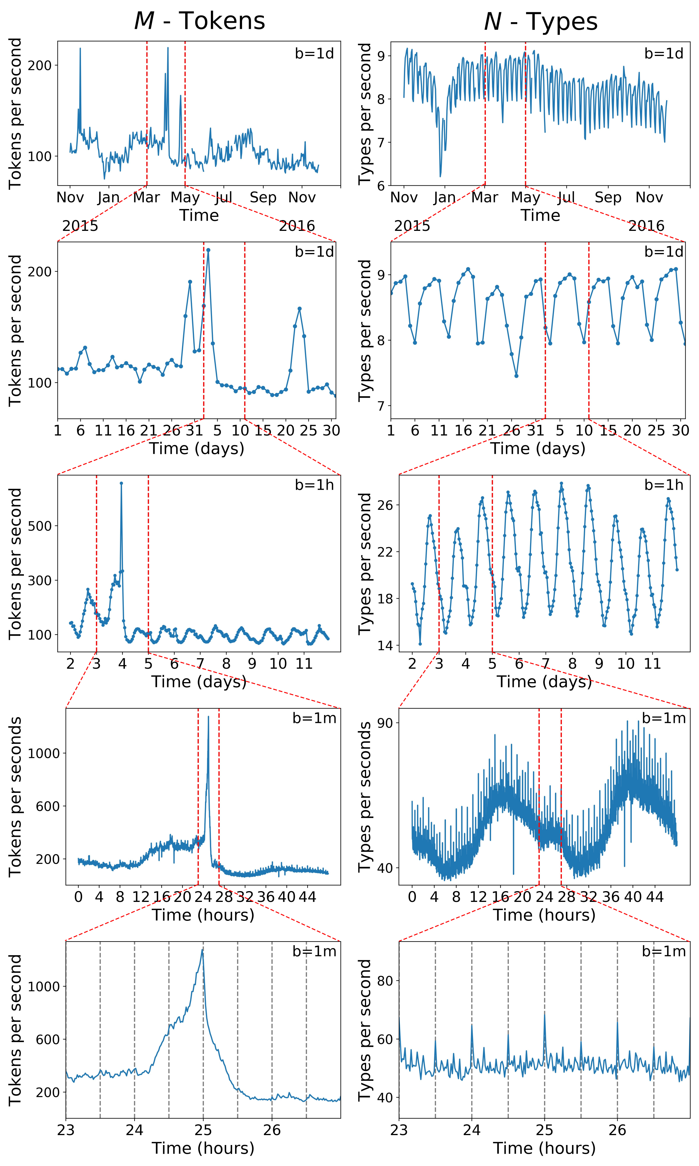
Figure 1: Time series of hashtag tokens $M(t)$ (left column) and types $N(t)$ (right column). Reported (y-axis) is the rate of usage ($N/b$ and $M/b$ with $b$ measured in seconds). Each panel corresponds to a magnification in the time scale (x-axis) of the panel immediately above it in the region indicated by vertical dashed (red) lines. In the two top panels the data was aggregated at different scales $b$: $b=1$ day for the two top panels, $b=1$ hour for the middle panels, and $b=1$ minute for the lower two panels footnote1 . Time corresponds to GMT.

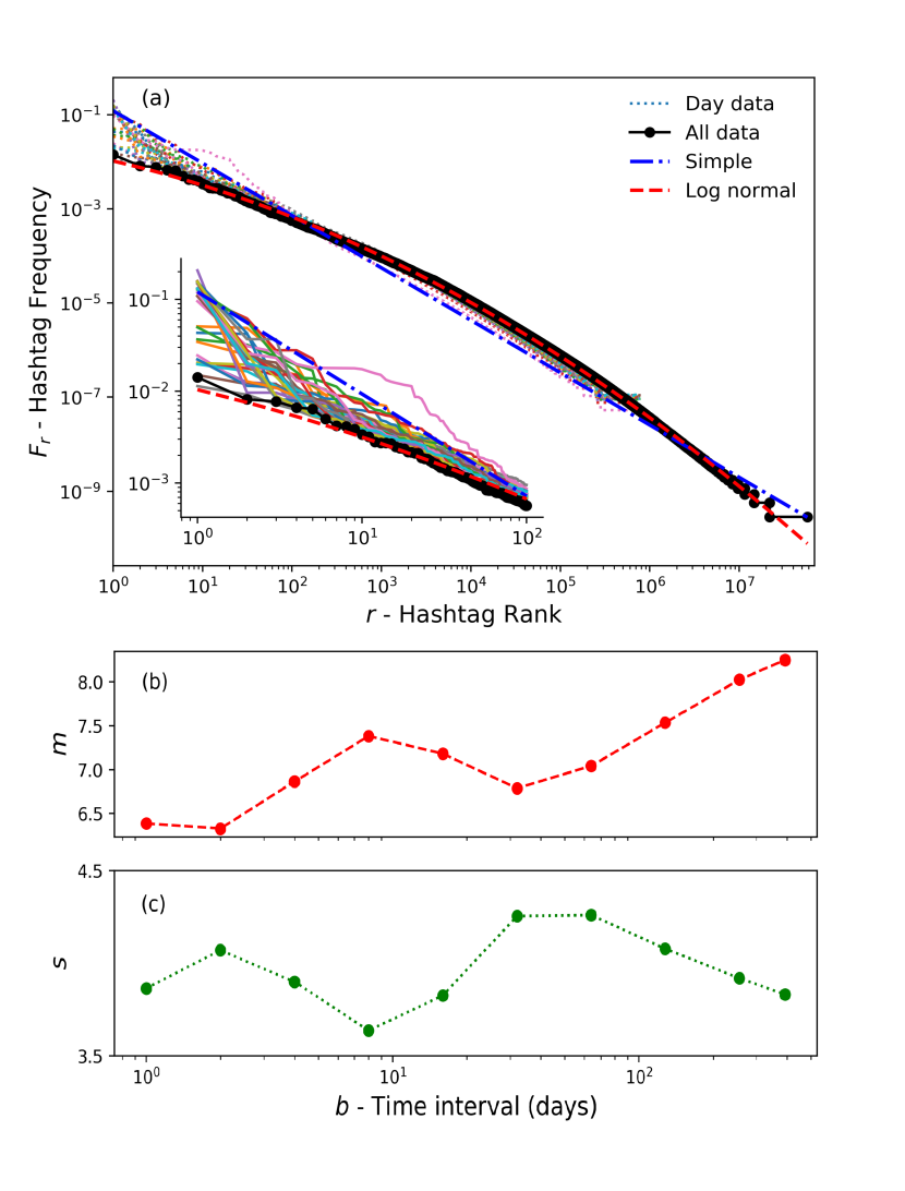
Figure 2: Fat-tailed distribution of hashtag frequencies. The solid (black) curve shows the frequency $F_{r}$ (y-axis) of the $r$-th (x-axis) most frequent hashtag in our complete database $b=392$ days. The thin (colored) lines show the results obtained for $30$ different cases with $b=1$ day. The inset shows a magnification for small $r$. In the main panel, the dotted line corresponds to Zipf’s law (1) with the maximum-likelihood parameter $\hat{\gamma}=1.13$ inferred from the data and the dashed (red) line correspond to the best generalized Zipf’s law given by Eq. (2) with estimated parameters $\hat{m}=8.25,\hat{s}=3.83$. The lower panels show how the parameters $\hat{m}$ and $\hat{s}$ vary with the size of the database $b$ used in the estimate, i.e., we used all hashtags in the time interval $[t,t+b]$ with $t$ fixed (the minimum) and varying $b$.

Our database consists of all hashtags used in a 10% sample of all tweets published between November 1st 2015 and November 30th 2016. For a given time interval $([t,t+b])$ around time t and of (bin) size $b$, we count how many hashtags were used in our database. Here it is important to distinguish between hashtag types (i.e., unique hashtags) and hashtag tokens (i.e., the repetitive usage of potentially the same hashtags). For instance, in our complete database ($b=392$ days) the hashtag type “#mtvstars” is the most frequently used hashtag (rank $r=1$), responsible for the appearance of $M_{r=1}=49M$ hashtag tokens. Next we have “#kca” with $M_{r=2}=28M$ and “#iheartawards” with $M_{r=3}=26M$. Overall, we have $N=57,876,308$ types and $M=\sum_{r=1}^{N}M_{r}=3,492,300,357$ tokens in our database. We denote $N(t)$ and $M(t)$ as the number of hashtag types and tokens, respectively, in an interval of size $b$ starting at time $t$ footnote1 .

Figure 1 shows how the number of hashtag tokens $M$ and types $N$ change in time $t$ at different time scales. The time series of tokens $M(t)$ shows a more noisy behaviour than the time series $N(t)$ of types: $M(t)$ shows pronounced bursts and spikes while $N(t)$ reflects more clearly the weekly and daily oscillations of Twitter usage. We see a weekly minimum in activity on a Sunday, while the daily maximum occurs around 1600 GMT. At short time scales, both time series have peaks at the first minute of each hour and each half hour, suggesting that a large number of pre-programmed tweets are being launched at regular patterns. The main peak in $M(t)$ highlighted in this figure is mostly due to the hashtag “#iheartawards” which was used during a music awards show that took place in the USA on the 3rd of April 2016 and has rank $r=3$ in our complete database.

III Zipf’s law

We are interested in the share of total hashtag tokens obtained by the different hashtag types, which can be interpreted as the success rate of individual memes in attracting the attention of users Tsur2012 . This possibility of the ‘rich-getting-richer’ element of hashtag use suggests that a fat-tailed distribution should be expected, because of the ubiquity of such a distribution type in data from natural and social systems Cunha2011 ; mitzenmacher2004 ; newman2005 . Possibly the best known example of such a distribution is Zipf’s law, which states that the frequency $F_{r}=M_{r}/M$ (i.e., the fraction of all tokens) of the $r$-th most frequent word (type) decays with $r$ as

$$F_{r}\sim r^{-\gamma},$$ (1)

with $\gamma\gtrapprox 1$.

In Fig. 2 we show a representation of the hashtag distribution. We observe that a similar distribution is observed for different time intervals, that the distribution spans many orders of magnitude – in agreement with the fat-tailed character of Eq. (1) –, and that the distribution shows a positive concavity (in the double-logarithmic plot) indicating a faster than Zipfian decay. All these observations have been reported for the frequency of words in a recent analysis of Zipf’s law in a large data set (Google n-grams) gerlach2013 and are consistent with previous analysis of hashtag frequencies Cunha2011 .

The observations above motivate us to consider whether generalizations of Zipf’s law proposed to describe word frequencies are also describing hashtag frequencies. We considered the distributions and methodology proposed in Ref. gerlach2013 to determine which of the eight parameterizations of $F_{r}$ best describes our hashtag data. Table 1 lists the different distributions, the best inferred parameters, and a measure of the agreement between data and the (best) distributions. The results show that the best generalized Zipf’s law is obtained by a log-normal fit of the rank distribution:

$$F_{r}=Cr^{-1}\text{exp}(-\frac{1}{2}(\text{ln}(r)-m)^{2}/s^{2})$$ (2)

where $C=C(m,s)$ is a normalization constant and $m,s$ are free parameters such that $m<s^{2}$. The restriction in the parameter choice is necessary to ensure that Eq. (2) is monotonically decaying in the integers $r$. This is necessary because, by construction, $F_{r}$ is monotonically decaying (a log-normal distribution in $F_{r}$ does not imply that the number of hashtag types with a given frequency $M_{i}/M$ is also log-normal). A further indication that the distribution 2 provides a good description of the data for different times $t$ is the fact that the estimated parameters $m$ and $s$ do not strongly depend on the size of the database $b$ (see lower panel of Fig. 2). This is a different finding from the one reported for natural language, where a double power-law distribution provided a better fit ferrericancho2001 ; gerlach2013 . Differently from the case of language, in the case of hashtags the double gamma distribution (with 3 free parameters) leads to a smaller likelihood $\mathcal{L}$ (or larger $-\log\mathcal{L}$) than the log-normal. Moreover, the parameters of the double gamma in the hashtag distributions differ from the case of language: while for language the first exponent was $\gamma=1$ (as originally proposed by Zipf), in the case of hashtags the first exponent is $\gamma\approx 0.8<1$. Altogether, in comparison to word frequencies, hashtags have a slower initial decay of $F_{r}$ (i.e., the top ranked hashtags have a more similar frequency) and a faster asymptotic decay of $F_{r}$ (which is faster than a power-law but slower than an exponential).

Model	$F_{r}\equiv F(r|\;\Omega)$	Parameter Estimates	$-\log\mathcal{L}/M$
Simple	$Cr^{-\gamma}$	$\gamma$ = 1.11	11.544
Shifted Power Law	$C(r+a)^{-\gamma}$	$\gamma$ = 1.25, $a$ = 119.8	11.205
Exponential cut off	$C\text{exp}(-ar)r^{-\gamma}$	$\gamma$ = 0.96, $a$ = 1.11	11.195
Naranan	$C\text{exp}(-a/r)r^{-\gamma}$	$\gamma$ = 1.16, $a$ = 5.0931	11.347
Weibull	$C\text{exp}(-ar^{-\gamma})r^{\gamma-1}$	$\gamma$ = -0.24, $a$ = 4.51	12.175
Log-normal	$Cr^{-1}\text{exp}(-\frac{1}{2}(\text{ln}(r)-m)^{2}/s^{2})$	$m$ = 8.25, $s$ = 3.83	11.075
Double Power Law	$C\begin{cases}r^{-1}&r\leq a\\ a^{\gamma-1}r^{-\gamma}&r>a\end{cases}$	$\gamma$ = 1.57, $a$ = 352288.8	11.186
Double Gamma	$C\begin{cases}r^{-\gamma_{1}}&r\leq a\\ a^{\gamma_{2}-\gamma_{1}}r^{-\gamma_{2}}&r>a\end{cases}$	$\gamma_{1}$ = 0.8083, $\gamma_{2}$ = 1.4079, $a$ = 18145.1	11.091

Table 1: Generalized Zipf’s law for hashtag frequencies. Different models for the rank-frequency distribution $F_{r}\equiv F(r|\Omega)$ were fitted to the empirical distribution $F_{r}$ using the maximum likelihood methods proposed in Ref. gerlach2013 . The parameters $\Omega$ that maximize the likelihood $\mathcal{L}$ are reported together with the negative log-likelihood per token $-\log\mathcal{L}/M$ (at the given parameters). The model with maximum likelihood (minimum $-\log\mathcal{L}$) is the log-normal model.

IV Heaps’ and Taylor’s laws

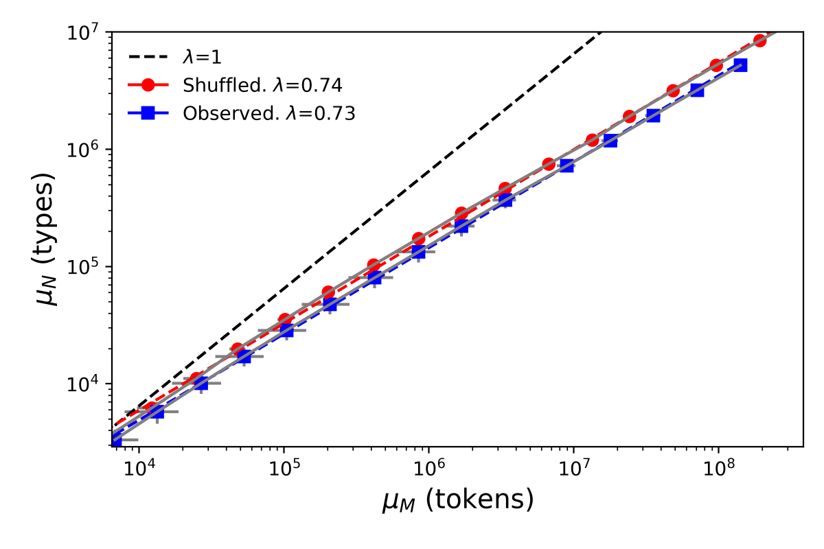
Figure 3: The expected number of types $\mu_{N}$ and tokens $\mu_{M}$ scale non-linearly as described by Heaps’ law (3). The hashtag data – $\blacksquare$ with (blue) line – was obtained using time intervals $b$ ranging from $b=1$ minute to $b=256$ days. The error bars correspond to $\sigma_{M}$ (x-axis) and $\sigma_{N}$ (y-axis). The results obtained after shuffling the temporal order of $M(t)$ and $N(t)$ obtained the scale of $b=1$ minute are shown as $\bullet$ with (red) line. The scaling exponents $\lambda$ indicated in the legend were obtained from a linear regression of the average results (dashed lines).

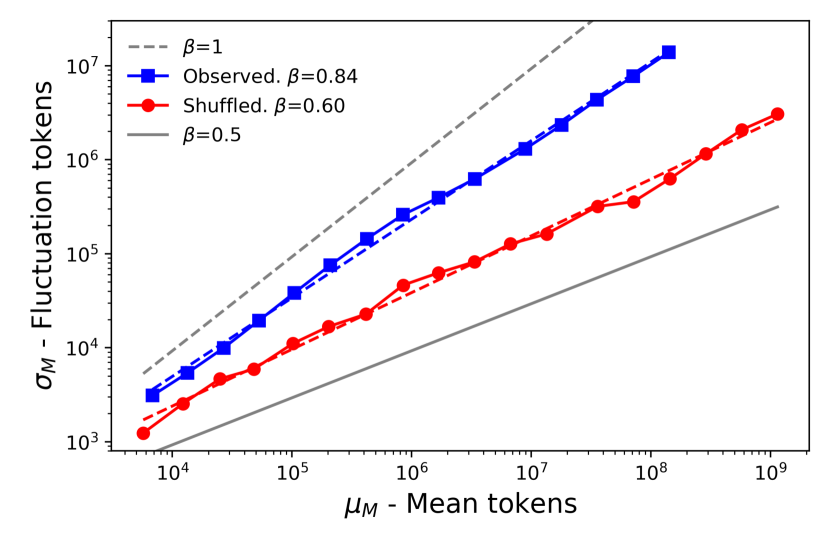
Figure 4: Fluctuations and average number of tokens scale non-linearly as described by Taylor’s law (6). The average $\mu_{M}$ (x-axis) and standard deviation $\sigma_{M}$ (y-axis) of the hashtag data – $\blacksquare$ with (blue) line – were obtained for intervals ranging from $b=1$ minute to $b=256$ days. The results obtained after shuffling the temporal order of $M(t)$ and $N(t)$ are shown as $\bullet$ with (red) line. The shuffling performed at the scales of $b=1$ minute, $b=1$ hour, and $b=1$ day all showed the same scaling with a different pre-factor. The plot shows a combined curve obtained after re-scaling the curves for $b=1$ hour and $b=1$ day by a constant factor so that they agree with the $b=1$ minute curve. The scaling exponents $\beta$ indicated in the legend were obtained by linear regression (dashed lines).

The Zipfian-type behaviour of hashtag frequencies motivates us to consider also other statistical laws proposed in quantitative linguistics ferrericancho2001 ; zanette2005 ; fontclos2013 ; gerlach2013 ; altmann2016 ; tanaka-ishii2019 . We start with Heaps’ law, which states that the number of types $N$ and tokens $M$ scale nonlinearly as

$$N\sim M^{\lambda},$$ (3)

where $\lambda<1$ and the symbol $\sim$ indicates that the ratio of the left and right sides tend to a constant for large $M$. To perform this analysis we compute $M(t)$ and $N(t)$ at different time intervals $[t,t+b]$, for different $t$’s and $b$’s as above. We then consider averages $\langle\ldots\rangle$ over all times $t$ for a fixed $b$ and compute the expected value and standard deviation of these quantities as

$$\mu_{M}=\langle M(t)\rangle,\sigma_{M}=\sqrt{\langle M^{2}(t)\rangle-\langle M(t)\rangle^{2}}$$ (4)

$$\mu_{N}=\langle N(t)\rangle,\sigma_{N}=\sqrt{\langle N^{2}(t)\rangle-\langle N(t)\rangle^{2}}.$$ (5)

By varying $b$ from minutes to months we effectively vary the size of the database over many orders of magnitude, allowing us to explore the scaling between these quantities.

In our case, Heaps’ law (3) is interpreted as the relation between how $\mu_{N}$ (the expected number of types $N$) scales with $\mu_{M}$ (the expected number of tokens $M$). The results in Fig. 3 reveal a striking scaling law over more than four decades, with an estimated exponent $\lambda\approx 0.73$. In this plot we also show the results obtained after shuffling the series at the scale of $b=1$ minute. We observe that $\mu_{N}$ is increased in the randomized data, reflecting the existing correlation between the hashtags used in neighbouring time intervals gerlach2014 . However, the same Heaps law scaling is observed for the shuffled data, in agreement with the previous demonstrations that Heaps’ law can be obtained from a random sampling of Zipf’s law gerlach2014 .

We now investigate how the fluctuations $\sigma$ scale with the mean $\mu$ as

$$\sigma\sim\mu^{\beta}.$$ (6)

Ref. reviewtaylor provides a review of this scaling, known as Taylor’s law, showing its appearance and significance in various complex systems. The exponent $\beta=1/2$ is obtained if we consider that the quantity of interest ($M$ in our case) is obtained as the sum of random quantities sampled independently from a distribution with a well-defined second moment. In our case, we can think that the values $M$ in a time interval $[t,t+b]$ is obtained as the sum of the number of hashtags at smaller scales. The case $\beta=1$ reflects the lack of mixing in the the terms being summed reviewtaylor ; gerlach2014 . Nontrivial values, $0.5<\beta<1$, are obtained in the presence of long-range correlations (in time $t$) or if the underlying distribution from which samples are taken does not have a second moment (large fluctuations of $M$ in small time intervals). In natural language, $\beta=1$ was observed for the case of word types $N$ gerlach2014 and $0.5<\beta<1$ was reported for the fluctuation of individual words tanaka-ishii2019

The results for our hashtag data set are reported in Fig. 4 and indicate that the exponent $\beta\approx 0.84$ is clearly within the range of non-trivial values (i.e., clearly different from $\beta=0.5$ and $\beta=1.0$). In order to clarify the origin of this non-trivial exponent we repeat the analysis after randomizing the time series $M(t)$. As expected, the exponent after the randomization $\beta_{R}\approx 0.6$ is smaller than the original exponent. The fact that this exponent is still larger than $1/2$ indicates that the origin of the non-trivial Taylor’s law in the hashtag frequencies is due to both long-range correlation in $M(t)$ and sampling from an underlying fat-tailed distribution (with diverging second moment). The latter point is consistent with the bursty behaviour of $N(t)$ reported in Fig. 1 above, and also with the results of Ref. domenico2019 .

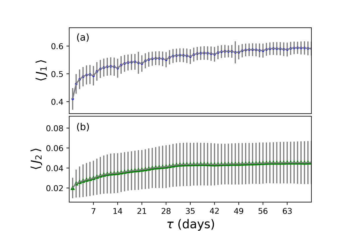
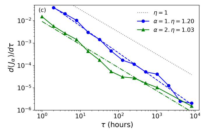
Figure 5: Dynamics of hashtags. Panels (a) and (b) show the distance $\langle J_{\alpha}\rangle$ (y-axis) between the hashtag usage separated by time $\tau$ (x-axis). The symbols (error bars) correspond to the average (standard deviation) $J_{\alpha}$ computed over all times $t$ for a fixed time separation $\tau$. The $\alpha$ entropy in Eq. (7) was used to compute $J_{\alpha}$ in Eq. (9) for $\alpha=1$ (a) and $\alpha=2$ (b). Panel (c) shows the derivative $d\langle J_{\alpha}\rangle/d\tau$ of the curves in panels (a) and (b), revealing a scaling law between $d\langle J_{\alpha}\rangle/d\tau$ and $\tau$ The maximum possible value of $J_{1}$ is $J_{1}=\sqrt{\ln 2}\approx 0.83$ gerlach2016 .

V hashtag Dynamics

	Words in Texts (English)	Hashtags in Twitter
Zipf-like decay of frequency $F_{r}$	Yes, faster than $r^{-1}$	Yes, faster than $r^{-1}$
Best generalized Zipf’s law	Double power law ferrericancho2001 ; gerlach2013 $\begin{cases}r^{-1}&r\leq a\\ a^{\gamma-1}r^{-\gamma}&r>a\end{cases}$	Log-normal $Cr^{-1}\text{exp}(-\frac{1}{2}(\text{ln}(r)-m)^{2}/s^{2})$
Heaps’ law $M\sim N^{\beta}$	$\beta\in[0.52,0.62]$ gerlach2013	$\beta=0.73$
Taylor’s law $\mu\sim\sigma^{\lambda}$	$\lambda=1$ gerlach2014	$\lambda=0.84$
Dynamics $J_{\alpha}$	Linear growth over centuries, constant $dJ/d\tau$  gerlach2016	Sub-linear growth over months, $dJ/d\tau\sim 1/\tau^{\eta}$

Table 2: Statistical laws for the frequency of hashtags in Twitter and for the frequency of words in texts.

So far we have concentrated on general statistical characterizations of hashtag frequencies that remain roughly invariant over time $t$, finding a Zipfian-like distribution and different scales between the total number of hashtag types $N$ and tokens $M$. Underlying these relationships there is a rich dynamical process of the usage $N_{i}(t)$ of individual hashtags. Our goal here is to quantify the extent into which, collectively, the frequency of all $M$ hashtags change over time. We use an information theoretic measure to quantify the similarity of two (normalized) frequency distributions, $F_{r}(t_{1})$ and $F_{r}(t_{2})$, following the approach used in Ref. gerlach2016 for language.

For each hashtag type $n=1,\ldots,N$ we define the frequency at time $t_{s}$ as $p_{n}=M_{n}(t_{s})/M(t_{s})$. We consider the frequencies $p_{n}$ to be an estimate of the probability of using this hashtag and $\bm{p}=(p_{1},p_{2},\ldots,p_{N})$ the probability distribution over all hashtags. The $\alpha$ entropy of $\bm{p}$ is defined as

$$H_{\alpha}(\bm{p})=\frac{1}{1-\alpha}\left(\sum_{i}p_{i}^{\alpha}-1\right)$$ (7)

and the similarity between two distributions, $\bm{p}$ and $\bm{q}$, can be quantified using the $\alpha$-generalized Jensen-Shannon divergence

$$D_{\alpha}(\bm{p},\bm{q})=H_{\alpha}\left(\frac{\bm{p}+\bm{q}}{2}\right)-\frac{1}{2}H_{\alpha}(\bm{p})-\frac{1}{2}H_{\alpha}(\bm{q}).$$ (8)

For $\alpha=1$ we recover the usual Shannon Entropy $H(\bm{p})=-\sum_{i}p_{i}\log p_{i}$ and Jensen-Shannon divergence, which can be viewed as a symmetrized Kullback-Leibler divergence. Finally, we quantify the similarity between distributions by taking the square root of the divergence

$$J_{\alpha}\equiv\sqrt{D_{\alpha}}.$$ (9)

As $J_{\alpha}$ has metric properties for $0\leq\alpha\leq 2$, it is a natural choice to measure distance. We use $\alpha=1$ and $\alpha=2$ to obtain different perspectives on the dynamics of hashtags: larger values of $\alpha$ give more weight to high-frequency hashtags gerlach2016 . Moreover, the statistical estimators of $J_{\alpha}$ converge very slowly with sample size $M$ for data with Zipfian frequency distribution gerlach2016 ; koplenig2019 and are better for $\alpha=2$ when compared to the usual $\alpha=1$.

The results obtained for our hashtag data are reported in Fig. 5 and show rich dynamics. The growth of $\langle J_{\alpha}\rangle$ with $\tau$ indicates that the measures $J_{\alpha}$ (9) are able to quantify the changes in hashtag frequencies we are interested in. Weekly oscillations are clearly visible in $J_{1}$ but not in $J_{2}$, indicating that there are a large number of hashtags that are not among the top ranked ones but are used repeatedly in the same day of the week (e.g., “#MondayMotivation”). The overall growth of $J_{\alpha}$ is slowing down with $\tau$ (i.e., the change in hashtag frequencies is larger for smaller $\tau$’s). Our main empirical finding is that this slow down follows an orderly pattern, described by the scaling law

$$d\langle J\rangle/d\tau\sim 1/\tau^{\eta},$$ (10)

with $\eta\gtrapprox 1$. This suggests that there is no characteristic time scale for the change of hashtag frequencies in Twitter but that instead it slows down in a self-similar fashion.

VI Conclusions

In summary, we provided a general statistical characterization of the frequency of hashtags on Twitter. We found that the frequency distribution follows a Zipfian pattern with a faster decay than a simple power-law. We found that this distribution is well described by the log-normal rank-frequency distribution (2). The type-token relationship shows a scaling law characteristic of Heaps’ law, with non-trivial large fluctuations around expected values that follow a fluctuation scaling relationship (Taylor’s law). These large fluctuations are due to the very noisy dynamics of hashtag tokens, that shows fat-tailed fluctuations and long-range temporal correlations. We also quantified the collective dynamics due to the change in the frequency $p_{i}$ of individual hashtags $i$ using a generalized Jensen-Shannon divergence. We found that the distance between hashtag distributions separated by time $\tau$ grows with $\tau$, showing weak oscillations (i.e., distributions at the same day of the week are more similar to each other) and that the velocity of the change decays with $\tau$, following a newly discovered scaling law, $1/\tau^{\eta}$ with $\eta\gtrapprox 1$.

A comparison of our findings to previous results for the frequency of words in large collections of texts is given in Tab. 2. It reveals striking similarities but also notable differences due to the different dynamics of hashtag and word frequencies. While in texts word tokens of the same word type cluster together, this happens in the middle of many high-frequency function words that permeate the texts with a more regular frequency. In contrast, the appearance of a (new) hashtag can trigger a large response of the usage of the same hashtag, leading to much wider fluctuations and correlations. In fact, the top-ranked word in English (“the”) remains the same over centuries, showing a frequency $F_{1}\approx 5\%$ that varies only slightly (between $4\%$ and $6\%$) over 200 years (in the Google n-gram database). In contrast, the most frequent hashtag not only varies from day to day but also the frequency of the top ranked hashtag can vary dramatically. For instance, on the first day of our data set (01-11-2015) the top ranked hashtag was “#pushawardskathniels” with a frequency of $4.3\%$, while the hashtag “#mtvstars” was ranked 143rd with a frequency of $0.05\%$. Two weeks later, the hashtags “#pushawardskathniels” and “#mtvstars” were ranked 10th and 1st respectively, with frequencies of $0.7\%$ and $10.9\%$.

A number of our statistical observations are similar to observations reported in isolation in earlier work, such as the burstiness of hashtags and high variability between hashtag volumes Tsur2012 , the appearance of fat-tailed distributions in the frequency of hashtags Cunha2011 , and the steady evolution of social media language with time GrieveELL2017 . With the combined statistical laws articulated here we hope to provide a framework for generative models to be compared with. Our findings provide statistical results that (modifications of) existing mechanistic models of social dynamics OliveiraChan ; bagrow2018 , language zanette2005 ; gerlach2013 , and Twitter gleeson2016 ; domenico2019 should reproduce. Next steps could be to verify in which extent previous models are able to reproduce our observations and to look in more detail at the nature of the hashtag evolution, e.g., to clarify whether certain types (sub-populations) of hashtags lead to different statistical features or whether the nature of hashtag usage changes more broadly at longer timescales.

Data Availability:

all data is available at https://doi.org/10.5281/zenodo.3673744

References

- (1) J. Hurlock and M.L. Wilson, “Searching Twitter: Separating the Tweet from the Chaff”, Proceedings of the Fifth International AAAI Conference on Weblogs and Social Media, (2011)
- (2) M. Zappavigna, “Searchable talk: the linguistic functions of hashtags”, Social Semiotics 25, 274 (2015)
- (3) M. Zappavigna, Searchable Talk: hashtags and Social Media Metadiscourse (Bloomsbury Academic, London, 2018)
- (4) J. P. Bagrow and L. Mitchell, ”The quoter model: A paradigmatic model of the social flow of written information”, Chaos 28, 075304 (2018).
- (5) M. E. J. Newman, ”Power Laws, Pareto Distributions and Zipf’s law”, Contemp. Phys.46, 323 (2005).
- (6) M. Mitzenmacher, ”A Brief History of Generative Models for Power Law and Log-normal Distributions”, Internet Math. 1, 226 (2004).
- (7) E. Cunha, G. Magno, G. Comarela, V. Giovanni, M.A. Gonçalves and F. Benevenuto, “Analyzing the Dynamic Evolution of hashtags on Twitter: A Language-Based Approach”, Proceedings of the Workshop on Languages in Social Media p58 (2011)
- (8) M. Naaman, H. Becker and L. Gravano, “Hip and trendy: Characterizing emerging trends on Twitter”, J. Am. Soc. Inform. Sci. Tech. 62, 902 (2011)
- (9) D. M. Beskow, S. Kumar and K.M. Carley, “The evolution of political memes: Detecting and characterizing internet memes with multi-modal deep learning”, Information Processing & Management 57, 102170 (2020)
- (10) D. M. Romero, B. Meeder and J. Kleinberg, “Differences in the Mechanics of Information Diffusion across Topics: Idioms, Political hashtags, and Complex Contagion on Twitter”, Proceedings of the 20th International Conference on World Wide Web p695 (2011)
- (11) J. P. Gleeson, K. P. O’Sullivan, R. A. Baños, and Y. Moreno, Effects of Network Structure, Competition and Memory Time on Social Spreading Phenomena, Phys. Rev. X. 6, 021019 (2016)
- (12) M. De Domenico and E. G. Altmann ”Unraveling the Origin of Social Bursts in Collective Attention” arXiv:1903.06588 (2019)
- (13) L. Weng, A. Flammini, A. Vespignani, and F. Menczer. Competition among memes in a world with limited attention. Scientific Reports 2 335 (2012).
- (14) K. Lerman, R. Ghosh, and T. Surachawala. Social contagion: An empirical study of information spread on Digg and Twitter follower graphs. arXiv preprint arXiv:1202.3162 (2012).
- (15) N., Daniele, and C. Castellano. Analytical study of quality-biased competition dynamics for memes in social media. EPL (Europhysics Letters) 122, 28002 (2018).
- (16) M. Tremayne, “Anatomy of Protest in the Digital Era: A Network Analysis of Twitter and Occupy Wall Street”, Social Movement Studies 13, 110 (2014)
- (17) K. G. Kapanova and S. Fidanova, “Generalized Nets: A New Approach to Model a hashtag Linguistic Network on Twitter” in Advanced Computing in Industrial Mathematics: 12th Annual Meeting of the Bulgarian Section of SIAM December 20-22, 2017, Sofia, Bulgaria Revised Selected Papers, edited by K. Georgiev, M. Todorov and I. Georgiev (Springer International Publishing, 2019), p211.
- (18) H. Bingol. Fame emerges as a result of small memory. Physical Review E 77, 036118 (2008).
- (19) J. Ratkiewicz, S. Fortunato, A. Flammini, F. Menczer, and A. Vespignani. Characterizing and modeling the dynamics of online popularity. Physical review letters 105 158701 (2010).
- (20) D. F. M. Oliveira, K. S. Chan. The effects of trust and influence on the spreading of low and high quality information. Physica A: Statistical Mechanics and its Applications 525, 657-663 (2019)
- (21) R. Ferrer-i-Cancho and R.V. Solé, ”Two regimes in the frequency of words and the origins of complex Lexicons: Zipf’s law revisited”, Journal of Quantitative Linguistics 8, 165 (2001).
- (22) D. Zanette and M. Montemurro, ”Dynamics of Text Generation with Realistic Zipf’s Distribution”, Journal of Quantitative Lingusitics 12, 29 (2005).
- (23) M. Gerlach and E. G. Altmann, ”Stochastic model for the vocabulary growth in natural languages”, Phys. Rev. X 3, 021006 (2013)
- (24) F. Font-Clos, G. Boleda, and A. Corral, ”A scaling law beyond Zipf’s law and its relation to Heaps’law”, New Journal of Physics 15, 093033 (2013).
- (25) M. Gerlach and E. G. Altmann, ”Scaling laws and fluctuations in the statistics of word frequencies”, New J. Physics 15, 113010 (2014)
- (26) E. G. Altmann and M. Gerlach, ”Statistical laws in linguistics”, in Creativity and niversality in language, 7-26, Lecture notes in Morphogenesis, Springer, (2016)
- (27) K. Tanaka-Ishii1 and Tatsuru Kobayashi, ”Taylor’s law for linguistic sequences and random walk models”, J. Phys. Commun. 3 089401 (2019)
- (28) M. Gerlach, F. Font-Clos, and E. G. Altmann, ”On the similarity of symbol-frequency distributions with heavy tails”, Phys. Rev. X 6, 021009 (2016).
- (29) A. Koplenig, S. Wolfer, and C. Müller-Spitzer, ”Studying Lexical Dynamics and Language Change via Generalized Entropies: The Problem of Sample Size”, Entropy 21, 464 (2019).
- (30) O. Tsur and A. Rappoport, “What’s in a hashtag? Content Based Prediction of the Spread of Ideas in Microblogging Communities”, Proceedings of the Fifth ACM International Conference on Web Search and Data Mining, p643 (2012).
- (31) Z. Eisler, I. Bartos, and J. Kertész. Fluctuation scaling in complex systems: Taylor’s law and beyond. Advances in Physics 57 89-142 (2008).
- (32) J. Grieve, A. Nini and D. Guo, “Analyzing lexical emergence in Modern American English online”, English Language and Linguistics 21, 99 (2017).
- (33) An important difference between and is that is simply the sum of of sub-intervals (of smaller size ) while for this is not the case because we are interested in unique hashtags. This leads to a sub-linear relationship between types and tokens, which is investigated below in the context of Heaps’ law.