theoremdummy \aliascntresetthetheorem \newaliascntpropositiondummy \aliascntresettheproposition \newaliascntcorollarydummy \aliascntresetthecorollary \newaliascntlemmadummy \aliascntresetthelemma \newaliascntdefinitiondummy \aliascntresetthedefinition \newaliascntsublemmadummy \aliascntresetthesublemma \newaliascntclaimdummy \aliascntresettheclaim \newaliascntremarkdummy \aliascntresettheremark \newaliascntfactdummy \aliascntresetthefact \newaliascntconjecturedummy \aliascntresettheconjecture \newaliascntquestiondummy \aliascntresetthequestion \newaliascntobservationdummy \aliascntresettheobservation \newaliascntproblemdummy \aliascntresettheproblem \newaliascntnotedummy \aliascntresetthenote
-apices of minor-closed graph classes. II. Parameterized algorithms††thanks: A conference version of this paper appeared in the Proceedings of the 47th International Colloquium on Automata, Languages and Programming (ICALP), volume 168 of LIPICs, pages 95:1–95:20, 2020.
Abstract
Let be a minor-closed graph class. We say that a graph is a -apex of if contains a set of at most vertices such that belongs to . We denote by the set of all graphs that are -apices of In the first paper of this series we obtained upper bounds on the size of the graphs in the minor-obstruction set of , i.e., the minor-minimal set of graphs not belonging to In this article we provide an algorithm that, given a graph on vertices, runs in time and either returns a set certifying that , or reports that . Here is a polynomial function whose degree depends on the maximum size of a minor-obstruction of In the special case where excludes some apex graph as a minor, we give an alternative algorithm running in -time.
Keywords: graph minors; parameterized algorithms; graph modification problems; irrelevant vertex technique; Flat Wall Theorem.
1 Introduction
Graph modification problems are fundamental in algorithmic graph theory. Typically, such a problem is determined by a graph class and some prespecified set of local modifications, such as vertex/edge removal or edge addition/contraction or combinations of them, and the question is, given a graph and an integer whether it is possible to transform to a graph in by applying modification operations from A plethora of graph problems can be formulated for different instantiations of and Applications span diverse topics such as computational biology, computer vision, machine learning, networking, and sociology [FominSM15grap]. As reported by Roded Sharan in [Sharan02grap], already in 1979 Garey and Johnson mentioned 18 different types of modification problems [GareyJ79comp, Section A1.2]. For more on graph modification problems, see [FominSM15grap, BodlaenderHL14grap] as well as the running survey in [CrespelleDFG13asur]. In this paper we focus our attention on the vertex deletion operation. We say that a graph is a -apex of a graph class if there is a set of size at most such that the removal of from results in a graph in In other words, we consider the following meta-problem.
Vertex Deletion to
Input: A graph and a non-negative integer
Objective: Find, if it exists, a set certifying that is -apex of
To illustrate the expressive power of Vertex Deletion to , if is the class of edgeless (resp. acyclic, planar, bipartite, (proper) interval, chordal) graphs, we obtain the Vertex Cover (resp. Feedback Vertex Set, Vertex Planarization, Odd Cycle Transversal, (proper) Interval Vertex Deletion, Chordal Vertex Deletion) problem.
By the classical result of Lewis and Yannakakis [LewisY80then], Vertex Deletion to is NP-hard for every non-trivial graph class To circumvent its intractability, we study it from the parameterized complexity point of view and we parameterize it by the number of vertex deletions. In this setting, the most desirable behavior is the existence of an algorithm running in time where is a computable function depending only on Such an algorithm is called fixed-parameter tractable, or FPT-algorithm for short, and a parameterized problem admitting an FPT-algorithm is said to belong to the parameterized complexity class FPT. Also, the function is called parametric dependence of the corresponding FPT-algorithm, and the challenge is to design FPT-algorithms with small parametric dependencies [CyganFKLMPPS15para, DowneyF13fund, FlumG06para, Niedermeier06invi].
Unfortunately, we cannot hope for the existence of FPT-algorithms for every graph class Indeed, the problem is W-hard111Implying that an FPT-algorithm would result in an unexpected complexity collapse; see [DowneyF13fund]. for some classes that are closed under induced subgraphs [Lokshtanov08whee] or, even worse, NP-hard, for for every class whose recognition problem is NP-hard, such as some classes closed under subgraphs or induced subgraphs (for instance 3-colorable graphs), edge contractions [BrouwerV87cont], or induced minors [FellowsKMP95thec].
On the positive side, a very relevant subset of classes of graphs does allow for FPT-algorithms. These are classes that are closed under minors222A graph is a minor of a graph if it can be obtained from a subgraph of by contracting edges, see Subsection 2.2 for the formal definitions., or minor-closed. To see this, we define as the class of the -apices of i.e., the yes-instances of Vertex Deletion to , and observe that if is minor-closed then the same holds for for every This, in turn, implies that for every can be characterized by a set of minor-minimal graphs that are not in ; we call these graphs the obstructions of and we know that they are finite because of the Robertson and Seymour’s theorem [RobertsonS04XX]. In other words, we know that the size of the obstruction set of is bounded by some function of Then one can decide whether a graph belongs to by checking whether excludes all members of the obstruction set of and this can be checked by using the FPT-algorithm in [RobertsonS95XIII] (see also [FellowsL88nonc]).
As the Robertson and Seymour’s theorem [RobertsonS04XX] does not construct the aforementioned argument is not constructive, i.e., it is not able to construct the claimed FPT-algorithm. An important step towards the constructibility of such an FPT-algorithm was done by Adler et al. [AdlerGK08comp], who proved that is effectively computable. In the first paper of this series [SauST21kapiI] we give an explicit upper bound on the size of the graphs in namely we prove that every graph in has size bounded by an exponential tower of height four of a polynomial function in whose degree depends on the size of the minor-obstructions of The focus of the current paper is on the parametric dependence of FPT-algorithms to solve the Vertex Deletion to problem, i.e., for recognizing the class .
The task of specifying (or even optimizing) this parametric dependence for different instantiations of occupied a considerable part of research in parameterized algorithms. The most general result in this direction states that, for every there is some contant such that if the graphs in have treewidth at most then Vertex Deletion to admits an FPT-algorithm that runs in time [FominLMS12plan, KimLPRRSS16line]. Reducing the constant in this running time has attracted research on particular problems such as Vertex Cover[ChenKX10impr] (with ), Feedback Vertex Set [KociumakaP14fast] (with ), Apex-Pseudoforest [BodlaenderOO18afas] (with ), Pathwidth 1 Vertex Deletion (with )[CyganPPW12anim], or Pumpkin Vertex Deletion [JoretPSST14hitt]. The first step towards a parameterized algorithm for Vertex Deletion to for cases where has unbounded treewidth was done in [MarxS07obta] and later in [Kawarabayashi09plan] for the Vertex Planarization problem, and the best parameterized dependence for this problem is achieved by Jansen et al. [JansenLS14anea]. These results were later extended by Kociumaka and Marcin Pilipczuk [KociumakaP19dele], who proved that if is the class of graphs of Euler genus at most then Vertex Deletion to admits a -time333Given a tuple and two functions we write in order to denote that there exists a computable function such that algorithm.
Our results.
In this paper we give an explicit FPT-algorithm for Vertex Deletion to for every fixed minor-closed graph class In particular, our main results are the following.
Theorem \thetheorem.
If is a minor-closed graph class, then Vertex Deletion to admits an algorithm running in time for some polynomial poly whose degree depends on
We say that a graph is an apex graph if it is a 1-apex of the class of planar graphs.
Theorem \thetheorem.
If is a minor-closed graph class excluding some apex graph, then Vertex Deletion to admits an algorithm running in time for some polynomial poly whose degree depends on
Our techniques.
We provide here just a very succinct enumeration of the techniques that we use in order to achieve Section 1 and Section 1; a more detailed description with the corresponding definitions is provided, along with the algorithms, in the next sections.
Our starting point to prove Section 1 is to use the standard iterative compression technique of Reed et al. [ReedSV04find] (Subsection 5.2). This allows us to assume that we have at hand a slightly too large set such that We run the algorithm of Subsection 3.3 from [SauST21amor] that (since ) either concludes that the treewidth of is polynomially bounded by or finds a large flat wall together with an apex set In the first case, we use the main algorithmic result of Baste et al. [BasteST20acom] (Subsection 2.2) to solve the problem parameterized by treewidth, achieving the claimed running time. Subsection 3.3 is an improved version of the original “Flat Wall Theorem” of Robertson and Seymour [RobertsonS95XIII], whose proof is based on the recent results of Kawarabayashi et al. [KawarabayashiTW18anew], which we state using the framework that we recently introduced in [SauST21amor]. This framework is presented in Section 3 and provides the formal definitions of a series of combinatorial concepts such as paintings and renditions (Subsection 3.2), flatness pairs and tilts (Subsection 3.3), as well as a notion of wall homogeneity (Subsection 3.4) alternative to the one given in [RobertsonS95XIII]. All these concepts are extensively used in our proofs, as well as in those in the first article of this series [SauST21kapiI].
Once we have the large flat wall and the apex set , we see how many vertices of have enough neighbors in the “interior” of . Two possible scenarios may occur. If the “interior” of has enough neighbors in the set we apply a combinatorial result of [SauST21kapiI] (Subsection 4.2), based on the notion of canonical partition of a wall, that guarantees that every possible solution should intersect and we can branch on it.
On the other hand, if the interior of has few neighbors in , we find in a packing of an appropriate number of pairwise disjoint large enough subwalls (Subsection 4.2) and we find a subwall whose interior has few (a function not depending on ) neighbors in . We then argue that we can define from it a flat wall in which we can apply the irrelevant vertex technique of Robertson and Seymour [RobertsonS95XIII] (Subsection 4.1). We stress that this flat subwall is not precisely a subwall of but a tiny “tilt” of a subwall of a concept introduced in [SauST21amor] that is necessary for our proofs. In order to apply the irrelevant vertex technique, the main combinatorial tool is Subsection 4.1, which as been proved in [SauST21kapiI] and that is an enhancement of a result of Baste et al. [BasteST20acom], as we discuss in Subsection 4.1.
In order to achieve the improved running time claimed in Section 1, we do not use iterative compression. Instead, we directly invoke LABEL:label_improvements, which is a variation of [SauST21amor, Lemma 11] and whose proof uses [PerkovicR00anim, AlthausZ19opti, KawarabayashiK20line, AdlerDFST11fast], that either reports that we have a no-instance, or concludes that the treewidth of is polynomially bounded by or finds a large wall in If the treewidth is small, we proceed as above. If a large wall is found, we apply Subsection 3.3 and we now distinguish two cases. If a large flat wall is found, we find an irrelevant vertex using again Subsection 4.1. Otherwise, inspired by an idea of Marx and Schlotter [MarxS07obta], we exploit the fact that excludes an apex graph, and we use flow techniques to either find a vertex that should belong to the solution, or to conclude that we are dealing with a no-instance.
Organization of the paper.
In Section 2 we give some basic definitions and preliminary results. In Section 3 we introduce flat walls along with all the concepts and results around the Flat Wall Theorem, using the framework of [SauST21amor]. In Section 4 we present several algorithmic and combinatorial results that will be used in the algorithms, when finding an irrelevant vertex or when applying the branching step. In Section 5 and LABEL:label_demonstrieren we present the main algorithms claimed in Section 1 and Section 1, respectively. In LABEL:label_ressentiment we explain how to modify our algorithms so to deal with a series of variants of the Vertex Deletion to problem. We conclude in LABEL:label_grundgesetzen with some directions for further research.
2 Definitions and preliminary results
Our first step is to restate the problem in a more convenient way. We next give some basic definitions and preliminary results.
2.1 Restating the problem
Let be a finite non-empty collection of non-empty graphs. We use to denote that some graph in is a minor of
Given a graph class its minor obstruction set is defined as the set of all minor-minimal graphs that are not in , and is denoted by Given a finite non-empty collection of non-empty graphs we denote by as the set containing every graph that excludes all graphs in as minors.
Let be a minor-closed graph class and be its obstruction set. Clearly, Vertex Deletion to is the same problem as asking, given a graph and some for a vertex set of at most vertices such that Following the terminology of [BasteST20hittI, BasteST20hittII, BasteST20hittIII, BasteST20acom, FominLPSZ20hitt, FominLMS12plan, KimLPRRSS16line, KimST18data], we call this problem -M-Deletion.
Some conventions.
In what follows we always denote by the set of the instantiation of Vertex Deletion to that we consider. Notice that, given a graph and an integer is a yes-instance of -M-Deletion if and only if Given a graph we define its apex number to be the smallest integer for which is an -apex of the class of planar graphs. Also, we define the detail of denoted by to be the maximum among and We define three constants depending on that will be used throughout the paper whenever we consider such a collection We define as the minimum apex number of a graph in we set and we set Unless stated otherwise, we denote by and the number of vertices and edges, respectively, of the graph under consideration. We can always assume that has edges, otherwise we can directly conclude that is a no-instance (for this, use the fact that graphs excluding some graph as a minor are sparse [Kostochka82lowe, Thomason01thee]).
2.2 Preliminaries
Sets and integers.
We denote by the set of non-negative integers. Given two integers and the set contains every integer such that For an integer we set and Given a non-negative integer we denote by the minimum odd number that is not smaller than For a set we denote by the set of all subsets of and, given an integer we denote by the set of all subsets of of size and by the set of all subsets of of size at most If is a collection of objects where the operation is defined, then we denote
Basic concepts on graphs.
All graphs considered in this paper are undirected, finite, and without loops or multiple edges. We use standard graph-theoretic notation and we refer the reader to [Diestel10grap] for any undefined terminology. Let be a graph. We say that a pair is a separation of if and there is no edge in between and Given a vertex we denote by the set of vertices of that are adjacent to in A vertex is isolated if For we set and use the shortcut to denote Given a vertex of degree two with neighbors and we define the dissolution of to be the operation of deleting and, if and are not adjacent, adding the edge Given two graphs we say that is a dissolution of if can be obtained from after dissolving vertices of Given an edge we define the subdivision of to be the operation of deleting adding a new vertex and making it adjacent to and Given two graphs and we say that is a subdivision of if can be obtained from after subdividing edges of
Treewidth.
A tree decomposition of a graph is a pair where is a tree and such that
-
•
-
•
for every edge of there is a such that contains both endpoints of and
-
•
for every the subgraph of induced by is connected.
The width of is equal to and the treewidth of , denoted by , is the minimum width over all tree decompositions of
To compute a tree decomposition of a graph of bounded treewidth, in the proof of LABEL:label_improvements in LABEL:label_demonstrieren we will use the single-exponential -approximation algorithm for treewidth of Bodlaender et al. [BodlaenderDDFLP16ackn, Theorem VI].
Proposition \theproposition.
There is an algorithm that, given an graph and an integer outputs either a report that or a tree decomposition of of width at most Moreover, this algorithm runs in -time.
Contractions and minors.
The contraction of an edge of a simple graph results in a simple graph obtained from by adding a new vertex adjacent to all the vertices in the set A graph is a minor of a graph denoted by if can be obtained from by a sequence of vertex removals, edge removals, and edge contractions. If only edge contractions are allowed, we say that is a contraction of Given two graphs and if is a minor of then for every vertex there is a set of vertices in that are the endpoints of the edges of contracted towards creating We call this set model of in Recall that, given a finite collection of graphs and a graph we use notation to denote that some graph in is a minor of
We present here the main result of Baste et al. [BasteST20acom], which we will use in order to solve -M-Deletion on instances of treewidth bounded by an appropriate function of .
Proposition \theproposition.
Let be a finite collection of graphs. There exists an algorithm that, given a triple where is a graph of treewidth at most and is a non-negative integer, it outputs, if it exists, a vertex set of of size at most such that Moreover, this algorithm runs in -time.
3 Flat walls
In this section we deal with flat walls, using the framework of [SauST21amor]. More precisely, in Subsection 3.1, we introduce walls and several notions concerning them. In Subsection 3.2, we provide the definitions of a rendition and a painting. Using the above notions, in Subsection 3.3, we define flat walls and provide some results about them, including the Flat Wall Theorem (namely, the version proved by Kawarabayashi et al. [KawarabayashiTW18anew]) and its algorithmic version restated in the “more accurate” framework of [SauST21amor]. Finally, in Subsection 3.4, we present the notion of homogeneity and an algorithm from [SauST21amor] that allows us to detect a homogenous flat wall “inside” a given flat wall of “big enough” height. We note that the definitions of this section can also be found in [SauST21amor, SauST21kapiI].
3.1 Walls and subwalls
We start with some basic definitions about walls.
Walls.
Let The -grid is the graph whose vertex set is and two vertices and are adjacent if and only if An elementary -wall, for some odd integer is the graph obtained from a -grid with vertices after the removal of the “vertical” edges for odd and then the removal of all vertices of degree one. Notice that, as an elementary -wall is a planar graph that has a unique (up to topological isomorphism) embedding in the plane such that all its finite faces are incident to exactly six edges. The perimeter of an elementary -wall is the cycle bounding its infinite face, while the cycles bounding its finite faces are called bricks. Also, the vertices in the perimeter of an elementary -wall that have degree two are called pegs, while the vertices are called corners (notice that the corners are also pegs).
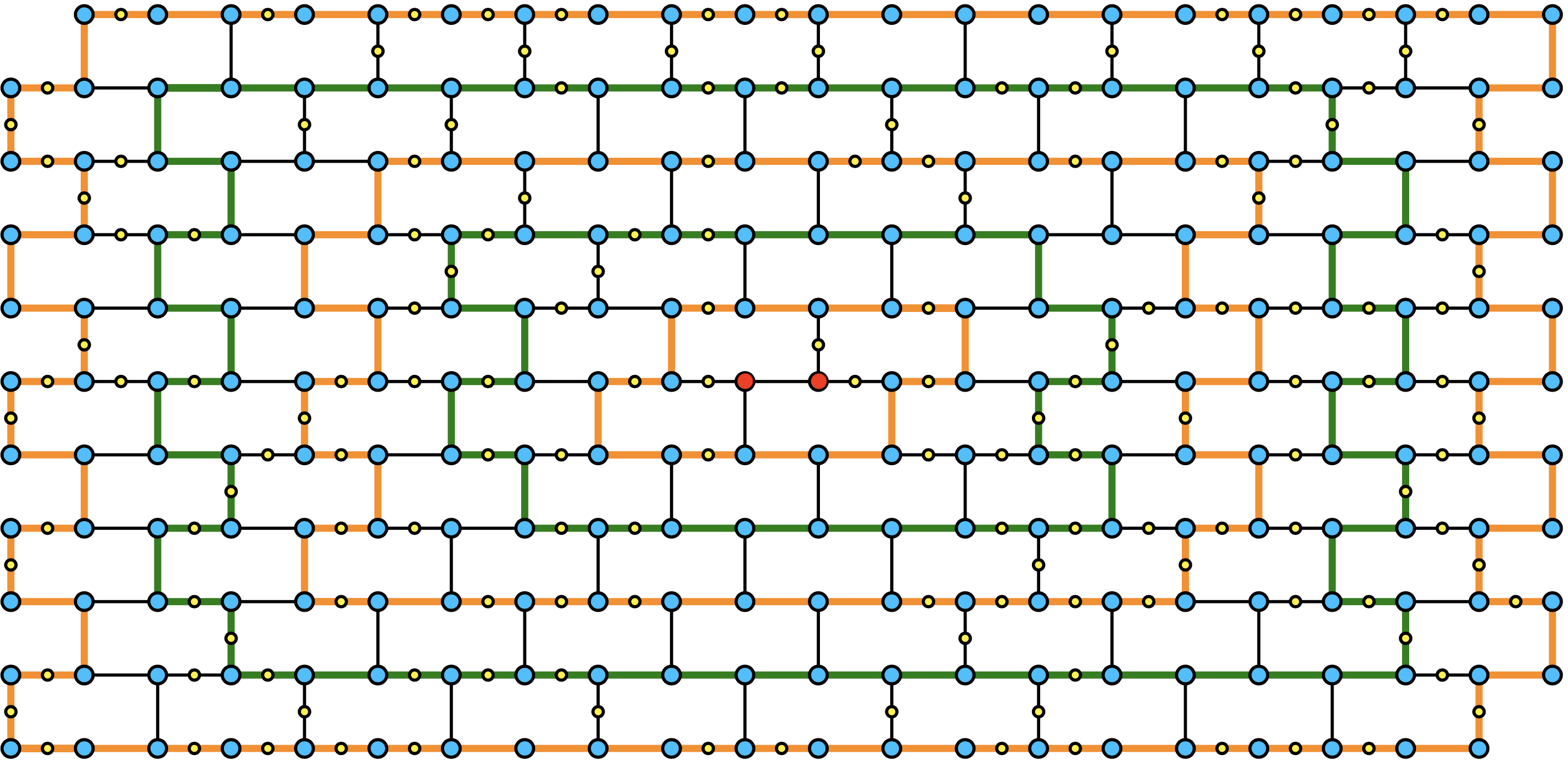
An -wall is any graph obtained from an elementary -wall after subdividing edges (see Figure 1). A graph is a wall if it is an -wall for some odd and we refer to as the height of Given a graph a wall of is a subgraph of that is a wall. We insist that, for every -wall, the number is always odd.
We call the vertices of degree three of a wall 3-branch vertices. A cycle of is a brick (resp. the perimeter) of if its 3-branch vertices are the vertices of a brick (resp. the perimeter) of We denote by the set of all cycles of We use in order to denote the perimeter of the wall A brick of is internal if it is disjoint from
Subwalls.
Given an elementary -wall some odd and the -th vertical path of is the one whose vertices, in order of appearance, are Also, given some the -th horizontal path of is the one whose vertices, in order of appearance, are
A vertical (resp. horizontal) path of an -wall is one that is a subdivision of a vertical (resp. horizontal) path of Notice that the perimeter of an -wall is uniquely defined regardless of the choice of the elementary -wall A subwall of is any subgraph of that is an -wall, with and such the vertical (resp. horizontal) paths of are subpaths of the vertical (resp. horizontal) paths of
Layers.
The layers of an -wall are recursively defined as follows. The first layer of is its perimeter. For the -th layer of is the -th layer of the subwall obtained from after removing from its perimeter and removing recursively all occurring vertices of degree one. We refer to the -th layer as the inner layer of The central vertices of an -wall are its two branch vertices that do not belong to any of its layers. See Figure 1 for an illustration of the notions defined above.
Central walls.
Given an -wall and an odd where we define the central -subwall of denoted by to be the -wall obtained from after removing its first layers and all occurring vertices of degree one.
Tilts.
The interior of a wall is the graph obtained from if we remove from it all edges of and all vertices of that have degree two in Given two walls and of a graph we say that is a tilt of if and have identical interiors.
The following result is derived from [AdlerDFST11fast]. We will use it in the improved algorithm of Section 1 in LABEL:label_demonstrieren, in order to find a wall in a graph of bounded treewidth, given a tree decomposition of it.
Proposition \theproposition.
There is an algorithm that, given a graph on edges, a graph on edges without isolated vertices, and a tree decomposition of of width at most it outputs, if it exists, a minor of isomorphic to Moreover, this algorithm runs in -time.
3.2 Paintings and renditions
In this subsection we present the notions of renditions and paintings, originating in the work of Robertson and Seymour [RobertsonS95XIII]. The definitions presented here were introduced by Kawarabayashi et al. [KawarabayashiTW18anew] (see also [BasteST20acom, SauST21amor]).
Paintings.
A closed (resp. open) disk is a set homeomorphic to the set (resp. ). Let be a closed disk. Given a subset of we denote its closure by and its boundary by A -painting is a pair where
-
•
is a finite set of points of
-
•
and
-
•
has finitely many arcwise-connected components, called cells, where, for every cell
-
the closure of is a closed disk and
-
where
-
We use the notation and denote the set of cells of by For convenience, we may assume that each cell of is an open disk of
Notice that, given a -painting the pair is a hypergraph whose hyperedges have cardinality at most three and can be seen as a plane embedding of this hypergraph in
Renditions.
Let be a graph and let be a cyclic permutation of a subset of that we denote by By an -rendition of we mean a triple where
-
(a)
is a -painting for some closed disk
-
(b)
is an injection, and
-
(c)
assigns to each cell a subgraph of such that
-
(1)
-
(2)
for distinct and are edge-disjoint,
-
(3)
for every cell
-
(4)
for every cell and
-
(5)
such that the points in appear in in the same ordering as their images, via in
-
(1)
3.3 Flatness pairs
In this subsection we define the notion of a flat wall. The definitions given in this subsection are originating in [SauST21amor]. We refer the reader to that paper for a more detailed exposition of these definitions and the reasons for which we introduced them. We use the more accurate framework of [SauST21amor] concerning flat walls, instead of that of [KawarabayashiTW18anew], in order to be able to use tools that are developed in [SauST21amor] and [SauST21kapiI] and will be useful in future applications as well.
Flat walls.
Let be a graph and let be an -wall of for some odd integer We say that a pair is a choice of pegs and corners for if is the subdivision of an elementary -wall where and are the pegs and the corners of respectively (clearly, ). To get more intuition, notice that a wall can occur in several ways from the elementary wall depending on the way the vertices in the perimeter of are subdivided. Each of them gives a different selection of pegs and corners of
We say that is a flat -wall of if there is a separation of and a choice of pegs and corners for such that:
-
•
-
•
and
-
•
if is the cyclic ordering of the vertices as they appear in then there exists an -rendition of
We say that is a flat wall of if it is a flat -wall for some odd integer
Flatness pairs.
Given the above, we say that the choice of the 7-tuple certifies that is a flat wall of . We call the pair a flatness pair of and define the height of the pair to be the height of We use the term cell of in order to refer to the cells of
We call the graph the -compass of in denoted by We can assume that is connected, updating by removing from the vertices of all the connected components of except of the one that contains and including them in ( can also be easily modified according to the removal of the aforementioned vertices from ). We define the flaps of the wall in as Given a flap we define its base as A cell of is untidy if contains a vertex of such that two of the edges of that are incident to are edges of Notice that if is untidy then A cell of is tidy if it is not untidy.
Cell classification.
Given a cycle of we say that is -normal if it is not a subgraph of a flap Given an -normal cycle of we call a cell of -perimetric if contains some edge of Notice that if is -perimetric, then contains two points such that and are vertices of where one, say of the two -subpaths of is a subgraph of and the other, denoted by -subpath contains at most one internal vertex of which should be the (unique) vertex in We pick a -arc in such that if and only if contains the vertex as an internal vertex.
We consider the circle and we denote by the closed disk bounded by that is contained in A cell of is called -internal if and is called -external if Notice that the cells of are partitioned into -internal, -perimetric, and -external cells.
Let be a tidy -perimetric cell of where Notice that has two arcwise-connected components and one of them is an open disk that is a subset of If the closure of contains only two points of then we call the cell -marginal.
Influence.
For every -normal cycle of we define the set
A wall of is -normal if is -normal. Notice that every wall of (and hence every subwall of ) is an -normal wall of We denote by the set of all -normal walls of Given a wall and a cell of , we say that is -perimetric/internal/external/marginal if is -perimetric/internal/external/marginal, respectively. We also use as shortcuts for respectively.
Regular flatness pairs.
We call a flatness pair of a graph regular if none of its cells is -external, -marginal, or untidy.
Tilts of flatness pairs.
Let and be two flatness pairs of a graph and let We assume that and We say that is a -tilt of if
-
•
does not have -external cells,
-
•
is a tilt of
-
•
the set of -internal cells of is the same as the set of -internal cells of and their images via and are also the same,
-
•
is a subgraph of and
-
•
if is a cell in then
The next observation follows from the third item above and the fact that the cells corresponding to flaps containing a central vertex of are all internal (recall that the height of a wall is always at least three).
Observation \theobservation.
Let be a flatness pair of a graph and For every -tilt of the central vertices of belong to the vertex set of
Also, given a regular flatness pair of a graph and a for every -tilt of by definition none of its cells is -external, -marginal, or untidy – thus, is regular. Therefore, regularity of a flatness pair is a property that its tilts “inherit”.
Observation \theobservation.
If is a regular flatness pair, then for every every -tilt of is also regular.
We next present one of the main results of [SauST21amor].
Proposition \theproposition.
There exists an algorithm that, given a graph a flatness pair of and a wall outputs a -tilt of in -time.
We present here the Flat Wall Theorem and, in particular, the version proved by Kawarabayashi et al. [KawarabayashiTW18anew, Theorem 1.5]. This result will be used in the proof of correctness of the algorithm of Section 1.
Proposition \theproposition.
There are two functions and where the images of f3.3 are odd numbers, such that if is an odd integer in is a graph that does not contain as a minor, and is an -wall of then there is a set where and a flatness pair of of height Moreover and
We conclude this subsection with the following result from [SauST21amor] that allows us to find a regular flatness pair in a minor-free graph of “big enough” treewidth.
Proposition \theproposition.
There is a function and an algorithm that receives as input a graph an odd integer and a and outputs, in time , one of the following:
-
•
a report that is a minor of
-
•
a tree decomposition of of width at most or
-
•
a set with and a regular flatness pair of of height (Here is the function of Subsection 3.3.)
Moreover,
We note that the result of [SauST21amor] also returns a tree decomposition of the flatness pair. However, this additional output is not needed in the algorithms of this paper.
3.4 Homogeneous walls
We first present some definitions on boundaried graphs and folios that will be used to define the notion of homogeneous walls. Following this, we present some results concerning homogeneous walls that are key ingredients in the application of the irrelevant vertex technique in our proofs.
Boundaried graphs.
Let A -boundaried graph is a triple where is a graph, and is a bijection. We say that and are isomorphic if there is an isomorphism from to that extends the bijection The triple is a boundaried graph if it is a -boundaried graph for some As in [RobertsonS95XIII] (see also [BasteST20acom]), we define the detail of a boundaried graph as We denote by the set of all (pairwise non-isomorphic) -boundaried graphs and by the set of all (pairwise non-isomorphic) -boundaried graphs with detail at most We also set
We define the treewidth of a boundaried graph denoted by as the minimum width of a tree decomposition of for which there is some such that Notice that the treewidth of a -boundaried graph is always lower-bounded by
Folios.
We say that is a tm-pair if is a graph, and all vertices in have degree two. We denote by the graph obtained from by dissolving all vertices in A tm-pair of a graph is a tm-pair where is a subgraph of We call the vertices in branch vertices of We need to deal with topological minors for the notion of homogeneity defined below, on which the statement of [BasteST20acom, Theorem 5.2] relies. If and with we call a btm-pair and we define Note that we do not permit dissolution of boundary vertices, as we consider all of them to be branch vertices. If is a boundaried graph and is a tm-pair of where then we say that where is a btm-pair of Let be two boundaried graphs. We say that is a topological minor of denoted by if has a btm-pair such that is isomorphic to Given a and a positive integer , we define the -folio of as
The number of distinct -folios of -boundaried graphs is upper-bounded in the following result, proved first in [BasteST20hittI] and used also in [BasteST20acom].
Proposition \theproposition.
There exists a function such that for every Moreover,
Augmented flaps.
Let be a graph, be a subset of of size and be a flatness pair of For each flap we consider a labeling such that the set of labels assigned by to is one of Also, let For every set we consider a bijection The labelings in and the labelings in will be useful for defining a set of boundaried graphs that we will call augmented flaps. We first need some more definitions.
Given a flap we define an ordering with of the vertices of so that
-
•
is a counter-clockwise cyclic ordering of the vertices of as they appear in the corresponding cell of Notice that this cyclic ordering is significant only when in the sense that remains invariant under shifting, i.e., is the same as but not under inversion, i.e., is not the same as and
-
•
for
Notice that the second condition is necessary for completing the definition of the ordering and this is the reason why we set up the labelings in
For each set and each with we fix such that Also, we define the boundaried graph
and we denote by the underlying graph of We call an -augmented flap of the flatness pair of in
Palettes and homogeneity.
For each -normal cycle of and each set we define Given a set we say that the flatness pair of is -homogeneous with respect to if every internal brick of has the same -palette (seen as a cycle of ). Also, given a collection we say that the flatness pair of is -homogeneous with respect to if it is -homogeneous with respect to every
The following observation is a consequence of the fact that, given a wall and a subwall of every internal brick of a tilt of is also an internal brick of
Observation \theobservation.
Let be a graph, and be a flatness pair of If is -homogeneous with respect to then for every subwall of every -tilt of is also -homogeneous with respect to
Let where Also, let be a graph, be a subset of of size at most and be a flatness pair of For every flap we define the function that maps each set to the set
We also use the following result that follows from Subsection 3.4 and the fact that (see also [SauST21kapiI]).
Lemma \thelemma.
There exists a function such that if where is a graph, is a subset of of size at most and is a flatness pair of then
Moreover,
Subsection 3.4 allows us to define an injective function that maps each function in to an integer in Using we define a function that maps each flap to the integer In [SauST21amor], given a the notion of homogeneity is defined with respect to a flap-coloring of with colors, that is a function from to This function gives rise to the of each -normal cycle of which, in turn, is used to define the notion of a -homogeneous flatness pair. Hence, using the terminology of [SauST21amor], is a flap-coloring of with colors, that “colors” each flap by mapping it to the integer , and the notion of -homogeneity with respect to defined here can be alternatively interpreted as -homogeneity. The following result, which is the application of a result of Sau et al. [SauST21amor, Lemma 13] for the flap-coloring provides an algorithm that, given a flatness pair of “big enough” height, outputs a homogeneous flatness pair.
Proposition \theproposition.
There is a function whose images are odd integers, and an algorithm that receives as input an odd integer where a graph a set of size at most and a flatness pair of of height and outputs a flatness pair of of height that is -homogeneous with respect to and is a -tilt of for some subwall of Moreover, and the algorithm runs in time .
The price of homogeneity.
As Subsection 3.4 indicates, finding a homogeneous flat wall inside a flat wall has a price, corresponding to the function of the required height of the given flat wall. The “polynomial gap” between the height of the given flatness pair of and the homogenous flat wall that is returned is determined by the function f3.4 of Subsection 3.4, that bounds the number of different folios that can be rooted through the augmented flaps of for each possible augmentation of each flap with a subset of of size at most In this paper, we will use Subsection 3.4 in order to compute a flat wall that is homogeneous with respect to that is, for We set and we point out that, in general, it follows that However, by using the notion of representatives instead of folios as in [BasteST20acom], we can obtain a smaller bound of We call the palette-variety of
4 Auxiliary algorithmic and combinatorial results
In this section we provide some algorithmic and combinatorial results that will support the main algorithms of this paper. In Subsection 4.1 we provide an algorithm that finds an irrelevant vertex inside a “large enough” homogeneous flat wall, while, in Subsection 4.2, we define canonical partitions of walls and we present some combinatorial results that allow our algorithms to branch.
4.1 Finding an irrelevant vertex
The irrelevant vertex technique was introduced in [RobertsonS95XIII] for providing an FPT-algorithm for the Disjoint Paths problem. Moreover, this technique has appeared to be quite versatile and is now a standard tool of parameterized algorithm design (see e.g., [CyganFKLMPPS15para, ThilikosBDFM12grap]). The applicability of this technique for -M-Deletion is materialized in this section by the algorithm of Subsection 4.1.
For the proof of Subsection 4.1 we need the next combinatorial result, Subsection 4.1, whose proof is presented in [SauST21kapiI]. Subsection 4.1 intuitively states that, given a graph and a homogeneous flatness pair of of “big enough” height, it holds that for every -tilt of can be “safely” removed from the input graph in the sense that and are equivalent instances of -M-Deletion. In [SauST21kapiI] we insisted on a proof of Subsection 4.1 that requires homogeneity with respect to (that is, with respect to every possible subset of ) in order to find an irrelevant wall, no matter the choice of the hitting set. This is an enhancement of the result of [BasteST20acom, Theorem 5.2], which allows to reroute minors outside a part of the wall that is homogeneous with respect to a particular apex set. When aiming to detect a wall that is irrelevant for -M-Deletion, we do not know a priori which is the hitting set, and therefore we need to ask, firstly, for a wall that is irrelevant for every choice of a hitting set and, secondly, for homogeneity that captures all possible remaining (after the deletion of ) apex sets of the flat wall in order to apply [BasteST20acom, Theorem 5.2] for such an apex set. For these reasons, this enhancement of [BasteST20acom, Theorem 5.2] is essential for our case.
The running time of the next result depends on the function coming from the Unique Linkage Theorem from [KawarabayashiW10asho] (see also [RobertsonS09XXI, RobertsonSGM22]). Recall that
Proposition \theproposition.
There exist two functions and where the images of f4.1 are odd numbers, such that for every every odd and every graph if is a subset of of size at most and is a regular flatness pair of of height at least that is -homogeneous with respect to then for every -tilt of it holds that and are equivalent instances of -M-Deletion. Moreover, where is the function of the Unique Linkage Theorem, and
By applying Subsection 3.3 on top of Subsection 4.1, in order to find a tilt that is guaranteed to be irrelevant by Subsection 4.1, we directly get the following algorithm, which outputs a flatness pair of an input graph such that and are equivalent instances of -M-Deletion. In fact, in the rest of the paper, we use a slightly weaker version of Subsection 4.1, referred as Subsection 4.1, that outputs just an irrelevant vertex. Here, we prove this more general result for future use.
Lemma \thelemma.
There exists an algorithm with the following specifications:
Find-Irrelevant-Wall
Input: Three integers with odd a graph a set of size at most
and a regular flatness pair of of height at least that is -homogeneous with respect to
Output: A flatness pair of that is a -tilt of and
such that and are equivalent instances of -M-Deletion.
Moreover,
this algorithm runs in -time.
Notice that Subsection 4.1 together with Subsection 3.3 imply Subsection 4.1 if we set and output a central vertex of the obtained -wall.
Corollary \thecorollary.
There exists an algorithm with the following specifications:
Find-Irrelevant-Vertex
Input: Two integers a graph a set of size at most and a regular flatness pair of of height at least that is -homogeneous with respect to
Output: A vertex such that and are equivalent instances of -M-Deletion.
Moreover, this algorithm runs in -time.
4.2 Combinatorial results for branching
In this subsection, we present the notion of a canonical partition and provide two combinatorial results that will justify a branching step of our algorithm and, if such a step cannot be applied, the existence of a wall that will allow the application of the irrelevant vertex technique. Canonical partitions were introduced in [SauST21kapiI].
Canonical partitions.
Let be an odd integer. Let be an -wall and let (resp. ) be its vertical (resp. horizontal) paths. For every even (resp. odd) and every we define to be the subpath of that starts from a vertex of and finishes at a neighbor of a vertex in (resp. ), such that and does not intersect (resp. ). Similarly, for every we define to be the subpath of that starts from a vertex of and finishes at a neighbor of a vertex in such that and does not intersect
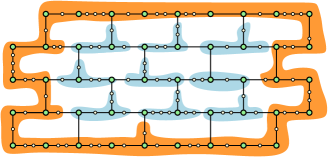
For every we denote by the graph and to be the graph Now consider the collection and observe that the graphs in are connected subgraphs of and their vertex sets form a partition of We call the canonical partition of Also, we call every an internal bag of while we refer to as the external bag of See Figure 2 for an illustration of the notions defined above. For every we say that a set is an -internal bag of if does not contain any vertex of the first layers of Notice that the -internal bags of are the internal bags of
Let be a flatness pair of a graph Consider the canonical partition of We enhance the graphs of so to include in them all the vertices of by applying the following procedure. We set and, as long as there is a vertex that is adjacent to a vertex of a graph update where Since is a connected graph, in this way we define a partition of the vertices of into subsets inducing connected graphs. We call the that contains as a subgraph the external bag of and we denote it by while we call internal bags of all graphs in Moreover, we enhance by adding all vertices of in its external bag, i.e., by updating We call such a partition a -canonical partition of Notice that a -canonical partition of is not unique, since the sets in can be “expanded” arbitrarily when introducing vertex .
Let be a flatness pair of a graph of height for some and be a -canonical partition of For every we say that a set is an -internal bag of if it contains an -internal bag of as a subgraph.
Next we identify a combinatorial structure that guarantees the existence of a set of vertices that intersects every solution of -M-Deletion with input This will permit branching on simpler instances of the form Recall that is the minimum apex number of a graph in The following result is proved in [SauST21kapiI].
Proposition \theproposition.
There exist three functions such that if is a finite set of graphs, is a graph, is a subset of is a flatness pair of of height at least is a -canonical partition of is a subset of vertices of that are adjacent, in to vertices of at least -internal bags of and then for every set of size at most such that it holds that Moreover, and where and
The next result is also proved in [SauST21kapiI] and intuitively states that, given a flatness pair of “big enough” height and a -canonical partition of we can find a “packing” of subwalls of that are inside some central part of and that the vertex set of every internal bag of intersects the vertices of the flaps in the influence of at most one of these walls. We will use this result in the case where the set of Subsection 4.2 is “small”, i.e., there are only “few” vertices in that have “big enough” degree with respect to the central part of the canonical partition, and therefore Subsection 4.2 cannot justify branching. Following the latter condition and Subsection 4.2, we will be able to find a flatness pair with “few” apices so as to build irrelevant vertex arguments inside its compass.
Proposition \theproposition.
There exists a function such that if is an odd integer, is a graph, is a flatness pair of of height at least and is a -canonical partition of then there is a collection of -subwalls of such that
-
•
for every is a subgraph of and
-
•
for every with there is no internal bag of that contains vertices of both and
Moreover,
5 The general algorithm
In this section we present the general algorithm for -M-Deletion. The existence of this algorithm proves Section 1. In Subsection 5.1, we explain how to employ the iterative compression technique so as to ask for an algorithm for a new, more convenient to solve, problem and, in Subsection 5.2, we develop an algorithm for this new problem.
5.1 Iterative compression
In order to prove Section 1, we apply the iterative compression technique (introduced in [ReedSV04find]; see also [CyganFKLMPPS15para]) and we give a -time algorithm for the following problem.
-M-Deletion-Compression
Input: A graph a and a set of size such that
Objective: Find, if exists, a set of size at most such that
In other words, given an input of -M-Deletion-Compression, we have at hand a graph and a “slightly larger than ” hitting set , and we aim to find a hitting set of size at most that is a certificate that is a yes-instance of -M-Deletion. Given this set we can directly assume that does not contain a big clique as a minor and therefore we can deal with this minor-free graph, and thus, due to Subsection 3.3, we can obtain either a tree decomposition of of “small” width (and solve the problem using the dynamic programming algorithm of [BasteST20acom]), or a flat wall on top of which we build our branching and irrelevant vertex technique arguments. In this way, we manage to avoid the “big clique” possible output of Subsection 3.3. However, this swifting from -M-Deletion to -M-Deletion-Compression comes together with an extra linear factor in the running time of the algorithm, as observed in the following (see [CyganFKLMPPS15para]).
Observation \theobservation.
If there is an algorithm solving -M-Deletion-Compression in -time, then there exists an algorithm solving -M-Deletion in -time.
In Subsection 5.2 we prove that -M-Deletion-Compression can be solved in -time (Subsection 5.2). This along with Subsection 5.1 yield Section 1.
5.2 The algorithm
In this subsection we present the algorithm solving -M-Deletion-Compression.
We set where f3.4 is the number of different folios given in Subsection 3.4 and f4.1 is the function given in Subsection 4.1, in order to find an irrelevant vertex.
Lemma \thelemma.
Let be a finite collection of graphs. There is an algorithm solving -M-Deletion-Compression in -time, where , and
Proof.
For simplicity, in this proof, we use instead of instead of instead of instead of and recall that and Also, we set