Diversity in Action:
General-Sum Multi-Agent Continuous Inverse Optimal Control

Abstract

Traffic scenarios are inherently interactive. Multiple decision-makers predict the actions of others and choose strategies that maximize their rewards. We view these interactions from the perspective of game theory which introduces various challenges. Humans are not entirely rational, their rewards need to be inferred from real-world data, and any prediction algorithm needs to be real-time capable so that we can use it in an autonomous vehicle (AV). In this work, we present a game-theoretic method that addresses all of the points above. Compared to many existing methods used for AVs, our approach does 1) not require perfect communication, and 2) allows for individual rewards per agent. Our experiments demonstrate that these more realistic assumptions lead to qualitatively and quantitatively different reward inference and prediction of future actions that match better with expected real-world behaviour.

1 INTRODUCTION

One of the most pressing problems that need to be solved to realize autonomous driving in urban environments is the interaction with vulnerable road users such as pedestrians and cyclists. Merely extrapolating the current velocity vector of a pedestrian fails to account for behavioural changes caused by interactions with traffic participants and the environmental layout (traffic lights, zebra crossings, obstacles). Existing work (Kretzschmar et al., 2016; Pfeiffer et al., 2016; Sadigh et al., 2018; Schwarting et al., 2019a; Ma et al., 2017) in the domain of intelligent vehicles may describe these kinds of social interactions in terms of Markov Decision Processes (MDP), i.e. a framework where each agent (human) is maximizing a reward (avoid collision, be considerate). Three aspects are crucial when using MDPs to model human interactions. One is inferring the correct reward function from real-world data, another is to account for bounded rationality, and finally, we want real-time predictions given a reward function.

Reward Inference: One way of inferring rewards from multi-agent data is to fix the observed actions of the other agents, i.e. decoupling the actions from the other agents from one’s own (Schwarting et al., 2019a; Sadigh et al., 2018). Treating other agents as dynamic obstacles reduces the problem to that of a single agent. Another approach is to assume that all agents are controlled by one ”brain” (Kretzschmar et al., 2016; Pfeiffer et al., 2016). Therefore, communication between agents is instant, and they may coordinate their actions perfectly. Additionally, all agents optimize the same (cooperative) reward function. While this assumption simplifies computations, it represents an overly altruistic view of the world.

Bounded Rationality: Humans are boundedly rational (Wright & Leyton-Brown, 2010). Instead of executing an action that leads to the highest expected reward, humans may choose another action that rewards less. In other words, the probability of selecting an action increases with the expected reward of that action. Humans do not follow deterministic paths in traffic scenarios. Instead, they show natural variation in their decision making. (Schwarting et al., 2019a; Fridovich-Keil et al., 2019a; Sadigh et al., 2018) argue from the deterministic perspective that agents maximize their expected reward as much as possible. We aim for a prediction algorithm that takes bounded rationality into account.

Another term that relates to the same concept is probability matching. (Eysenbach & Levine, 2019) discusses probability matching in maximum-entropy reinforcement learning and the connection to human and animal decision making. Also, we may refer to the behaviour of an agent as sub-optimal, meaning the same concept.

Operational Constraints: A prediction algorithm should be capable of running efficiently (preferably in real-time) and work in continuous action and state spaces. (Fridovich-Keil et al., 2019a) demonstrate a multi-agent algorithm that is real-time capable. The underlying reason for the efficiency is that the algorithm belongs to the family of linear quadratic regulator (LQR) methods.

Contributions: In this work, we address the challenges outlined above. We present a novel algorithm that

• learns the reward functions of a diverse set of agents. It does not assume the other agents as dynamic obstacles, and it does not assume instant communication between agents.

• accounts for variation in the decisions of an agent because it belongs to the family of maximum-entropy algorithms.

• can be adapted for prediction tasks, with the potential of running in real-time as it is related to LQR methods.

In particular,

• we extend the continuous inverse optimal control (CIOC) (Levine & Koltun, 2012) algorithm to the general-sum two-agent setting

• we verify the algorithm on simulations and show its usefulness. In particular, our algorithm allows us to choose different reward functions for each agent. Additionally, we observe a significant difference in the deduced reward and predictions when not assuming instant communication.

2 Related Work

We focus on work that deals with traffic interactions involving pedestrians, or that could be easily applied to such interactions. For a comprehensive overview of the literature on predicting the intentions of pedestrians see (Rudenko et al., 2019). We focus on the multi-agent generalizations of Markov Decision Processes (MDPs) where the agent (e.g. pedestrian) executes actions (step to the right) to maximize a reward (avoid collision). A useful extension of the standard MDP framework to the maximum-entropy framework can describe boundedly rational behaviour of humans more closely (see e.g. (Kitani et al., 2012)).

In the following sub-sections, we outline other work close to ours, considering (real-time) multi-agent games in continuous action and state spaces that model interactions of robots (or humans) with humans in traffic like scenarios.

Multi-Agent Games: (Sadigh et al., 2018; Schwarting et al., 2019a) consider so-called Stackelberg games between cars in continuous state and action spaces where the agents take turns and communicate their actions to the other agents before executing them. This simplifies the computational complexity of the problem significantly since it is sequential and deterministic in nature. Both publications infer the reward functions from real-world data using CIOC (Levine & Koltun, 2012). Though, other agents are reduced to dynamic obstacles simplifying the reward inference (i.e. non reacting).

The approaches of (Schwarting et al., 2019b; Fridovich-Keil et al., 2019b, a) are inspired by the iLQG algorithm and the well-established solutions to linear quadratic games (see for example (Basar & Olsder, 1999)). They can deal with non-linear dynamics and non-linear cost functions in multi-agent dynamic games. In contrast to our work, (Fridovich-Keil et al., 2019b, a; Schwarting et al., 2019b) do not consider boundedly rational agents and reward inference.

Bounded Rationality: The notion of bounded rationality has a long tradition in both artificial intelligence (Simon, 1955; Russell, 1997; Zilberstein, 2011; Rubinstein, 1986; Halpern et al., 2014) and (behavioral) game theory (McKelvey & Palfrey, 1995; Rubinstein, 1998; Wright & Leyton-Brown, 2010). In particular, we will use a model of bounded rationality that is very close to the quantal response equilibrium (McKelvey & Palfrey, 1995). Our contribution here can be seen as the ability to approximate such a QRE, in continuous games, while also inferring the rewards from data.

Maximum Entropy Inverse Reinforcement Learning: Also, in the context of RL, people have considered notions of boundedly rational agents. (Ziebart et al., 2008) introduced maximum-entropy inverse reinforcement learning (MaxEntIRL) to obtain the rewards from agents that act boundedly rational. The most daunting task in MaxEntIRL for high dimensional continuous action and state spaces (i.e. no dynamic programming) is the derivation of the partition function $Z=\int p(\tau)\exp(r(\tau))$. (Kuderer et al., 2013) approximate the distribution over trajectories with weighted sums of delta-functions representing the observed data points, optimizing the data likelihood by gradient ascent. A more advanced algorithm - which we will use in this paper - is the use of the Laplace approximation (second-order Taylor expansion) around the observed data points that models the curvature of the reward function (Levine & Koltun, 2012; Dragan & Srinivasa, 2013). Another possibility is a sampling-based approximation by, e.g. Monte Carlo methods (Kretzschmar et al., 2016; Pfeiffer et al., 2016; Xu et al., 2019). In general, this corresponds to solving the full reinforcement learning problem in an inner loop of the inverse reinforcement learning algorithm (Finn et al., 2016).

3 BACKGROUND

We are considering a two-agent stochastic game with shared states $x_{t}$, agent specific actions $u_{it}$, $u_{jt}$ (i,j - agent index), agent specific rewards $r_{i}(x_{t},u_{it},u_{jt})$ and stochastic transitions $p(x_{t}|u_{it},u_{jt},x_{t-1})$ to the $x_{t}$ given the actions $u_{kt}$ and state $x_{t-1}$. In general, both the transitions and the reward function depend on the actions of both agents.

Also, the rewards of the agents are discounted with a discount factor $\gamma$. In the following, we give an overview of the most important formulas for the single-agent case. These will translate to the two-agent setting naturally.

Given a state $x_{t-1}$ at time-step $t-1$ and an action $u_{t}$, an agent will transition to the next state according to the stochastic environment transitions $p(x_{t}|x_{t-1},u_{t})$. The agent will also receive a reward $r(x_{t},u_{t})$ depending on the action $u_{t}$ and the state $x_{t}$ that the environment (including the agent) transitions to. In this work, we assume that an agent does not act fully rational and chooses sub-optimal actions. A natural description of this type of bounded rationality is the maximum-entropy (MaxEnt) framework (Ziebart et al., 2008) which can be used to describe the sub-optimal decisions of humans (e.g. (Kitani et al., 2012)). In the MaxEnt framework, a trajectory is sampled from a probability distribution given by

$$p(\tau)=\Pi_{t}p(x_{t}|x_{t-1},u_{t})\exp(r(x_{t},u_{t}))$$ (1)

with the trajectory $\tau$ corresponding to the sequence of actions $u_{t}$ and states $x_{t}$ over multiple time-steps $t$. The policy $\pi(u_{t}|x_{t-1})$ of an agent, i.e. the conditional pdf that describes the most likely actions $u_{t}$ that an agent takes given its current state $x_{t-1}$ depends on the Q-function

$$\pi(u_{t}|x_{t-1})=\frac{\exp(Q(x_{t-1},u_{t}))}{\int\exp(Q(x_{t-1},u_{t}^{\prime})du_{t}^{\prime})}$$ (2)

The Q-function may be derived by performing dynamic programming, iterating over the soft-Bellman equation until convergence.

$$Q(x_{t-1},u_{t})=\int p(x_{t}^{\prime}|u_{t},x_{t-1})\Big{(}r(x_{t}^{\prime},u_{t})+\\ \gamma\log\int\exp(Q(x_{t}^{\prime},u_{t+1}^{\prime}))du^{\prime}_{t+1}\Big{)}dx_{t}^{\prime}$$ (3)

The second term inside the first integral is the value function.

$$V(x_{t})=\log\int\exp(Q(x_{t},u^{\prime}_{t+1}))du^{\prime}_{t+1}$$ (4)

The reason we refer to (3) as the soft-Bellman equation is the soft-maximization operator $\log\int\exp$. In contrast, the standard Bellman equation employs the ”hard” maximization operator $\max$. A connection can be established by scaling the reward function and considering the limit of $\lim_{\alpha\rightarrow+\infty}(\alpha r)$ which will recover the ”hard” maximization in the soft-Bellman equation and a policy that satisfies the standard Bellman equation given the unscaled reward function. Please refer to the excellent tutorial on maximum-entropy reinforcement learning and its connection to probabilistic inference (Levine, 2018) for a thorough derivation of the soft-Bellman equation and its connection to (1).

In the following sections, we will only consider finite horizon problems, i.e. each agent will collect rewards for a limited amount of time. Additionally, we set the discount factor to $\gamma=1$.

4 General-Sum Multi-Agent Continuous Inverse Optimal Control

We extend CIOC to the two-agent setting where each agent may receive a different reward. A major difference to the derivation of CIOC is the environment transitions that are not deterministic anymore. We assume that the other agent is part of the environment and acts according to a stochastic policy. The iterative nature of the algorithm bears a resemblance to (Nair et al., 2003), though, we update the policies in parallel (not alternating) while also being able to handle continuous states and actions. A major advantage of CIOC and its extension is the relative ease of inferring the reward parameters from demonstrations. We can backpropagate the gradients directly through the policy, eliminating the need to run a complex deep reinforcement learning algorithm every time we update the reward parameters.

We will present three algorithms that are interconnected. General-Sum Multi-Agent Continuous Inverse Optimal Control (GS-CIOC) (algorithm 13) that returns policies for quadratic rewards and linear environment transitions. For non-quadratic rewards and non-linear transitions, Iterative GS-CIOC can be used (algorithm 7) to obtain locally optimal policies. It uses GS-CIOC as a sub-routine. Finally, the reward inference algorithm 6 uses GS-CIOC for obtaining local policy approximations around observed real-world data for any type of reward functions and transitions.

Two-Agent Soft-Bellman Equation

We assume that all agents choose their actions in accordance with (1) which directly raises the question how they deal with the presence of other agents. Here, the other agent is part of the environment, similar to the multi-agent setting in interacting Partially Observable Markov Decision Processes (POMDPs) as described by (Gmytrasiewicz & Doshi, 2005). Let $u_{it}$, $u_{jt}$ be the actions of agent i and j respectively. We assume the environment transitions to be deterministic, i.e. $p(x_{t}|x_{t-1},u_{it},u_{jt})$ is a deterministic function. The reward function of agent i may depend on the action of agent j, i.e. $r_{i}(x_{t},u_{it},u_{jt})$, though $u_{jt}$ is not known to agent i at $t-1$. Therefore, for argument’s sake, we define a new state variable $\tilde{x}_{t}=[x_{t},u_{jt}]$ and the corresponding stochastic environment transitions $p(\tilde{x}_{t}|\tilde{x}_{t-1},u_{it}):=p(x_{t},u_{jt}|x_{t-1},u_{jt-1},u_{it})$. The soft-Bellman equation for agent i is as follows

$$Q_{i}(\tilde{x}_{t-1},u_{it})=\int p(\tilde{x}_{t}|\tilde{x}_{t-1},u_{it})\Big{(}r_{i}(\tilde{x}_{t},u_{it})\\ +\gamma\log\int\exp(Q_{i}(\tilde{x}_{t},u_{it+1}))du_{it+1}\Big{)}d\tilde{x}_{t}$$ (5)

The agent decides on its action based on $x_{t}$, not $\tilde{x}_{t}$. Thus, we can drop the $\tilde{x}_{t}$ dependency in the Q-function. Also, we can expand the environment transitions $p(\tilde{x}_{t}|\tilde{x}_{t-1},u_{it})=p(x_{t}|x_{t-1},u_{it},u_{jt})\pi_{j}(u_{jt}|x_{t-1})$, with $\pi_{j}$ being the policy of agent j. The soft-Bellman equation can now be reformulated as

$$Q_{i}(x_{t-1},u_{it})=\\ \int p(x_{t}|x_{t-1},u_{it},u_{jt})\pi_{j}(u_{jt}|x_{t-1})\Big{(}r_{i}(x_{t},u_{it},u_{jt})\\ +\gamma\log\int\exp(Q_{i}(x_{t},u_{it+1}))du_{it+1}\Big{)}du_{jt}dx_{t}$$ (6)

Solving the Bellman-equation for high-dimensional continuous state and action spaces is in general intractable. Tackling this problem employs many researchers in the fields of reinforcement learning and optimal control. Here, we make use of the so-called Laplace approximation that deals with the difficulty of calculating the partition function $\int\Pi_{t}p(x_{t}|x_{t-1},u_{t})\exp(r(x_{t},u_{t}))du_{t}dx_{t}$ by approximating the reward function with a second-order Taylor expansion. (Levine & Koltun, 2012) developed the Continuous Inverse Optimal Control (CIOC) algorithm based on this approximation. Though, their approach is limited to the single-agent case with deterministic environment transitions. We will show how to extend their algorithm to the two-agent setting.

Value Recursion Formulas

Algorithm 1 GS-CIOC

  Input: Reference trajectories $\tau_{k}$, $k\in\{i,j\}$

  Taylor expansion (8) of rewards along $\tau_{k}$

  Initialize $V_{k}(x_{T})\leftarrow 0$

  for $t\leftarrow T$ to $1$ do

     {Update Gaussian policy:}

     $\mu_{kt}\leftarrow$ Solve (17) for mean action

     $\tilde{M}_{(kk)t}\leftarrow$ Determine precision matrix (15)

     {Recompute value function, given updated policy:}

     if $t>1$ then

        $V_{k}(x_{t-1})\leftarrow$ Value recursion (22) - (26)

     end if

  end for

  Return: Policies $\pi_{i}$ and $\pi_{j}$

The procedure that we obtain in this section is illustrated in algorithm 13. We take a reference trajectory $\tau_{k}$ - a sequence of states $x_{t}$ and actions $u_{kt}$ - of each agent $k\in(i,j)$ and approximate the reward function $r_{k}$ close to the reference trajectory. This will allow us to derive a local policy approximation $\pi_{k}$ - an approximation that works best if the agent stays close to the reference trajectory - by working our way from the end of the reference trajectory to the beginning calculating the value function $V_{k}(x_{t})$ for each time-step. In other words, the formulas are recursive in nature. Where does the reference trajectory come from? It may be a randomly chosen state and action sequence, or it may represent actual observation data.

We sketch the derivation of algorithm 13 starting at the final time-step (the horizon) of the reference trajectories $\tau_{i}$, $\tau_{j}$. Here the Q-function of agent i and by extension the policy $\pi_{i}$ can be calculated as follows

$$Q_{i}(\bar{x}_{T-1},\bar{u}_{iT})=\int p(\bar{x}_{T}|\bar{x}_{T-1},\bar{u}_{iT},\bar{u}_{jT})\\ \pi_{j}(\bar{u}_{jT}|\bar{x}_{T-1})r_{i}(\bar{x}_{T},\bar{u}_{iT},\bar{u}_{jT})d\bar{u}_{jT}d\bar{x}_{T}$$ (7)

Even though $p(\bar{x}_{T}|\bar{x}_{T-1},\bar{u}_{iT},\bar{u}_{jT})$ is deterministic, the integral is intractable in general. We circumvent this problem by approximating the reward function $r_{i}$ using a second-order Taylor expansion around the fixed reference trajectories.

$$r_{i}(\bar{x}_{t},\bar{u}_{it},\bar{u}_{jt})\approx r_{it}+\bar{x}_{jt}^{T}\Big{(}\hat{H}_{(ji)t}\bar{x}_{it}\Big{)}+\bar{u}^{T}_{jt}\Big{(}\tilde{H}_{(ji)t}\bar{u}_{it}\Big{)}\\ +\sum_{k=1}^{2}\Bigg{[}\bar{x}_{kt}^{T}\Big{(}\frac{1}{2}\hat{H}_{(kk)t}\Big{)}\bar{x}_{kt}+\bar{u}^{T}_{kt}\Big{(}\frac{1}{2}\tilde{H}_{(kk)t}\Big{)}\bar{u}_{kt}+\\ \bar{u}_{kt}^{T}\tilde{g}_{kt}+\bar{x}_{kt}^{T}\hat{g}_{kt}\Bigg{]}$$ (8)

$H$ and $g$ refer to the Hessians and gradients w.r.t the states and actions of both agents.

$$\hat{H}_{(nm)t} =\frac{\partial^{2}r_{i}}{\partial\bar{x}_{nt}\partial\bar{x}_{mt}},\qquad\tilde{H}_{(nm)t}=\frac{\partial^{2}r_{i}}{\partial\bar{u}_{nt}\partial\bar{u}_{mt}}$$ (9)

$$\hat{g}_{nt} =\frac{\partial r_{i}}{\partial\bar{x}_{nt}},\qquad\tilde{g}_{nt}=\frac{\partial r_{i}}{\partial\bar{u}_{nt}}$$ (10)

The reward function is now quadratic with

$$\bar{x}_{t}=x_{t}-x_{t}^{*},\qquad\bar{u}_{kt}=u_{kt}-u_{kt}^{*}$$ (11)

where $x^{*}$ and $u^{*}$ refer to the fixed reference trajectories. The state $\bar{x}_{t}=[\bar{x}_{it},\bar{x}_{jt}]$ is split into the agent specific sub-states which are directly controlled by each agent.

We need one additional approximation to solve the integral in (7). Namely, we linearize the dynamics

$$\bar{x}_{kt} =A_{kt}\bar{x}_{kt-1}+B_{kt}\bar{u}_{kt}$$ (12)

$$A_{kt} =\frac{\partial\bar{x}_{kt}}{\partial\bar{x}_{kt-1}},\qquad B_{kt}=\frac{\partial\bar{x}_{kt}}{\partial\bar{u}_{kt-1}}$$ (13)

Applying the linearization and the quadratic approximation of the reward function turns (7) into a tractable integral. In particular, $Q_{iT}$ is quadratic in the actions $\bar{u}_{iT}$. Therefore, the policy of agent i is a Gaussian policy. The same is true for agent j since we apply the same approximations, i.e. $\pi_{j}$ is a Gaussian policy. The mean of that policy is (general result)

$$\mu_{it}=-\tilde{M}^{-1}_{(ii)t}\Big{(}\tilde{g}_{it}+\tilde{H}_{(ij)t}\mu_{jt}+B^{T}_{it}\hat{q}_{ijt}+B^{T}_{it}\hat{Q}_{(ii)t}A_{it}\bar{x}_{it-1}\Big{)}$$ (14)

$\tilde{M}_{(ii)t}$ is the precision matrix of the Gaussian policy of agent i.

$$\tilde{M}_{(nm)t}=B_{nt}^{T}\hat{Q}_{(nm)t}B_{mt}+\tilde{H}_{(nm)t}$$ (15)

Additional definitions of symbols used in the equations above

$$\hat{q}_{it}=\hat{g}_{it}+\hat{v}_{it},\qquad\hat{Q}_{(nm)t}=\hat{H}_{(nm)t}+\hat{V}_{(nm)t}$$ (16)

(14) is a system of linear equations in $\mu_{it}$ and $\mu_{jt}$ of the form $Ax=b$.

$$\Big{[}\delta_{ij}^{(i)}\Big{(}\tilde{M}_{(jj)t}^{-1}\Big{)}^{(j)}\delta_{ji}^{(j)}-\Big{(}\tilde{M}_{(ii)t}\Big{)}^{(i)}\Big{]}\mu_{it}=$$

$$\alpha_{i}^{(i)}-\delta_{ij}^{(i)}\Big{(}\tilde{M}_{(jj)t}^{-1}\Big{)}^{(j)}\alpha_{j}^{(j)}+$$

$$\Big{(}\beta_{i}^{(i)}-\delta_{ij}^{(i)}\Big{(}\tilde{M}_{(jj)t}^{-1}\Big{)}^{(j)}\gamma_{ji}^{(j)}\Big{)}\bar{x}_{it-1}+$$

$$\Big{(}\gamma_{ij}^{(i)}-\delta_{ij}^{(i)}\Big{(}\tilde{M}_{(jj)t}^{-1}\Big{)}^{(j)}\beta_{j}^{(j)}\Big{)}\bar{x}_{jt-1}$$ (17)

with

$$\alpha_{i}^{(i)}= \Big{[}\tilde{g}_{it}+B_{it}^{T}\hat{q}_{it}\Big{]},\qquad\beta_{i}^{(i)}=B_{it}^{T}\hat{Q}_{(ii)t}A_{it}$$ (18)

$$\gamma_{ij}^{(i)}= B_{it}^{T}\hat{Q}_{(ij)t}A_{jt},\qquad\delta_{ij}^{(i)}=\tilde{M}_{(ij)t}$$ (19)

The ⁽ⁱ⁾ index indicates which agent the derivatives/ value functions refer to. We do not only recover the mean of agent j but also that of agent i.

At last, we calculate the value function using equation (4). The Q-function is a quadratic polynomial in the states and actions. Therefore, the integral is tractable, and we end up with a value function with the following structure

$$V_{i}(\bar{x}_{T})=\bar{x}^{T}_{jT}\Big{(}\hat{V}_{(ji)T}\bar{x}_{iT}\Big{)}+\\ \sum_{k=1}^{2}\left[\bar{x}^{T}_{kT}\Big{(}\frac{1}{2}\hat{V}_{(kk)T}\Big{)}\bar{x}_{kT}+\bar{x}^{T}_{kT}\hat{v}_{kT}\right]+const$$ (20)

How do we obtain the $\hat{V}$ and $\hat{v}$ matrices? We collect all the terms that are quadratic or linear in $\bar{x}_{kt}$. The general result is given in equation (22) onward.

Now, that we know $V_{iT}$, we apply the same procedure to the previous time step, i.e. the calculations are repetitive. In short, we derive the Q-function of the next time-step ($T-1$).

$$Q_{i}(\bar{x}_{T-2},\bar{u}_{iT-1})=\\ \int p(\bar{x}_{T-1}|\bar{x}_{T-2},\bar{u}_{iT-1},\bar{u}_{jT-1})\pi_{j}(\bar{u}_{jT-1}|\bar{x}_{T-2})\Big{(}\\ r(\bar{x}_{T-1},\bar{u}_{iT-1},\bar{u}_{jT-1})+V_{i}(\bar{x}_{T})\Big{)}d\bar{u}_{jT-1}d\bar{x}_{T-1}$$ (21)

Given the reward approximation, the linearization of the dynamics and the quadratic state dependency of the value function $V_{iT}$ in equation (20) this integral is tractable again. Working our way along the full trajectory, we obtain recursive formulas for the value functions (meaning the $\hat{V}$ matrices and $\hat{v}$ vectors in (20)). Due to space constraints, we will state the results and refer the interested reader to the supplementary material.

$$\hat{V}_{(ii)t-1} =\Pi_{jt}^{T}\Big{[}\tilde{M}_{(jj)t}-\tilde{M}_{(ji)t}\tilde{M}_{(ii)t}^{-1}\tilde{M}_{(ij)t}]\Pi_{jt}$$

$$+ \Big{[}A_{it}^{T}\hat{Q}_{(ij)t}B_{jt}-A_{it}^{T}\hat{Q}_{(ii)t}B_{it}\tilde{M}_{(ii)t}^{-1}\tilde{M}_{(ij)t}\Big{]}\Pi_{jt}$$

$$+ \Pi_{jt}^{T}\Big{[}A_{it}^{T}\hat{Q}_{(ij)t}B_{jt}-A_{it}^{T}\hat{Q}_{(ii)t}B_{it}\tilde{M}_{(ii)t}^{-1}\tilde{M}_{(ij)t}\Big{]}^{T}$$

$${\color[rgb]{0,0,1}+} {\color[rgb]{0,0,1}A^{T}_{it}\hat{Q}_{(ii)t}A_{it}}{\color[rgb]{0,0,1}-A_{it}^{T}\hat{Q}_{(ii)t}^{T}B_{it}\tilde{M}_{(ii)t}^{-1}B_{it}^{T}\hat{Q}_{(ii)t}A_{it}}$$ (22)

$$\hat{V}_{(jj)t-1} =\Omega^{T}_{jt}\Big{[}\tilde{M}_{(jj)t}-\tilde{M}_{(ji)t}\tilde{M}_{(ii)t}^{-1}\tilde{M}_{(ij)t}\Big{]}\Omega_{jt}$$

$$+ \Big{[}A^{T}_{jt}\hat{Q}_{(jj)t}B_{jt}-A^{T}_{jt}\hat{Q}_{(ji)t}B_{it}\tilde{M}_{(ii)t}^{-1}\tilde{M}_{(ij)t}\Big{]}\Omega_{jt}$$

$$+ \Omega_{jt}^{T}\Big{[}A^{T}_{jt}\hat{Q}_{(jj)t}B_{jt}-A^{T}_{jt}\hat{Q}_{(ji)t}B_{it}\tilde{M}_{(ii)t}^{-1}\tilde{M}_{(ij)t}\Big{]}^{T}$$

$$+ A_{jt}^{T}\hat{Q}_{(jj)t}A_{jt}-A_{jt}^{T}\hat{Q}_{(ji)t}B_{it}\tilde{M}_{(ii)t}^{-1}B_{it}^{T}\hat{Q}_{(ij)t}A_{jt}$$ (23)

$$\hat{V}_{(ji)t-1} =\Omega_{jt}^{T}\Big{[}\tilde{M}_{(jj)t}-\tilde{M}_{(ji)t}\tilde{M}_{(ii)t}^{-1}\tilde{M}_{(ij)t}\Big{]}\Pi_{jt}$$

$$+ \Omega_{jt}^{T}\Big{[}A_{it}^{T}\hat{Q}_{(ij)t}B_{jt}-A_{it}^{T}\hat{Q}_{(ii)t}B_{it}\tilde{M}_{(ii)t}^{-1}\tilde{M}_{(ij)t}\Big{]}^{T}$$

$$+ \Big{[}A_{jt}^{T}\hat{Q}_{(jj)t}B_{jt}-A_{jt}^{T}\hat{Q}_{(ji)t}B_{it}\tilde{M}_{(ii)t}^{-1}\tilde{M}_{(ij)t}\Big{]}\Pi_{jt}$$

$$+ A_{jt}^{T}\hat{Q}_{(ji)t}A_{it}-A_{jt}^{T}\hat{Q}_{(ji)t}B_{it}\tilde{M}_{(ii)t}^{-1}B_{it}^{T}\hat{Q}_{(ii)t}A_{it}$$ (24)

$$\hat{v}_{jt-1} =\Omega_{jt}^{T}\Big{[}\tilde{M}_{(jj)t}-\tilde{M}_{(ji)t}\tilde{M}_{(ii)t}^{-1}\tilde{M}_{(ij)t}\Big{]}\nu_{jt}$$

$$+ \Big{[}A^{T}_{jt}\hat{Q}_{(jj)t}B_{jt}-A^{T}_{jt}\hat{Q}_{(ji)t}B_{it}\tilde{M}_{(ii)t}^{-1}\tilde{M}_{(ij)t}\Big{]}\nu_{jt}$$

$$+ \Omega_{jt}^{T}\Big{(}\tilde{g}_{jt}+B_{jt}^{T}\hat{q}_{jt}-\tilde{M}_{(ji)t}\tilde{M}_{(ii)t}^{-1}\Big{[}\tilde{g}_{it}+B_{it}^{T}\hat{q}_{it}\Big{]}\Big{)}$$

$$+ A_{jt}^{T}\hat{q}_{jt}-A_{jt}^{T}\hat{Q}_{(ji)t}B_{it}\tilde{M}^{-1}_{(ii)t}[\tilde{g}_{it}+B^{T}_{it}\hat{q}_{it}]$$ (25)

$$\hat{v}_{it-1} =\Pi_{jt}^{T}\Big{[}\tilde{M}_{(jj)t}-\tilde{M}_{(ji)t}\tilde{M}_{(ii)t}^{-1}\tilde{M}_{(ij)t}\Big{]}\nu_{jt}$$

$$+ \Big{[}A^{T}_{it}\hat{Q}_{(ij)t}B_{jt}-A^{T}_{it}\hat{Q}_{(ii)t}B_{it}\tilde{M}_{(ii)t}^{-1}\tilde{M}_{(ij)t}\Big{]}\nu_{jt}$$

$$+ \Pi_{jt}^{T}\Big{(}\tilde{g}_{jt}+B_{jt}^{T}\hat{q}_{jt}-\tilde{M}_{(ji)t}\tilde{M}_{(ii)t}^{-1}\Big{[}\tilde{g}_{it}+B_{it}^{T}\hat{q}_{it}\Big{]}\Big{)}$$

$${\color[rgb]{0,0,1}+} {\color[rgb]{0,0,1}A^{T}_{it}\hat{q}_{it}}{\color[rgb]{0,0,1}-A^{T}_{it}\hat{Q}_{(ii)t}B_{it}\tilde{M}^{-1}_{it}\Big{[}\tilde{g}_{it}+B^{T}_{it}\hat{q}_{it}\Big{]}}$$ (26)

The parts of the formulas that are highlighted in blue correspond to the single agent value recursion formulas from (Levine & Koltun, 2012). If the reward is a single agent reward function, the value recursion formulas will reduce to the highlighted parts.

$\Pi$ and $\Omega$ refer to the reactive policy of agent j, i.e. they encode how agent j will react to deviations in the position of agent i (or agent j itself). The mean action of agent j is given by

$$\mu_{jt}=\nu_{jt}+\Pi_{jt}\bar{x}_{it-1}+\Omega_{jt}\bar{x}_{jt-1}$$ (27)

Iterative GS-CIOC

Algorithm 2 Iterative GS-CIOC

  Input: Initial trajectories $\tau_{i}$, $\tau_{j}$ learning rate $\eta$

  repeat

     $\pi_{i}$, $\pi_{j}\leftarrow$ GS-CIOC( $\tau_{i}$, $\tau_{j}$)

     {Update $\tau_{i}$, $\tau_{j}$}

     Roll-out Gaussian policies with scaled mean $\eta\mu_{kt}$ and covariance = 0 (i.e. deterministic policy)

  until max iterations

  Return: Policies $\pi_{i}$ and $\pi_{j}$

We can use the algorithm described above to generate predictions (rollout policy), but this will only result in globally optimal solutions for quadratic rewards and linear (deterministic) environment transitions. In that case, the Taylor expansion around any given reference trajectory is exact everywhere. If the rewards are not quadratic, the quadratic approximation of the reward and value function is, of course, inaccurate and holds only close to a given reference trajectory. Though, we can execute GS-CIOC iteratively to find local optima (with no convergence guarantee). We start with an initial trajectory and approximate the rewards and dynamics locally. We obtain a Gaussian policy by executing the value recursion described above and update the trajectory by following the policy up to a learning rate $\eta$. One possibility is to scale the mean of the policy via $\eta\mu$. This way, we can control how much the update deviates from the reference trajectory. This algorithm resembles the iLQG algorithm and has been explored recently for the multi-agent setting in dynamic games by (Schwarting et al., 2019b; Fridovich-Keil et al., 2019b). We illustrate the procedure in algorithm 7.

In general, it is important to note that neither (Schwarting et al., 2019b) nor (Fridovich-Keil et al., 2019b), nor our approach recover Nash-equilibria (NE) since the best responses computed are approximations that work only locally w.r.t. the current reference trajectory. The agents might not find a better response which lies far away from the current reference trajectory. See also (Oliehoek et al., 2019) for a discussion on why local NE can be far from a NE.

5 Recovering Reward Parameters

Until now, we have discussed how to construct a local policy given a set of reference trajectories and a reward function (see algorithms 13 and 7). However, since our goal is to use the predicted behaviours in real-life traffic interactions, we need the capability to infer the parameters $\theta$ of a reward function that captures human behaviour. For this purpose, we present an algorithm that can be run before deploying algorithm 7, to infer realistic rewards. Specifically, given observation data of, e.g. a pedestrian interacting with a car, we can infer the reward parameters by maximizing the log-likelihood of the observed data

$$\theta^{*} =$$

$$\arg \max_{\theta}\frac{1}{|\tau|}\sum_{\tau,(u,x)\in\tau}\ln p_{\theta}(x_{i0:T-1},x_{j0:T-1},u_{i1:T},u_{j1:T})$$

$$=\arg\max_{\theta}\frac{1}{|\tau|}\sum_{\tau,(u,x)\in\tau}\Bigg{(}\sum_{t}\ln\pi_{i,\theta}(u_{it}|x_{it-1},x_{jt-1})$$

$$+\sum_{t}\ln\pi_{j,\theta}(u_{jt}|x_{it-1},x_{jt-1})\Bigg{)}$$ (28)

$\theta$ refers to the reward parameters and $|\tau|$ to the number of trajectories $\tau$ in the data set. $\pi_{i,\theta}$ corresponds to the policy of agent i (e.g. pedestrian) and is calculated with GS-CIOC. Indeed, it is possible to perform backpropagation through the entire GS-CIOC algorithm. The procedure is illustrated in algorithm 6. We optimize the objective (28) using gradient ascent. Overall, the approach is similar to the single-agent reward inference of CIOC.

Algorithm 3 Reward Inference

  Input: $\tau_{i}$, $\tau_{j}$ from data, initial $\theta$

  repeat

     $\pi_{i,\theta}$, $\pi_{j,\theta}\leftarrow$ GS-CIOC( $\tau_{i}$, $\tau_{j}$ )

     Gradient ascent step on objective (28)

  until max iterations or convergence of $\theta$

  Return: Reward parameters $\theta$

6 DIVERSITY IN ACTION

In the following section, we demonstrate the capability of GS-CIOC and the main difference to a centralized multi-agent formulation of CIOC that we will call M-CIOC (for multi-agent). CIOC is originally a single-agent algorithm, though, we can transform it into a multi-agent algorithm by assuming both agents as one (four-dimensional actions instead of two). This is a typical approach in the literature used to model multi-agent interactions in a simplified way (see for example, (Kretzschmar et al., 2016; Pfeiffer et al., 2016)). Everything is implemented using JAX (Bradbury et al., 2018).

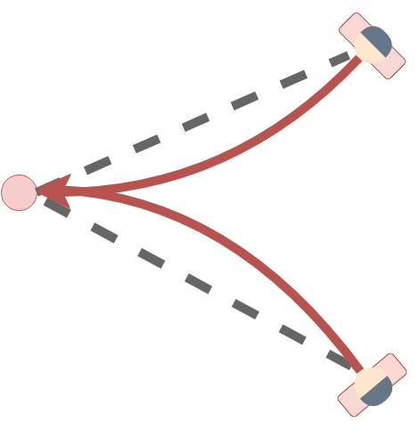
Figure 1: Two agents (e.g. pedestrians) move towards a goal (red circle). The dashed lines indicate the shortest path. Due to an interaction reward, the agents are incentivized to walk towards each other.

Quadratic Rewards: The following setup is useful for understanding the validity of the implementation of GS-CIOC and one of the differences to M-CIOC. We illustrate the scenario in figure 1: Two agents move towards a goal and are pulled together by an interaction reward, similar to people who belong together form a small group. We assume a cooperative reward function of the form $r=-\alpha_{1}(x_{1}^{2}+x_{2}^{2})-\alpha_{2}(u_{1}^{2}+u_{2}^{2})-\alpha_{3}(u_{1}+u_{2})^{2}$ (reward parameters, $\alpha_{i}\geq 0$, $x$-states, $u$-actions), i.e. both agents maximize the same reward. The dynamics are linear with $x_{t}=x_{t-1}+u_{t}$. We initialize one agent at $x=y=20$ and the other at $x=20,y=-20$. The reward function incentivizes both agents to move towards $x=y=0$. Though, they cannot do so in one step as non-zero actions are penalized quadratically. $-\alpha_{3}(u_{1}+u_{2})^{2}$ is special in that it induces an interaction of the agents. In particular, the term is maximized if $u_{1}=-u_{2}$. We roll-out 2000 trajectories over $T=14$ time-steps using M-CIOC and GS-CIOC. Figure 2 depicts the results. The mean solution of M-CIOC and GS-CIOC is practically identical, while the variances in the actions of each agent differ significantly.

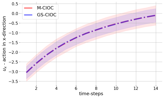
Figure 2: We illustrate the actions of an agent for the scenario described in figure 1. The reward setup is fully cooperative, i.e. both agents receive the same reward. Both M-CIOC and GS-CIOC can be applied to roll-out action sequences. Given 2000 roll-outs, the mean actions are in agreement between the two algorithms. Though, the standard deviation (shaded region) varies significantly. The reason for this is that agents can coordinate perfectly in M-CIOC. Therefore, one agent can compensate for larger deviations of the other agent from the mean and vice versa, leading to larger possible action amplitudes around the mean (they can minimize the interaction reward more effectively). GS-CIOC assumes uncoordinated execution of the action sequences, thus, exhibiting lower variance (interaction reward constricts movement around mean trajectory).

The reason for this is as follows. M-CIOC assumes agents that can coordinate their actions perfectly. This is not the case for GS-CIOC. While the deviations from the mean trajectory are almost decorrelated for GS-CIOC with a correlation coefficient of $-0.1$ (correlation between agent 1 and 2), those of M-CIOC are highly correlated with a correlation coefficient of $-0.7$. The variance resulting from M-CIOC algorithm is larger by a factor of $1.9$ than that for GS-CIOC. The reason is that if agent 1 chooses a specific action $\Delta u_{1}$ ($\Delta u_{1}$, deviation from mean trajectory/ expected action), then agent 2 can choose the action $\Delta u_{2}=-\Delta u_{1}$, canceling each other out in the interaction reward $-\alpha_{3}(u_{1}+u_{2})^{2}$. Through coordination, the agents experience a wider range of possible actions in M-CIOC. This is not necessarily a desirable property as we will demonstrate for the task of inferring the reward function.

To test how well the proposed algorithm can recover rewards from behaviour, we generate data trajectories based on a ground truth reward function. Given 2000 roll-outs of GS-CIOC we apply algorithm 6. We initialize the parameters at $\alpha=[1,1,1]$ and perform gradient ascent with a learning rate of $10^{-3}$ until the objective converges. The result is $\alpha_{1}=0.2(0.2)$, $\alpha_{2}=1.0(1.0)$, $\alpha_{3}=3.0(3.0)$. The values in the brackets indicate the true reward parameters. As we can see algorithm 6 recovered the rewards successfully.

What if we apply algorithm 6 to M-CIOC 2000 roll-outs? Again, we initialize the parameters at $\alpha=[1,1,1]$ and perform gradient ascent until convergence. We obtain: $\alpha_{1}=0.1(0.2)$, $\alpha_{2}=0.5(1.0)$, $\alpha_{3}=1.6(3.0)$. The inferred reward is almost half of the true reward, which matches the difference in observed variances of a factor of $1.9$. Depending on the application, either a reward inference algorithm based on M-CIOC or GS-CIOC will be more accurate (assuming fully cooperative reward functions). If a centralized controller controls the agents, then M-CIOC should be preferred, though, for decentralized controllers GS-CIOC is the better choice (i.e. algorithm 6).

We also tested the reward inference using different reward parameters with $\alpha_{1}=0.4(0.4)$, $\alpha_{2}=1.5(1.5)$, $\alpha_{3}=2.5(2.5)$ for one agent and $\alpha_{1}=0.2(0.2)$, $\alpha_{2}=1.0(1.0)$, $\alpha_{3}=3.0(3.0)$ for the other agent. Again, we were able to reproduce the parameter values using algorithm 6 (2000 trajectories, initialization at $\alpha=[1,1,1]$, GS-CIOC for roll-out and local policy approximation). In this case, M-CIOC cannot be used since it cannot handle different rewards per agent.

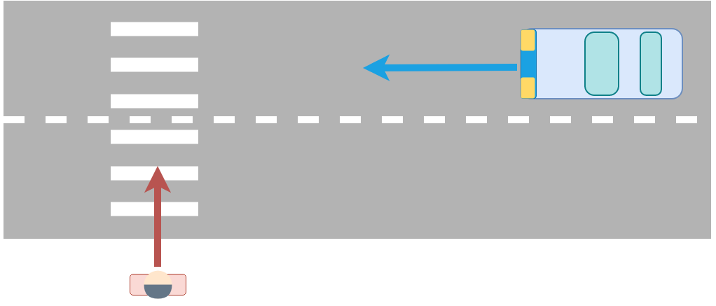
Figure 3: A pedestrian approaches a zebra crossing. The car will yield, though the pedestrian may be more or less socially inclined, speeding up so that the car can go on earlier or continue to walk at her most comfortable pace.

Traffic Interaction Scenario: A major advantage of GS-CIOC is the ease of defining reward functions for separate agents. Furthermore, in contrast to deterministic best responses, the maximum-entropy formulation is a form of reward-proportional error prediction, which was shown to capture human (boundedly-rational) behaviour well (Wright & Leyton-Brown, 2010). We demonstrate the interaction of a vehicle and a pedestrian at a zebra crossing in a simplified setting (see figure 3). We consider one case where the pedestrian also optimizes some of the reward of the vehicle (progress towards goal), i.e. the pedestrian is partially cooperative, vs the scenario where the pedestrian does not consider any of the vehicle’s reward. We implemented the iterative variant of the GS-CIOC algorithm. We roll-out 12 time-steps and initialize the trajectories with each agent standing still. Please refer to figure 4 for the results. The optimization takes 0.5s on a Titan Xp for a single trajectory and 0.6s for a batch of 100 trajectories, opening up the possibility of probing multiple initializations in real-time. For more details on the experiment (e.g. reward setup), please refer to the supplementary material.

The resulting behaviour varies significantly, underscoring the importance of being able to formulate reward functions on the continuum between full cooperation and no cooperation at all. In particular, the socially-minded pedestrian only considers a small part of the overall car specific reward function (namely, the goal reward). In a fully cooperative setup, both agents would be forced to share all of their rewards which complicates engineering a reward function that matches real-world behaviour.

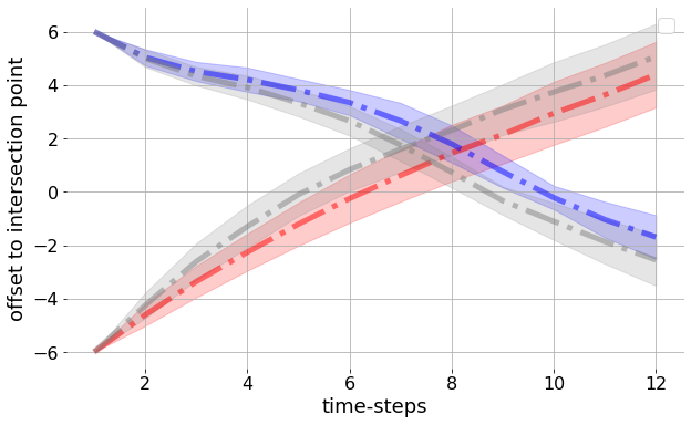
Figure 4: The pedestrian crosses the zebra crossing with an approaching car waiting until the pedestrian is on the other side (see also figure 3). The y-axis indicates the position relative to where the car and the pedestrian path intersect. The red (blue) curve corresponds to a pedestrian (car) that only considers her own reward. The grey curve corresponds to a pedestrian that values the progress of the car. Therefore, the latter speeds up in the beginning to make room for the car. The shaded regions indicate one standard deviation around the mean trajectory.

7 CONCLUSIONS

We presented a novel algorithm for predicting boundedly rational human behaviour in multi-agent stochastic games efficiently. Furthermore, the algorithm can be used to infer the rewards of those agents. We demonstrated its advantage for inferring rewards when agents execute their actions independently with limited communication. Also, we illustrated how diverse rewards affect the behaviour of agents and the variance inherent in maximum-entropy methods that model boundedly rational agents. We leave for future work the application to real-world traffic data.

8 SUPPLEMENTARY MATERIAL

ADDITIONAL BASELINES

We provide two additional baselines. One that compares the policy roll-outs of iterative GS-CIOC to those of a policy obtained from value iteration. The other checks how well the single-agent CIOC algorithm (Levine & Koltun, 2012) performs on multi-agent data.

Value Iteration Baseline

We will expand on the analysis in the experimental section of the main paper. Namely, we introduce a baseline to understand if iterative GS-CIOC finds a reasonable policy approximation. Figure 3 summarizes the toy example we consider. A pedestrian crosses the street, and an approaching car stops so that the pedestrian can cross safely.

The environment transitions are linear with $x_{kt}=x_{kt-1}+u_{kt}$. The reward setup is as follows. Both agents receive

• a quadratic lane keeping reward

• a quadratic velocity reward

• a quadratic goal reward

Additionally, the car receives an interaction reward of the form

$$\log(|x_{c}|+0.1)*\textnormal{sigmoid}(-x_{c}+6.)*\textnormal{sigmoid}(x_{c})\\ *\textnormal{sigmoid}(-y_{p})$$ (29)

where $x_{c}$ is the offset to the intersection point for the car in x-direction and $y_{p}$ is the offset to the intersection point for the pedestrian in y-direction. The pedestrian may also receive a reward for hurrying up while crossing. Namely, the pedestrian also receives the quadratic goal reward of the car on top of its own reward. We refer to that pedestrian as being socially minded.

We apply two methods to obtain a policy. The first method is iterative GS-CIOC, as described in the main paper. The second is value iteration using the soft-Bellman equation and a discretization of the state and action space. We perform value iteration for one agent at a time while the policy of the other agent is fixed, i.e. the policies are updated iteratively. These updates continue until the policies of both agents converge. We compare the policy roll-outs of both methods in figures 5 and 6.

Overall, the mean policy of iterative GS-CIOC converges close to the mean policy of the value iteration algorithm. Though, it gets stuck in local optima. Depending on the initial trajectories iterative GS-CIOC can slightly over- or under-shoot the value iteration reference trajectories. Figures 5 and 6 correspond to an initialization of both agents standing still at their respective starting positions (-6 and 6).

Apart from the mean policy roll-outs, the standard deviations show differences as well. Given only quadratic rewards, the iterative GS-CIOC standard deviation from the mean for the pedestrian (blue) in figure 5 agrees well with that of the value iteration algorithm. Though, the standard deviation is lower for the car (red) due to the non-quadratic nature of the interaction reward as GS-CIOC approximates the reward function with a second-order Taylor expansion. In other words, GS-CIOC may provide a biased estimate of the standard deviation.

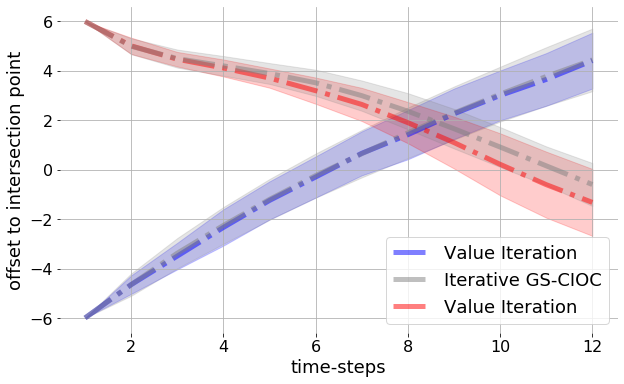
Figure 5: The pedestrian is not socially minded and crosses the zebra crossing without paying much attention to the car. The blue and red curves indicate a solution that we obtained from value iteration. The grey curves correspond to the solution of iterative GS-CIOC. Due to the localized nature of GS-CIOC, the mean trajectory does not match the solution of the value iteration perfectly. Given that GS-CIOC will consider the reward function up to a second-order Taylor expansion, the estimates of the standard deviation are not identical to those of the value iteration solution. The pedestrian only experiences quadratic rewards, while the car receives non-quadratic interaction rewards.

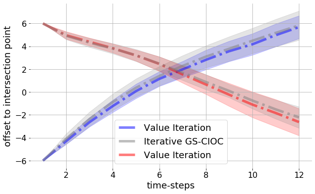
Figure 6: Same as figure 5, except here the pedestrian values the progress of the car, i.e. the pedestrian is more socially minded. The red and blue curves indicate the solution obtained from value iteration and the grey curves correspond to the solution of iterative GS-CIOC.

Single-Agent CIOC Baseline

Here we show which reward parameters CIOC infers given the ground-truth roll-outs of GS-CIOC in a non-cooperative reward setup. Since CIOC assumes a single agent setup, applying the algorithm to infer rewards for interacting agents corresponds to the assumption that other agents are non-reacting dynamic obstacles that follow pre-computed paths. We have already established that GS-CIOC produces the same mean trajectories as a multi-agent formulation of CIOC that we termed M-CIOC given cooperative rewards. The only difference was the resulting variance which we were able to explain in terms of the perfect coordination between agents for M-CIOC vs the decentralized execution in GS-CIOC.

The experimental setup is the same as that for the quadratic reward experiments in the main paper. Given 2000 roll-outs of GS-CIOC we apply CIOC to each agent. We repeat the procedure three times with varying seed values for the random number generators. The ranges of the reward parameters that we obtain are $\alpha=[0.245-0.248(0.40),1.017-1.043(1.50),1.945-1.954(2.50)]$ for one agent and $\alpha=[0.122-0.123(0.20),0.712-0.723(1.00),2.042-2.060(3.00)]$ for the other agent. The ground-truth reward parameters are indicated inside the brackets. CIOC cannot recover the correct rewards. In particular, the difference cannot be explained with a single reward scaling factor. The scaling factors would be $[0.613-0.619,0.678-0.696,0.778-0.782]$ for one agent and $[0.612-0.617,0.712-0.723,0.681-0.687]$ for the other agent. Therefore, the variation of the scaling factor is up to 20% in between the reward parameters of a single agent (e.g. 0.619 vs 0.778). This suggests that CIOC may incur a significant bias when estimating the reward parameters of interacting agents.

DERIVATION OF VALUE RECURSION FORMULAS

This section provides additional details on the derivation of the value recursion formulas in the methods section of the paper. Please read the methods section first. Also, our calculations follow a similar path like those in the supplementary material of (Levine & Koltun, 2012) for the single-agent case (LQR Likelihood Derivation, section B, Link).

Linearization of the Dynamics

$$\bar{x}_{kt} =A_{kt}\bar{x}_{kt-1}+B_{kt}\bar{u}_{kt}$$ (30)

$$A_{kt} =\frac{\partial\bar{x}_{kt}}{\partial\bar{x}_{kt-1}}$$ (31)

$$B_{kt} =\frac{\partial\bar{x}_{kt}}{\partial\bar{u}_{kt-1}}$$ (32)

Relevant Integrals

$$\int(\bar{u}_{jt}^{T}\phi_{u})\mathcal{N}(\mu_{jt};\Sigma_{jt})d\bar{u}_{jt}=\mu_{jt}^{T}\phi_{u}$$ (33)

$$\int\Big{(}\bar{x}_{jt}^{T}\phi_{x}\Big{)}\mathcal{N}(\mu_{jt};\Sigma_{jt})d\bar{u}_{jt}=\chi_{jt}^{T}\phi_{x}$$ (34)

$$\int(\bar{u}_{jt}^{T}\mathbf{\Phi_{u}}\bar{u}_{jt})\mathcal{N}(\mu_{jt};\Sigma_{jt})d\bar{u}_{jt}=\\ \mu_{jt}^{T}\mathbf{\Phi_{u}}\mu_{jt}+\sum_{nm}\Big{(}\mathbf{\Phi_{u}}\Big{)}_{nm}\Big{(}\Sigma_{jt}\Big{)}_{nm}$$ (35)

$$\int\Big{(}\bar{x}_{jt}^{T}\mathbf{\Phi_{x}}\bar{x}_{jt}\Big{)}\mathcal{N}(\mu_{jt};\Sigma_{jt})d\bar{u}_{jt}=\\ \chi_{jt}^{T}\mathbf{\Phi_{x}}\chi_{jt}+\sum_{nm}\Big{(}B_{jt}^{T}\mathbf{\Phi_{x}}B_{jt}\Big{)}_{nm}\Big{(}\Sigma_{jt}\Big{)}_{nm}$$ (36)

where

$$\chi_{jt}=A_{jt}\bar{x}_{jt-1}+B_{jt}\mu_{jt}$$ (37)

is the mean state that agent $j$ transitions to.

Quadratic Reward Approximation

In contrast to (Levine & Koltun, 2012), we will also consider reward terms where states and actions mix. The full second-order Taylor expansion of the reward is given by

$$r(\bar{x}_{it},\bar{x}_{jt},\bar{u}_{it},\bar{u}_{jt})\approx\\ r_{t}+\begin{bmatrix}\bar{x}_{it}\\ \bar{x}_{jt}\\ \bar{u}_{it}\\ \bar{u}_{jt}\end{bmatrix}^{T}H_{t}\begin{bmatrix}\bar{x}_{it}\\ \bar{x}_{jt}\\ \bar{u}_{it}\\ \bar{u}_{jt}\end{bmatrix}+\begin{bmatrix}\bar{x}_{it}\\ \bar{x}_{jt}\\ \bar{u}_{it}\\ \bar{u}_{jt}\end{bmatrix}^{T}g_{t}\\ =r_{t}+\bar{x}_{jt}^{T}\Big{(}H_{(x_{j}x_{i})t}\bar{x}_{it}\Big{)}+\bar{u}^{T}_{jt}\Big{(}H_{(u_{j}u_{i})t}\bar{u}_{it}\Big{)}\\ +\bar{u}_{it}^{T}\Big{(}H_{(u_{i}x_{j})t}\bar{x}_{jt}\Big{)}+\bar{u}_{jt}^{T}\Big{(}H_{(u_{j}x_{i})t}\bar{x}_{it}\Big{)}\\ +\sum_{k\in\{i,j\}}\Bigg{[}\bar{x}_{kt}^{T}\Big{(}\frac{1}{2}H_{(x_{k}x_{k})t}\Big{)}\bar{x}_{kt}+\bar{u}^{T}_{kt}\Big{(}\frac{1}{2}H_{(u_{k}u_{k})t}\Big{)}\bar{u}_{kt}\\ +\bar{u}_{kt}^{T}g_{u_{k}t}+\bar{x}_{kt}^{T}g_{x_{k}t}\Bigg{]}$$ (38)

$$H_{(x_{n}x_{m})t} =\frac{\partial^{2}r}{\partial\bar{x}_{nt}\partial\bar{x}_{mt}}$$ (39)

$$H_{(u_{n}u_{m})t} =\frac{\partial^{2}r}{\partial\bar{u}_{nt}\partial\bar{u}_{mt}}$$ (40)

$$H_{(u_{n}x_{m})t} =\frac{\partial^{2}r}{\partial\bar{u}_{nt}\partial\bar{x}_{mt}}$$ (41)

$$g_{x_{n}t} =\frac{\partial r}{\partial\bar{x}_{nt}}$$ (42)

$$g_{u_{n}t} =\frac{\partial r}{\partial\bar{u}_{nt}}$$ (43)

We assume that the derivatives commute, i.e.

$$H_{(u_{m}x_{n})t}^{T}=H_{(x_{n}u_{m})t}$$ (44)

We can expand some of the $\bar{x}_{kt}$ using the linearization of the dynamics in (30). This allows us to introduce a few convenient re-definitions of the Hessian matrices and gradients which we will use for the remainder of the derivation.

$$\tilde{H}_{(ji)t} =B_{jt}^{T}H^{T}_{(u_{i}x_{j})t}+H_{(u_{j}x_{i})t}B_{it}+H_{(u_{j}u_{i})t}$$ (45)

$$\tilde{H}_{(ii)t} =\frac{1}{2}\Big{(}H_{(u_{i}x_{i})t}B_{it}+B_{it}^{T}H_{(u_{i}x_{i})t}^{T}\Big{)}+H_{(u_{i}u_{i})t}$$ (46)

$$\tilde{H}_{(jj)t} =\frac{1}{2}\Big{(}H_{(u_{j}x_{j})t}B_{jt}+B_{jt}^{T}H_{(u_{j}x_{j})t}^{T}\Big{)}+H_{(u_{j}u_{j})t}$$ (47)

$$\hat{H}_{(nm)t} =H_{(x_{n}x_{m})t}$$ (48)

$$\tilde{g}_{it} =g_{u_{i}t}+H_{(u_{i}x_{i})t}A_{it}\bar{x}_{it-1}+H_{(u_{i}x_{j})t}A_{jt}\bar{x}_{jt-1}$$ (49)

$$\tilde{g}_{jt} =g_{u_{j}t}+H_{(u_{j}x_{j})t}A_{jt}\bar{x}_{jt-1}+H_{(u_{j}x_{i})t}A_{it}\bar{x}_{it-1}$$ (50)

$$\hat{g}_{nt} =g_{x_{n}t}$$ (51)

The reward approximation given the re-defined Hessians and gradients is as follows.

$$r(\bar{x}_{it},\bar{x}_{jt},\bar{u}_{it},\bar{u}_{jt})\approx\\ r_{t}+\bar{x}_{jt}^{T}\Big{(}\hat{H}_{(ji)t}\bar{x}_{it}\Big{)}+\bar{u}^{T}_{jt}\Big{(}\tilde{H}_{(ji)t}\bar{u}_{it}\Big{)}\\ +\sum_{k\in\{i,j\}}^{2}\Bigg{[}\bar{x}_{kt}^{T}\Big{(}\frac{1}{2}\hat{H}_{(kk)t}\Big{)}\bar{x}_{kt}+\bar{u}^{T}_{kt}\Big{(}\frac{1}{2}\tilde{H}_{(kk)t}\Big{)}\bar{u}_{kt}+\\ \bar{u}_{kt}^{T}\tilde{g}_{kt}+\bar{x}_{kt}^{T}\hat{g}_{kt}\Bigg{]}$$ (52)

As we have seen in the methods section, the value function will be quadratic in the states given the reward approximation.

$$V_{it+1}(\bar{x}_{1t},\bar{x}_{2t})=\bar{x}^{T}_{jt}\Big{(}\hat{V}_{(ji)t}\bar{x}_{it}\Big{)}+\\ \sum_{k=1}^{2}\left[\bar{x}^{T}_{kt}\Big{(}\frac{1}{2}\hat{V}_{(kk)t}\Big{)}\bar{x}_{kt}+\bar{x}^{T}_{kt}\hat{v}_{kt}\right]+c$$ (53)

$$\hat{V}_{(nm)t} =\frac{\partial^{2}r}{\partial\bar{x}_{nt}\partial\bar{x}_{mt}}$$ (54)

$$\hat{v}_{nt} =\frac{\partial r}{\partial\bar{x}_{nt}}$$ (55)

The constant $c$ in the value function is going to be irrelevant (does not affect policy) and will be dropped from now on.

Q-function

$$Q_{it}(\bar{x}_{it-1},\bar{x}_{jt-1},\bar{u}_{it})=\\ \int p(\bar{x}_{it},\bar{x}_{jt}|\bar{x}_{it-1},\bar{x}_{jt-1},\bar{u}_{it},\bar{u}_{jt})\pi_{jt}(\bar{u}_{jt}|\bar{x}_{it-1},\bar{x}_{jt-1})\\ \Big{(}r(\bar{x}_{it},\bar{x}_{jt},\bar{u}_{it},\bar{u}_{jt})+V_{it+1}(\bar{x}_{it},\bar{x}_{jt})\Big{)}d\bar{u}_{jt}d\bar{x}_{it}d\bar{x}_{jt}$$ (57)

As we have argued in the methods section, the policy $\pi_{jt}$ is a Gaussian policy of the form $\pi_{jt}\sim\exp\left(-\frac{1}{2}(\bar{u}_{jt}-\mu_{jt})^{T}\Sigma_{jt}^{-1}(\bar{u}_{jt}-\mu_{jt})\right)$. Substituting 52 and 53 in 57 results in quite a few terms of the type 33-36 and trivial terms (simple Gaussian integral).

We collect the terms so that they resemble the integrals in 33-36 and define

$$\Phi_{x}=\frac{1}{2}\hat{V}_{(jj)t}+\frac{1}{2}\hat{H}_{(jj)t}$$ (58)

$$\phi_{x}=\hat{H}_{(ji)t}\bar{x}_{it}+\hat{V}_{(ji)t}\bar{x}_{it}+\hat{g}_{jt}+\hat{v}_{jt}$$ (59)

for the terms where $\bar{x}_{jt}$ needs to be integrated over and

$$\Phi_{u}=\frac{1}{2}\tilde{H}_{(jj)t}$$ (60)

$$\phi_{u}=\tilde{H}_{(ji)t}\bar{u}_{it}+\tilde{g}_{jt}$$ (61)

for those with $\bar{u}_{jt}$ as the integration variable.

After integration and dropping a few irrelevant constants (no state or action dependencies) we get the following Q-function.

$$Q_{it}(\bar{x}_{1t-1},\bar{x}_{2t-1},\bar{u}_{it})=g(\bar{x}_{it},\bar{u}_{it})+\chi_{jt}^{T}\Phi_{x}\chi_{jt}\\ \mu^{T}_{jt}\Phi_{u}\mu_{jt}+\chi_{jt}^{T}\phi_{x}(\bar{x}_{it})+\mu_{jt}^{T}\phi_{u}(\bar{u}_{it})$$ (62)

where

$$g(\bar{x}_{it},\bar{u}_{it})=\bar{x}_{it}^{T}\Big{(}\frac{1}{2}\hat{H}_{(ii)t}\Big{)}\bar{x}_{it}+\bar{u}^{T}_{it}\Big{(}\frac{1}{2}\tilde{H}_{(ii)t}\Big{)}\bar{u}_{it}+\\ \bar{u}_{it}^{T}\tilde{g}_{it}+\bar{x}_{it}^{T}\hat{g}_{it}+\bar{x}^{T}_{it}\Big{(}\frac{1}{2}\hat{V}_{(ii)t}\Big{)}\bar{x}_{it}+\bar{x}^{T}_{it}\hat{v}_{it}$$ (63)

Value Function

To derive the value recursion for the decentralized setting, we rearrange the values in the Q-function so that it resembles the single-agent version. The integration $V_{it}=\log\int\exp(Q_{it}(\bar{u}_{it}))d\bar{u}_{it}$ that provides us with the value function at time-step $t$ is then the same as that of the single agent case. We give the single-agent result as a reference (taken from supplementary material of (Levine & Koltun, 2012)).

  Single agent reference solution of (Levine & Koltun, 2012).

$$Q_{t}( \bar{x}_{t-1},\bar{u}_{t})=\frac{1}{2}\bar{u}_{t}^{T}\tilde{H}_{t}\bar{u}_{t}+\bar{u}_{t}^{T}\tilde{g}_{t}$$ (64)

$$+\frac{1}{2}\underbrace{[A_{t}\bar{x}_{t-1}+B_{t}\bar{u}_{t}]}_{\bar{x}_{t}}^{T}\underbrace{\Big{[}\hat{H}_{t}+\hat{V}_{t}\Big{]}}_{\hat{Q}_{t}}[A_{t}\bar{x}_{t-1}+B_{t}\bar{u}_{t}]$$ (65)

$$+[A_{t}\bar{x}_{t-1}+B_{t}\bar{u}_{t}]^{T}\underbrace{[\hat{g}_{t}+\hat{v}_{t}]}_{\hat{q}_{t}}$$ (66)

The resulting value function $V_{t}=\log\int\exp(Q_{t}(\bar{u}_{t}))d\bar{u}_{t}$ is

$$V_{t}(\bar{x}_{t-1}) =\frac{1}{2}\bar{x}_{t-1}^{T}A_{t}^{T}\hat{Q}_{t}A_{t}\bar{x}_{t-1}+\bar{x}_{t-1}^{T}A_{t}^{T}\hat{q}_{t}$$ (67)

$$-\frac{1}{2}\tilde{\mu}_{t}^{T}\tilde{M}_{t}\tilde{\mu}_{t}-\frac{1}{2}\log|-\tilde{M}_{t}|$$ (68)

with

$$\tilde{\mu}_{t} =\tilde{M}_{t}^{-1}\Big{(}\tilde{g}_{t}+B_{t}^{T}\hat{q}_{t}+B_{t}^{T}\hat{Q}_{t}A_{t}\bar{x}_{t-1})$$ (69)

$$\tilde{M}_{t} =\tilde{H}_{t}+B_{t}^{T}\hat{Q}_{t}B_{t}$$ (70)

 

We use the single-agent solution as a template for the two-agent derivation of the value function given the Q-function.

$$Q_{it}(\bar{x}_{1t-1},\bar{x}_{2t-1},\bar{u}_{it})=\\ \frac{1}{2}\bar{x}_{it}^{T}\hat{Q}_{it}\bar{x}_{it}+\frac{1}{2}\bar{u}_{it}^{T}\tilde{H}_{(ii)t}\bar{u}_{it}+\bar{u}_{it}\tilde{g}_{ijt}^{*}+\bar{x}_{it}^{T}\hat{q}_{ijt}+C_{jt}$$ (71)

with

$$\hat{Q}_{it}=\hat{H}_{(ii)t}+\hat{V}_{(ii)t}$$ (72)

$$\tilde{g}_{ijt}^{*}=\tilde{g}_{it}+\tilde{H}_{(ij)t}\mu_{jt}$$ (73)

$$\hat{q}_{ijt}=\hat{g}_{it}+\hat{v}_{it}+\hat{H}_{(ij)t}\chi_{jt}+\hat{V}_{(ij)t}\chi_{jt}$$ (74)

$$C_{jt}=\chi_{jt}^{T}\Phi_{x}\chi_{jt}+\mu^{T}_{jt}\Phi_{u}\mu_{jt}+\chi_{jt}^{T}[\hat{g}_{jt}+\hat{v}_{jt}]+\mu_{jt}^{T}\tilde{g}_{jt}$$ (75)

$$C_{jt}=\frac{1}{2}\bar{x}_{jt-1}^{T}A^{T}_{jt}\hat{Q}_{jt}A_{jt}\bar{x}_{jt-1}+\frac{1}{2}\mu^{T}_{jt}\tilde{M}_{jt}\mu_{jt}+\\ \bar{x}_{jt-1}^{T}A^{T}_{jt}\hat{Q}_{jt}B_{jt}\mu_{jt}+\chi_{jt}^{T}[\hat{g}_{jt}+\hat{v}_{jt}]+\mu_{jt}^{T}\tilde{g}_{jt}$$ (76)

The value function for timestep $t$ is

$$V_{it}(\bar{x}_{it-1},\bar{x}_{jt-1})=\frac{1}{2}\bar{x}_{it-1}^{T}A^{T}_{it}\hat{Q}_{it}A_{it}\bar{x}_{it-1}+\\ \bar{x}_{it-1}^{T}A_{it}^{T}\hat{q}_{ijt}-\frac{1}{2}\mu_{it}^{T}\tilde{M}_{it}\mu_{it}-\frac{1}{2}\log|-\tilde{M}_{it}|+C_{jt}$$ (77)

$$\mu_{it}=-\tilde{M}^{-1}_{it}\Big{(}\tilde{g}_{ijt}^{*}+B^{T}_{it}\hat{q}_{ijt}+B^{T}_{it}\hat{Q}_{it}A_{it}\bar{x}_{it-1}\Big{)}$$ (78)

$$\tilde{M}_{it}=\tilde{H}_{(ii)t}+B^{T}_{it}\hat{Q}_{it}B_{it}$$ (79)

$\mu_{it}$ corresponds to the expected action of agent i considering the interaction effects with agent j. $\tilde{M}_{it}$ is the precision matrix that corresponds to the actions of agent i. Therefore, the solution resembles the single agent case.

Deriving Mean

We expand (78) by substituting the definitions of $\tilde{g}^{*}$, $\tilde{g}$, $\hat{q}$ and $\chi$. The result is a linear equation in the mean actions $\mu_{mt}$.

$$-\boldsymbol{\mu}_{it}= \tilde{M}_{it}^{-1}\Big{[}\tilde{g}_{it}+B_{it}^{T}\hat{q}_{it}\Big{]}+\tilde{M}_{it}^{-1}B_{it}^{T}\hat{Q}_{it}A_{it}\bar{x}_{it-1}$$

$$+ \tilde{M}^{-1}_{it}B_{it}\hat{Q}_{(ij)t}A_{jt}\bar{x}_{jt-1}+\tilde{M}^{-1}_{it}\tilde{M}_{(ij)t}\boldsymbol{\mu}_{jt}$$

$$= \tilde{M}_{it}^{-1}\Big{(}\alpha_{i}^{(i)}+\beta_{i}^{(i)}\bar{x}_{it-1}+\gamma_{ij}^{(i)}\bar{x}_{jt-1}+\delta_{ij}^{(i)}\boldsymbol{\mu}_{jt}\Big{)}$$ (80)

$$\Rightarrow \Big{[}\delta_{ij}^{(i)}\Big{(}\tilde{M}_{jt}^{-1}\Big{)}^{(j)}\delta_{ji}^{(j)}-\Big{(}\tilde{M}_{it}\Big{)}^{(i)}\Big{]}\mu_{it}=$$

$$\alpha_{i}^{(i)}-\delta_{ij}^{(i)}\Big{(}\tilde{M}_{jt}^{-1}\Big{)}^{(j)}\alpha_{j}^{(j)}+$$

$$\Big{(}\beta_{i}^{(i)}-\delta_{ij}^{(i)}\Big{(}\tilde{M}_{jt}^{-1}\Big{)}^{(j)}\gamma_{ji}^{(j)}\Big{)}\bar{x}_{it-1}+$$

$$\Big{(}\gamma_{ij}^{(i)}-\delta_{ij}^{(i)}\Big{(}\tilde{M}_{jt}^{-1}\Big{)}^{(j)}\beta_{j}^{(j)}\Big{)}\bar{x}_{jt-1}$$ (81)

with

$$\alpha_{i}^{(i)}= \Big{[}g_{u_{i}t}+B_{it}^{T}\hat{q}_{it}\Big{]}$$ (82)

$$\beta_{i}^{(i)}= \hat{Q}_{it}^{\dagger}A_{it}$$ (83)

$$\gamma_{ij}^{(i)}= \hat{Q}_{(ij)t}^{\dagger}A_{jt}$$ (84)

$$\delta_{ij}^{(i)}= \tilde{M}_{(ij)t}$$ (85)

$$\hat{Q}^{\dagger}_{(mn)t}= H_{u_{m}x_{n}}+B^{T}_{mt}\hat{Q}_{(mn)t}$$ (86)

The ⁽ⁱ⁾ index indicates which agent the derivatives/ value functions refer to. We indicate the index on the left side of the above equations but drop it otherwise for brevity.

Value Recursion Formulas

Now that we understand what the Q-function and the policy look like, we determine the set of recursive equations that provide us with the value function matrices at timestep $t$.

$$V_{it}( \bar{x}_{it-1},\bar{x}_{jt-1})={\color[rgb]{0,0,1}\Bigg{[}}\frac{1}{2}\bar{x}_{it-1}^{T}A^{T}_{it}\hat{Q}_{it}A_{it}\bar{x}_{it-1}$$

$$+\bar{x}_{it-1}^{T}A_{it}^{T}\hat{q}_{it}-\frac{1}{2}\bar{\mu}_{it}^{T}\tilde{M}_{it}\bar{\mu}_{it}-\frac{1}{2}\log|-\tilde{M}_{it}|$$

$$-\frac{1}{2}\mu_{it}^{*T}\tilde{M}_{it}\mu_{it}^{*}-\bar{\mu}_{it}^{T}\tilde{M}_{it}\mu_{it}^{*}{\color[rgb]{0,0,1}\Bigg{]}_{\textnormal{single agent}}}$$

$$+{\color[rgb]{1,0,0}\Bigg{[}}\frac{1}{2}\chi_{jt}^{T}D_{\chi\chi}\chi_{jt}+\frac{1}{2}\mu_{jt}^{T}D_{\mu\mu}\mu_{jt}+\mu_{jt}^{T}D_{\mu\chi}\chi_{jt}$$

$$+\mu_{jt}^{T}D_{\mu x}\bar{x}_{it-1}+\chi_{jt}^{T}D_{\chi x}\bar{x}_{it-1}+\mu_{jt}^{T}D_{\mu}$$

$$+\mu_{jt}^{T}D^{*}_{\mu}+\chi_{jt}^{T}D_{\chi}+\chi_{jt}^{T}D^{*}_{\chi}{\color[rgb]{1,0,0}\Bigg{]}_{\textnormal{interaction}}}$$ (87)

$$\bar{\mu}_{it}= -\tilde{M}^{-1}_{it}\Big{(}g_{u_{i}t}+B^{T}_{it}\hat{q}_{it}+B^{T}_{it}\hat{Q}_{it}A_{it}\bar{x}_{it-1}\Big{)}$$ (88)

$$\mu_{it}^{*}= -\tilde{M}_{it}^{-1}\Big{(}H_{u_{i}x_{i}}A_{i}x_{it-1}+H_{u_{i}x_{j}}A_{j}x_{jt-1}\Big{)}$$ (89)

$$D_{\chi\chi}=\hat{Q}_{(jj)t}-\hat{Q}_{(ji)t}B_{it}\tilde{M}_{it}^{-1}B_{it}^{T}\hat{Q}_{(ij)t}$$ (90)

$$D_{\mu\mu}=\tilde{H}_{(jj)t}-\tilde{H}_{(ji)t}\tilde{M}_{it}^{-1}\tilde{H}_{(ij)t}$$ (91)

$$D_{\mu\chi}=-\tilde{H}_{(ji)t}\tilde{M}_{it}^{-1}B^{T}_{it}\hat{Q}_{(ij)t}$$ (92)

$$D_{\mu x}=-\tilde{H}_{(ji)t}\tilde{M}^{-1}_{it}B_{it}^{T}\hat{Q}_{it}A_{it}$$ (93)

$$D_{\chi x}=\hat{Q}_{(ji)t}A_{it}-\hat{Q}_{(ji)t}B_{it}\tilde{M}^{-1}_{it}B^{T}_{it}\hat{Q}_{it}A_{it}$$ (94)

$$D_{\mu}=g_{u_{j}t}-\tilde{H}_{(ji)t}\tilde{M}^{-1}_{it}[g_{u_{i}t}+B_{it}^{T}\hat{q}_{it}]$$ (95)

$$D^{*}_{\mu} =H_{(u_{j}x_{i})t}A_{it}\bar{x}_{it-1}+H_{(u_{j}x_{j})t}A_{jt}\bar{x}_{jt-1}$$

$$-\tilde{H}_{(ji)t}\tilde{M}^{-1}_{it}\Big{[}H_{(u_{i}x_{i})t}A_{it}\bar{x}_{it-1}+H_{(u_{i}x_{j})t}A_{jt}\bar{x}_{jt-1}\Big{]}$$ (96)

$$D_{\chi}=\hat{g}_{jt}+\hat{v}_{jt}-\hat{Q}_{(ji)t}B_{it}\tilde{M}^{-1}_{it}[\tilde{g}_{it}+B^{T}_{it}\hat{q}_{it}]$$ (97)

$$D^{*}_{\chi} =-\hat{Q}_{(ji)t}B_{it}\tilde{M}^{-1}_{it}\Big{[}H_{(u_{i}x_{i})t}A_{it}\bar{x}_{it-1}$$

$$+H_{(u_{i}x_{j})t}A_{jt}\bar{x}_{jt-1}\Big{]}$$ (98)

$\mu_{it}^{*}$, $D_{\mu}^{*}$ and $D_{\chi}^{*}$ are correction terms due to the mixing of states and actions in the reward function.

In the next step, we collect all the $\bar{x}_{kt-1}$ terms to reconstruct the value function at $t$. In order to do so we need to consider the state dependency of $\mu$ which did not play any role so far as it depends only on the states at $t-1$ and not $t$.

$$\mu_{jt}=\nu_{jt}+\Pi_{jt}\bar{x}_{it-1}+\Omega_{jt}\bar{x}_{jt-1}$$ (99)

$$-\frac{1}{2}\mu_{it}^{*T} \tilde{M}_{it}\mu_{it}^{*}-\bar{\mu}_{it}^{T}\tilde{M}_{it}\mu^{*}_{it}=$$

$$-{\color[rgb]{0,0,1}\bar{x}_{it-1}^{T}}A_{it}^{T}H_{x_{i}u_{i}}\tilde{M}_{it}^{-1}\Big{(}g_{u_{it}}+B_{it}^{T}\hat{q}_{it}\Big{)}$$

$$-{\color[rgb]{1,0,0}\bar{x}_{jt-1}^{T}}A_{jt}^{T}H_{x_{j}u_{i}}\tilde{M}_{it}^{-1}\Big{(}g_{u_{it}}+B_{it}^{T}\hat{q}_{it}\Big{)}$$

$$-{\color[rgb]{0,0,1}\bar{x}_{it-1}^{T}}A_{it}^{T}\hat{Q}_{it}B_{it}\tilde{M}_{it}^{-1}H_{u_{i}x_{i}}A_{it}{\color[rgb]{0,0,1}\bar{x}_{it-1}}$$

$$-{\color[rgb]{1,0,0}\bar{x}_{jt-1}^{T}}A_{jt}^{T}H_{x_{j}u_{i}}\tilde{M}_{it}^{-1}B_{it}^{T}\hat{Q}_{it}A_{it}{\color[rgb]{0,0,1}\bar{x}_{it-1}}$$

$$-{\color[rgb]{1,0,0}\bar{x}_{jt-1}^{T}}A_{jt}^{T}H_{x_{j}u_{i}}\tilde{M}_{it}^{-1}H_{u_{i}x_{i}}A_{it}{\color[rgb]{0,0,1}\bar{x}_{it-1}}$$

$$-\frac{1}{2}{\color[rgb]{1,0,0}\bar{x}_{jt-1}^{T}}A_{jt}^{T}H_{x_{j}u_{i}}\tilde{M}_{it}^{-1}H_{u_{i}x_{j}}A_{jt}{\color[rgb]{1,0,0}\bar{x}_{jt-1}}$$

$$-\frac{1}{2}{\color[rgb]{0,0,1}\bar{x}_{it-1}^{T}}A_{it}^{T}H_{x_{i}u_{i}}\tilde{M}_{it}^{-1}H_{u_{i}x_{i}}A_{it}{\color[rgb]{0,0,1}\bar{x}_{it-1}}$$ (100)

$$\frac{1}{2}\chi_{jt}^{T}D_{\chi\chi}\chi_{jt}= \frac{1}{2}{\color[rgb]{1,0,0}\bar{x}_{jt-1}^{T}}(A_{jt}+B_{jt}\Omega_{jt})^{T}D_{\chi\chi}(A_{jt}+B_{jt}\Omega_{jt}){\color[rgb]{1,0,0}\bar{x}_{jt-1}}$$

$$+\frac{1}{2}{\color[rgb]{0,0,1}\bar{x}_{it-1}^{T}}\Pi_{jt}^{T}B^{T}_{jt}D_{\chi\chi}B_{jt}\Pi_{jt}{\color[rgb]{0,0,1}\bar{x}_{it-1}}$$

$$+{\color[rgb]{1,0,0}\bar{x}_{jt-1}^{T}}(A_{jt}+B_{jt}\Omega_{jt})^{T}D_{\chi\chi}B_{jt}\Pi_{jt}{\color[rgb]{0,0,1}\bar{x}_{it-1}}$$

$$+{\color[rgb]{1,0,0}\bar{x}_{jt-1}^{T}}(A_{jt}+B_{jt}\Omega_{jt})^{T}D_{\chi\chi}B_{jt}\nu_{jt}$$

$$+{\color[rgb]{0,0,1}\bar{x}_{it-1}^{T}}\Pi_{jt}^{T}B_{jt}^{T}D_{\chi\chi}B_{jt}\nu_{jt}+const$$ (101)

$$\frac{1}{2}\mu_{jt}^{T}D_{\mu\mu}\mu_{jt}= \frac{1}{2}{\color[rgb]{1,0,0}\bar{x}_{jt-1}^{T}}\Omega_{jt}^{T}D_{\mu\mu}\Omega_{jt}{\color[rgb]{1,0,0}\bar{x}_{jt-1}}$$

$$+\frac{1}{2}{\color[rgb]{0,0,1}\bar{x}_{it-1}^{T}}\Pi_{jt}^{T}D_{\mu\mu}\Pi_{jt}{\color[rgb]{0,0,1}\bar{x}_{it-1}}$$

$$+{\color[rgb]{1,0,0}\bar{x}_{jt-1}^{T}}\Omega_{jt}^{T}D_{\mu\mu}\Pi_{jt}{\color[rgb]{0,0,1}\bar{x}_{it-1}}$$

$$+{\color[rgb]{1,0,0}\bar{x}_{jt-1}^{T}}\Omega_{jt}^{T}D_{\mu\mu}\nu_{jt}$$

$$+{\color[rgb]{0,0,1}\bar{x}_{it-1}^{T}}\Pi_{jt}^{T}D_{\mu\mu}\nu_{jt}+const$$ (102)

$$\mu_{jt}^{T}D_{\mu\chi}\chi_{jt} =\Big{[}{\color[rgb]{1,0,0}\bar{x}_{jt-1}^{T}}A_{jt}^{T}D_{\mu\chi}^{T}\nu_{jt}$$

$$+{\color[rgb]{1,0,0}\bar{x}_{jt-1}^{T}}A_{jt}^{T}D_{\mu\chi}^{T}\Pi_{jt}{\color[rgb]{0,0,1}\bar{x}_{it-1}}$$

$$+{\color[rgb]{1,0,0}\bar{x}_{jt-1}^{T}}A_{jt}^{T}D_{\mu\chi}^{T}\Omega_{jt}{\color[rgb]{1,0,0}\bar{x}_{jt-1}}\Big{]}$$

$$+\Big{[}{\color[rgb]{1,0,0}\bar{x}_{jt-1}^{T}}\Omega_{jt}^{T}(D_{\mu\chi}B_{jt})\Omega_{jt}{\color[rgb]{1,0,0}\bar{x}_{jt-1}}$$

$$+{\color[rgb]{0,0,1}\bar{x}_{it-1}^{T}}\Pi_{jt}^{T}(D_{\mu\chi}B_{jt})\Pi_{jt}{\color[rgb]{0,0,1}\bar{x}_{it-1}}$$

$$+{\color[rgb]{1,0,0}\bar{x}_{jt-1}^{T}}\Omega_{jt}^{T}(D_{\mu\chi}B_{jt}+B_{jt}^{T}D_{\mu\chi}^{T})\Pi_{jt}{\color[rgb]{0,0,1}\bar{x}_{it-1}}$$

$$+{\color[rgb]{1,0,0}\bar{x}_{jt-1}^{T}}\Omega_{jt}^{T}(D_{\mu\chi}B_{jt}+B_{jt}^{T}D_{\mu\chi}^{T})\nu_{jt}$$

$$+{\color[rgb]{0,0,1}\bar{x}_{it-1}^{T}}\Pi_{jt}^{T}(D_{\mu\chi}B_{jt}+B_{jt}^{T}D_{\mu\chi}^{T})\nu_{jt}\Big{]}+const$$ (103)

$$\mu_{jt}^{T}D_{\mu x}\bar{x}_{it-1}= {\color[rgb]{0,0,1}\bar{x}_{it-1}^{T}}D_{\mu x}^{T}\nu_{jt}+{\color[rgb]{0,0,1}\bar{x}_{it-1}^{T}}D_{\mu x}^{T}\Pi_{jt}{\color[rgb]{0,0,1}\bar{x}_{it-1}}$$

$$+{\color[rgb]{1,0,0}\bar{x}_{jt-1}^{T}}\Omega_{jt}^{T}D_{\mu x}{\color[rgb]{0,0,1}\bar{x}_{it-1}}$$ (104)

$$\chi_{jt}^{T}D_{\chi x}\bar{x}_{it-1} ={\color[rgb]{1,0,0}\bar{x}_{jt-1}^{T}}A_{jt}^{T}D_{\chi x}{\color[rgb]{0,0,1}\bar{x}_{it-1}}$$

$$+{\color[rgb]{0,0,1}\bar{x}_{it-1}^{T}}(D_{\chi x}^{T}B_{jt})\nu_{jt}$$

$$+{\color[rgb]{0,0,1}\bar{x}_{it-1}^{T}}(D_{\chi x}^{T}B_{jt})\Pi_{jt}{\color[rgb]{0,0,1}\bar{x}_{it-1}}$$

$$+{\color[rgb]{1,0,0}\bar{x}_{jt-1}^{T}}\Omega_{jt}^{T}(B_{jt}^{T}D_{\chi x}){\color[rgb]{0,0,1}\bar{x}_{it-1}}$$ (105)

$$\mu_{jt}^{T}D_{\mu}= {\color[rgb]{0,0,1}\bar{x}_{it-1}^{T}}\Pi_{jt}^{T}D_{\mu}+{\color[rgb]{1,0,0}\bar{x}_{jt-1}^{T}}\Omega_{jt}^{T}D_{\mu}+const$$ (106)

$$\chi_{jt}^{T}D_{\chi}= {\color[rgb]{1,0,0}\bar{x}_{jt-1}^{T}}A_{jt}^{T}D_{\chi}$$

$$+{\color[rgb]{0,0,1}\bar{x}_{it-1}^{T}}\Pi_{jt}^{T}(B_{jt}^{T}D_{\chi})+{\color[rgb]{1,0,0}\bar{x}_{jt-1}^{T}}\Omega_{jt}^{T}(B_{jt}^{T}D_{\chi})$$

$$+const$$ (107)

$$\mu_{jt}^{T}D^{*}_{\mu} ={\color[rgb]{0,0,1}\bar{x}_{it-1}^{T}}A_{it}^{T}\Big{(}H_{x_{i}u_{j}}-H_{x_{i}u_{i}}\tilde{M}_{it}^{-1}\tilde{H}_{(ij)t}\Big{)}\nu_{jt}$$

$$+{\color[rgb]{1,0,0}\bar{x}_{jt-1}^{T}}A_{jt}^{T}\Big{(}H_{x_{j}u_{j}}-H_{x_{j}u_{i}}\tilde{M}_{it}^{-1}\tilde{H}_{(ij)t}\Big{)}\nu_{jt}$$

$$+{\color[rgb]{0,0,1}\bar{x}_{it-1}^{T}}\Pi_{jt}^{T}\Big{(}H_{u_{j}x_{i}}-\tilde{H}_{(ji)t}\tilde{M}_{it}^{-1}H_{u_{i}x_{i}}\Big{)}A_{it}{\color[rgb]{0,0,1}\bar{x}_{it-1}}$$

$$+{\color[rgb]{0,0,1}\bar{x}_{it-1}^{T}}\Pi_{jt}^{T}\Big{(}H_{u_{j}x_{j}}-\tilde{H}_{(ji)t}\tilde{M}_{it}^{-1}H_{u_{i}x_{j}}\Big{)}A_{jt}{\color[rgb]{1,0,0}\bar{x}_{jt-1}}$$

$$+{\color[rgb]{1,0,0}\bar{x}_{jt-1}^{T}}\Omega_{jt}^{T}\Big{(}H_{u_{j}x_{j}}-\tilde{H}_{(ji)t}\tilde{M}_{it}^{-1}H_{u_{i}x_{j}}\Big{)}A_{jt}{\color[rgb]{1,0,0}\bar{x}_{jt-1}}$$

$$+{\color[rgb]{1,0,0}\bar{x}_{jt-1}}^{T}\Omega_{jt}^{T}\Big{(}H_{u_{j}x_{i}}-\tilde{H}_{(ji)t}\tilde{M}_{it}^{-1}H_{u_{i}x_{i}}\Big{)}A_{it}{\color[rgb]{0,0,1}\bar{x}_{it-1}}$$

$$\chi_{jt}^{T} D^{*}_{\chi}=-{\color[rgb]{0,0,1}\bar{x}_{it-1}^{T}}A_{it}^{T}H_{x_{i}u_{i}}\tilde{M}_{it}^{-1}B_{it}^{T}\hat{Q}_{(ij)t}B_{jt}\nu_{jt}$$

$$-{\color[rgb]{1,0,0}\bar{x}_{jt-1}^{T}}A_{jt}^{T}H_{x_{j}u_{i}}\tilde{M}_{it}^{-1}B_{it}^{T}\hat{Q}_{(ij)t}B_{jt}\nu_{jt}$$

$$-{\color[rgb]{0,0,1}\bar{x}_{it-1}^{T}}\Pi_{jt}^{T}B_{jt}^{T}\hat{Q}_{(ji)t}B_{it}\tilde{M}_{it}^{-1}H_{u_{i}x_{i}}A_{it}{\color[rgb]{0,0,1}\bar{x}_{it-1}}$$

$$-{\color[rgb]{0,0,1}\bar{x}_{it-1}^{T}}\Pi_{jt}^{T}B_{jt}^{T}\hat{Q}_{(ji)t}B_{it}\tilde{M}_{it}^{-1}H_{u_{i}x_{j}}A_{jt}{\color[rgb]{1,0,0}\bar{x}_{jt-1}}$$

$$-{\color[rgb]{1,0,0}\bar{x}_{jt-1}^{T}}\Big{(}A_{jt}+B_{jt}\Omega_{jt}\Big{)}^{T}\hat{Q}_{(ji)t}B_{it}\tilde{M}_{it}^{-1}H_{u_{i}x_{j}}A_{jt}{\color[rgb]{1,0,0}\bar{x}_{jt-1}}$$

$$-{\color[rgb]{1,0,0}\bar{x}_{jt-1}^{T}}\Big{(}A_{jt}+B_{jt}\Omega_{jt}\Big{)}^{T}\hat{Q}_{(ji)t}B_{it}\tilde{M}_{it}^{-1}H_{u_{i}x_{i}}A_{it}{\color[rgb]{0,0,1}\bar{x}_{it-1}}$$

Colours indicate which agent the states belong to. Now, we collect the terms and also make use of the single agent solution provided by (Levine & Koltun, 2012) for reward functions where states and actions do not mix.

First, we collect the terms that resemble the following expression.

$$\frac{1}{2}\bar{x}_{nt-1}^{T}\hat{V}_{(nn)t-1}\bar{x}_{nt-1}$$ (110)

$$\hat{V}_{(ii)t-1}= \Pi_{jt}^{T}\Big{[}\tilde{M}_{jt}-\tilde{M}_{(ji)t}\tilde{M}_{it}^{-1}\tilde{M}_{(ij)t}]\Pi_{jt}+$$

$$\Big{[}A_{it}^{T}\hat{Q}^{*}_{(ij)t}-A_{it}^{T}\hat{Q}_{it}^{*}\tilde{M}_{it}^{-1}\tilde{M}_{(ij)t}\Big{]}\Pi_{jt}+$$

$$\Pi_{jt}^{T}\Big{[}A_{it}^{T}\hat{Q}^{*}_{(ij)t}-A_{it}^{T}\hat{Q}_{it}^{*}\tilde{M}_{it}^{-1}\tilde{M}_{(ij)t}\Big{]}^{T}$$

$${\color[rgb]{0,0,1}+A^{T}_{it}\hat{Q}_{it}A_{it}}{\color[rgb]{0,0,1}-A_{it}^{T}\hat{Q}_{it}^{*}\tilde{M}_{it}^{-1}\hat{Q}_{it}^{\dagger}A_{it}}$$ (111)

With

$$\tilde{M}_{(nm)t}=B_{nt}^{T}\hat{Q}_{(nm)t}B_{mt}+\tilde{H}_{(nm)t}$$ (112)

$$\hat{Q}^{*}_{(nm)t}=H_{x_{n}u_{m}}+\hat{Q}_{(nm)t}B_{mt}$$ (113)

$$\hat{Q}^{\dagger}_{(mn)t}=H_{u_{m}x_{n}}+B^{T}_{mt}\hat{Q}_{(mn)t}$$ (114)

Blue indicates the single agent solution.

$$\hat{V}_{(jj)t-1}= \Omega^{T}_{jt}\Big{[}\tilde{M}_{jt}-\tilde{M}_{(ji)t}\tilde{M}_{it}^{-1}\tilde{M}_{(ij)t}\Big{]}\Omega_{jt}+$$

$$\Big{[}A^{T}_{jt}\hat{Q}^{*}_{(jj)t}-A^{T}_{jt}\hat{Q}^{*}_{(ji)t}\tilde{M}_{it}^{-1}\tilde{M}_{(ij)t}\Big{]}\Omega_{jt}+$$

$$\Omega_{jt}^{T}\Big{[}A^{T}_{jt}\hat{Q}^{*}_{(jj)t}-A^{T}_{jt}\hat{Q}^{*}_{(ji)t}\tilde{M}_{it}^{-1}\tilde{M}_{(ij)t}\Big{]}^{T}+$$

$$A_{jt}^{T}\hat{Q}_{(jj)t}A_{jt}-A_{jt}^{T}\hat{Q}^{*}_{(ji)t}\tilde{M}_{it}^{-1}\hat{Q}^{\dagger}_{(ij)t}A_{jt}$$ (115)

The structure of the equation closely mirrors that of $\hat{V}_{(ii)t}$.

Next, we collect the following terms.

$$\bar{x}_{nt-1}^{T}\hat{V}_{(nm)t-1}\bar{x}_{mt-1}$$ (116)

$$\hat{V}_{(ji)t-1}= \Omega_{jt}^{T}\Big{[}\tilde{M}_{jt}-\tilde{M}_{(ji)t}\tilde{M}_{it}^{-1}\tilde{M}_{(ij)t}\Big{]}\Pi_{jt}+$$

$$\Omega_{jt}^{T}\Big{[}A_{it}^{T}\hat{Q}^{*}_{(ij)t}-A_{it}^{T}\hat{Q}^{*}_{it}\tilde{M}_{it}^{-1}\tilde{M}_{(ij)t}\Big{]}^{T}+$$

$$\Big{[}A_{jt}^{T}\hat{Q}^{*}_{(jj)t}-A_{jt}^{T}\hat{Q}^{*}_{(ji)t}\tilde{M}_{it}^{-1}\tilde{M}_{(ij)t}\Big{]}\Pi_{jt}+$$

$$A_{jt}^{T}\hat{Q}_{(ji)t}A_{it}-A_{jt}^{T}\hat{Q}^{*}_{(ji)t}\tilde{M}_{it}^{-1}\hat{Q}^{\dagger}_{(ii)t}A_{it}$$ (117)

And finally, we collect the terms that resemble the following expression.

$$\bar{x}_{nt-1}^{T}\hat{v}_{nt-1}$$ (118)

$$\hat{v}_{jt-1} =\Omega_{jt}^{T}\Big{[}\tilde{M}_{jt}-\tilde{M}_{(ji)t}\tilde{M}_{it}^{-1}\tilde{M}_{(ij)t}\Big{]}\nu_{jt}$$

$$+\Big{[}A^{T}_{jt}\hat{Q}^{*}_{(jj)t}-A^{T}_{jt}\hat{Q}^{*}_{(ji)t}\tilde{M}_{it}^{-1}\tilde{M}_{(ij)t}\Big{]}\nu_{jt}$$

$$+\Omega_{jt}^{T}\Big{(}\tilde{g}_{jt}+B_{jt}^{T}\hat{q}_{jt}-\tilde{M}_{(ji)t}\tilde{M}_{it}^{-1}\Big{[}\tilde{g}_{it}+B_{it}^{T}\hat{q}_{it}\Big{]}\Big{)}$$

$$+A_{jt}^{T}\hat{q}_{jt}-A_{jt}^{T}\hat{Q}^{*}_{(ji)t}\tilde{M}^{-1}_{it}[\tilde{g}_{it}+B^{T}_{it}\hat{q}_{it}]$$ (119)

$$\hat{v}_{it-1} =\Pi_{jt}^{T}\Big{[}\tilde{M}_{jt}-\tilde{M}_{(ji)t}\tilde{M}_{it}^{-1}\tilde{M}_{(ij)t}\Big{]}\nu_{jt}$$

$$+\Big{[}A^{T}_{it}\hat{Q}^{*}_{(ij)t}-A^{T}_{it}\hat{Q}^{*}_{(ii)t}\tilde{M}_{it}^{-1}\tilde{M}_{(ij)t}\Big{]}\nu_{jt}$$

$$+\Pi_{jt}^{T}\Big{(}\tilde{g}_{jt}+B_{jt}^{T}\hat{q}_{jt}-\tilde{M}_{(ji)t}\tilde{M}_{it}^{-1}\Big{[}\tilde{g}_{it}+B_{it}^{T}\hat{q}_{it}\Big{]}\Big{)}$$

$${\color[rgb]{0,0,1}+A^{T}_{it}\hat{q}_{it}}{\color[rgb]{0,0,1}-A^{T}_{it}\hat{Q}^{*}_{(ii)t}\tilde{M}^{-1}_{it}\Big{[}\tilde{g}_{it}+B^{T}_{it}\hat{q}_{it}\Big{]}}$$ (120)

Again, blue indicates the single agent solution.

COMMENT ON EXTENSION TO N AGENTS

We may define an N-agent extension of the soft-Bellman equation that reflects the two-agent case discussed in the main paper.

$$Q_{i}(x_{t-1},u_{it})=\\ \int p(x_{t}|x_{t-1},u_{1t},...,u_{Nt})\Pi_{k=1}^{N}\pi_{k}(u_{kt}|x_{t-1})\\ \Big{(}r_{i}(x_{t},u_{1t},...,u_{Nt})\\ +\gamma\log\int\exp(Q_{i}(x_{t},u_{it+1}))du_{it+1}\Big{)}du_{jt}dx_{t}$$ (121)

The environment transitions $p(x_{t}|x_{t-1},u_{1t},...,u_{Nt})$ will be deterministic again. Approximating the reward function by a second-order Taylor expansion in the states and actions

$$r(\bar{x}_{1t},...,\bar{x}_{Nt},\bar{u}_{1t},...,\bar{u}_{Nt})\approx\\ r_{t}+\begin{bmatrix}\bar{x}_{1t}\\ ...\\ \bar{x}_{Nt}\\ \bar{u}_{1t}\\ ...\\ \bar{u}_{Nt}\end{bmatrix}^{T}H_{t}\begin{bmatrix}\bar{x}_{1t}\\ ...\\ \bar{x}_{Nt}\\ \bar{u}_{1t}\\ ...\\ \bar{u}_{Nt}\end{bmatrix}+\begin{bmatrix}\bar{x}_{1t}\\ ...\\ \bar{x}_{Nt}\\ \bar{u}_{1t}\\ ...\\ \bar{u}_{Nt}\end{bmatrix}^{T}g_{t}$$ (122)

will make the integral in (121) tractable. Again, the policies of the other agents will reduce to Gaussian distributions.

As with the two-agent case, the resulting Q-function will be quadratic in the actions $\bar{u}_{it}$. Thus, we will be able to determine the value function analytically as well given the integral $V_{it}=\log\int\exp(Q_{it}(\bar{u}_{it}))d\bar{u}_{it}$. In other words, the overall derivation will resemble that of the two-agent case. Though new value recursion matrices and equations will appear, namely, $\hat{V}_{nmt}$ matrices that describe the interaction of other agents. Given multiple counterparts agent i also needs to consider how other agents react to each other, increasing the complexity of the value recursion formulas. We leave the derivation and empirical verification of the N-agent case for future work.

References

• Basar & Olsder (1999) Basar, T. and Olsder, G. J. Dynamic Noncooperative Game Theory. volume 23. Siam, 1999.
• Bradbury et al. (2018) Bradbury, J., Frostig, R., Hawkins, P., Johnson, M. J., Leary, C., Maclaurin, D., and Wanderman-Milne, S. JAX: composable transformations of Python+NumPy programs, 2018. URL http://github.com/google/jax.
• Dragan & Srinivasa (2013) Dragan, A. D. and Srinivasa, S. S. Formalizing assistive teleoperation. Robotics: Science and Systems, 8:73–80, 2013.
• Eysenbach & Levine (2019) Eysenbach, B. and Levine, S. If MaxEnt RL is the Answer, What is the Question? arXiv preprint arXiv: 1910.01913, 2019.
• Finn et al. (2016) Finn, C., Levine, S., and Abbeel, P. Guided Cost Learning: Deep Inverse Optimal Control via Policy Optimization. In Proceedings of The 33rd International Conference on Machine Learning, 2016.
• Fridovich-Keil et al. (2019a) Fridovich-Keil, D., Ratner, E., Peters, L., Dragan, A. D., and Tomlin, C. J. Efficient Iterative Linear-Quadratic Approximations for Nonlinear Multi-Player General-Sum Differential Games. In arXiv preprint arXiv: 1909.04694, 2019a.
• Fridovich-Keil et al. (2019b) Fridovich-Keil, D., Rubies-Royo, V., and Tomlin, C. J. An Iterative Quadratic Method for General-Sum Differential Games with Feedback Linearizable Dynamics. arXiv preprint arXiv: 1910.00681, 2019b.
• Gmytrasiewicz & Doshi (2005) Gmytrasiewicz, P. J. and Doshi, P. A framework for sequential planning in multi-agent settings. Journal of Artificial Intelligence Research, 24:49–79, 2005.
• Halpern et al. (2014) Halpern, J. Y., Pass, R., and Seeman, L. Decision theory with resource-bounded agents. Topics in Cognitive Science, 6(2):245–257, 2014.
• Kitani et al. (2012) Kitani, K. M., Ziebart, B. D., Bagnell, J. A., and Hebert, M. Activity Forecasting. In European Conference on Computer Vision, pp.  1–14, 2012.
• Kretzschmar et al. (2016) Kretzschmar, H., Spies, M., Sprunk, C., and Burgard, W. Socially Compliant Mobile Robot Navigation via Inverse Reinforcement Learning. The International Journal of Robotics Research, 2016.
• Kuderer et al. (2013) Kuderer, M., Kretzschmar, H., Sprunk, C., and Burgard, W. Feature-based prediction of trajectories for socially compliant navigation. Robotics: Science and Systems, 8:193–200, 2013.
• Levine (2018) Levine, S. Reinforcement Learning and Control as Probabilistic Inference: Tutorial and Review. arXiv preprint arXiv: 1805.00909, may 2018.
• Levine & Koltun (2012) Levine, S. and Koltun, V. Continuous Inverse Optimal Control with Locally Optimal Examples. In ICML ’12: Proceedings of the 29th International Conference on Machine Learning, 2012.
• Ma et al. (2017) Ma, W. C., Huang, D. A., Lee, N., and Kitani, K. M. Forecasting interactive dynamics of pedestrians with fictitious play. In Proceedings - 30th IEEE Conference on Computer Vision and Pattern Recognition, CVPR 2017, pp.  4636–4644, 2017.
• McKelvey & Palfrey (1995) McKelvey, R. D. and Palfrey, T. R. Quantal response equilibria for normal form games, 1995.
• Nair et al. (2003) Nair, R., Tambe, M., Yokoo, M., Pynadath, D., and Marsella, S. Taming decentralized pomdps: Towards efficient policy computation for multiagent settings. In IJCAI, volume 3, pp.  705–711, 2003.
• Oliehoek et al. (2019) Oliehoek, F. A., Savani, R., Gallego, J., van der Pol, E., and Groß, R. Beyond Local Nash Equilibria for Adversarial Networks. Communications in Computer and Information Science, 1021:73–89, 2019.
• Pfeiffer et al. (2016) Pfeiffer, M., Schwesinger, U., Sommer, H., Galceran, E., and Siegwart, R. Predicting actions to act predictably: Cooperative partial motion planning with maximum entropy models. In IEEE International Conference on Intelligent Robots and Systems, pp.  2096–2101, 2016.
• Rubinstein (1986) Rubinstein, A. Finite automata play the repeated prisoner’s dilemma. Journal of Economic Theory, 39(1):83–96, 1986.
• Rubinstein (1998) Rubinstein, A. Modeling Bounded Rationality, volume 65. MIT press, 1998.
• Rudenko et al. (2019) Rudenko, A., Palmieri, L., Herman, M., Kitani, K. M., Gavrila, D. M., and Arras, K. O. Human Motion Trajectory Prediction: A Survey. arXiv preprint arXiv: 1905.06113, may 2019.
• Russell (1997) Russell, S. J. Rationality and intelligence. Artificial Intelligence, 94(1-2):57–77, 1997.
• Sadigh et al. (2018) Sadigh, D., Landolfi, N., Sastry, S. S., Seshia, S. A., and Dragan, A. D. Planning for cars that coordinate with people: leveraging effects on human actions for planning and active information gathering over human internal state. Autonomous Robots, 42(7):1405–1426, 2018.
• Schwarting et al. (2019a) Schwarting, W., Pierson, A., Alonso-Mora, J., Karaman, S., and Rus, D. Social behavior for autonomous vehicles. Proceedings of the National Academy of Sciences of the United States of America, 116(50):2492–24978, 2019a.
• Schwarting et al. (2019b) Schwarting, W., Pierson, A., Karaman, S., and Rus, D. Stochastic Dynamic Games in Belief Space. arXiv preprint arXiv: 1909.06963, 2019b.
• Simon (1955) Simon, H. A. A Behavioral Model of Rational Choice. The Quarterly Journal of Economics, 69(1):99, 1955.
• Wright & Leyton-Brown (2010) Wright, J. R. and Leyton-Brown, K. Beyond equilibrium: Predicting human behavior in normal-form games. Proceedings of the National Conference on Artificial Intelligence, 2:901–907, 2010.
• Xu et al. (2019) Xu, Y., Zhao, T., Baker, C., Zhao, Y., and Wu, Y. N. Learning Trajectory Prediction with Continuous Inverse Optimal Control via Langevin Sampling of Energy-Based Models. arXiv preprint arXiv: 1904.05453, 2019.
• Ziebart et al. (2008) Ziebart, B. D., Maas, A., Bagnell, J. A., and Dey, A. K. Maximum Entropy Inverse Reinforcement Learning. In Conference on Artificial Intelligence, 2008.
• Zilberstein (2011) Zilberstein, S. Metareasoning: Thinking about thinking. MIT Press, 2011.