A Forced Harmonic Oscillator, Interpreted as Diffraction of Light

Abstract

We investigate a simple forced harmonic oscillator with a natural frequency varying with time. It is shown that the time evolution of such a system can be written in a simplified form with Fresnel integrals, as long as the variation of the natural frequency is sufficiently slow compared to the time period of oscillation. Thanks to such a simple formulation, we found, for the first time, that a forced harmonic oscillator with a slowly-varying natural frequency is essentially equivalent to diffraction of light.

I Introduction

Resonance phenomena, in conjunction with forced harmonic oscillators (FHOs), are observed in a lot of dynamical systems, and are discussed as a fundamental problem in standard textbooks on classical mechanics [1, 2]. The concept of resonances is present in many branches of science, and therefore has a wide variety of applications. About three hundred years after the discovery of a resonance-like phenomenon, theoretical models for FHOs with characteristic resonances have been well established (see Refs. [3, 4] for a recent historical review of FHOs). In many cases, FHOs have been discussed in the context of resonance phenomena. Here, we present a simple formulation of a FHO with a natural frequency varying with time using Fresnel integrals [5]. Thanks to such a simple formulation, we found, for the first time, that a FHO with a time-varying natural frequency is essentially equivalent to diffraction of light from a single slit, i.e., so-called Fraunhofer or Fresnel diffraction [6, 7, 8, 9].

II Formulation

In this article, we investigate a simple FHO with a time-varying natural frequency. We suppose that the driving force is activated at $t=0$ and is then deactivated at $t=\Delta\;(>0)$, and that the frequency of the driving force ($\omega_{f}\equiv 2\pi\nu_{f}$) is kept constant while the natural frequency of the oscillator ($\omega\equiv 2\pi\nu$) varies with time as $\omega(t=0)<\omega_{f}<\omega(t=\Delta)$. In addition, it is assumed that $\omega(t)$ varies very slowly compared to the time period of oscillation, namely:

$$|\dot{\omega}(t)|\ll\omega^{2}(t),~{}~{}~{}~{}|\ddot{\omega}(t)|\ll\omega^{3}(t),$$ (1)

where $\dot{\omega}(t)$ and $\ddot{\omega}(t)$ represent the first and second derivatives of $\omega(t)$, respectively.

The basic equation of motion for the above system is written in the form:

$$\ddot{x}+\omega^{2}(t)x=F(t),$$ (2)

with the driving force:

$$F(t)=\begin{cases}0&(t<0)\\ F_{0}\cos\left(\omega_{f}t+\phi_{0}\right)&(0\leq t\leq\Delta)\\ 0&(t>\Delta)\end{cases},$$ (3)

where $x$ denotes displacement from the equilibrium position as a function of $t$, $F_{0}$ is the amplitude of the sinusoidal force, and $\phi_{0}$ is a constant phase. Here, we neglect a damping term for simplicity .

Now, the frequency $\omega$ ($=2\pi\nu$) of the oscillator is a function of $t$, and can be expanded in a Taylor series:

$$\begin{split}\omega(t)&=\omega^{(0)}+\omega^{(1)}t+\frac{\omega^{(2)}}{2}t^{2}+\cdots\\ &=2\pi\left(\nu^{(0)}+\nu^{(1)}t+\frac{\nu^{(2)}}{2}t^{2}+\cdots\right).\end{split}$$ (4)

Here we adopt a linear approximation for Eq. (4), namely:

$$\begin{split}\omega(t)&=\omega^{(0)}+\omega^{(1)}t\\ &=2\pi\left(\nu^{(0)}+\nu^{(1)}t\right).\end{split}$$ (5)

It should be noted that this can be made without loss of generality because a linear approximation holds for an arbitrary function $\omega(t)$ as long as the time window $\Delta$ is taken to be sufficiently short, i.e., $\Delta<1/\omega^{(0)}$ [see Eq. (1)]. For simplicity, we hereafter assume $\omega^{(1)}>0$. Then the assumption (1) becomes:

$$\epsilon^{2}\equiv\omega^{(1)}/\left(\omega^{(0)}\right)^{2}\ll 1.$$ (6)

Equation (2) can be approximately solved with the aid of the well-known Green’s Function method. Under the assumption (1) [or (6)], the Green’s function of Eq. (2) is given by (see Appendix A for details):

$$G(t,t^{\prime})=\frac{-i}{2\sqrt{\omega(t)\omega(t^{\prime})}}\exp\left[i\int^{t}_{t^{\prime}}\omega(\tau)d\tau\right]+\text{c.c.}.$$ (7)

Using the Green’s function of Eq. (7) together with the assumption (6), one can easily obtain a particular solution of Eq. (2) for $t>\Delta$ :

$$x(t)= \displaystyle\int^{\Delta}_{0}G(t,t^{\prime})F_{0}\cos(\omega_{f}t^{\prime}+\phi_{0})dt^{\prime}$$

$$\simeq \displaystyle\frac{iF_{0}}{4\omega^{(0)}}e^{-i\displaystyle\int^{t}_{0}\omega(\tau)d\tau}\times h(t;r)+\text{c.c.},$$ (8)

with an envelope function $h(t;r)$:

$$h(t;r)=A(t)\times\tilde{h}(r),$$ (9)

where $A(t)$ is a damping factor:

$$A(t)=\sqrt{\omega^{(0)}/\omega(t)}=\sqrt{\frac{\omega^{(0)}}{\omega^{(0)}+\omega^{(1)}t}},$$ (10)

and $\tilde{h}(r)$ is a response function:

$$\tilde{h}(r)= \displaystyle\int^{\Delta}_{0}A(t^{\prime})\left(\exp\left[i\left\{\omega^{(0)}(1-r)t^{\prime}+\frac{\omega^{(1)}}{2}t^{\prime 2}-\phi_{0}\right\}\right]\right.$$

$$+\displaystyle\left.\exp\left[i\left\{\omega^{(0)}(1+r)t^{\prime}+\frac{\omega^{(1)}}{2}t^{\prime 2}+\phi_{0}\right\}\right]\right)dt^{\prime}$$

$$\simeq \displaystyle\int^{\Delta}_{0}A(t^{\prime})\exp\left[i\left\{\omega^{(0)}(1-r)t^{\prime}+\frac{\omega^{(1)}}{2}t^{\prime 2}-\phi_{0}\right\}\right]dt^{\prime}.$$ (11)

Here we define $r\equiv\omega_{f}/\omega^{(0)}$ ($=\nu_{f}/\nu^{(0)}$), and, in deriving Eq. (11), we neglect a rapidly-oscillating term (i.e., the second term) in the integrand. Note that a damping factor $A(t)$ originates from the natural frequency varying with time, not from the presence of the driving force [12].

The response function of Eq. (11) is further simplified: as we shall see later, for $t^{\prime}\gtrsim 1/\sqrt{\omega^{(1)}}$, there is almost no contribution to the integral because of rapid oscillation of the integrand. For $t^{\prime}\lesssim 1/\sqrt{\omega^{(1)}}$, on the other hand, the damping factor in the integrand can be written as $A(t^{\prime})\sim 1+\mathcal{O}(\epsilon)$. Given a sufficiently small $\epsilon$, we have $A(t^{\prime})\sim 1$ and hence:

$$\begin{split}\tilde{h}(r)\simeq&\displaystyle\int^{\Delta}_{0}\exp\left[i\left\{\omega^{(0)}(1-r)t^{\prime}+\frac{\omega^{(1)}}{2}t^{\prime 2}-\phi_{0}\right\}\right]dt^{\prime}\\ =&\frac{1}{\sqrt{2\nu^{(1)}}}\exp\left(-i\left[\displaystyle\frac{\pi\left\{\nu^{(0)}(1-r)\right\}^{2}}{\nu^{(1)}}+\phi_{0}\right]\right)\\ &\times\displaystyle\int^{\sqrt{2\nu^{(1)}}\Delta}_{0}\exp\left[i\frac{\pi}{2}\left\{\tilde{t}+\displaystyle\frac{\sqrt{2}\nu^{(0)}(1-r)}{\sqrt{\nu^{(1)}}}\right\}^{2}\right]d\tilde{t}\\ =&\frac{1}{\sqrt{2\nu^{(1)}}}\exp\left(-i\left[\displaystyle\frac{\pi\left\{\nu^{(0)}(1-r)\right\}^{2}}{\nu^{(1)}}+\phi_{0}\right]\right)\\ &\times\left[\left\{C(u_{2})-C(u_{1})\right\}+i\left\{S(u_{2})-S(u_{1})\right\}\right],\end{split}$$ (12)

where $u_{1}$ and $u_{2}$ are given by:

$$\begin{cases}u_{1}=&\displaystyle\frac{\sqrt{2}\nu^{(0)}(1-r)}{\sqrt{\nu^{(1)}}}\\ u_{2}=&u_{1}+\sqrt{2\nu^{(1)}}\Delta\end{cases},$$ (13)

and two functions $C(u)$ and $S(u)$ are so-called Fresnel integrals, defined as:

$$\begin{cases}C(u)=&\displaystyle\int^{u}_{0}\cos\left(\displaystyle\frac{\pi}{2}v^{2}\right)dv\\ S(u)=&\displaystyle\int^{u}_{0}\sin\left(\displaystyle\frac{\pi}{2}v^{2}\right)dv\end{cases}.$$ (14)

As we see from Eq. (8), the particular solution obtained here is of a characteristic form: that is, the first part of the r.h.s. of Eq. (8) represents a propagating wave with frequency modulation, whereas the last one represents a response of the oscillation amplitude to the frequency $\omega_{f}$ of the driving force. Furthermore, as we see in the response function of Eq. (12), the imaginary argument of the exponent in the integrand is a quadratic function of a variable $t^{\prime}$ ($\tilde{t}$), thus yielding Fresnel integrals.

Our formulation can be also extended to the other case where the frequency $\omega$ of the oscillator is kept constant while the frequency $\omega_{f}$ of the driving force varies slowly with time as $\omega_{f}(t=0)<\omega<\omega_{f}(t=\Delta)$, as discussed in Refs. [13, 14, 15]. In this case, we have no damping factors, and a response function is a bit modified:

$$\tilde{h}(\tilde{r})=\displaystyle\int^{\Delta}_{0}\exp\left[-i\left\{\omega_{f}^{(0)}(1-\tilde{r})t^{\prime}+\frac{\omega_{f}^{(1)}}{2}t^{\prime 2}+\phi_{0}\right\}\right]dt^{\prime},$$ (15)

which yields Fresnel integrals as well. Here, we write the frequency $\omega_{f}$ as:

$$\omega_{f}(t)=\omega_{f}^{(0)}+\omega_{f}^{(1)}t+\frac{\omega_{f}^{(2)}}{2}t^{2}+\cdots,$$ (16)

define $\tilde{r}\equiv\omega/\omega_{f}^{(0)}$, and neglect rapidly-oscillating terms in the integrand. Note that, strictly speaking, the assumption of the ”slow change” of $\omega_{f}(t)$ is not necessary for the derivation of Eq. (15) because a Green’s function can be obtained just by solving the equation of motion for a free HO with a constant natural frequency $\omega$ [cf. Eq. (33)].

III Analogy to diffraction of light

One may encounter a quite similar form as in Eqs. (8), (12) and (15) in a description of diffraction of light from a single slit (Fig. 1) based on the so-called Fresnel-Kirchhoff diffraction integral with the Fresnel approximation (see, e.g., Ref. [9]). Fresnel’s formulation of single-slit diffraction approximates the imaginary argument of the exponent in the integrand, which represents a phase difference between secondary spherical waves from the wavefront at the aperture, to be a quadratic phase variation. Thus, the electric field on the screen, $E_{s}(x)$, can be written as:

$$E_{s}(x)=E_{0}e^{ikr_{0}}\displaystyle\int^{2a}_{0}\exp\left[\frac{ik}{2r_{0}}\left(\xi-x\right)^{2}\right]d\xi,$$ (17)

where $E_{0}$ is a constant field strength, and $k$ is a wave number ($=2\pi/\lambda$). In this case, we can also define an analogue function to Eq. (12):

$$\tilde{h}_{E}(x)=\displaystyle\int^{2a}_{0}\exp\left[\frac{i\pi}{\lambda r_{0}}\left(\xi-x\right)^{2}\right]d\xi.$$ (18)

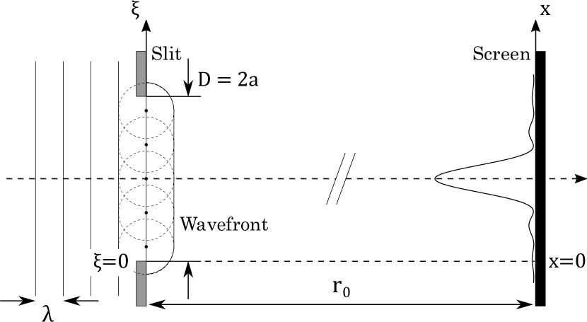
Figure 1: Diffraction of light from a single slit. Each solid line represents an undiffracted wavefront, while a solid curve represents a diffracted wavefront determined from Huygens’ wavelets at the aperture (dashed-line circles). Here, we define the wavelength $\lambda$, the aperture size $D=2a$, and the distance $r_{0}$ between the slit and the screen.

By comparing two functions $\tilde{h}$ [Eq. (12)] and $\tilde{h}_{E}$ [Eq. (18)], we can obtain exact relations that connect the two phenomena: to do so, we introduce dimensionless integration variables, $\hat{t}\equiv t^{\prime}/\Delta$ and $\hat{\xi}\equiv\xi/(2a)$. Then we have the phase function of the integrand for Eq. (12):

$$\Phi(\hat{t})=2\pi\nu^{(0)}\Delta(1-r)\hat{t}+2\pi\nu^{(1)}\Delta^{2}\frac{\hat{t}^{2}}{2}-\phi_{0}$$ (19)

and that for Eq. (18):

$$\Phi_{E}(\hat{\xi})=-4\pi N_{F}\frac{x}{a}\hat{\xi}+8\pi N_{F}\frac{\hat{\xi}^{2}}{2}+\pi N_{F}\left(\frac{x}{a}\right)^{2},$$ (20)

where $N_{F}$ is a so-called Fresnel number:

$$N_{F}=\frac{a^{2}}{\lambda r_{0}}.$$ (21)

Since Eqs. (19) and (20) are both functions of a dimensionless variable, one immediately obtains the following relations:

$$\nu^{(0)}\Delta(r-1) \Longleftrightarrow 2N_{F}\frac{x}{a},$$ (22)

$$\nu^{(1)}\Delta^{2} \Longleftrightarrow 4N_{F}.$$ (23)

In the theory of single-slit diffraction, a Fresnel number $N_{F}$ is often defined to characterize diffraction patterns with different configurations: for $N_{F}\ll 1$, where the screen is far from the slit, or where the slit aperture is narrow, a quadratic term in the phase $\Phi_{E}$ is negligible so that Fresnel’s formula is reduced to a Fourier transform of the shape of the aperture (i.e., Fraunhofer diffraction). On the other hand, for $N_{F}\gtrsim 1$, Fresnel’s formula is called a Fresnel transformation, and a resulting diffraction pattern is a perfect shadow of the aperture (i.e., Fresnel diffraction). By using the relation (23), a corresponding quantity is also defined in the FHO case as:

$$N_{F}^{(\text{FHO})}\equiv\frac{\nu^{(1)}\Delta^{2}}{4},$$ (24)

and the relation (22) is rewritten as

$$\frac{4N_{F}^{(\text{FHO})}}{\nu^{(1)}\Delta}\left(\nu_{f}-\nu^{(0)}\right)\Longleftrightarrow\frac{4N_{F}}{2a}x.$$ (25)

As is the case of the single-slit diffraction, systems with the same value of $N_{F}^{(\text{FHO})}$ will have a response function $\tilde{h}(r)$ of equivalent properties.

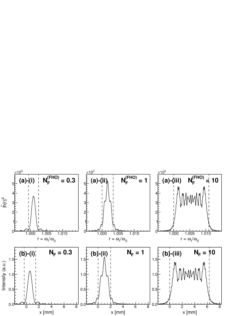
Figure 2: (a) Frequency responses $\tilde{h}(r)$ for (i) $N_{F}^{(\text{FHO})}=0.3$, (ii) $N_{F}^{(\text{FHO})}=1$ and (iii) $N_{F}^{(\text{FHO})}=10$, with $\nu^{(0)}=10~{}[\text{Hz}]$ and $\nu^{(1)}=0.0003~{}[\text{sec}^{-2}]$. The ranges of resonant frequencies evaluated by Eq. (26) are marked by dashed lines. (b) Diffraction patterns from a single slit for (i) $N_{F}=0.3$, (ii) $N_{F}=1$ and (iii) $N_{F}=10$ with $\lambda=1~{}[\mu\text{m}]$ and $r_{0}=1~{}[\text{m}]$. Dashed lines represent the positions of $x=\pm\delta\bar{x}$. For the definition of $\delta\bar{x}$, see the text.

Figures 2 (a) show the frequency responses $\tilde{h}(r)$ with different values of $N_{F}^{(\text{FHO})}$ (i.e., different values of $\Delta$). For reference, the intensity patterns of single-slit diffraction with the same values of $N_{F}$ (i.e., corresponding values of $a$) are plotted in Figs. 2 (b). For both the phenomena, a dramatic change of the frequency responses $\tilde{h}(r)$ (or the diffraction patterns) takes place around $N_{F}^{(\text{FHO})}\;(N_{F})\approx 1$. Furthermore, the behavior of $\tilde{h}(r)$ on $N_{F}^{(\text{FHO})}$ is in excellent agreement with that of the diffraction patterns on $N_{F}$.

The observed correspondence between the FHO and the single-slit diffraction can be interpreted as follows: it is obvious from Eq. (12) that the FHO with slowly-varying frequencies can be viewed as diffraction of waves in the frequency domain with time $t$ to be an independent variable, whereas the single-slit diffraction is discussed in the space domain. Thus, the frequency $\omega(t)$, moving in the frequency domain during a time window $\Delta$, is interpreted, in the case of single-slit diffraction, as the incremental space coordinate $\xi$ on the slit from $0$ to $2a$, and the constant frequency $\omega_{f}$ as an observation point, i.e., the space coordinate $x$ on the screen [see the relation (25)].

A key feature common to both phenomena is a quadratic term in the phase functions of Eqs. (19) and (20), which yields Fresnel integrals. In the FHO case, such a phase term comes from the difference of phase advance, i.e., the phase slippage between the oscillator and the driving force. In the single-slit diffraction case, on the other hand, such a phase term comes from Fresnel’s approximation of the optical path lengths of accumulated spherical waves. We summarize the correspondence relations between the FHO and the single-slit diffraction in Table 1.

Table 1: Correspondence relations between the FHO and the single-slit diffraction.

FHO	Single-slit Diffraction
$\omega_{f}$ (Driving force)	Position on screen
$\omega$ (Oscillator)	Position on slit
Variation of $\omega$ in $\Delta$, $2\pi\nu^{(1)}\Delta$	Aperture size $D=2a$
Phase slippage between oscillator and force	Variation of optical path length
A quantity $N_{F}^{(\text{FHO})}\equiv\nu^{(1)}\Delta^{2}/4$	Fresnel number $N_{F}=a^{2}/(\lambda r_{0})$

For quantitative discussion, we evaluate the range of resonant frequencies for the driving force, $2\delta\bar{\omega}_{f}$, using the analogies between the FHO and the single-slit diffraction. To clarify the situation, we start with the light diffraction case: for the Fraunhofer regime ($N_{F}\ll 1$), it is well known that the width $2\delta\bar{x}$ of a principal peak is obtained from the slit-screen distance $r_{0}$ and the angle $\theta$, which defines a destructive phase relation between the wavelets from the both edges of the aperture, and is given by $2\delta\bar{x}\approx 2r_{0}\theta\approx\lambda r_{0}/(2a)$. For the Fresnel regime ($N_{F}\gtrsim 1$), the width of a rectangular pattern is almost the same as that of the aperture, namely, $2\delta\bar{x}\approx 2a$. Now, the derivation of $\delta\bar{\omega}_{f}$ is straightforward: with the correspondence relations (24) and (25), we obtain:

$$2\delta\bar{\omega}_{f}=\begin{cases}2\pi/\Delta&\text{(for the Fraunhofer regime)}\\ 2\pi\nu^{(1)}\Delta&\text{(for the Fresnel regime)}.\end{cases}$$ (26)

The evaluated ranges for different values of $N_{F}^{(\text{FHO})}$ are indicated by dashed lines in Figs. 2 (a). As we see from the figures, our evaluation is valid both for the Fraunhofer and Fresnel regimes. We notice that, for the FHO case, the center of resonant frequencies is given by $\bar{\omega}_{f}=2\pi\nu^{(0)}+\pi\nu^{(1)}\Delta$.

As another example of the analogies between FHOs with time-varying frequencies and light diffraction, let us consider a HO with a time-varying natural frequency exposed continuously to a sinusoidal force with a constant frequency. Here, we suppose that the frequency $\omega(t)$ of the oscillator varies linearly and coincides with the frequency $\omega_{f}$ of the driving force at $t=0$. In this case, a particular solution is obtained just by setting $r=1$ and replacing $\Delta$ with $t$ in the response function of Eq. (12), namely:

$$\begin{split}\tilde{h}(t)\simeq&\frac{e^{-i\phi_{0}}}{\sqrt{2\nu^{(1)}}}\displaystyle\int^{\sqrt{2\nu^{(1)}}t}_{0}\exp\left(i\displaystyle\frac{\pi}{2}\tilde{t}^{2}\right)d\tilde{t}\\ =&\frac{e^{-i\phi_{0}}}{\sqrt{2\nu^{(1)}}}\left[C\left(\sqrt{2\nu^{(1)}}t\right)+iS\left(\sqrt{2\nu^{(1)}}t\right)\right],\end{split}$$ (27)

which is in turn a function of $t$, and thus describes the time evolution of the oscillation amplitude, together with the damping factor $A(t)$ [see Eq. (9)]. The expression of Eq. (27) is quite similar to a diffraction formula for so-called knife-edge diffraction. In what follows, we neglect the damping factor $A(t)$, which does not stem from the presence of the driving force, in order to highlight the response of the oscillator and to compare it to knife-edge diffraction.

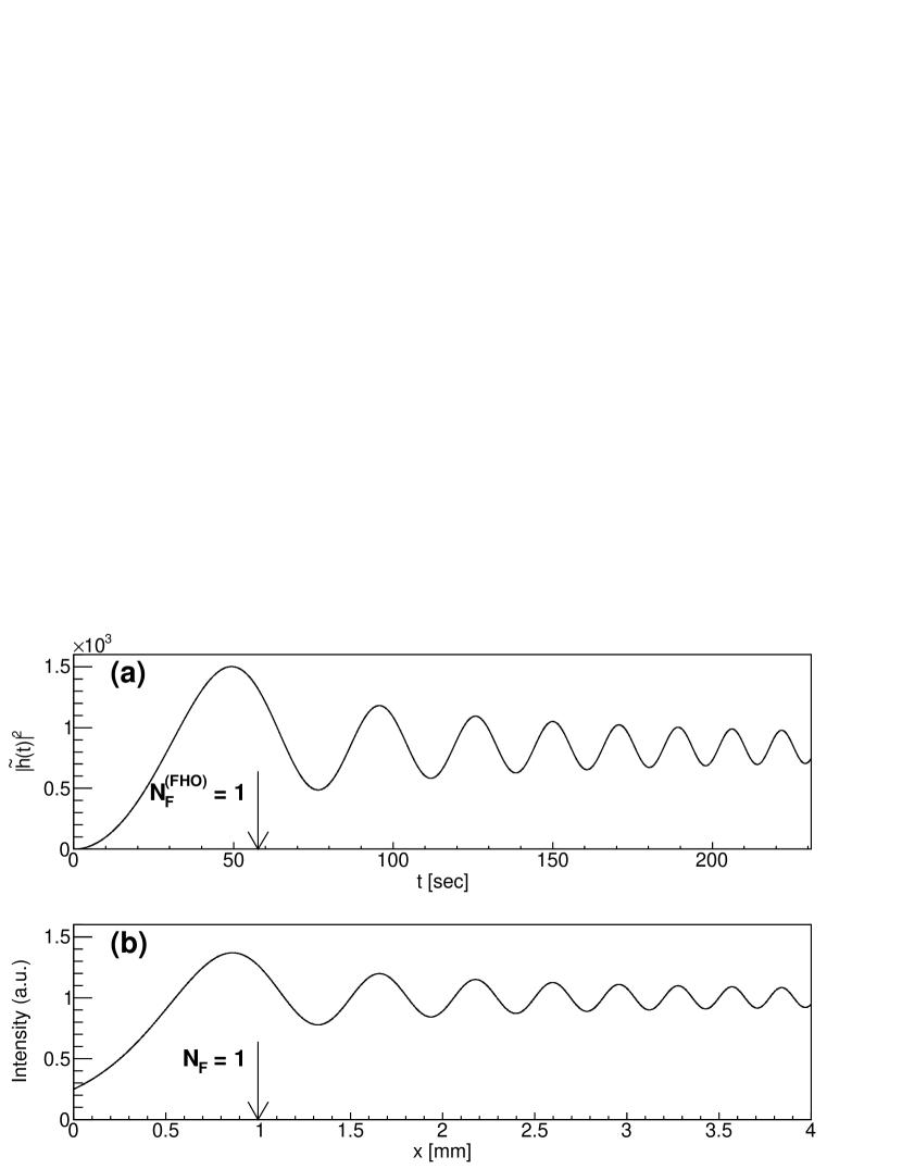
Figure 3: (a) Time evolution of the squared amplitude $|\tilde{h}(r)|^{2}$ with $\nu^{(0)}=10~{}[\text{Hz}]$ and $\nu^{(1)}=0.0003~{}[\text{sec}^{-2}]$. An arrow indicates the time $t=\delta t$ corresponding to $N_{F}^{(\text{FHO})}=1$. For the definition of $\delta t$, see the text. (b) Intensity pattern for light diffraction from a knife-edge obstacle with $\lambda=1~{}[\mu\text{m}]$ and $r_{0}=1~{}[\text{m}]$. The obstacle is placed at $x\leq 0$. An arrow indicates the screen position $x$ corresponding to $N_{F}=1$.

Taking the limit $2a\rightarrow+\infty$ in Eq. (18) gives the expression of $\tilde{h}_{E}$ for knife-edge diffraction:

$$\begin{split}\tilde{h}_{E}(x)=&\int^{+\infty}_{0}\exp\left[\frac{i\pi}{\lambda r_{0}}\left(\xi-x\right)^{2}\right]d\xi\\ =&\sqrt{\frac{\lambda r_{0}}{2}}\left[\left\{C\left(\sqrt{\frac{2}{\lambda r_{0}}}x\right)+\frac{1}{2}\right\}\right.\\ &+\left.i\left\{S\left(\sqrt{\frac{2}{\lambda r_{0}}}x\right)+\frac{1}{2}\right\}\right].\end{split}$$ (28)

Note that, by comparing the arguments of the Fresnel integrals in Eqs. (27) and (28), we can obtain a similar relation to Eq. (23), namely:

$$\nu^{(1)}t_{\text{obs}}^{2}\Longleftrightarrow\frac{x_{\text{obs}}^{2}}{\lambda r_{0}},$$ (29)

where $t_{\text{obs}}$ and $x_{\text{obs}}$ are the observation time and position for the FHO and knife-edge diffraction cases, respectively.

Figure 3 (a) illustrates the time evolution of the squared oscillation amplitude (or, equivalently, the energy of the oscillator), together with an intensity pattern for light diffraction from a knife-edge obstacle [Fig. 3 (b)]. We see that the time evolution of the oscillation energy behaves like a knife-edge diffraction pattern: that is, the energy increases monotonically until $t\lesssim 60~{}[\text{sec}]$ and then exhibits small beating (in other word, we could say that the oscillator is in a quasi-stationary state). Asymptotically, it approaches to [see Eq. (27)]:

$$|\tilde{h}(t)|^{2}\xrightarrow{t\rightarrow+\infty}\displaystyle\frac{1}{2\nu^{(1)}}\left[C^{2}(+\infty)+S^{2}(+\infty)\right]=\displaystyle\frac{1}{4\nu^{(1)}}.$$ (30)

The time duration $\delta t$ in which the driving force efficiently supplies kinetic energy to the oscillator is estimated by using the analogies: in knife-edge diffraction, a ”good measure” of the fringe width of diffraction patterns, $\delta x$, is given by the condition that the corresponding Fresnel number, $N_{F}=\delta x^{2}/(\lambda r_{0})$, becomes unity [see Fig. 3 (b)]. Similarly, from Eq. (29), we have the time duration $\delta t$:

$$\delta t=\frac{1}{\sqrt{\nu^{(1)}}}\approx 60~{}[\text{sec}],$$ (31)

with $\nu^{(1)}=0.0003~{}[\text{sec}^{-2}]$.

IV Summary

In summary, we investigated a simple FHO with slowly-varying frequencies. We demonstrated that the time evolution of such a system can be written in a simplified form using Fresnel integrals. As a result, we found that FHOs with slowly-varying frequencies can be viewed as diffraction of waves in the frequency domain, and therefore are equivalent to diffraction of light. Also we showed two examples to see the similarities between the two phenomena, and derived simple formulae for the quantities which characterize the systems. We expect that our formulation as well as such simple formulae is applied to, e.g., accelerator physics and provides a simple and intuitive approach to the phenomenon of ”resonance crossing”, which is a central issue in a ring-type particle accelerator design [16, 17]. As a matter of fact, we applied our formulation to the design of an aborted-beam-handling system for a new synchrotron light source accelerator [18]. In this system, a sinusoidal force is applied to aborted beams, whose betatron frequency varies with time due to energy loss by synchrotron radiation. A proper choice of frequency of the sinusoidal force is essential to enlarge the amplitude of betatron oscillation and to reduce the beam density. Our findings will be also applicable to plasma physics, where the problem of passage through resonance with slowly-varying parameters is of great importance [19].

Appendix A Derivation of Green’s function

In this appendix, we present the derivation of the Green’s function of Eq. (7). With the aid of the method of ”variation of constants”, the Green’s function of an inhomogeneous differential equation such as Eq. (2) is in general written in the form:

$$\begin{split}G(t,t^{\prime})&=\frac{\left|\begin{array}[]{cc}x_{1}(t^{\prime})&x_{2}(t^{\prime})\\ x_{1}(t)&x_{2}(t)\end{array}\right|}{W(x_{1},x_{2})(t^{\prime})}\\ &\equiv\frac{x_{1}(t^{\prime})x_{2}(t)-x_{1}(t)x_{2}(t^{\prime})}{x_{1}(t^{\prime})\dot{x}_{2}(t^{\prime})-\dot{x}_{1}(t^{\prime})x_{2}(t^{\prime})},\end{split}$$ (32)

where $x_{1}$ and $x_{2}$ are independent solutions for the corresponding homogeneous differential equation, and $W$ is the Wronskian. Thus, in our case, the problem comes down to solving the following homogeneous equation:

$$\ddot{x}+\omega^{2}(t)x=0.$$ (33)

To solve the above equation, we use the so-called eikonal approximation [20]; that is, it is assumed that a solution of Eq. (33) is of the form:

$$x(t)=a(t)e^{i\varphi(t)},$$ (34)

where the envelope function $a(t)$ varies very slowly compared to oscillation of $x(t)$, namely:

$$\frac{\ddot{a}(t)}{a(t)}\ll\omega^{2}(t).$$ (35)

Substituting Eq. (34) in Eq. (33) and using the condition (35), we obtain:

$$\left[\dot{\varphi}(t)\right]^{2}= \omega(t)^{2},$$ (36)

$$2\dot{a}(t)\dot{\varphi}(t)+a(t)\ddot{\varphi}(t)= 0.$$ (37)

It follows from Eq. (36) that:

$$\varphi(t)=\pm\left[\int^{t}_{0}\omega(\tau)d\tau+\varphi_{0}\right],$$ (38)

where $\varphi_{0}$ is an integration constant.

The substitution of Eq. (38) into Eq. (37) gives:

$$\frac{d}{dt}\left[\ln a(t)+\frac{1}{2}\ln\omega(t)\right]=0,$$ (39)

and we have:

$$a(t)=\frac{\alpha}{\sqrt{\omega(t)}},$$ (40)

where $\alpha$ is a constant.

Thus, two independent solution of Eq.(34) are given by:

$$x_{1,2}(t)=\frac{\alpha}{\sqrt{\omega(t)}}\exp\left[\pm i\left(\int^{t}_{0}\omega(\tau)d\tau+\varphi_{0}\right)\right],$$ (41)

and the substitution of Eq. (41) into Eq. (32) yields the Green’s function of Eq. (7). Note that the condition (35) is clearly fulfilled under the assumption (1).

References

• Feynman et al. [1971] R. P. Feynman, R. B. Leighton, and M. Sands, The Feynman Lectures on Physics, 1st ed., Vol. 1 (Addison Wesley, 1971).
• Goldstein et al. [2001] H. Goldstein, C. P. Poole Jr., and J. L. Safko, Classical Mechanics, 3rd ed. (Addison Wesley, 2001).
• Buchanan [2019] M. Buchanan, Nature Physics 15, 203 (2019).
• Bleck-Neuhaus [2018] J. Bleck-Neuhaus, arXiv:1811.08353 [phisics.hist-ph] (2018).
• Zwillinger [2014] D. Zwillinger, Tables of Integrals, Series, and Products, 8th ed. (Academic Press, 2014).
• Sommerfeld [2004] A. Sommerfeld, Mathematical Theory of Diffraction (Birkhaeuser, 2004).
• Hecht [2016] E. Hecht, Optics, 5th ed. (Pearson, 2016).
• Jenkins and White [2001] F. A. Jenkins and H. E. White, Fundamentals of Optics, 4th ed. (McGraw-Hill Science Engineering, 2001).
• Born and Wolf [2019] M. Born and E. Wolf, Principles of Optics, 7th ed. (Cambridge University Press, 2019).
• Note [1] The same discussion can be made even when a damping term is included, as long as its effect is sufficiently weak.
• Note [2] Here, we are interested in a particular solution because it contains all the effects of the driving force.
• Landau and Lifshitz [1982] L. D. Landau and E. M. Lifshitz, Mechanics, 3rd ed. (Butterworth-Heinemann, 1982) Chap. 7, Sect. 49.
• Park et al. [2011] Y. Park, Y. Do, and J. M. Lopez, Phys. Rev. E 84, 056604 (2011).
• Bourquard and Noiray [2019] C. Bourquard and N. Noiray, Phys. Rev. E 100, 047001 (2019).
• Pippard [2009] A. Pippard, Responce and Stability: An Introduction to the Physical Theory (Cambridge University Press, 2009).
• Chao and Month [1974] A. W. Chao and M. Month, Nucl. Instrum. Methods 121, 129 (1974).
• Franchetti and Zimmermann [2012] G. Franchetti and F. Zimmermann, Phys. Rev. Lett. 109, 234102 (2012).
• [18] T. Hiraiwa et al., Manuscript in preparation.
• Armon and Friedland [2016] T. Armon and L. Friedland, J. Plasma Phys. 82, 705820501 (2016).
• Sommerfeld [1964] A. Sommerfeld, Lecture on Theoretical Physics: Optics (Academic Press, 1964).