Biomechanical surrogate modelling using stabilized vectorial greedy kernel methods

Abstract

Greedy kernel approximation algorithms are successful techniques for sparse and accurate data-based modelling and function approximation. Based on a recent idea of stabilization [11] of such algorithms in the scalar output case, we here consider the vectorial extension built on VKOGA [12]. We introduce the so called $\gamma$-restricted VKOGA, comment on analytical properties and present numerical evaluation on data from a clinically relevant application, the modelling of the human spine. The experiments show that the new stabilized algorithms result in improved accuracy and stability over the non-stabilized algorithms.

1 Introduction

Kernel methods are used in various fields of machine learning or pattern analysis. They yield efficient and flexible ways to recover functions from data since they can deal with arbitrarily scattered points. The combination of their flexibility with the strong mathematical theory about e.g. existence, convergence, stability make them a nice tool for applications [3, 10].
In this paper we apply a recently introduced idea that has lead to a new class of stabilized greedy kernel algorithms [11], extend it to vectorial function approximation and apply it to a real life setting from research in biomechanics. Some theoretic statements can be extended from the scalar to the vectorial case. All in all these stabilized methods provide further flexibility and are able to efficiently mitigate the problem of having numerical instabilities.
The paper is organized as follows. To begin with we recall in Section 2 some basics about kernel interpolation with a focus on greedy kernel approximation and explain the stabilized extension. Section 3 gives background information about our application settings and the use of kernel methods. The following Section 4 explains the conducted numerical experiments as well as the practical results. Section 5 concludes with a summary and an outlook.

2 Stabilized VKOGA algorithm

We start with a nonempty set $\Omega\subset\mathbb{R}^{d}$. A real-valued kernel is a symmetric function $k:\Omega\times\Omega\rightarrow\mathbb{R}$. For arbitrary points $X_{N}:=\{x_{1},..,x_{N}\}\subset\Omega$ the kernel matrix $A\in\mathbb{R}^{N\times N}$ is a symmetric matrix with entries $A_{ij}=k(x_{i},x_{j})$. If this kernel matrix is positive semi-definite for any set of points $X_{N}\subset\Omega$, then the kernel is called positive definite. If the kernel matrix is even positive definite for any set of pairwise distinct points, then the kernel is called strictly positive definite. In the following we will focus on this case of strictly positive definite kernels and we refer to the monographs [3, 10] for more details.
For any such kernel there is a unique Hilbert space of functions, namely the native space $(\mathcal{H}_{k}(\Omega),(\cdot,\cdot)_{\mathcal{H}_{k}(\Omega)})$, which is a Reproducing Kernel Hilbert Space (RKHS). A popular choice is given by radial basis function kernels, i.e. the kernel can be expressed with the help of some function $\Phi$ and a kernel parameter $\epsilon\in\mathbb{R}$ as $k(x,y)=\Phi(\epsilon\|x-y\|)$. Examples are given by the Gaussian kernel $\Phi_{\text{Gauss}}(r)=\exp(-(\epsilon\cdot r)^{2})$and the linear Matérn kernel $\Phi(r)=(1+r)\cdot\exp(-r)$. The decay of the Fourier transform of those radial basis functions is decisive for their properties. The Fourier transform of the Gaussian decays exponentially, whereas the Fourier transform of the linear Matérn decays only algebraically.

In such RKHS the interpolation of functions - or more general data based approximation tasks - can be analyzed. For a given function $f\in\mathcal{H}_{k}(\Omega)$ and some interpolation points $X_{N}$ the interpolant $s_{N}$ is given by the orthogonal projection $\Pi_{V(X_{N})}(f)$ of $f$ onto $V(X_{N}):=\{k(\cdot,x_{i}),x_{i}\in X_{N}\}$ and thus can be expressed as

$$s_{N}(\cdot)=\Pi_{V(X_{N})}(f)=\sum_{i=1}^{N}\alpha_{i}k(\cdot,x_{i}),\;\;\alpha_{i}\in\mathbb{R},1\leq i\leq N.$$

In some applications the data is affected by noise, so it does not make sense to interpolate the given values, while it is rather advisable to approximate them while taking some regularization into account. For this one can consider minimizing $\sum_{i=1}^{N}\|f(x_{i})-s_{N}(x_{i})\|_{2}^{2}+\lambda\cdot\|s_{N}\|_{\mathcal{H}_{k}(\Omega)}^{2}$ which corresponds to solving the linear system

$$(A+\lambda\cdot I)\alpha=y$$ (1)

with $y=(f(x_{i}))_{i=1}^{N}$. To measure the interpolation error $\|f-\Pi_{V(X_{N})}(f)\|_{L^{\infty}}$ one can introduce the Power function $P_{X_{N}}:\Omega\rightarrow\mathbb{R}$ as

$$P_{N}(x):=P_{X_{N}}(x)=\sup_{0\neq f\in\mathcal{H}_{k}(\Omega)}\frac{|f(x)-\Pi_{V(X_{N})}(f)(x)|}{\|f\|_{\mathcal{H}_{k}(\Omega)}}.$$ (2)

From this definition we can directly conclude

$$|f(x)-\Pi_{V(X_{N})}(f)(x)|\leq P_{N}(x)\cdot\|f\|_{\mathcal{H}_{k}(\Omega)}.$$

For the analysis of the kernel interpolants geometric quantities about the distribution of the interpolation points are important. The fill distance $h_{N}$ and the separation distance $q_{N}$ are defined as

$$h_{N}:=\sup_{x\in\Omega}\min_{x_{i}\in X_{N}}\|x-x_{i}\|_{2},\hskip 28.45274ptq_{N}:=\min_{x_{i}\neq x_{j}\in X_{N}}\|x_{i}-x_{j}\|_{2}.$$ (3)

A priori it is unclear how to select good interpolation points for a given set of data or some functions. To circumvent this, one applies greedy methods which start with an empty set $X_{0}=\{\}$ and iteratively add another interpolation point according to some selection criterion, $X_{N+1}=X_{N}\cup\{x_{N+1}\}$.
There are three main selection criteria in the literature, namely $f$-greedy, $f/P$-greedy and $P$-greedy [9, 1, 6] which choose the next point from $\Omega$ according to some indicator. For the vectorial case, for $x\in\Omega$ they are:

1. $f$-greedy:         $\eta_{f}^{(N)}(x)=\|f(x)-\Pi_{V(X_{N})}(f)(x)\|_{2}$

2. $P$-greedy:        $\eta_{P}^{(N)}(x)=P_{X_{N}}(x)$

3. $f/P$-greedy:     $\eta_{f/P}^{(N)}(x)=\|f(x)-\Pi_{V(X_{N})}(f)(x)\|_{2}/P_{X_{N}}(x)$.

In order to create a scale of selection criteria which lie in between those known criteria, one introduces a restriction parameter $\gamma\in(0,1]$ and a restricted set $\Omega_{\gamma}^{(N)}:=\{x\in\Omega,P_{N}(x)\geq\gamma\cdot\|P_{N}\|_{\infty}\}$ and chooses the next interpolation point within $\Omega_{\gamma}^{(N)}$ according to some standard selection criterion. This works since the Power function is scalar valued and the interpolation points are shared among all dimensions. For $\gamma=1$ it holds $\Omega_{\gamma}^{(N)}=\{x\in\Omega,P_{N}(x)=\|P_{N}\|_{\infty}\}$, thus we obtain the standard $P$-greedy algorithm for any selection criterion $\eta^{(N)}(x)$. For $\gamma=0$ it holds $\Omega_{\gamma}^{(N)}=\Omega$, thus we obtain the unrestricted algorithm. The naming restricted is obviously related to the restriction of the set $\Omega$ to $\Omega_{\gamma}^{(N)}$, the name stabilized is motivated by part of the results within [11], which are summarized in Theorem 1. If the maximum within a selection rule is not unique, any point realizing the maximum can be picked.

As an example, the $\gamma$-stabilized $f$-greedy chooses the next point according to

$$x_{N+1}=\operatorname*{arg\max}_{x\in\Omega_{\gamma}^{(N)}}\|f(x)-\Pi_{V(X_{N})}(f)(x)\|_{2}.$$

Several rigorous analytical statements can be derived for this kind of algorithms and we will summarize a few of them in the following Theorem 1. The proofs are straightforward consequences of those which can be found in [11].

Theorem 1

Assume that $\Omega\subset\mathbb{R}^{d}$ is a compact domain which satisfies an interior cone condition and has a Lipschitz boundary. Suppose that $k$ is a translational invariant kernel such that its native space is norm equivalent to the Sobolev space $H^{\tau}(\Omega)$ with $\tau>d/2$. Then any $\gamma$-stabilized algorithm applied to a function in $f\in\mathcal{H}_{k}(\Omega)$ gives a sequence of point sets $X_{N}\subset\Omega$ such that it holds:

• Lower and upper bound on the Power function:

  $$c_{P}\cdot N^{\frac{1}{2}-\frac{\tau}{d}}\leq\|P_{N}\|_{L^{\infty}(\Omega)}\leq C_{P}\cdot\gamma^{-2}\cdot N^{\frac{1}{2}-\frac{\tau}{d}}.$$

• Asymptotic uniform point distribution:

  $$\rho_{X_{N}}:=\frac{h_{N}}{q_{N}}\leq c\cdot\gamma^{-4}~{}~{}\forall N\in\mathbb{N}.$$

• Lower and upper bounds on the smallest eigenvalue:

  $$c_{1}\cdot\gamma^{8\tau-4d-4}\cdot N^{1-2\tau/d}\leq\lambda_{\min}(X_{N})\leq c_{2}\cdot\gamma^{-4}\cdot N^{1-2\tau/d}.$$

Finally we want to point out that the $\gamma$–parameter only affects the choice of points, i.e. it modifies the greedy selection. However, if given points are used the $\gamma$ parameter does not change the computed interpolant anymore. This is in contrast to the parameters $\lambda$ and $\epsilon$, which modify also the interpolant if points are given.

From Theorem 1 we can conclude that the product $\lambda_{\min}\cdot\|P_{N}\|_{\infty}^{2}$ is bounded from both sides for $\gamma>0$. This motivates to take the value of the Power function of the previously chosen point as a measure of stability. This will be used in Equation (4) to implement a stopping criterion based on stability.

3 Application to spine modelling

Biomechanical models of the human spine account for the most significant structures which carry the load of daily life. That are mostly the ligaments, the muscles with both passive and active contributions and the intervertebral discs (IVDs), of course. An IVD, in this sense, can be seen as a combination of both the defining structure for the degrees of freedom between two vertebral bodies and the force and rotational moment transducing elements between these two bones, cf. Figure 1.

Mostly, IVDs are modelled by a linear approximation of forces and rotational moments calculated according to the respective displacements, e.g. [5]. Alternatively, as long as quasi-static movements are studied, very detailed, finite element models of isolated IVDs or a combination of few spinal segments are used [2]. Another approach to model a reduced IVD used a polynomial approximation and showed that the classical linear approximations overestimate actual stiffnesses in the working range [4, 7]. This observation gave rise to the idea of looking into an even more sophisticated mapping of displacements on the input to output forces and rotational moments.input-output mapping in three spacial dimensions.

Obviously, kernel modelling seems to be an ideal approach for this need. First, kernel surrogates promise to capture the mapping characteristics well, second, extensions to higher input and output dimensions seem feasible and third, compared to respective detailed finite element models surrogate models evaluate the mapping stunningly fast [13].

Assuming symmetry in the sagittal and frontal plane, an input-output relation $f:\mathbb{R}^{3}\rightarrow\mathbb{R}^{3}$ is considered and studied, here.

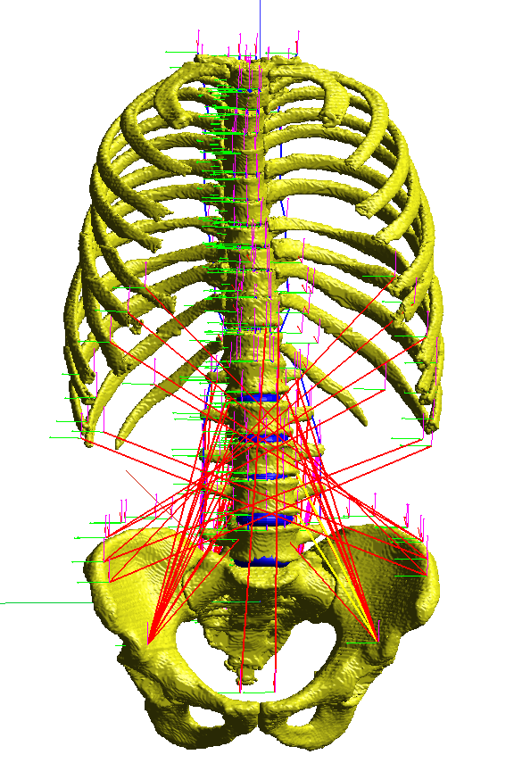
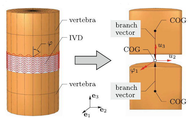
Figure 1: Visualization of the biomechanical model. On the left the whole spine model is depicted, on the right the modelling scheme of an IVD reduced to a 3-d force/torque element is shown [4].

4 Numerical experiments

The considered dataset consists of 1370 input points in $\mathbb{R}^{3}$ with corresponding output points in $\mathbb{R}^{3}$. 1238 points are used for training and validation, the remaining points are used as a test set. No scaling is applied to the data. In order to show the flexibility and thus improved accuracy of the stabilized algorithms on the presented data set, we compute unstabilized approximants, used as base models, as well as stabilized models for the $f$- and the $f/P$-greedy algorithm. For both the unstabilized and stabilized models we also use regularization in a second step. The experiments are related to those in [8, 13], however due to different setups they are not identical.
The base models are given by standard kernel surrogates where the point selection is done either with vectorial $f$-greedy or $f/P$-greedy. To evaluate good parameters, first of all a $5$-fold cross validation is run on $20$ logarithmic equally spaced kernel parameters $\epsilon$. The best $\epsilon$ value is used for a second step, where the best $\lambda$ parameter from Equation (1) is evaluated with help of another $5$-fold cross validation. For this we use $20$ logarithmic equally spaced values between $10^{-16}$ and $10^{3}$. As an error measure we use the Root Mean Square Error (RMSE)

$$E_{\text{RMSE}}(s,X,Y)=\left(\frac{1}{|X|}\cdot\sum_{i=1}^{|X|}\|s(x_{i})-y_{i}\|_{2}^{2}\right)^{1/2}.$$

The stabilized models are given by kernel surrogates where the points are selected with help of stabilized vectorial $f$- or $f/P$-greedy algorithms. We start by using the same kernel parameter $\epsilon$ which was selected for the base model and run instead a $5$-fold cross validation on $11$ equally spaced stabilization parameters $\gamma\in[0,1]$. As a second step we evaluate again the best $\lambda$ parameter with help of a $5$-fold cross validation. This procedure keeps the computation time similar to the base model.

The used hyperparameters are summarized in Table 1. For the experiments the linear Matérn kernel is used since it satisfies all the prerequisites of Theorem 1.

$k$	$\epsilon_{\min}$	$\epsilon_{\max}$	$n_{\epsilon}$	$\gamma_{\min}$	$\gamma_{\max}$	$n_{\gamma}$	$\lambda_{\min}$	$\lambda_{\max}$	$n_{\lambda}$
5	$10^{-2}$	$10^{1}$	$20$	$0$	$1$	$11$	$10^{-16}$	$10^{3}$	20

Table 1: Overview of the hyperparameter ranges. The $\gamma$ values are equally spaced, the others are logarithmically equally spaced.

The greedy selection algorithms stop either when all points within the training set are selected or if some threshold on the residual or on the Power function is met. As a tolerance on the residual we use $\tau_{f}=10^{-7}$, that means the selection is stopped if $\max\|s_{N}(x_{i})-y_{i}\|_{2}<\tau_{f}$ is met. As a tolerance for the Power function we use $\tau_{P}=10^{-3}$ and the selection is stopped if

$$P_{N}(x_{N+1})<\tau_{P}.$$ (4)

We remark that this last criterion is directly linked to the stability. If points with small Power function value are selected, it means that the interpolation points cluster. We recall that this means in particular that $\lambda_{\min}(X_{N})$ is below a certain threshold, making further computations unstable. Moreover, although a thorough discussion on the fine tuning of these thresholds is beyond the scope of this paper, we remark that the chosen values appear to be reasonable in this setting since they are sufficient to achieve the desired accuracy, while avoiding instabilities.

Table 2 lists both the hyperparameters which were selected by the cross-validations and the resulting accuracies of the interpolants. The $E_{\max,\text{rel}}$ and the $E_{\text{RMSE},\text{rel}}$ errors are defined according to

$$E_{\max,\text{rel}} :=\max_{i=1,..,|X|}\|s(x_{i})-y_{i}\|_{2}/\|y_{i}\|_{2},$$

$$E_{\text{RMSE},\text{rel}} :=\left(\frac{1}{|X|}\cdot\sum_{i=1}^{|X|}\frac{\|s(x_{i})-y_{i}\|_{2}^{2}}{\|y_{i}\|_{2}^{2}}\right)^{1/2}.$$

	$f$-greedy			$f/P$-greedy
	Hyperparameters	Results		Hyperparameters	Results
base	$\epsilon_{\text{base}}\hskip 1.13809pt=6.158\cdot 10^{-2}$	$E_{\max}\hskip 14.51091pt=347.22$		$\epsilon_{\text{base}}\hskip 1.13809pt=4.281\cdot 10^{-2}$	$E_{\max}\hskip 14.51091pt=4729.19$
	$\gamma_{\text{base}}\hskip 0.56905pt=0$	$E_{\text{RMSE}}\hskip 8.53581pt=39.58$		$\gamma_{\text{base}}\hskip 0.56905pt=0$	$E_{\text{RMSE}}\hskip 8.53581pt=1104.12$
	$\lambda_{\text{base}}=10^{-5}$	$E_{\max,\text{rel}}\hskip 6.25958pt=6.95$		$\lambda_{\text{base}}=10^{-2}$	$E_{\max,\text{rel}}\hskip 6.25958pt=116.02$
	$n_{\text{base}}=142$	$E_{\text{RMSE},\text{rel}}=9.00\cdot 10^{-1}$		$n_{\text{base}}=63$	$E_{\text{RMSE},\text{rel}}=14.83$
stabilized	$\epsilon_{\text{stab}}\hskip 1.13809pt=\epsilon_{\text{base}}$	$E_{\max}\hskip 14.51091pt=344.91$		$\epsilon_{\text{stab}}\hskip 1.13809pt=\epsilon_{\text{base}}$	$E_{\max}\hskip 14.51091pt=234.40$
	$\gamma_{\text{stab}}\hskip 0.56905pt=0.5$	$E_{\text{RMSE}}\hskip 8.53581pt=35.69$		$\gamma_{\text{stab}}\hskip 0.56905pt=0.2$	$E_{\text{RMSE}}\hskip 8.53581pt=30.22$
	$\lambda_{\text{stab}}=10^{-5}$	$E_{\max,\text{rel}}\hskip 6.25958pt=1.79\cdot 10^{-1}$		$\lambda_{\text{stab}}=10^{-15}$	$E_{\max,\text{rel}}\hskip 6.25958pt=6.77\cdot 10^{-1}$
	$n_{\text{stab}}=690$	$E_{\text{RMSE},\text{rel}}=2.26\cdot 10^{-2}$		$n_{\text{stab}}=358$	$E_{\text{RMSE},\text{rel}}=7.97\cdot 10^{-2}$

Table 2: Overview of the selected hyperparameter and the accuracies of the kernel models.

In the left plot of Figure 4 the number of selected points during the cross validation are depicted for the $f/P$-greedy. One can see ‘ that increasing the stabilization parameter $\gamma$ yields more interpolation points. The reason is that the stopping criterion $P_{N}(x_{N+1})<\tau_{P}$ is reached later since the selected points are distributed more uniformly as quantified in Theorem 1 and thus the greedy algorithms run further. We omit plotting results for the $f$-greedy as they do not differ considerably. Eventually these further interpolation points yield a better interpolation accuracy, which can be seen in Table 2. Especially the maximal relative error $E_{\max,\text{rel}}$ and the relative RMSE error $E_{\text{RMSE, rel}}$ are improved. In the right plot of Figure 4 the error decay for $f/P$-greedy depending on the number of chosen points during the selection (first step of training) is visualized for the $E_{\text{RMSE}}$ error. One can observe that the algorithm stops quite early since the stability stopping criterion (4) is met. Larger stabilization parameters yield a slower drop, however more interpolation points.

&

Figure 2: Left plot: Number of chosen interpolation points (y-axis) during the 5-fold cross validation procedure for $f/P$-greedy in dependence of the restriction parameter $\gamma\in\{0,0.1,..,1\}$ (x-axis). The black crosses indicate the five numbers of chosen points during the validation, the red line describes the mean value of those. Right plot: $E_{\text{RMSE}}$ error decay (y-axis) during the training of the $f/P$-greedy model depending on the number of interpolation points (x-axis) for the unstabilized model ($\gamma=0$), the stabilized model with validated $\gamma$-parameter ($\gamma=0.2$) and the fully stabilized model ($\gamma=1$, i.e. $P$-greedy).

5 Conclusion and Outlook

In this paper a vectorial extension of a recent idea of stabilization of greedy kernel approximation algorithms was introduced and analytical properties were stated. A numerical application was addressed using data that emerge in the simulation of the human spine and the stabilization led to significant improvements in terms of accuracy and stability due to a better point distribution. A two-step approach was used to combine the stabilization with regularization. In future work we will consider a combined approach of stabilization and regularization and use data with more input and output dimensions. Ultimatively we aim at using real patient data and dataset extension approaches by using invariances and symmetries or the use of invariant kernels.

Acknowledgements: The authors acknowledge the funding of the project by the Deutsche Forschungsgemeinschaft (DFG, German Research Foundation) under Germany’s Excellence Strategy - EXC 2075 - 390740016.

References

- [1] S. De Marchi, R. Schaback, and H. Wendland. Near-optimal data-independent point locations for radial basis function interpolation. Adv. Comput. Math., 23(3):317–330, 2005.
- [2] M. Dreischarf, T. Zander, A. Shirazi-Adl, C. Puttlitz, C. Adam, C. Chen, V. Goel, A. Kiapour, Y. Kim, K. Labus, J. Little, W. Park, Y. Wang, H. Wilke, A. Rohlmann, and H. Schmidt. Comparison of eight published static finite element models of the intact lumbar spine: Predictive power of models improves when combined together. Journal of Biomechanics, 47(8):1757 – 1766, 2014.
- [3] G. E. Fasshauer and M. McCourt. Kernel-Based Approximation Methods Using MATLAB, volume 19 of Interdisciplinary Mathematical Sciences. World Scientific Publishing Co. Pte. Ltd., Hackensack, NJ, 2015.
- [4] N. Karajan, O. Röhrle, W. Ehlers, and S. Schmitt. Linking continuous and discrete intervertebral disc models through homogenisation. Biomechanics and Modeling in Mechanobiology, 12(3):453–66, Jun 2013.
- [5] N. M. B. Monteiro, M. P. T. da Silva, J. O. M. G. Folgado, and J. P. L. Melancia. Structural analysis of the intervertebral discs adjacent to an interbody fusion using multibody dynamics and finite element cosimulation. Multibody System Dynamics, 25(2):245–270, Feb 2011.
- [6] S. Müller. Komplexität und Stabilität von kernbasierten Rekonstruktionsmethoden (Complexity and Stability of Kernel-based Reconstructions). PhD thesis, Fakultät für Mathematik und Informatik, Georg-August-Universität Göttingen, 2009.
- [7] T. Rupp, W. Ehlers, N. Karajan, M. Günther, and S. Schmitt. A forward dynamics simulation of human lumbar spine flexion predicting the load sharing of intervertebral discs, ligaments, and muscles. Biomechanics and Modeling in Mechanobiology, 14(5):1081–1105, 2015.
- [8] G. Santin and B. Haasdonk. Kernel methods for surrogate modelling. Technical Report arXiv:1907.10556, University of Stuttgart, 2019. to appear in the MOR Handbook, de Gruyter.
- [9] R. Schaback and H. Wendland. Adaptive greedy techniques for approximate solution of large RBF systems. Numer. Algorithms, 24(3):239–254, 2000.
- [10] H. Wendland. Scattered Data Approximation, volume 17 of Cambridge Monographs on Applied and Computational Mathematics. Cambridge University Press, Cambridge, 2005.
- [11] T. Wenzel, G. Santin, and B. Haasdonk. A novel class of stabilized greedy kernel approximation algorithms: Convergence, stability & uniform point distribution. arXiv e-prints, page arXiv:1911.04352, Nov 2019.
- [12] D. Wirtz and B. Haasdonk. A vectorial kernel orthogonal greedy algorithm. Dolomites Res. Notes Approx., 6:83–100, 2013.
- [13] D. Wirtz, N. Karajan, and B. Haasdonk. Surrogate modeling of multiscale models using kernel methods. International Journal for Numerical Methods in Engineering, 101, 01 2015.
- [14] D. Wittwar, G. Santin, and B. Haasdonk. Interpolation with uncoupled separable matrix-valued kernels. Dolomites Res. Notes Approx., 11:23–29, 2018.