The RAdial Velocity Experiment (RAVE):
Parameterisation of RAVE spectra based on
convolutional neural networks

Abstract

Context. Data-driven methods play an increasingly important role in the field of astrophysics. In the context of large spectroscopic surveys of stars, data-driven methods are key in deducing physical parameters for millions of spectra in a short time. Convolutional neural networks (CNNs) enable us to connect observables (e.g. spectra, stellar magnitudes) to physical properties (atmospheric parameters, chemical abundances, or labels in general).

Aims. We test whether it is possible to transfer the labels derived from a high-resolution stellar survey to intermediate-resolution spectra of another survey by using a CNN.

Methods. We trained a CNN, adopting stellar atmospheric parameters and chemical abundances from APOGEE DR16 (resolution $R=22500$) data as training set labels. As input, we used parts of the intermediate-resolution RAVE DR6 spectra ($R\sim 7\,500$) overlapping with the APOGEE DR16 data as well as broad-band ALL_WISE and 2MASS photometry, together with Gaia DR2 photometry and parallaxes.

Results. We derived precise atmospheric parameters $\textit{T}_{\text{eff}}$, $\text{log}(\textit{g})$, and $[\text{M}/\text{H}],$ along with the chemical abundances of $[\text{Fe}/\text{H}]$, $[\alpha/\text{M}]$, $[\text{Mg}/\text{Fe}]$, $[\text{Si}/\text{Fe}]$, $[\text{Al}/\text{Fe}]$, and $[\text{Ni}/\text{Fe}]$ for $420\,165$ RAVE spectra. The precision typically amounts to 60 K in $\textit{T}_{\text{eff}}$, 0.06 in $\text{log}(\textit{g})$ and 0.02-0.04 dex for individual chemical abundances. Incorporating photometry and astrometry as additional constraints substantially improves the results in terms of the accuracy and precision of the derived labels, as long as we operate in those parts of the parameter space that are well-covered by the training sample. Scientific validation confirms the robustness of the CNN results. We provide a catalogue of CNN-trained atmospheric parameters and abundances along with their uncertainties for $420\,165$ stars in the RAVE survey.

Conclusions. CNN-based methods provide a powerful way to combine spectroscopic, photometric, and astrometric data without the need to apply any priors in the form of stellar evolutionary models. The developed procedure can extend the scientific output of RAVE spectra beyond DR6 to ongoing and planned surveys such as Gaia RVS, 4MOST, and WEAVE. We call on the community to place a particular collective emphasis and on efforts to create unbiased training samples for such future spectroscopic surveys.

1 Introduction

Stellar chemical abundances are key tracers of the star formation history of the Milky Way and they are indicators of the timing of successive star formation events. The relative chemical abundances of stars thus allow us to disentangle stellar populations and to put constraints on the nucleosynthetic origin of the respective elements Yoshii (1981); Freeman & Bland-Hawthorn (2002). It allows us to constrain the composition of the gas cloud from which a star was formed and the variations of the initial mass function, particularly at the high-mass end (Wyse & Gilmore 1988; Matteucci & Francois 1989). However, in order to perform this exercise on the scale of the Galaxy, it is necessary to observe and reduce spectra for some hundreds of thousands of long-lived stars that are representative of the broad kinematic, chemical, and age distributions of Galactic populations (Hayden et al. 2015; Buder et al. 2019).

Over the last two decades, multiple efforts have been undertaken to provide the community with high-quality stellar spectra, largely drawn from dedicated spectroscopic surveys. The RAdial Velocity Experiment (RAVE) was the first systematic spectroscopic Galactic archaeology survey (Steinmetz 2003; Steinmetz et al. 2020b), targeting half a million stars. While the initial aim was to measure radial velocities of stars (Steinmetz et al. 2006), RAVE data processing was later extended to include stellar atmospheric parameters (Zwitter et al. 2008; Kordopatis et al. 2013), chemical abundances (Boeche et al. 2011; Steinmetz et al. 2020a), and Gaia proper motions (Kunder et al. 2017), thus enabling chemo-dynamical applications (Ruchti et al. 2010, 2011; Boeche et al. 2013a, b, 2014; Minchev et al. 2014; Kordopatis et al. 2015; Antoja et al. 2017; Minchev et al. 2019). Together with RAVE, the Geneva-Copenhagen survey (GCS, Nordström et al. 2004) yielded pioneering work in the comprehension of our Galaxy, solely based on $\sim 17\,000$ nearby stars. The RAVE and GCS surveys were followed by numerous spectroscopic surveys with a broad variety of spectral resolving power. The Sloan Extension for Galactic Understanding and Exploration survey (SEGUE, Yanny et al. 2009) obtained roughly $240\,000$ low-resolution spectra (R=1 800). The Gaia-ESO survey carried out a high-resolution investigation of $10^{5}$ stars, based on the UVES (Ultraviolet and Visual Echelle Spectrograph, R=$48\,000$) and GIRAFFE (R=$16\,000$) spectrographs of the Very Large Telescope (VLT, Gilmore et al. 2012). At a lower resolution (R=$1\,800$), the ongoing Large sky Area Multi-Object Fibre Spectroscopic Telescope (LAMOST) observed about one million stars in the northern hemisphere (Zhang et al. 2019). The ongoing Apache Point Observatory Galactic Evolution Experiment (APOGEE) just released their Data Release 16 (Ahumada et al. 2020; Jönsson et al. 2020). This survey observed $\sim 400\,000$ stars in both hemispheres using a high-resolution near-infrared spectrograph ($R\sim 22\,500$). The Galactic ArchaeoLogy with HERMES project (GALAH), an ongoing survey dedicated to chemical tagging, has targeted nearly $350\,000$ stars at high resolution ($R\sim 28\,000$, Buder et al. 2018) to provide detailed chemical abundances. A common feature of all these endeavors is that automated and eventually unsupervised data reductions and parameter determination algorithms have to be employed, owing to the sheer number of spectra.

In the near future, the WHT Enhanced Area Velocity Explorer (WEAVE, Dalton et al. 2018) and the 4-metre Multi-Object Spectroscopic Telescope (4MOST, de Jong et al. 2019) will deliver intermediate and high-resolution observations of several millions of stars (see Chiappini et al. 2019 and Bensby et al. 2019 for details on the 4MOST low- and high-resolution surveys of the bulge and discs, respectively). The need for automatic and fast software for the parameterisation of stellar spectra will become even greater.

To derive atmospheric parameters and chemical abundances, standard pipelines usually compare spectral models to observations, either localised around selected spectral lines or, alternatively, over a broader wavelength range. Methods range from the curve-of-growth fitting of spectral lines (e.g. Boeche et al. 2011, SP_Ace Boeche & Grebel 2018), on-the-fly spectrum syntheses such as Spectroscopy Made Easy (SME, Valenti & Piskunov 1996), on-the-fly flux ratios such as A Tool for HOmogenizing Stellar parameters (ATHOS, Hanke et al. 2018), or a comparison based on a synthetic spectra grid (FERRE Allende Prieto et al. 2006; MATISSE Recio-Blanco et al. 2006; GAUGUIN Bijaoui et al. 2012; Guiglion et al. 2016). These methods have shown their efficiency in deriving precise and accurate abundances (Jofré et al. 2019) for various spectral ranges and spectral resolutions in the context of the major current spectoscopic surveys, such as the Gaia-ESO Survey, APOGEE, GALAH, and RAVE. These families of standard pipelines are essential because they are based on the physics of stellar interiors, deriving atmospheric parameters and chemical abundances that can be used as stellar labels in the context of data-driven methods.

Indeed, data-driven approaches have started to play an important role in estimating these stellar labels. Such methods transfer the knowledge from a reference set of data, so-called training samples, to infer stellar labels.

The Cannon (Ness et al. 2015) is one of the pioneering data-driven analysis packages and its reliability was demonstrated through applications to spectroscopic surveys such as APOGEE and RAVE (Casey et al. 2016, 2017). The Payne (Ting et al. 2019) recently demonstrated that it is possible to couple stellar spectra modeling and a model-driven approach to reflect stellar labels. We note that the Cannon uses observed spectra (with the same set-up, but higher signal-to-noise than the survey) as the training data, whereas the Payne uses synthetic spectra as its training set.

A few recent studies have used convolutional neural networks (CNNs) to infer atmospheric parameters and chemical abundances from high-resolution spectra. Leung & Bovy (2019) derived 22 stellar parameters and chemical abundances based on APOGEE DR14 spectra and labels, utilising their astroNN tool and purely observational data. On the other hand, Fabbro et al. (2018) developed the StarNet pipeline, which is based on a CNN and an input synthetic spectra grid. They applied their StarNet to high-resolution data of APOGEE and, more recently, to Gaia-ESO Survey UVES spectra (Bialek et al. 2020). Zhang et al. (2019) used StarNet to estimate atmospheric parameters and chemical abundances of LAMOST spectra, based on APOGEE results.

Combining spectoscopy and photometry has been explored by Schönrich & Bergemann (2014) with physical modelling and a Bayesian approach on SEGUE data. The goal of the present paper is to show that a CNN-based approach can be employed for an efficient transfer of stellar labels from high resolution spectra to intermediate-resolution spectra. This is done in conjunction with additional observables in the form of stellar magnitudes and parallaxes. We aim to derive atmospheric parameters and chemical abundances from intermediate-resolution RAVE DR6 spectra, based on a training sample of common stars with higher resolution APOGEE DR16 (Ahumada et al. 2020) spectra. We also show that using broad-band infrared photometry and parallax measurements as an extra set of constraints during the training phase improves the atmospheric parameters considerably. This study represents a complementary approach to the RAVE project’s main parameter pipeline, and enhances the scientific output of the RAVE spectra. This work also has a good synergy with the next full Gaia release (Gaia DR3), which will provide spectra from the Radial Velocity Spectrometer (RVS), which are very similar to RAVE spectra in terms of wavelength coverage and resolution.

The paper is laid out as follows. In Sect. 2, we present the data we used to build the training sample. In Sect. 3, we present the main features of the CNN and provide details of the training phase. In Sect. 4, we deduce the atmospheric parameters and chemical abundances for more than $420\,000$ RAVE spectra, with the error budget treated in Sect. 5. In Sect. 6, we compare and validate the tests with respect to external data sets. The scientific verification for some typical Galactic archaeology applications is presented in Sect. 8.

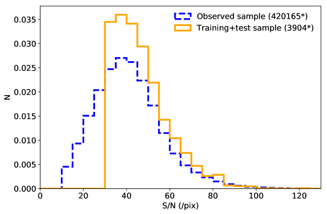
Figure 1: Normalised distribution of S/N  of RAVE DR6 spectra in the observed sample (blue dashed line, $420\,165$ stars) and in the training and test samples (solid orange line $3\,904$ stars in common between RAVE DR6 and APOGEE DR16).

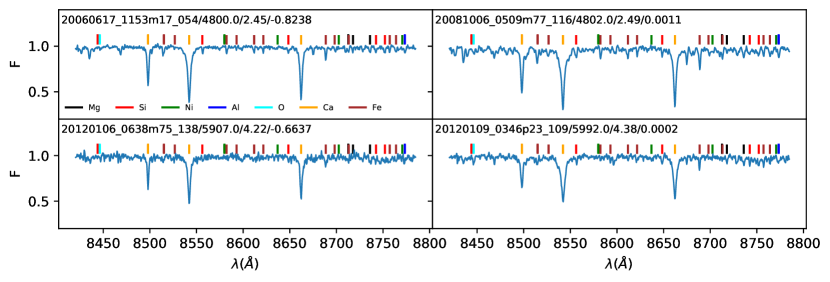
Figure 2: Example of four typical metal-poor and metal-rich dwarfs and giants RAVE spectra from the training sample. The RAVE_OBS_IDs and the atmospheric parameters are indicated in the top left corner of each panel. Apart from the prominent CaII triplet lines, the RAVE spectra also show a variety of more subtle spectral features (main chemical abundance diagnostic lines are over-plotted).

2 Training sample

One of the main goals of this study is to show that high-resolution stellar labels can be used to deduce atmospheric parameters and chemical abundances from lower resolution spectra. For this purpose, we need to build a training set that contains the labels - namely, the parameters we wish to derive (in our case, the atmospheric parameters and chemical abundances) and the observables (the spectra and photometric measurements). Here, we chose to work with labels provided by the APOGEE survey and observables from the RAVE spectroscopic survey, complemented by 2MASS (Skrutskie et al. 2006), Gaia DR2 (Gaia Collaboration et al. 2018a), and ALL_WISE photometry (Wright et al. 2010) as well as Gaia DR2 astrometry (Lindegren et al. 2018). Since the APOGEE survey, on average, offers higher resolution and higher signal-to-noise ratios (S/N) than the RAVE survey, we can translate the higher quality of the derived APOGEE labels to RAVE.

We take advantage of the latest release of APOGEE, namely, DR16 (Ahumada et al. 2020; Jönsson et al. 2020), which provides high-quality atmospheric parameters and chemical abundances. The APOGEE spectra are taken at near-infrared wavelengths with high resolution ($R=22\,500$ and $\lambda\in[1.5-1.7]\mu$m). The RAVE DR6 spectra have a spectral resolving power of $R\sim 7\,500$. We re-sampled the spectra to a common wavelength coverage of $\lambda\in[8\,420-8\,780]$Å, with equally spaced 0.4Åpixels.

We performed a cross-match based on the Gaia DR2 Source IDs between the $518\,387$ RAVE DR6 observations and the $473\,307$ observations of APOGEE DR16, resulting in a sample of $\sim 7\,000$ sources. In order to build a clean and coherent training sample based on APOGEE stellar labels and RAVE spectra, we cleaned this cross-matched sample in the following way.

Firstly, we required that a given star has available measurements of $\textit{T}_{\text{eff}}$, $\text{log}(\textit{g})$, $[\text{M}/\text{H}]$, $[\text{Fe}/\text{H}]$, $[\alpha/\text{M}]$, $[\text{Mg}/\text{Fe}]$, $[\text{Si}/\text{Fe}]$, $[\text{Al}/\text{Fe}]$, $[\text{Ni}/\text{Fe}]$ and their associated errors in the APOGEE set. We excluded parameters for stars with S/N_APOGEE¡60 (per pixel) and required the ASPCAP parameterisation flag to be aspcap_flag=0. The mean APOGEE $S/N$ of the sample is 420 per pixel. We filtered stars with a bad flag on chemical abundances, that is, selecting only X_Fe_FLAG=0. The ASPCAP pipeline uses spectral templates for matching any observations. Such procedures can lead to systematics (due for example to incomplete line list) that will be transferred by the CNN.

Secondly, we adopted the normalised, radial-velocity-corrected spectra from the DR6 of RAVE. The normalisation has been performed by the RAVE survey, with an iterative second-order polynomial fitting procedure (see Steinmetz et al. 2020b for more details). We required that the spectra have at least S/N¿30 per pixel. We excluded spectra showing signs of binarity or continuum issues (’c’, ’b’, and ’w’ according to the RAVE DR6 classification scheme, see Steinmetz et al. 2020b).

Finally, as detailed in Sect 3.2, we used absolute magnitudes during the training process. We required that a star have an apparent magnitude available in the 2MASS $JHK_{s}$, ALL_WISE W1&2 pass-bands, and Gaia DR2 $G$, $G_{BP}$ $G_{RP}$, and Gaia parallaxes (with parallax errors $e_{p}<15\%$). As such apparent magnitudes can suffer from dust extinction, we took advantage of the StarHorse catalogue, which provides improved extinction measurements based on RAVE and Gaia DR2 data (Queiroz et al. 2020, see also Santiago et al. 2016; Queiroz et al. 2018 for details on the method). We required that all spectra have an available StarHorse extinction ($A_{V}$).

The resulting common sample between APOGEE DR16 and RAVE DR6 consists of $3\,904$ high-quality RAVE spectra and high-quality atmospheric parameters and chemical abundances. The RAVE S/N distribution of this sample is presented in Figure 1. We carefully checked the spectra of the $3\,904$ stars of the sample in order to reject any misclassified stars, possibly having a very low S/N. Some examples of RAVE spectra are presented in Figure 2, for typical metal-poor and metal-rich dwarfs and giants. Kiel diagrams of the $3\,904$ targets based on APOGEE DR16 parameters are presented in the left panels of Figure 7.

3 Training the network

An artificial neural network consists of several layers of neurons that are interconnected. The strength of connections between the neurons is governed by the weight of each connection. This feature enables the network to translate the input data vector to the desired output labels. The weights need to be set to values with which the translation becomes meaningful. For example, a stellar spectrum sampled at $N$ wavelength points is fed into a neural network with $N$ input neurons and the network produces an output in the form of, for instance, effective temperature. The setting of weights is done through training. This is a process of passing a limited set of data vectors through the network and gradually adjusting the weights so that the output matches the pre-determined labels of the data vectors. Each passing of the input data and adjustment of the weights is known as an epoch and many epochs are needed to successfully train the network. Once this is done, a new data vector can be passed through the network and we obtain its label as a result. We note that convergence is reached when the error from the model has been sufficiently minimised. In theory, it could be the case that the desired level of error minimisation is never reached and the network would run indefinitely. We detail in Sect. 3.3 how we stop the training in such cases.

3.1 Architecture of the CNN

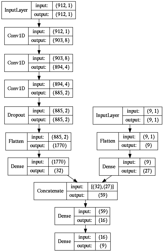
Figure 3: Representation of the architecture of the Keras model used in this study. The input layer (the spectra) is passed through three steps of convolution (Conv1D). Then, we randomly drop 20% of the neurons at each epoch of training with the dropout layer in order to prevent overfitting. We then flatten the output for the next dense layer (also called a fully connected layer). As an additional input, we include eight absolute magnitudes (2MASS $JHK_{s}$, ALL_WISE W1&2, and Gaia DR2 $G$, $G_{BP}$ $G_{RP}$ passbands) and one $A_{V}$ correction (input layer with shape of 9). We concatenate it to the main part of the network in the form of 27 neurons. The fully connected part of the network is then composed of two dense layers. The output is an array of nine parameters (atmospheric parameters and six chemical abundances).

In Figure 3, we present the architecture of the neural network used in this study. It is composed of three convolutional layers and two fully connected or dense layers. In the subsection below, we justify the reason for utilizing these features. We used the Keras python libraries for coding the network (Chollet et al. 2015). The stellar labels are normalised, ranging from 0 to 1 by using a Min-max normalisation.

3.1.1 Convolution and dense layers

Convolution layers are the key for detecting patterns and features in images (see e.g. Ciresan et al. 2011 for more details on this topic). In the present study, we work with one-dimensional normalised stellar spectra characterised by spectral line features. Such spectral features are indicators of the physical properties of the stars (temperature, gravity, chemical composition, etc). The ability to capture the relations between the different wavelength pixels in a spectrum, as opposed to treating them as independent entities, is the key to improved performance and this is provided by the convolutional layers.

To understand the impact of these types of layers we experimented with training our network with and without the convolution stage. In comparison to the network with the convolution stage, the training phase to find a stable solution is three to four times longer for the non-convolutional network. In addition to a lengthier training period, the output parameters are not recovered as precisely. This applies in particular to chemical abundances. After trying many different layouts, we adopted a network with three convolution layers that contain eight, four, and two filters, respectively (as shown in Figure 3). We adopted a kernel size of ten pixels for all three layers. Tests revealed that kernel sizes between 5 to 20 pixels tend to extract features efficiently. Much larger kernels (¿40 pixels) degrade the performance.

Between the convolution layers and the fully connected part of the network, we used a dropout layer that ensures that a certain randomly chosen fraction of the neurons are not used at each of the epochs during the training phase. This type of regularisation prevents the over-fitting the network and also prevents the algorithm from relying on a smaller part of the network alone. We tested a range of fractions from 10 to 30%, with no major change in the training phase. We adopted 20% for the final analysis.

The fully connected layers (also called ’dense’ layers) following the convolutional stage are a more common type of neural network layers. They receive the output of the convolutional stage in the form of learned spectral features and convert them to the output labels (atmospheric parameters, abundances) that are sought. We must allow enough complexity in the network at this stage for it to be able to model the non-linear relations between features and labels. We adopted the Leaky Rectified Linear Units (Leaky ReLU) activation function instead of Rectified Linear Units (ReLU), allowing us to face the dead ReLU problem (i.e. null or negative ReLU leading to no learning in the layers below the dead ReLU). We are, thus, less sensitive to the initialisation of the network.

3.1.2 Initialisers and cost function

The weights of the CNN must be initialised prior to the training. The choice of how we initialise them can influence the performance of the network. We adopted the default initialiser for our convolution and dense layers, namely, the ’glorot_uniform’ and the default bias initialiser, ’zeros’, meaning that the weights prior to training are drawn from a uniform distribution within a certain range.

To train the network, we need a cost function that evaluates how good the network’s performance is at each iteration and which would also allow us to compute the gradient in the weight space so the difference between the output and pre-determined labels can be minimised. The choice of this function is important. We experimented with a simple mean-squared error loss-function and a negative log-likelihood criterion. Tests performed on the negative log-likelihood criterion revealed that such a criterion appears to be inferior for our science case, and it adds too much complexity to the framework.

3.1.3 Effect of noise in the training phase

The training and test samples include in total $3\,904$ stars with $S/N>30$ per pixel. As a test, we constrained this range to $S/N>40$ ($2\,529$ stars) and $S/N>50$ ($1\,289$ stars). With a lower number of stars, the performance naturally tends to degrade. We believe, however, that this lack in performance is only due to the fact that we have a limited common sample with APOGEE. In general, high $S/N$ data and sufficient statistics lead to a better training phase, but lower $S/N$ spectra also come with a higher degree of correlated noise, which the network is likely to learn.

As another check, we extended the $S/N$ range to $S/N>20$, $S/N>15$ and $S/N>10$ per pixel, leading to $4\,802$, $5\,023$, and $5\,136$ stars in the training sample. We concluded that including such low-$S/N$ data in the training phase tends to reduce the quality of the training and degrades the overall performance.

We tried to train a network with a sample composed only of stars with $S/N<30$, finding that no robust solution could be reached, probably owing to to the spectral information being too hidden by noise. Especially for the chemical abundances, the network is unable to reproduce the main Galactic trends and basically fits a straight line in the $[\alpha/\text{M}]$ versus $[\text{M}/\text{H}]$ plane instead of reproducing the $\alpha-$rich and $\alpha-$poor sequences. A similar finding also holds for other elements. Our conclusion is that an efficient training cannot be performed if only low $S/N$ stars are present in the training set.

We recommend that for future spectroscopic surveys particular attention should be given when defining the training sample $S/N$ range, because too low $S/N$ spectra lead to worse training and performance for the CNN.

3.2 Feeding absolute magnitudes to the neural network

In addition to spectra, our input includes broad-band photometry. Absolute magnitudes provide strong constraints on the effective temperature and the surface gravity of a star. We adopted the 2MASS apparent magnitudes $m$ in the passbands $JHK_{s}$ (1.235, 1.662, and $2.159\,\mu$m, respectively), ALL_WISE W1 and W2 pass-bands (3.4, and $4.6\,\mu$m) and Gaia DR2 $G_{BP}$ (328.3-671.4 nm), and $G_{RP}$ (629.6-1 063.7 nm) and $G$ (332.1-1 051.5 nm) bands, using the cross-matches provided in RAVE DR6 (Steinmetz et al. 2020b). The distributions of these apparent magnitudes are shown in Figure 4.

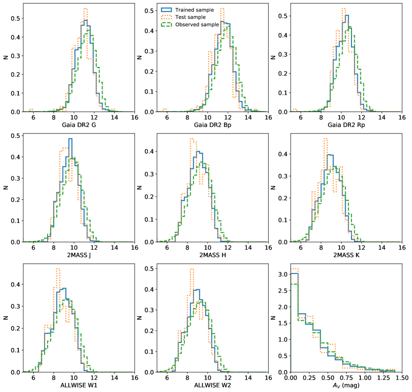
Figure 4: Normalised distribution of Gaia, 2MASS, ALL_WISE apparent magnitudes and extinction ($A_{V}$) for the training sample (blue, solid), the test sample (orange, dotted), and the observed sample (green, dashed). Those magnitudes are converted to absolute magnitudes and are used during the training phase.

We computed absolute magnitudes, $M,$ using the parallaxes ($p$) from the second data release of the Gaia satellite (Gaia Collaboration et al. 2018b), using $M=m+5\times[\log_{10}(p)+1]$. We selected the best measurements for which we required the errors on the parallax, $e_{p}$, to be better that $20\%$ (96.5% of the spectra of the initial cross-match with APOGEE DR16 fulfil this criterion). We discuss the performances of the CNN parameterisation for stars with parallax errors larger than $20\%$ in Appendix A.

As stellar magnitudes can suffer from dust extinction even in the infrared passbands, we adopted the extinction correction $A_{V}$ from StarHorse (see Queiroz et al. (2018); Anders et al. (2019) for more details). The distributions of $A_{V}$ for the training, test, and observed sample are presented in Figure 4. We find that 78% of our stars have an extinction lower than $A_{V}=0.5$ mag. Our tests found that stars with $A_{V}>0.8$ show a smaller error in $\textit{T}_{\text{eff}}$ by 20 K if we include this correction.

Our choice to compute absolute magnitudes from parallaxes instead of, for example, StarHorse distances was motivated by the fact that we want to restrict our model dependency as much as possible. As a test, we computed absolute magnitudes using StarHorse distances, but no notable difference in the training was measured.

The eight absolute magnitudes and the extinction corrections were then added smoothly to the CNN architecture, directly in the fully connected part, as 27 neurons (see scheme in Figure 3). We tested several layer sizes for this part: below 27, the performances tended to degrade and above 27, no further improvement was notable. We note that we did not directly apply the $A_{V}$ correction to the absolute magnitudes, thus leaving the network with more flexibility to learn from it.

It has been shown that Gaia DR2 astrometric measurements have small systematic errors, in particular, an offset of the parallax zero-point that varies across the sky. This parallax zero-point offset is dependent on magnitude and colour (Lindegren et al. 2018; Arenou et al. 2018). This offset is roughly of the order of 50 $\mu\text{as}$. Following the way we compute our absolute magnitudes, this parallax offset translates into a shift of the order of 0.01 magnitudes. In the context of this study, this offset is negligible. We refer the reader to Sect. 7 for a discussion on the advantage of adding photometry during the training process.

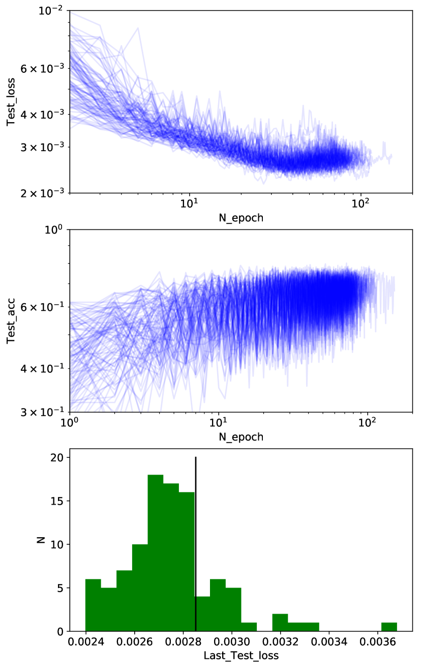
Figure 5: Top: Value of the cost function for the test sample (Test_loss) for the 100 CNN runs as a function of the epoch. Middle: Accuracy computed on the test sample (Test_acc) as a function of the epoch. Bottom: Distribution of 100 values of Test_loss after the training was completed. Vertical black line indicates the 80th percentile of the distribution.

3.3 Training an ensemble of 100 CNNs

From the quality cuts and selection process detailed above, our starting sample is thus composed of $3\,905$ stars, with stellar labels corresponding to atmospheric parameters and chemical abundances. Before training the CNN, we split the data into a training sample and a test sample, as is a common practice in the machine-learning community. We adopted a fraction of 6% for the test sample to retain a large the training sample. This led to $3\,669$ stars in the training sample and 235 stars in the test sample. We tested several test and training fractions, from 3 to 40%, with no major difference in terms of training. In order to provide stable results and errors, we built an ensemble of 100 trained CNNs, all of them initialised differently. A similar method was recently used by Bialek et al. (2020).

One challenge while using a CNN is to stop the learning phase at the right time. The model can under-fit the training and test samples in case of insufficient training. On the other hand, in cases of over-fitting, the training sample will perfectly fit the model, but the performances on the test sample will degrade drastically (which is the main reason behind the training-test split). One solution is to stop the training phase when the performance on a validation dataset starts to degrade. In this context, we adopted the commonly used early-stop procedure. If after 40 epochs (the so called patience period), the solution does not improve, we stop the training. We tried different levels of patience, finding that 40 epochs provide the best compromise between final accuracy and computation time.

Typical curves of the cost functions ’Test_loss’ for the test sample are presented in Figure 5 for the 100 runs, as well as the accuracy Test_acc. It is clear that the training phase takes no more than 120 epochs. Training the CNN takes between 70 to 90 seconds per run. We can also see that the last value of the cost function of the test sample (Last_Test_loss) can vary from one run to another. We plot such values in the bottom panel of Figure 5. We excluded networks with too large a value of Last_Test_loss (everything inside of the lower 20th percentile of the distribution).

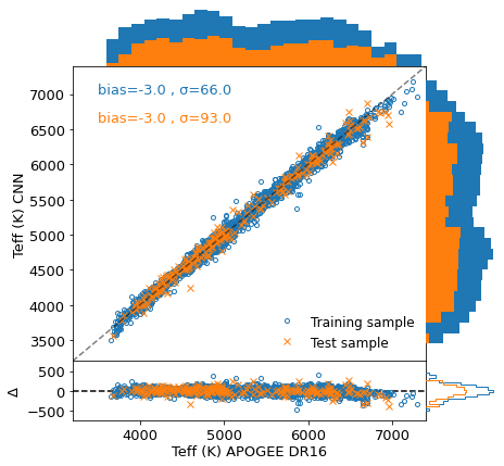
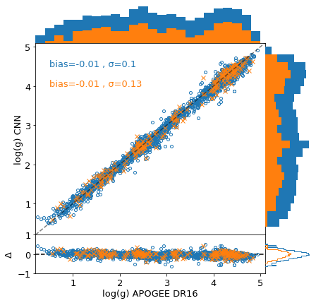
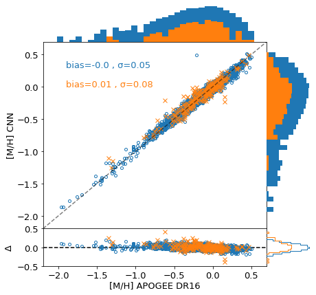
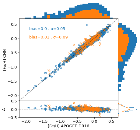
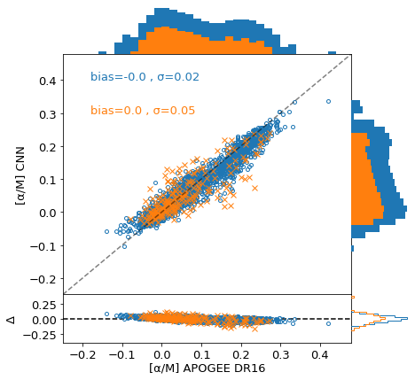
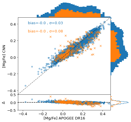
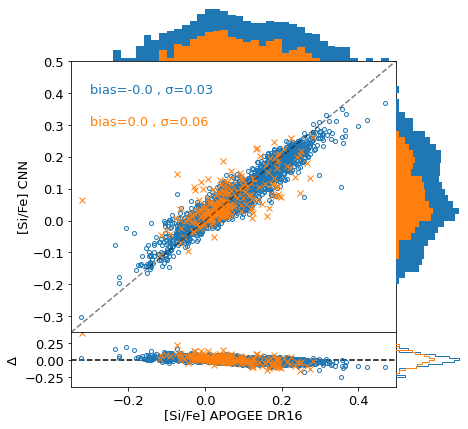
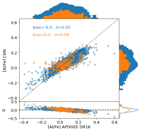
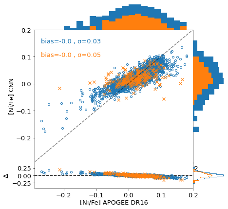
Figure 6: One-to-one relation between the CNN trained labels (y-axis) and the input labels (x-axis, APOGEE DR16 data). The training sample is plotted with blue circles, while the test sample is shown with orange crosses. The x- and y-axis parameters are presented as histograms with a logarithmic scale. For each parameter, a typical mean difference and scatter are computed in both sets. We plotted the difference $\Delta$ between the CNN trained labels and the APOGEE DR16 input labels with the same symbols and colours, and its histogram with a logarithmic scale.

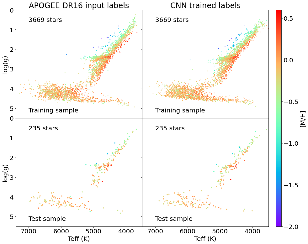
Figure 7: Top left: Kiel diagram of the APOGEE DR16 stars (used in the training sample), colour-coded with overall $[\text{M}/\text{H}]$. Top right: For the same stars, trained labels, averaged over 80 trained CNN. Bottom left: APOGEE DR16 parameters of the test sample. Bottom right: Trained labels, averaged over 80 trained CNN, for the same test sample. The right panels correspond to what the network learns from the APOGEE parameters (left panels).

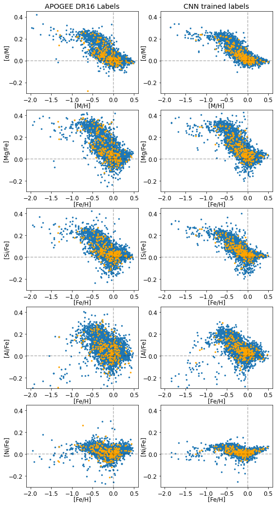
Figure 8: Left panels: Abundance patterns of the APOGEE DR16 labels used as input for our CNN, for the training sample (blue) and for the test sample (orange). Right panels: Abundance patterns of the averaged labels trained over 80 CNNs.

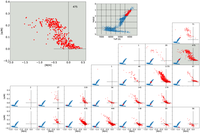
Figure 9: Averaged trained abundance patterns $[\alpha/\text{M}]$ vs. $[\text{M}/\text{H}]$ for the training sample (red dots). Trends are shown for sub-samples in $\textit{T}_{\text{eff}}$ (500 K bins) and $\text{log}(\textit{g})$ (1 dex bins) shown as in-set Kiel diagrams, where the overall stellar distribution is plotted in blue with the selected subsample highlighted in red. The number of stars is indicated in the top right corner of each panel.

3.4 Result of the training

In Figure 6, we compare the labels used as input of our CNN (from APOGEE DR16) to those trained by the network (averaged over the 80 runs). The network is able to learn a significant amount of information about the main atmospheric parameters $\textit{T}_{\text{eff}}$, $\text{log}(\textit{g})$, $[\text{M}/\text{H}]$ as well as $[\text{Fe}/\text{H}]$. No obvious systematic trends are visible while the dispersion is low, for both training and test samples. The mappings of $\textit{T}_{\text{eff}}$ and $\text{log}(\textit{g})$ are very similar between the training and test samples, as seen in the distributions. Abundances $[\alpha/\text{M}]$, $[\text{Si}/\text{Fe}]$, $[\text{Mg}/\text{Fe}]$, $[\text{Al}/\text{Fe}]$ and $[\text{Ni}/\text{Fe}]$ compare well with the input labels. Because of the poor mapping of the parameter space, the stars with very low or very high abundance ratios can suffer from systematic trends, especially in the metal-poor regime. It is, for example, visible for the [Al/Fe]-poor tail. In general, the dispersion in the test sample is similar to the one in the training sample, indicating that we do not over-fit our data. Finally, we note that for $[\text{Al}/\text{Fe}]$ and $[\text{Ni}/\text{Fe}]$, the comparison with the input APOGEE DR16 labels does not track the 1-to-1 relation, even for the bulk of the data, meaning that the model predicted during the training could suffer from systematic trends for those two elements. In general, we warn the reader that systematics a low S/N, typically $S/N<30$, can be present in the data. The abundances for those stars should be thus used with caution.

In Figure 7, we present a Kiel diagram of $\textit{T}_{\text{eff}}$ and $\text{log}(\textit{g})$ from the training sample (left columns), for the training (top) and test (bottom) samples. In the right columns, we present the labels as trained by the CNN. The main features in the Kiel diagram are well recovered in both training and test samples: the position and inclination of the red clump, the giant branch with a smooth metallicity sequence, the turn-off sequence. The sequence of the very cool dwarfs spans a large $\textit{T}_{\text{eff}}$ range, and shows low scatter even in the very cool regime.

In the left panels of Figure 8, we present the abundance patterns used as input for our CNN, for both training and test samples. We recall that those labels ($[\text{Fe}/\text{H}]$, $[\alpha/\text{M}]$, $[\text{Si}/\text{Fe}]$, $[\text{Mg}/\text{Fe}]$, $[\text{Al}/\text{Fe}]$, $[\text{Ni}/\text{Fe}]$) are derived by APOGEE DR16. In the right panels, we present the labels as trained by our CNN, averaged over 80 runs. The chemical patterns of the trained labels, in particular $[\text{Al}/\text{Fe}]$, show slightly less scatter than the original labels (around 0.05 dex). This effect comes mainly from the fact that during the training, the neural network values tend to stay within the boundaries of the data. In spite of the poor mapping of the parameter space in the metal-poor regime, the network is still able to provide robust output in that metallicity regime.

In Figure 9, we present the averaged $[\alpha/\text{M}]$ ratios of the training sample, as a function of $[\text{M}/\text{H}]$, for different bins of $\textit{T}_{\text{eff}}$ and $\text{log}(\textit{g})$. One can see that the $[\alpha/\text{M}]-$rich sequence is mainly composed of red giant branch stars, while only a few stars are dwarfs. Similar plots are presented in Appendix D for $[\text{Mg}/\text{Fe}]$, $[\text{Si}/\text{Fe}]$, $[\text{Al}/\text{Fe}]$, and $[\text{Ni}/\text{Fe}]$.

4 Estimation of atmospheric parameters and abundances of RAVE DR6 spectra

In this section, we provide details of the way we built an observed sample of stars based on RAVE DR6 spectra, then we present the predicted atmospheric parameters and chemical abundances of this observed sample.

4.1 Creation of the observed sample

Our observed sample is based on RAVE DR6 normalised radial-velocity-corrected spectra (Steinmetz et al. 2020b). We required that a spectrum have ALL_WISE W1&2, 2MASS $JHK_{s}$ photometry and Gaia DR2 $G$, $G_{BP}$, $G_{RP}$ bands available as well as its Gaia DR2 parallax (no cut on parallax errors). We checked that all spectra have StarHorse extinction measurements ($A_{V}$, Queiroz et al. 2020). Finally, we restricted our observed sample to a range of S/N¿10 per pixel (as determined by RAVE DR6), removing stars with problematic spectra (”c” and ”w” according to the RAVE DR6 classification). This leads to an observed sample composed of $420\,165$ stars with $S/N>10$ per pixel. The S/N distribution of the observed sample is presented in Figure 1.

Adopting the orbital data from Steinmetz et al. (2020a), we carefully checked that both the training and observed samples probe the same Galactic volume, in terms of mean Galactocentric radii and height above the Galactic plane. Also, as the stellar age distribution can vary from one sample to another we took advantage of the StarHorse ages of Queiroz et al. (2020) to check the age distributions of both the training and observed samples. The age distributions cover the same range and their shapes are consistent. Tests performed with BDASP ages from Steinmetz et al. (2020a) have led to the same conclusion.

4.2 Prediction of atmospheric parameters and abundances

Once a given CNN is trained, we can predict atmospheric parameters and chemical abundances for the entire observed sample. Predicting nine parameters for $420\,165$ stars is quick, lasting ten seconds on a simple GPU unit. Thus, estimating parameters for 80 CNN runs does not take more than 15 minutes. We then computed a set of parameters averaged over the 80 runs, as well a typical dispersion used as error (see Sect. 5).

4.2.1 Atmospheric parameters

In Figure 10, we present a Kiel diagram of the observed sample, sliced in S/N, for $371\,967$ stars with $S/N>20$ per pixel, and parallax errors better than $20\%$. We plotted such a diagram in two different fashions: colour-coded with overall metallicity, and normalised-density map. For such a plot, we selected normal and hot stars (’n’ and ’o’) according to the RAVE DR6 classification scheme (Steinmetz et al. 2020b).

At low S/N, we recover the main features of a typical Kiel diagram, especially the cool main sequence and the location of the red clump. The bottom of the cool main sequence shows a gradient in metallicity, while the turn-off shows no clear gradient. For very high S/N, the cool dwarf sequence is very narrow, while the red giant branch shows a slight warp as in the training sample. At low temperatures ($\textit{T}_{\text{eff}}<4300\,K$), we are able to properly characterise giants and dwarfs, putting them on the right sequence, with no degeneracy observed.

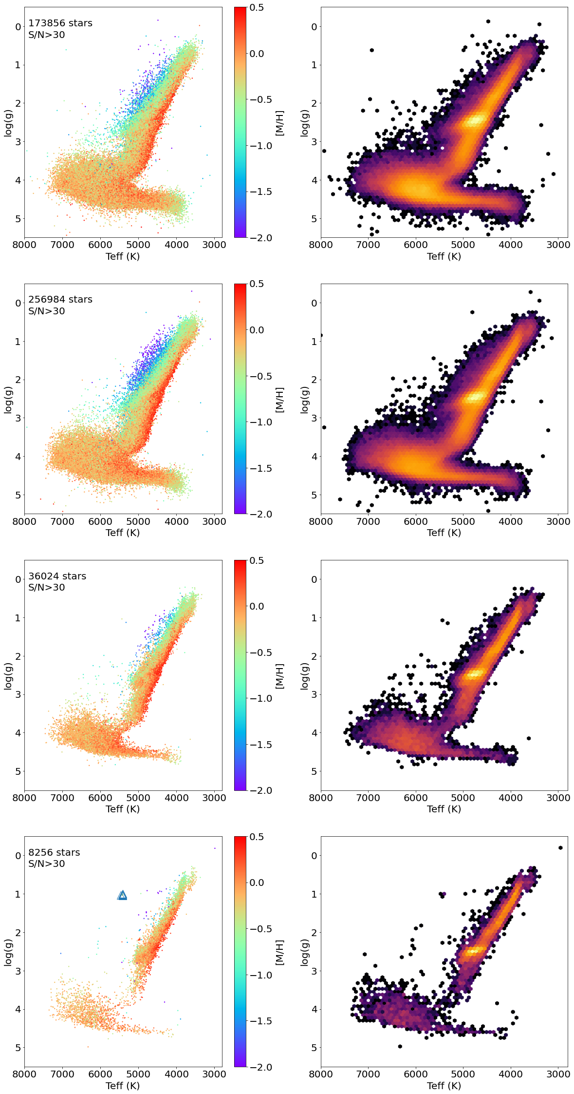
Figure 10: Kiel diagram of $371\,967$ stars of the observed sample, sliced in S/N, colour-coded by $[\text{M}/\text{H}]$ (left column) and plotted as a normalised density map (right column). Only stars with ’n’ and ’o’ classification (normal and hot stars), and parallax errors better than $20\%$ are plotted. The main features of the Kiel diagram are well recovered in the observed sample. The 6 blue triangles in the bottom panel correspond to the yellow supergiant Gaia ”5983723702088571392”, discussed in Section 6.6.

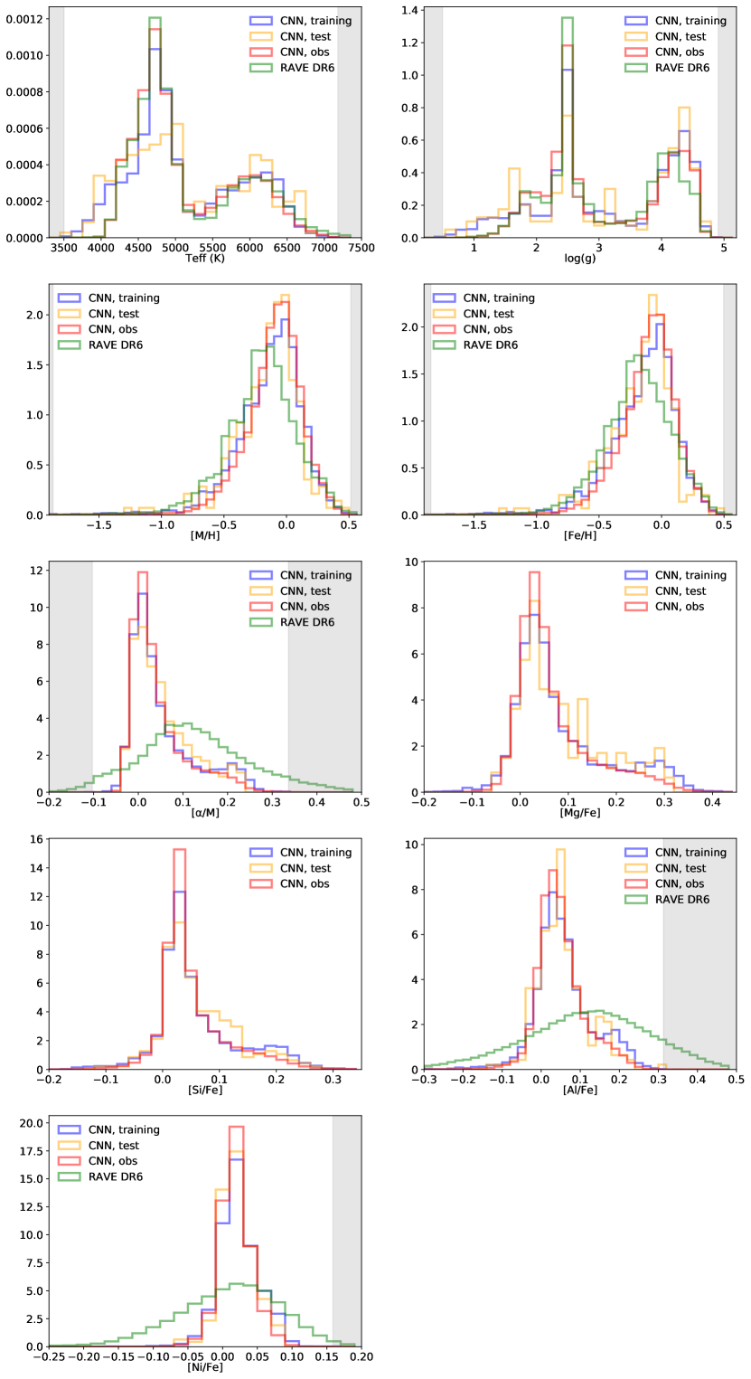
Figure 11: Normalised distribution of atmospheric parameters and abundances in the training sample (blue), in the test sample (yellow), and the observed sample (red). For the same stars of the observed sample, we show a normalised distribution of the corresponding RAVE DR6 parameters (taken from Steinmetz et al. (2020a)). The grey areas define the zones outside the limits of the training sample parameters space.

In Figure 11, we present normalised distributions of $\textit{T}_{\text{eff}}$, $\text{log}(\textit{g})$, $[\text{M}/\text{H}]$, and $[\text{Fe}/\text{H}]$ of the training, test, and observed sample, for $S/N>40$. We also added distributions of RAVE DR6 parameters for the same stars (with algo_conv_madera=0, corresponding to the best solutions, see Steinmetz et al. 2020a for more details). We first see that the training and test sample distributions tend to track each other very well and that the observed sample is well defined in the training and test sample limits (defined by the grey areas). The same behaviour is observed for $[\text{Fe}/\text{H}]$, because APOGEE DR16 $[\text{Fe}/\text{H}]$ and $[\text{M}/\text{H}]$ tend to track very well each other (Jönsson et al. 2020). Both $\textit{T}_{\text{eff}}$ and $\text{log}(\textit{g})$ from RAVE DR6 track pretty well the CNN distributions. In addition, both RAVE DR6 $[\text{M}/\text{H}]$ and $[\text{Fe}/\text{H}]$ present a metallicity-dependent shift with respect to our study, varying basically for zero in the metal-rich regime to roughly 0.1 dex in the metal-poor regime. It is a known systematic shift between RAVE DR6 and APOGEE DR16; see, for example, Figure 22 in Steinmetz et al. (2020a).

4.2.2 Individual chemical abundances

In Figure 12, we present abundance patterns for $[\alpha/\text{M}]$ as a function of the overall metallicity $[\text{M}/\text{H}]$. We selected $301\,076$ stars with S/N¿30 per pixel, RAVE DR6 ‘n&o’ classification (’normal’ and ’hot’ stars) and parallax errors lower than $20\%$. In order to disentangle the different stellar classes, we decomposed our sample in bins of 500 K in $\textit{T}_{\text{eff}}$, and 1 dex in $\text{log}(\textit{g})$, and present the $[\alpha/\text{M}]$ vs. $[\text{M}/\text{H}]$ trends for different locations in the Kiel diagram (see Appendix D for similar plots with $[\text{Si}/\text{Fe}]$, $[\text{Mg}/\text{Fe}]$, $[\text{Al}/\text{Fe}]$, and $[\text{Ni}/\text{Fe}]$.)

Dwarf stars exhibit typical low-$[\alpha/\text{M}]$ sequences, while giants populate both the low-$[\alpha/\text{M}]$ and high-$[\alpha/\text{M}]$ range up to halo chemistry. Red clump stars show a smooth transition from the low- to the high-$[\alpha/\text{M}]$ regime, with a strongly decreasing density. On the other hand, in the range of $4000<\textit{T}_{\text{eff}}<4500\,$K and $1<\text{log}(\textit{g})<2$, the high-$[\alpha/\text{M}]$ regime is clearly marked by a continuum of stars from solar-$\alpha$ up to 0.25 dex. Such behaviour is also observed when plotting $[\text{Si}/\text{Fe}]$ and $[\text{Mg}/\text{Fe}]$ as a function of $[\text{Fe}/\text{H}]$ (see Appendix D).

We note that the low-metallicity high-$[\alpha/\text{M}]$ plateau shows different behaviours in different regions of the Kiel diagram. This is mainly driven by the fact that we only have a few stars for $[\text{M}/\text{H}]<-1\,$dex in the training sample, showing quite different trends. For future machine-learning applications, we should put substantial efforts into properly mapping the parameter space when creating a training sample. The case of $[\text{Al}/\text{Fe}]$ is discussed in Appendix D.

We have shown that in using a CNN approach and high-resolution stellar labels, we are able to provide reliable $[\alpha/\text{M}]$ values for more than $301\,076$ stars, thus extending the scientific output of RAVE spectra beyond RAVE DR6.

In Figure 11, we present normalised distributions on CNN chemical abundances in the training, test, and observed sample, as well as the corresponding values from RAVE DR6 ($[\alpha/\text{Fe}],[\text{Al}/\text{Fe}],[\text{Ni}/\text{Fe}]$, Steinmetz et al. 2020a). We first note that both training and test sample distributions show basically the same shape. For $[\text{Mg}/\text{Fe}]$, the bi-modality is not well represented in the test sample, because of a larger scatter in $[\text{Mg}/\text{Fe}]$ at a given $[\text{Fe}/\text{H}]$. As for the atmospheric parameters, the chemical abundances in the observed sample track pretty well the training and test sample, for this regime of S/N ($S/N>40$). We note that for lower S/N regimes, the distributions of the observed sample present larger tails than the training sample. Finally the $[\alpha/\text{Fe}]$, $[\text{Al}/\text{Fe}]$, and $[\text{Ni}/\text{Fe}]$ ratios from RAVE DR6 present broader distributions than the present study. Such an effect is already visible in Figure 22 of Steinmetz et al. (2020a), where RAVE DR6 and APOGEE DR16 are compared. The RAVE DR6 abundances show a larger scatter at a given metallicity, mainly because of lower spectra resolution. In the present study, besides the intermediate resolution of the RAVE spectra, our CNN is able to provide more precise abundances, showing narrower distributions. We compare further $[\alpha/\text{Fe}]$ ratios between our study and RAVE DR6 in Sect 6.5.

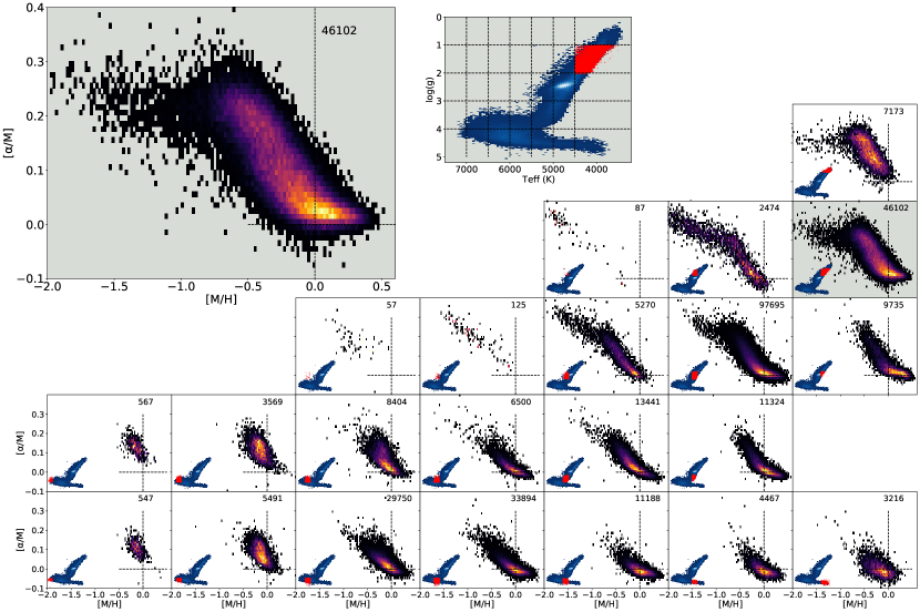
Figure 12: The $[\alpha/\text{M}]$ vs. $[\text{M}/\text{H}]$ for $301\,076$ stars of the observed sample with S/N¿30 per pixel, RAVE DR6 ’n&o’ classification, and parallax errors lower than $20\%$. The sample is presented in panels corresponding to cuts in effective temperature and surface gravity (steps of 500 K in $\textit{T}_{\text{eff}}$ and 1 dex in $\text{log}(\textit{g})$. For each panel, we overplotted a $\textit{T}_{\text{eff}}-\text{log}(\textit{g})$ diagram with the location of the plotted stars marked in red.

5 Determination of uncertainties

Despite the fact that we employ the same input labels in every run, the CNN does not provide the same trained labels because a new set of weights is automatically generated by the CNN during each run and the trained labels then change slightly. We showed the resulting average trained labels in Sect 3.4. Here we present the resulting errors (precision), defined as the dispersion of each label for the 80 runs. As a result, the errors in both test and observed samples are derived in the same fashion. In Figure 13, we present the error on our nine atmospheric parameters and abundances as a function of $\textit{T}_{\text{eff}}$, $\text{log}(\textit{g})$ and $[\text{M}/\text{H}]$, for $391\,035$ stars with $S/N>20$ per pixel. The uncertainty for the nine parameters tend to increase for both the hot and the cool tails. The same effect is visible for the stars with $\text{log}(\textit{g})<2$. On average, the dwarf stars tend to show larger errors than the giants. The uncertainties on the nine parameters tend to increase with respect to the bulk of errors for the metal-poor tail. In the same figure, we present normalised distributions of uncertainties for the observed sample, together with the training and test samples. Overall, the trained labels show on average smaller errors than the test and the observed sample, mostly because the training sample covers a higher S/N range. The test and observed sample tend to track each other well, meaning that we do not over-fit our model.

As a test, we added random offsets to the labels of the training sample, drawn from Gaussians with widths given by the quoted uncertainties from APOGEE DR16. We observed that the resulting error distributions barely change.

A recent study by Bialek et al. (2020) adopted a negative log-likelihood criterion instead of a mean squared error loss-function as employed in our study. In that way, they were able to derive the individuals error of the predicted atmospheric parameters. We explored such a criterion. Because of the limited number of stars in our training sample, this criterion did not provide improved results. We therefore kept a simple mean squared error loss-function and errors derived over several CNN runs.

The present uncertainties reflect, in fact, the internal dispersion of the CNN. Figure 13 shows that the method is internally precise and stable if we consider such types of series of trainings (Monte-Carlo type). As a consequence, such uncertainties could be then underestimated, with respect to typical external errors that we would expect at such a resolution. Typical external errors for classical pipelines using RAVE spectra report errors of roughly 100K in $\textit{T}_{\text{eff}}$, 0.15-0.2 dex in $\text{log}(\textit{g})$, and 0.10-0.15 dex in metallicity and chemical abundances (see for exemple Steinmetz et al. 2020a). However, as presented in Figure17, we note that the dispersion in atmospheric parameters and abundances for a star with several RAVE observations is very compatible with the uncertainties derived with our method.

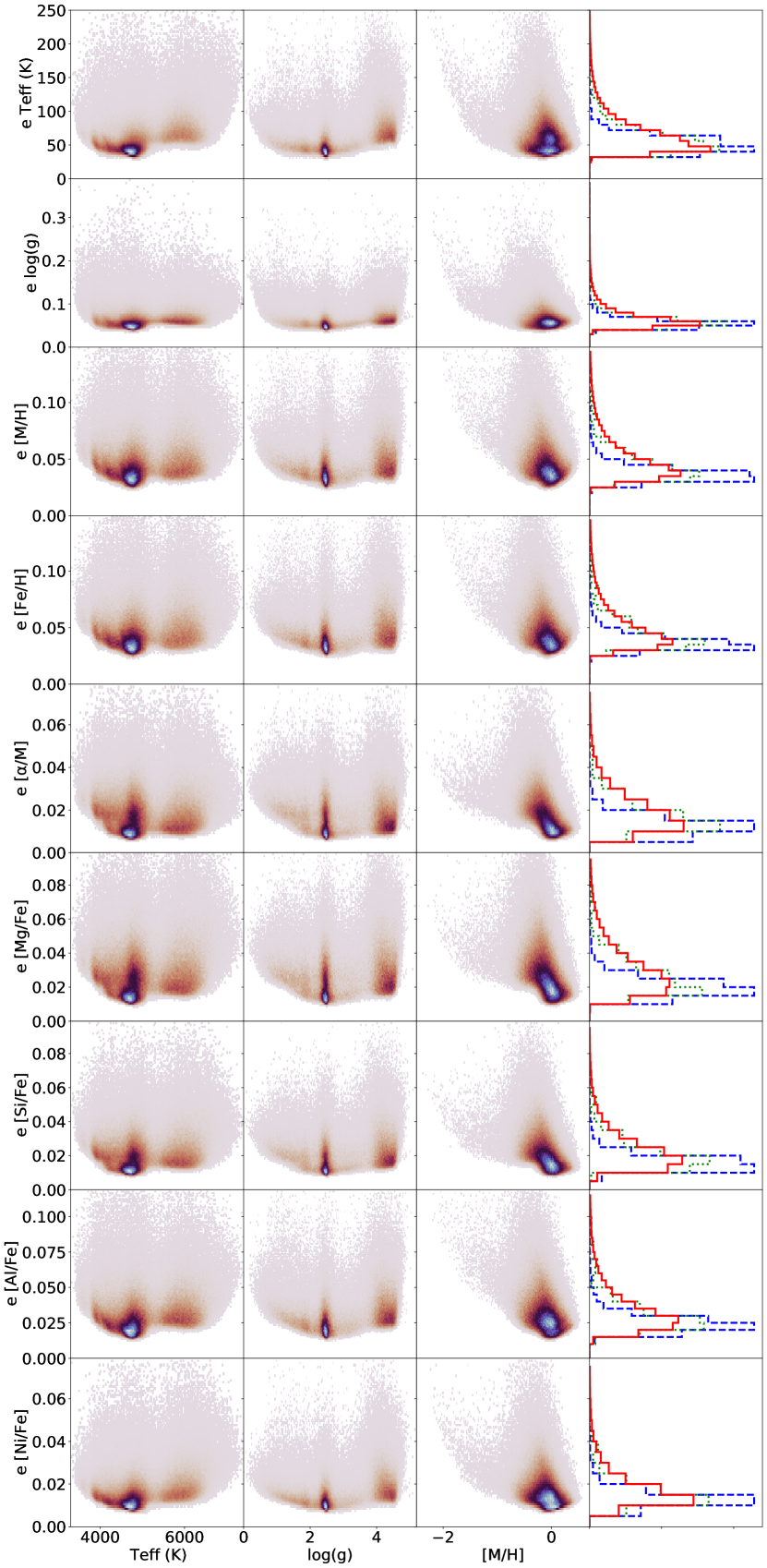
Figure 13: Errors of atmospheric parameters and chemical abundances plotted as a function of $\textit{T}_{\text{eff}}$, $\text{log}(\textit{g})$ and $[\text{M}/\text{H}]$ for $391\,005$ stars of the observed sample. We also present normalised distribution of errors in the trained labels (blue, dotted), the test sample (green, dashed), and the observed sample (red, solid).

Machine-learning methods are, within limits, able to extrapolate and provide parametrisations for stars outside the boundaries of the training sample parameter space. Together with individual uncertainties on the parameters and abundances, we provide individual flags for such stars. As an example, a star parametrised with an effective temperature inside the training sample space will have flag_teff=0, while the flag will be equal to 1 if $\textit{T}_{\text{eff}}$ is outside that range. Stars with flags equal to 1 may suffer from systematics caused by extrapolation outside the training sample parameter space.

6 Validation of atmospheric parameters and abundances

In this section, we proceed to several comparisons with respect to external datasets in order to validate our atmospheric parameters and chemical abundances. We refer the reader to Appendix B for a comparison with stellar clusters and to Appendix C for a comparison of our CNN results with a sample of HR data.

6.1 Validation of surface gravities with asteroseismic data

The asteroseismology of stars with solar-like oscillations is now widely used in large spectroscopic surveys as an additional constraint since it ultimately calibrates the $\text{log}(\textit{g})$ measured from spectra (RAVE: Valentini et al. 2017; GES: Pancino & Gaia-ESO Survey consortium 2012; APOGEE: Pinsonneault et al. 2018; LAMOST: Wang et al. 2016; GALAH: Kos et al. 2017). For stars with solar-like oscillations, as well as red giants, $\Delta\nu$, the frequency at maximum oscillation power, is used for determining $\text{log}(\textit{g})_{\rm seismo}$ using only the additional parameter, $\textit{T}_{\text{eff}}$. The $\text{log}(\textit{g})_{\rm seismo}$ value depends very weakly on $\textit{T}_{\text{eff}}$, making this quantity reliable even for surveys affected by degeneracies such as RAVE (Kordopatis et al. 2011a, 2013).

The RAVE survey has some overlap with the fields observed by the K2 mission, the re-purposed Kepler satellite (Van Cleve et al. 2016). In Valentini et al. (2017), a first comparison (and consequent calibration) of the RAVE spectroscopic $\text{log}(\textit{g})$ with the seismic value was performed using 89 targets in K2-Campaign 1. Information on the RAVE-K2 sample, the reduction of the seismic data, and the calculation of the seismic $\text{log}(\textit{g})$ can be found in Valentini et al. (2017). In the first six Campaigns of K2, solar-like oscillations were detected for 462 red giants (Steinmetz et al. 2020a, Valentini et al, in prep.) and the seismic $\text{log}(\textit{g})$ was derived. Here, we compare these seismic $\text{log}(\textit{g})$ values with the values determined using our CNN.

Figure 14 shows that the labels (APOGEE DR16) and the K2 $\text{log}(\textit{g})$ values exhibit a tight and un-biased 1-to-1 relation (left panel, $\rm bias=-0.03$ dex and dispersion $\sigma=0.04$ dex). The K2 $\text{log}(\textit{g})$ values also agree well with the labels trained by the CNN (middle panel), with a slightly higher scatter ($\sigma=0.09\,$dex). Finally, in the right panel of Figure 14, we compare the predicted surface gravity for 433 common stars of our observed sample with K2 data, finding an very good agreement with a very small bias and a dispersion of 0.14 dex. We note that the $\text{log}(\textit{g})$ values from RAVE DR6 show a larger scatter with respect to K2 data than our CNN $\text{log}(\textit{g})$ values (see Figure 23 of Steinmetz et al. 2020b).

Keeping in mind that we are limited by the narrow spectral range of the RAVE spectra, those comparisons illustrate all the potential of a method based on CNN. A more detailed discussion on the impact of the use of photometry can be found in Sect. 7.

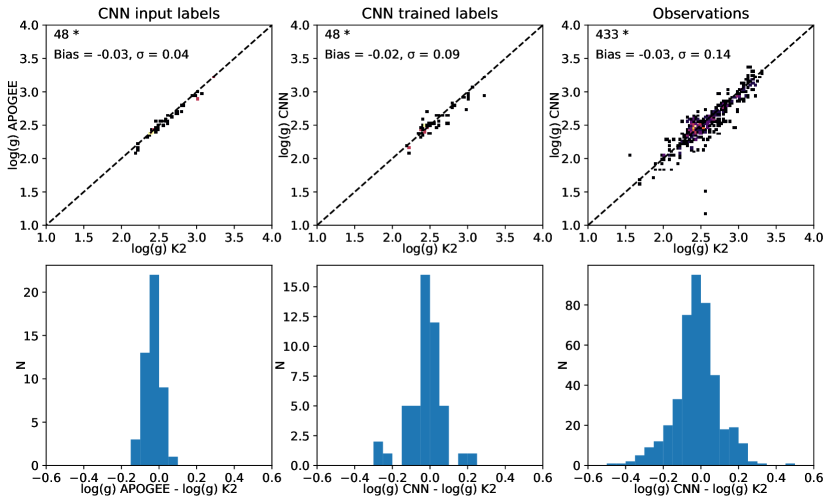
Figure 14: Comparison of surface gravities from the present study with K2 asteroseismic data. Left: Comparison with the $\text{log}(\textit{g})$ labels from APOGEE DR16 used as input by our CNN. Middle: Comparison with averaged labels trained by the CNN. Right: Comparison with averaged $\text{log}(\textit{g})$ predicted for common stars in the observed sample. Mean difference and scatter are indicated in the top left corner of each panel.

6.2 Comparison with RAVE DR6 BDASP $\text{log}(\textit{g})$

In the latest data release of RAVE (DR6, Steinmetz et al. 2020a), improved $\text{log}(\textit{g})$ estimates based on Gaia DR2 parallaxes and Bayesian isochrone fitting are provided, thanks to the BDASP pipeline (McMillan et al. 2018). This section is dedicated to comparing RAVE/BDASP surface gravities to those derived by our CNN in the present study.

The left panel of Figure 15 compares the input APOGEE DR16 $\text{log}(\textit{g})$ with those of BDASP . The dwarfs ($\text{log}(\textit{g})>3.5$) show a shift of about +0.1 dex, while the giants do not show any bias with respect to RAVE DR6. The typical dispersion is 0.14 dex for both types of stars with a bias of 0.05 dex. We notice that the surface gravities provided by APOGEE DR16 show a smaller dispersion around the red clump as compared to RAVE DR6, hence, the presence of a diagonal line at $\text{log}(\textit{g})\sim 2.5$.

Concerning the labels trained by our CNN, the bias decreases slightly (+0.04 dex), while the scatter drops to 0.09 dex. This decrease in the scatter is directly due to the fact that we use absolute magnitudes during the training process, leading to more precise $\text{log}(\textit{g})$ values (see Sect. 7 for more details). If no absolute magnitudes are used during the training phase, the scatter doubles to 0.17.

Finally, in the right column of Figure 15 we compare the surface gravities predicted for $388\,299$ stars of the observed sample (S/N¿20) with respect to RAVE DR6. Again, the biases for giants and dwarfs keep the same shape as in the previous comparisons, and the scatter tends to still be quite low (0.12 dex). We notice that the scatter $\sigma$ increases to 0.37 dex when no photometry is used in the training phase. A discussion on the impact of the use of photometry can be found in Sect. 7.

As a final note on this topic, we recall that the input $\textit{T}_{\text{eff}}$ of the BDASP pipeline is the InfraRed Flux Method $\textit{T}_{\text{eff}}$ (see Steinmetz et al. (2020a) for more details). The BDASP $\textit{T}_{\text{eff}}$ tends to be very similar to this input. We explicitly compare our $\textit{T}_{\text{eff}}$ to $\textit{T}_{\text{eff}}$ IRFM in the next section.

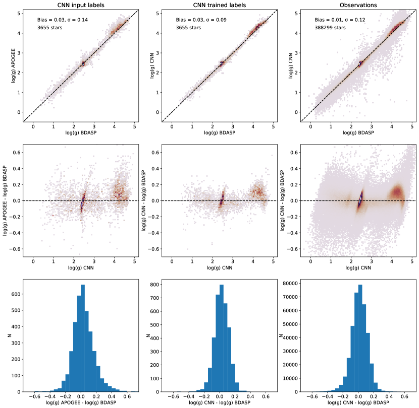
Figure 15: Left: Comparisons of the $\text{log}(\textit{g})$ values used as input labels of our CNN (APOGEE DR16 $\text{log}(\textit{g})$) with respect to $\text{log}(\textit{g})$ values of Steinmetz et al. (2020a). We also show a residual plot and an histogram of the difference. Mean difference and scatter are indicated in the top-left corner. Middle: Comparison of $\text{log}(\textit{g})$ values trained by our CNN with respect to $\text{log}(\textit{g})$ values of Steinmetz et al. (2020a). Right: Comparison of the $\text{log}(\textit{g})$ values derived by our CNN for $388\,299$ stars of our observed sample with respect to the $\text{log}(\textit{g})$ values of Steinmetz et al. (2020a).

6.3 Validation of effective temperatures with IRFM temperatures

A data product of the sixth data release of RAVE is the effective temperature derived via to the Infrared Flux Method (IRFM, Casagrande et al. 2006, 2010, see Steinmetz et al. 2020a for more details). In this section, we compare our effective temperatures to those provided by RAVE DR6. We compared the $\textit{T}_{\text{eff}}$ used in the training sample (APOGEE DR16 $\textit{T}_{\text{eff}}$), those learned by the network, and those derived for the observed sample (for S/N¿20).

The results are presented in Figure 16. We first see that there is a shift between the effective temperatures used as labels in our study and those of Steinmetz et al. (2020a) for hot stars ($\textit{T}_{\text{eff}}>5\,200\,$K) which are offset by -250 K (constant with temperature, with 260 K scatter). Those stars are mainly dwarfs. On the other hand, the cool stars of the training sample ($\textit{T}_{\text{eff}}<5\,200\,$K, mostly giants) show a tight and unbiased one-to-one relation with respect to the IRFM temperatures (mean difference of -20 K and dispersion of 90 K). Overall, the dispersion is about 220 K for the 3651 stars of the training sample.

We note that stars with $\textit{T}_{\text{eff}}>5\,200\,$K tend to be cooler by 250 K with respect to the IRFM $\textit{T}_{\text{eff}}$. The $\text{log}(\textit{g})$ of such stars will be then systematically higher. This could serve as an explanation for the higher $\text{log}(\textit{g})$ measured by our CNN with respect to BDASP $\text{log}(\textit{g})$ (see previous section, Figure 15). Once the CNN is trained, the effective temperatures still show the same behaviour with respect to the IRFM $\textit{T}_{\text{eff}}$.

Finally, we can see that the measured $\textit{T}_{\text{eff}}$ in $371\,166$ stars of the observed sample match in the same way the RAVE IRFM $\textit{T}_{\text{eff}}$, with a larger scatter than the training sample mainly due to the presence of stars with lower S/N. Overall, the effective temperatures used in the training sample (from APOGEE DR16), those trained, and those predicted agree rather well with the $\textit{T}_{\text{eff}}$ IRFM from Steinmetz et al. (2020a). Finally, we note that this comparison only provides an assessment of the biases and scatter with respect to APOGEE DR16.

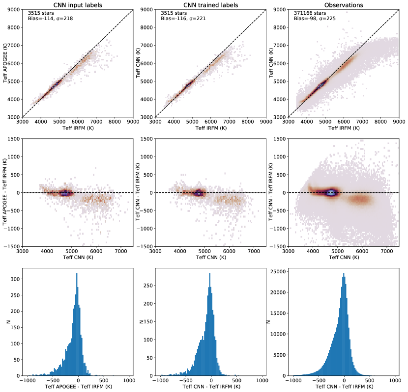
Figure 16: Left: Comparisons of the input label $\textit{T}_{\text{eff}}$ for our CNN (APOGEE DR16 labels) with the IRFM temperatures of Steinmetz et al. (2020a). Mean difference and scatter are indicated in the top-left corner. We also show a residual plot and an histogram of the difference. Middle: Comparison of the labels $\textit{T}_{\text{eff}}$ trained by the CNN with the IRFM temperatures of Steinmetz et al. (2020a). Right: Comparison of the $\textit{T}_{\text{eff}}$ values derived for our whole observed data-set (for S/N¿20) with the IRFM temperatures of Steinmetz et al. (2020a).

6.4 Validation with repeat observations

Another way to show the reliability of our atmospheric parameters and chemical abundances is to investigate stars with repeated observations. We follow the same procedure as in Steinmetz et al. (2020b, a). Briefly, for a given star with several observations, we computed the differences in atmospheric parameters and chemical abundances. For all stars with multiple repeats, we analyzed the distribution of those differences. We approximated the distribution function by a combination of two Gaussians using a least-squares fit. The results are presented in Figure 17, for all repeats ($80\,342$ stars, $S/N>20$). Firstly, we can see that the distributions are roughly similar in shape for $\textit{T}_{\text{eff}}$, $\text{log}(\textit{g})$, $[\text{M}/\text{H}]$, and $[\text{Fe}/\text{H}]$. On the other hand, the chemical abundances of $[\alpha/\text{M}]$, $[\text{Mg}/\text{Fe}]$, $[\text{Si}/\text{Fe}]$, $[\text{Al}/\text{Fe}]$, and $[\text{Ni}/\text{Fe}]$ present asymmetric tails. The typical dispersion of the distribution for the effective temperature is about $\sim 50\,$K, while for the surface gravity, the dispersion is below 0.05 dex. The dispersion increases to $80\,$K for $\textit{T}_{\text{eff}}$ and 0.14 dex for $\text{log}(\textit{g})$ if we do not use photometry to introduce additional information. For $[\text{M}/\text{H}]$ and $[\text{Fe}/\text{H}]$, the typical dispersion over all repeats is of the order of 0.05 dex. Finally, for $[\alpha/\text{M}]$, $[\text{Mg}/\text{Fe}]$, $[\text{Si}/\text{Fe}]$, $[\text{Al}/\text{Fe}]$, and $[\text{Ni}/\text{Fe}]$, a dispersion of 0.02-0.03 dex is measured over all repeats. These results imply that the CNN is precise (low dispersion within repeats) and accurate (overall difference distributions centered on zero) in determining atmospheric parameters and chemical abundances of RAVE spectra. We note that such dispersion within repeats in consistent with the typical uncertainties reported in Sect. 5 for both atmospheric parameters and chemical abundances.

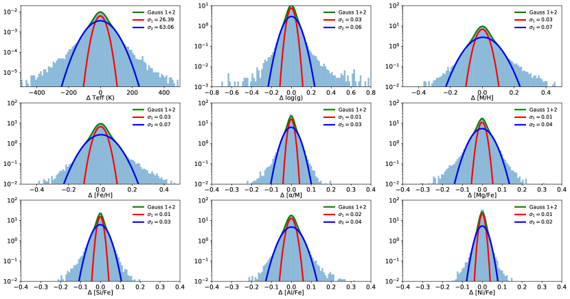
Figure 17: Differences in atmospheric parameters and chemical abundances for $80\,342$ stars based on several observations and $S/N>20$.

6.5 Comparison with RAVE DR6 $[\alpha/\text{M}]$ ratios

The RAVE spectra cover the near-infrared CaII triplet, which is a key spectral feature in the process of placing constraints on the overall $\alpha$ enrichment of stars. In this section, we compare the $[\alpha/\text{M}]$ derived in the present study by our CNN to the $[\alpha/\text{Fe}]$ derived in Steinmetz et al. (2020a) by a more classical approach (synthetic spectra grid + optimisation method). Both quantities were derived using the same observed spectra.

In Figure 18, we present an abundance pattern comparison between the present study ($[\alpha/\text{M}]$ vs. $[\text{M}/\text{H}]$) and RAVE DR6 ($[\alpha/\text{Fe}]$ vs. $[\text{Fe}/\text{H}]$), for $69\,659$ dwarfs and giants ($S/N>20$). We adopt the same quality criteria presented in Steinmetz et al. (2020a) to select the best RAVE DR6 $[\alpha/\text{Fe}]$ ratios.

We first show a typical Kiel diagram for each sample (CNN top-left, RAVE DR6 top-right). Using our CNN approach with combined spectroscopy, photometry and astrometry, we are able to tackle the degeneracy caused by RAVE’s narrow wavelength range, especially in the very cool regime.

The abundances derived by RAVE DR6 show a larger scatter at a given metallicity. In the metal-poor regime, the CNN results show a tight $[\alpha/\text{M}]$ sequence. Overall, both studies show the same main chemical features, for both giants and dwarfs. They also cover the same metallicity range. We note that in the metallicity range of $-1<[\text{M}/\text{H}]<+0\,$dex, the CNN $[\text{M}/\text{H}]$ present a shift of +0.14 dex with respect to RAVE DR6 $[\text{Fe}/\text{H}]$, while for both metal-poor and metal-rich tails, the bias is basically null. The differences in trends and zero-points originate from a different calibration between the two studies, one based on APOGEE data, while the RAVE DR6 is based on synthetic spectra grid.

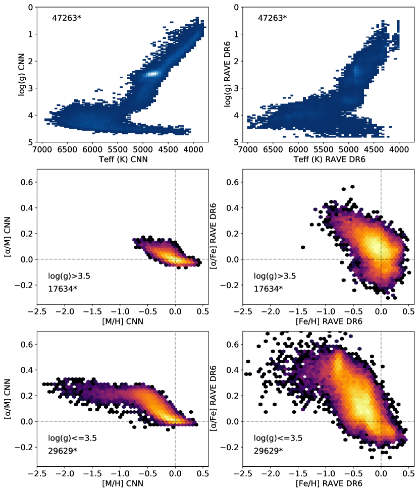
Figure 18: Top: $\textit{T}_{\text{eff}}$ vs. $\text{log}(\textit{g})$ for 69959 stars, derived with our CNN (left) and derived by RAVE DR6 (right). Middle: Abundance pattern for $30\,988$ dwarfs, derived by our CNN (left) and RAVE DR6 (right). Bottom: Same plots for $38\,671$ giants.

6.6 Exotic star detection capabilities

Neural networks are particularly efficient with regard to classifying objects. In addition, peculiar stars are expected to be detected by such a machine-learning pipeline; by peculiar, we mean that the CNN is able to parameterise stars in regions where the training sample parameter space is poorly covered. We illustrate this point by the example of the known yellow supergiant (spectral type F3I, Houk 1978, Gaia_sourceid=’5983723702088571392’), which has been observed six times by the RAVE survey. The normalised RAVE DR6 spectra are presented in Figure 19. This star has been characterised as ’normal’ by RAVE DR6. Its Gaia DR2 parallax error is 10%. The mean atmospheric parameters and errors derived by our CNN from the six repeats are the following: $\textit{T}_{\text{eff}}=5423\pm 355\,$K, $\text{log}(\textit{g})=1.02\pm 0.53$, $[\text{M}/\text{H}]=-0.36\pm 0.20\,$dex. The average RAVE DR6 parameters derived with the BDASP pipeline (using Gaia DR2 and isochrone fitting) are the following: $\textit{T}_{\text{eff}}=5047\pm 213\,$K, $\text{log}(\textit{g})=1.39\pm 0.08$, $[\text{M}/\text{H}]=+0.28\pm 0.15\,$dex. In spite of the differences in the approach, the CNN and BDASP methods tend to put this star in the same region of the Kiel diagram, within 1-$\sigma$ errors. The overall metallicity shows the largest scatter, with CNN and BDASP consistent within 2-$\sigma$.

On the other hand, the RAVE DR6 parameters by the MADERA pipeline (pure spectroscopy) are the following: $\textit{T}_{\text{eff}}=5986\pm 95\,$K, $\text{log}(\textit{g})=3.63\pm 0.15$, $[\text{M}/\text{H}]=+0.51\pm 0.09\,$dex. Those parameters are consistent to those derived by our CNN, only using spectroscopic data (no photometry or parallaxes), within 2-$\sigma$ in $\textit{T}_{\text{eff}}$ and 1-$\sigma$ in $\text{log}(\textit{g})$ and $[\text{M}/\text{H}]$: $\textit{T}_{\text{eff}}=6401\pm 150\,$K, $\text{log}(\textit{g})=3.90\pm 0.20$, $[\text{M}/\text{H}]=+0.50\pm 0.11\,$dex.

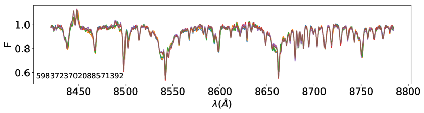
Figure 19: Normalised RAVE DR6 spectra of the target Gaia ’5983723702088571392’. The six spectra are plotted in different colours.

7 Including versus excluding photometry

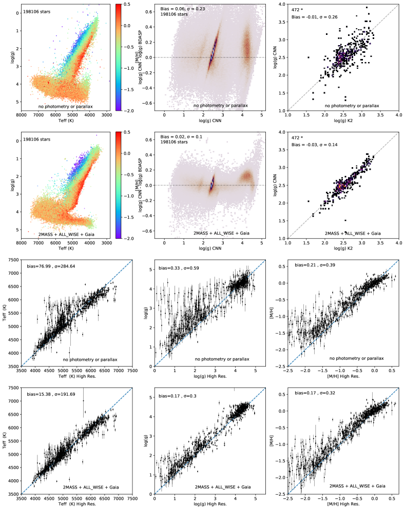
Figure 20: Systematic comparisons of parameters from our CNN with or without photometry (2MASS+ALL_WISE+GaiaDR2) and astrometry (Gaia DR2). Top-left: The Kiel diagrams are colour-codded in $[\text{M}/\text{H}]$ for $198\,106$ stars (’n&o’ classification) with $S/N>40$ and parallax errors lower than $20\%$; Top middle: Comparison of $\text{log}(\textit{g})$ with respect to RAVE DR6 $\text{log}(\textit{g})$ for the same stars; Top-right: Comparison of CNN $\text{log}(\textit{g})$ values with respect to K2 $\text{log}(\textit{g})$ values; Bottom: Comparisons of CNN $\textit{T}_{\text{eff}}$, $\text{log}(\textit{g})$, and $[\text{M}/\text{H}]$ values with respect to the high-resolution sample (one-to-one relations).

We show here that adding absolute photometric magnitudes during the training phase of the CNN significantly improves the quality of the derived effective temperature and surface gravity, and, to a lesser extent, the overall metallicity. We recall that colours are key indicators of effective temperatures and that colours and absolute magnitudes help to constrain surface gravities.

To do so, we simply re-trained our CNN a hundred times, with the same overall architecture but removing the photometric neurons, meaning that we only use pure spectroscopic data from RAVE. We kept the same training sample. We simultaneously predicted $\textit{T}_{\text{eff}}$, $\text{log}(\textit{g})$, $[\text{M}/\text{H}]$, $[\text{Fe}/\text{H}]$, plus individual abundances for the observed data.

In Figure 20, we present the resulting Kiel diagram of $\textit{T}_{\text{eff}}$ and $\text{log}(\textit{g})$, colour-coded in $[\text{M}/\text{H}]$. We only show data with $S/N>40$, that is, stars with good observational data. Compared to the Kiel diagram derived including absolute magnitudes, the pure spectroscopic results still have all the typical features, like the cool dwarf sequence, the turn-off, or the giant branch. On the other hand, the cool dwarfs sequence suffers from large scatter, while degeneracies appear for very cool giants (large $\text{log}(\textit{g})$ scatter for a given $\textit{T}_{\text{eff}}$). The red giant branch appears as a straight sequence. Finally, the metallicity sequence in the giant branch is not as well-defined as when absolute magnitudes are used. The wavelength range around the CaII triplet is known to suffer from degeneracies when deriving atmospheric parameters (Kordopatis et al. 2011a). We note that including absolute magnitudes helps us to break these degeneracies, without applying any prior or restraining the parameter space of the training sample. The mean error in $\textit{T}_{\text{eff}}$ is increased by $\sim 20\,$K when no absolute magnitudes are used.

We then compare our surface gravities with those from RAVE BDASP $\text{log}(\textit{g})$. When using 2MASS+ALL_WISE+Gaia, we can see that the average difference between both studies is one quarter of the one based purely on spectroscopy, while the dispersion drops from 0.23 to 0.09 dex.

Next, we compare our purely spectroscopic $\text{log}(\textit{g})$ values to those provided by K2. Without photometric input, the scatter is much larger (0.26 dex) with a tiny bias. We note that the purely spectroscopic $\textit{T}_{\text{eff}}$ values show a slightly higher dispersion with respect to those derived including absolute magnitudes during the training phase.

Finally, we compare $\textit{T}_{\text{eff}}$, $\text{log}(\textit{g})$, and $[\text{M}/\text{H}]$ derived from purely spectroscopic data by our CNN to those of the high-resolution sample presented in Appendix C (only stars with $S/N>20$). Without absolute magnitudes, we observed a significantly larger dispersion in $\text{log}(\textit{g})$ (0.58 dex) and bias (+0.26 dex), as compared to the high-resolution sample. This is also the case for the effective temperature, with a slightly larger bias (55 K instead of no bias) and a dispersion larger by 80 K. Finally, the metallicity derived purely by spectroscopic data suffers from a slightly higher bias and dispersion with respect to the literature sample. The main improvement is actually notable for $[\text{M}/\text{H}]$¡-1.5 dex, consistent with previous remarks on the Kiel diagram.

With these comparisons, we demonstrate that purely spectroscopic data can still provide quite satisfying outputs, however, adding photometry as well as astrometric parallaxes provides a major gain with a strong increase in precision and accuracy, mainly for effective temperature and surface gravity. We are able to efficiently break the degeneracies in the $\textit{T}_{\text{eff}}-\text{log}(\textit{g})$ space, caused by limited spectral range of RAVE spectra, particularly in the cool regime.

8 Science verification

8.1 Abundance-kinematical properties of the Milky Way components

Here, we investigate some implications for the chemical and kinematical properties of the Milky Way. We adopted the kinematics from RAVE DR6 (Steinmetz et al. 2020a) and followed the same approach as Gratton et al. (2003) and Boeche et al. (2013a). We first kinematically selected a thin disc component with low eccentricity stars ($e<0.25$) and low maximum altitude ($\text{Z}_{\text{max}}<0.8\,$kpc). We identified a dissipative collapse component, mainly composed of thick disc and halo stars with $e>0.25$, $\text{Z}_{\text{max}}>0.8\,$kpc, and $V_{\phi}>40\,$km s^-1. Finally, we characterised an accretion component, composed of halo and accreted stars ($V_{\phi}<40\,$km s^-1).

In Figure 21, we present the $[\alpha/\text{M}]$ pattern for these three components for giant stars ($\text{log}(\textit{g})<3.5$). The thin disc is mainly confined to $[\text{M}/\text{H}]>-1\,$dex, while the dissipative collapse component shows a large metallicity range, a few metal-rich stars, including halo stars with metallicities higher than $-2\,$dex, and a narrow $[\alpha/\text{M}]$ sequence. The accretion component is only composed of metal-poor stars, in the range $-2.0<[\text{M}/\text{H}]<-0.5$. We note that the mean error on $[\text{M}/\text{H}]$ and $[\alpha/\text{M}]$ increases with decreasing metallicity for the three components. These findings are in good agreement with Boeche et al. (2013a).

We measured the gradients of $V_{\phi}$ vs. $[\text{M}/\text{H}]$ in both the thin disc and dissipative collapse components. The thin disc component shows an anti-correlation ($\nabla=-20$km s^-1/dex), while a strong correlation is visible in the dissipative collapse component ($\nabla=+54$km s^-1/dex). Such gradients are consistent with previous works, like for example Lee et al. (2011) with SEGUE data or Kordopatis et al. (2011b), despite different selection functions. We note, however, that the positive gradient in the dissipative collapse components results from the superposition of mono-$[\alpha/\text{M}]$ sub-populations with negative slopes, as was recently shown using RAVE DR5 data (Wojno et al. 2018; Minchev et al. 2019). These simple science applications show the potential of the CNN abundances.

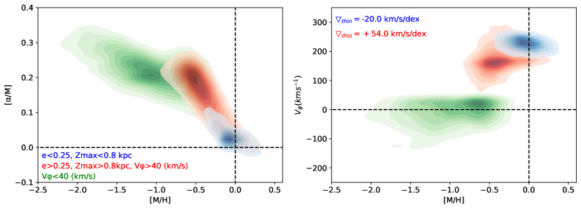
Figure 21: Left: $[\alpha/\text{M}]$ vs. $[\text{M}/\text{H}]$ contour plots of the thin disc component (75 642 stars, blue), the dissipative collapse component (15 433 stars, red), and the accretion component (1 400 stars, green). Right: Galactocentric rotational velocities $V_{\phi}$ as a function of $[\text{M}/\text{H}]$. We only show stars with parallax errors lower than $20\%$, $S/N>40$ and ’n&o’ RAVE classification. We estimated the gradients of $V_{\phi}$ vs. $[\text{Fe}/\text{H}]$ in the thin disc component and in the dissipative collapse component and find good agreement with literature values, depsite our different selection criteria (see for example Kordopatis et al. (2011b) and Lee et al. (2011)).

8.2 Chemical cartography of $[\alpha/\text{M}]$ ratio in the galactic discs

In this section, we investigate the spatial transition between the $[\alpha/\text{M}]$-rich and $[\alpha/\text{M}]$-poor populations of the Milky Way. We once again take advantage of the orbital parameters provided by the sixth data release of RAVE (Steinmetz et al. 2020a). We present, in Figure 22, the behaviour of the $[\alpha/\text{M}]$ ratio as a function of $[\text{Fe}/\text{H}]$ for different bins of mean Galactocentric radii ($R$) and heights above the Galactic plane ($|Z|$). The figure shows hexagonal density maps and contour plots for a total of $185\,569$ giant stars with $S/N>30$, parallax errors lower than $20\%$, and RAVE ’n&o’ classification. We observe that the $[\alpha/\text{M}]$-poor population dominates at low Galactic heights ($|Z|<0.5$kpc), while $[\alpha/\text{M}]-$rich stars are mostly located at larger height above the plane ($|Z|>0.5$kpc). In between, there is a very smooth transition. We note that such observations are also valid for the $[\text{Mg}/\text{Fe}]$ and $[\text{Si}/\text{Fe}]$ ratios, with slightly larger scatter. We find consistent results with the study of Hayden et al. (2015) based on APOGEE DR12. For the same Galactic volume, our results are a good match with the recent study by Queiroz et al. (2020) based on APOGEE DR16. We show that we are able to complement RAVE DR6 and ultimately provide chemical abundance trends for a larger sample of stars with improved precision.

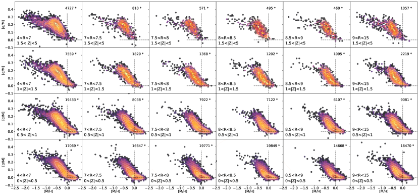
Figure 22: $[\alpha/\text{M}]$ ratio as a function of $[\text{Fe}/\text{H}]$ for several bins of $R$ and $|Z|$. $[\alpha/\text{M}]$ and $[\text{Fe}/\text{H}]$ were derived through our CNN while the $R$ and $|Z|$ come from the DR6 of RAVE (Steinmetz et al. 2020a). Hexagonal bins and contour plots of the data are presented together. In total, we present trends for $185\,569$ stars with $S/N>30$, parallax errors lower than $20\%$, and RAVE ’n&o’ classification.

9 Caveats

The present project relies entirely on the cross-match between a few thousand RAVE and APOGEE targets, which, together with the limitations of the two respective surveys, results in a number of possible caveats.

Firstly, the spectral range of RAVE spectra, $[8\,410-8\,795]$Å, contains plenty of features with which to derive $[\alpha/\text{M}]$ ratios, such as Ca, Ti, Mg, Si, and O spectral lines. The $[\alpha/\text{M}]$ labels adopted here come from the DR16 of APOGEE. This survey uses a different wavelength range (1.51–1.70$\mu$m), nonetheless, its wavelength coverage contains similar elements as RAVE contributing to the $[\alpha/\text{M}]$ mixture, apart from Ne and S. On the other hand, it is known that the most significant contributors of the spectral features are Ca, Ti, Si, O, and Mg. In this context, using the RAVE spectral range to constrain $[\alpha/\text{M}]$ is reasonable.

Secondly, we clearly have a lack of stars at low metallicity ($[\text{M}/\text{H}]\lesssim-1$) in the training sample, which us mainly due to the fact that we have few metal-poor stars in RAVE (Matijevič et al. 2017) and in the cross-match with APOGEE DR16. The mapping of the parameters space for those stars is quite limited. For future studies, it is important to carefully build a training sample with good mapping of the parameters in the metal-poor regime. More and more metal-poor stars are being observed, for example, in the Pristine Survey (Starkenburg et al. 2017; Youakim et al. 2017) and they are key stars for obtaining a more homogeneous mapping of the parameters space.

Finally, out of the approximately $400\,000$ stars of the APOGEE survey DR16, our training sample contains roughly $4\,000$ stars in common with the RAVE survey. It is clear that in the present study the performances of our CNN approach is limited by the small size of the training sample. We have seen that the training and test samples can then suffer from slightly different coverage in the parameter space. The APOGEE and RAVE surveys are characterised by different selection functions. The selection function of the training sample is then characterised by traits common to both surveys. This is a caveat in our study, but the goal for the moment is not to characterise the selection function in full as this will be the object of a future study. Our message here to the community is that we call for everyone to make a special effort to creating unbiased training samples, especially for the next generation of spectroscopic surveys, such as 4MOST, GAIA and WEAVE.

10 Database and public code

Here, we present our catalogue of atmospheric parameters ($\textit{T}_{\text{eff}}$, $\text{log}(\textit{g})$ and $[\text{M}/\text{H}]$), along with chemical abundances ($[\text{Fe}/\text{H}]$, $[\alpha/\text{M}]$, $[\text{Si}/\text{Fe}]$, $[\text{Mg}/\text{Fe}]$, $[\text{Al}/\text{Fe}]$, and $[\text{Ni}/\text{Fe}]$) for $420\,165$ stars (summarised in Table 1). The data table is available at: doi://10.17876/rave/dr.6/19.

Col	Format	Units	Label	Explanations
1	char	-	rave_obs_id	RAVE Obs ID
2	char	-	sourceid	Gaia Source ID
3	float	K	teff	Effective temperature
4	float	K	eteff	Error of $\textit{T}_{\text{eff}}$
5	int	-	flag_teff	Boundary flag for $\textit{T}_{\text{eff}}$
6	float	cm s-2	logg	Surface gravity
7	float	cm s-2	elogg	Error on $\text{log}(\textit{g})$
8	int	-	flag_logg	Boundary flag for $\text{log}(\textit{g})$
9	float	dex	mh	Overall metallicity
10	float	dex	emh	Error on $[\text{M}/\text{H}]$
11	int	-	flag_mh	Boundary flag for $[\text{M}/\text{H}]$
12	float	dex	feh	$[\text{Fe}/\text{H}]$ ratio
13	float	dex	efeh	Error on $[\text{Fe}/\text{H}]$
14	int	-	flag_feh	Boundary flag for $[\text{Fe}/\text{H}]$
15	float	dex	alpham	$[\alpha/\text{M}]$ ratio
16	float	dex	ealpham	Error on $[\alpha/\text{M}]$
17	int	-	flag_alpham	Boundary flag for $[\alpha/\text{M}]$
18	float	dex	sife	$[\text{Si}/\text{Fe}]$ ratio
19	float	dex	esife	Error on $[\text{Si}/\text{Fe}]$
20	int	-	flag_sife	Boundary flag for $[\text{Si}/\text{Fe}]$
21	float	dex	mgfe	$[\text{Mg}/\text{Fe}]$ ratio
22	float	dex	emgfe	Error on $[\text{Mg}/\text{Fe}]$
23	int	-	flag_mgfe	Boundary flag for $[\text{Mg}/\text{Fe}]$
24	float	dex	alfe	$[\text{Al}/\text{Fe}]$ ratio
25	float	dex	ealfe	Error on $[\text{Al}/\text{Fe}]$
26	int	-	flag_alfe	Boundary flag for $[\text{Al}/\text{Fe}]$
27	float	dex	nife	$[\text{Ni}/\text{Fe}]$ ratio
28	float	dex	enife	Error on $[\text{Ni}/\text{Fe}]$
29	int	-	flag_nife	Boundary flag for $[\text{Ni}/\text{Fe}]$
20	float	/pix	snr	Signal-to-noise ratio

Table 1: Atmospheric parameters, chemical abundances, and boundary flags of the publicly available online catalogue for $420\,165$ stars.

The CNN architecture, stellar labels, stellar photometry and spectra used in this paper are accessible via ”https://github.com/gguiglion/CNN_Guiglion_et_al_2020”. The CNN can be easily applied to any current spectroscopic archive or survey to derive atmospheric parameters, chemical abundances, and also other extra parameters such as rotational velocity.

11 Conclusion

Here, we list here the main results of our study.

Based on APOGEE DR16, we built a training sample composed of $3\,904$ stars in common with RAVE DR6. These stars have high quality atmospheric parameters and chemical abundances for $[\text{Fe}/\text{H}]$, $[\alpha/\text{M}]$, $[\text{Si}/\text{Fe}]$, $[\text{Mg}/\text{Fe}]$, $[\text{Al}/\text{Fe}]$, and $[\text{Ni}/\text{Fe}]$, which we use as labels. We built a CNN using the Keras libraries in Python to train the labels defined above. Using these trained labels, we predicted atmospheric parameters and chemical abundances for $420\,165$ RAVE spectra, with our results available online. Our catalogue covers a larger range of S/N than RAVE DR6, and extends the scientific output of the RAVE spectra.

Next, we used ALL_WISE W1&2, 2MASS $JHK_{s}$ and Gaia DR2 $G$, $G_{BP}$, and $G_{RP}$ apparent magnitudes, and extinction estimates to derive absolute magnitudes. We included them in the training process and showed that CNNs are efficient in combining spectroscopic and photometric data. We gain a dramatic advantage in precision and accuracy, especially in $\textit{T}_{\text{eff}}$ and $\text{log}(\textit{g})$, where spectral features are overly degenerate (cool main sequence stars, metal-poor giants, and very cool giants). We demonstrated that such a comprehensive combination of spectra, photometry, and parallaxes allows us to efficiently break degeneracies when the spectral range is too narrow to provide strong constraints on surface gravity.

In performing a hundred training phases, we derived errors of the atmospheric parameters, which typically amount to 60 K in $\textit{T}_{\text{eff}}$, 0.06 in $\text{log}(\textit{g})$, and 0.02-0.04 dex for individual chemical abundances. Such high precision is realistic because the network is able to learn the low- and high-$\alpha$ sequences in the Milky Way disc. We show that for stars with several observations, the network is able to provide precise atmospheric parameters and abundances among the repeats that typically precise to 50 K in $\textit{T}_{\text{eff}}$ and 0.03-0.05 dex in abundances.

We show that the surface gravities match nicely with more than 430 asteroseismic gravities from the K2 space mission within 0.14 dex dispersion and no bias. We compared our effective temperature and surface gravities with respect to both the IRFM $\textit{T}_{\text{eff}}$ and $\text{log}(\textit{g})$ from the DR6 of RAVE and we were able to characterise the systematics between the two studies.

It is important to note that different trends and zero-point offsets between this work and external studies primarily reflect the different calibrations applied to these surveys. A systematic comparison between different surveys is therefore crucial. Furthermore, the CNN architecture and weights will be publicly available.

Despite quite a low number statistics in the training sample with respect to the number of free parameters to fit, we show that such an approach can provide solid scientific output. Of course, the performance would improve a lot if the size of the training sample was three to four times larger, but this pilot study is limited by the current overlap with APOGEE DR16. This study allowed us to highlight possible bias and systematics induced by using a limited-size training sample with a CNN machine-learning method. For the next generation of surveys, the community will have to put strong efforts into producing large and un-biased training samples.

Our study shows that CNNs are particularly efficient in transferring knowledge from one survey at high resolution, such as APOGEE, to another at lower resolution, such as RAVE. This study gives good insights for ongoing and future spectroscopic surveys, such as Gaia-RVS and 4MOST. The Gaia-RVS spectra are expected to be very similar to those of RAVE (R$\sim$11400) and we show that adding photometry breaks spectral degeneracies; photometry will be available for all RVS targets. Efficient training of Gaia-RVS data based on higher-resolution surveys could deliver atmospheric parameters and abundances for a larger number of RVS stars, as it is the case for RAVE in the present paper. The low-resolution 4MOST spectra will cover a much larger spectral range ($4\,000-9\,000$ Å) at a slightly lower resolution than Gaia for the 4MIDABLE-LR low-resolution survey (Chiappini et al. 2019), and Gaia photometry will also be available for all targets. Additional constraints could then be put on the derivation of $\textit{T}_{\text{eff}}$ and $\text{log}(\textit{g})$ by coupling spectroscopy, photometry, and astrometry. Such surveys will deliver millions of spectra that can be analysed in only a few minutes on a single graphics processing unit once the labels are trained.

Appendix A Effect of parallax errors on CNN performance

In the present study, 94% of the RAVE DR6 targets have good Gaia DR2 parallaxes, with an error better than $20\%$. Deriving absolute magnitudes from such parallaxes and apparent magnitudes is then safe in the context of the present paper. This high success rate is, however, an immediate consequence of the relatively bright magnitude limit of $I<13$ for RAVE, with the majority of the stars even having $I<12$. The overall Gaia RVS survey will, however, probe considerably fainter objects. The low-resolution surveys like Gaia RVS or 4MIDABLE-LR of 4MOST (Chiappini et al. 2019) will probe a much larger volume than RAVE. There is then a risk that many targets suffer from large parallax errors. Here, we discuss the impact of such large parallax errors on the determination of atmospheric parameters and abundances.

In Figure 23, we present CNN results for $3\,502$ stars of the observed sample with parallax errors, $e_{p}>20\%$, and $S/N>50$ per pixel. Despite the large parallax errors, we can recover a proper giant branch with a clear metallicity sequence. Most of the stars with $e_{p}>40\%$ are actually located in the upper part of either the main sequence or the cool giant branch. Such stars should be thus used with caution. For all stars with $e_{p}>20\%$, the $[\alpha/\text{M}]$ versus $[\text{M}/\text{H}]$ abundance patterns do not show systematics, meaning that chemical abundances are less sensitive to less precise parallaxes (absolute magnitudes constraining mainly $\textit{T}_{\text{eff}}$ and $\text{log}(\textit{g})$).

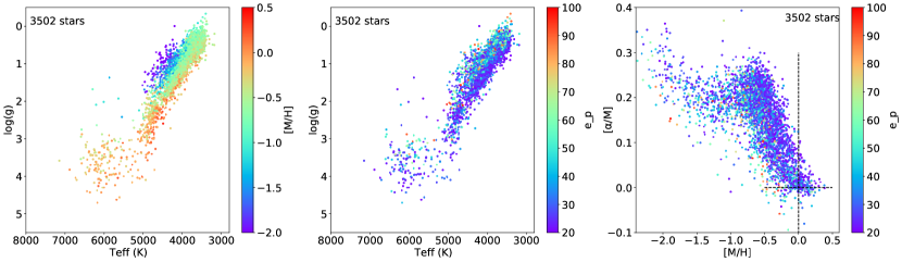
Figure 23: Kiel diagram of $3\,502$ stars of the observed sample, with $e_{p}>20\%$, colour-coded by $[\text{M}/\text{H}]$ (top panel) and $e_{p}$ (middle panel). Only stars with $S/N>50$ per pixel are plotted. The same stars are presented in the bottom panels in the $[\alpha/\text{M}]$ versus $[\text{M}/\text{H}]$ plane, colour-coded by parallax errors.

To check if the CNN could learn from lower quality data, we added in our training sample $\sim 150$ more stars with parallax errors higher than 20%. Adding such stars did not improve the training phase or the atmospheric parameters of the observed sample stars with parallax errors larger than 20%.

Appendix B Validation of atmospheric parameters with stellar clusters

Here we compare the CNN results with 41 stars from four clusters used in RAVE DR6 for calibration purposes: 47Tuc (Carretta et al. 2009), Pleiades (Funayama et al. 2009), Blanco1 (Ford et al. 2005), IC4651 (Pasquini et al. 2004), and Omega Centauri (Johnson & Pilachowski 2010). The results are presented in Figure 24.

The giants tend to match pretty well between our study and the literature, with slight variations from cluster to cluster. The Pleiades show no discernible offset in $\text{log}(\textit{g})$ and $[\text{Fe}/\text{H}],$ while a large mean difference is measured for $\textit{T}_{\text{eff}}$ (-353 K). We have both giant and dwarf stars in common with IC4651, and they tend to show a good match with our study. The dispersion in $[\text{Fe}/\text{H}]$ drops to 0.03 when only considering stars with $S/N>40$. We only have one star in common with Blanco 1, but we find good agreement between the literature and our study. Finally, the cluster 47Tuc presents an offset of +0.13 dex in $[\text{Fe}/\text{H}]$ with respect to the literature, while the dispersion is about 0.1 dex. We note that we have a total of 13 stars from 47Tuc and the Pleiades in our training sample. We have 12 giants in common with the metal-poor globular cluster Omega Centauri. The $[\text{Fe}/\text{H}]$ values of our CNN do not show any bias with respect to the literature, and the dispersion is about 0.1 dex. The Omega Centauri stars span lower $\text{log}(\textit{g})$ values that 47Tuc, mainly $\text{log}(\textit{g})<1$. We show that the CNN is able to provide reliable parameterisation of metal-poor super-giant stars.

The systematics observed in the three parameters come directly from systematics in the APOGEE DR16 labels. Overall, the typical dispersion $\sigma$ in $\textit{T}_{\text{eff}}$ and $[\text{Fe}/\text{H}]$ tends to decrease when selecting stars with $S/N>40$, but stays constant for $\text{log}(\textit{g})$.

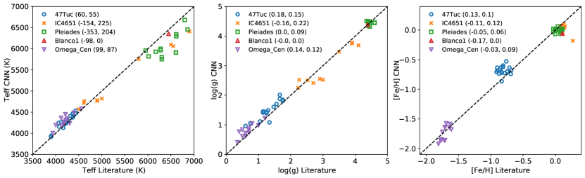
Figure 24: Comparison of $\textit{T}_{\text{eff}}$, $\text{log}(\textit{g})$, and $[\text{Fe}/\text{H}]$ between the present study and compilation of five stellar clusters with common stars with RAVE: 47Tuc ($\circ$), IC4651 ($\times$), Pleiades ($\square$), Blanco1 ($\triangle$), and Omega Centauri ($\triangledown$). The mean difference and dispersion are indicated together with the cluster name.

Appendix C Validation of atmospheric parameters and chemical abundances with the HR sample

Here, compare our atmospheric parameters and chemical abundances with those from high-resolution (HR) studies in the literature. We took a high resolution sample compiled and used for validation purposes in RAVE DR6 (Steinmetz et al. 2020a). It includes more than 1700 stars, taken from several studies, among them with available chemical abundances Reddy et al. (2003); Valenti & Fischer (2005); Soubiran & Girard (2005); Reddy et al. (2006); Ruchti et al. (2011); Adibekyan et al. (2012); Bensby et al. (2014) and Gaia-ESO Survey DR5.

We present a Kiel diagram and abundance patterns for stars of the high-resolution sample and from the present study in Figure 25. We only selected stars with $S/N>20$. Basically, the main and giant sequences match pretty well. The $[\alpha/\text{M}]$, $[\text{Si}/\text{Fe}]$ patterns tend to match for $[\text{Fe}/\text{H}]>-0.5\,$dex, while at lower metallicity the CNN abundances tend to be systematically lower. This comes from the fact that $[\alpha/\text{M}]$ and $[\text{Si}/\text{Fe}]$ do not reach values higher than +0.30 dex in APOGEE DR16. On the other hand, $[\text{Mg}/\text{Fe}]$ matches rather well between our CNN results and the literature. The $[\text{Al}/\text{Fe}]$ ratios are reasonably consistent around solar $[\text{Fe}/\text{H}]$, but the scatter increases for the metal-poor regime. Finally, $[\text{Ni}/\text{Fe}]$ is rather flat in both samples, as expected for an Fe-peak element.

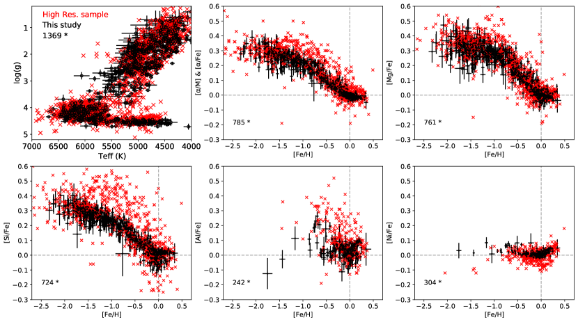
Figure 25: Kiel diagram and chemical abundances patterns for stars in common between our study (black circles) and the literature (red crosses).

In Figure 26, we present the 1-to-1 relations between the high-resolution sample and the present study. This illustrates the differences in the trends and zero-points very well. The typical dispersion is about 200 K in $\textit{T}_{\text{eff}}$ (no bias), while it is around 0.3 for $\text{log}(\textit{g})$ (bias of 0.13 dex) and $[\text{Fe}/\text{H}]$ ($\sim 0.3$ bias). We observe an increase of the scatter with decreasing $[\text{Fe}/\text{H}]$. We note that the overall scatter in $[\text{Fe}/\text{H}]$ drops to 0.2 dex if we only select stars with $S/N>50$. All other abundances show quite a small dispersion, roughly 0.1 dex. In fact, shifts in the trends or in the zero-points reflect more a systematic difference of the calibration between the APOGEE DR16 surveys and the test sample, rather than an incorrect estimation of parameters or abundances. Such differences are to be expected considering the differences in instrument specifications, resolution, wavelength range, and wavelength coverage.

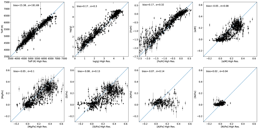
Figure 26: Atmospheric parameters and chemical abundances derived by our CNN, as a function of values from the literature. Mean bias and dispersion are indicated in the top left corner of each panel.

Appendix D Chemical abundance patterns of $[\text{Mg}/\text{Fe}]$, $[\text{Si}/\text{Fe}]$, $[\text{Al}/\text{Fe}]$ and $[\text{Ni}/\text{Fe}]$

In this section, we present chemical abundance patterns of $[\text{Mg}/\text{Fe}]$, $[\text{Si}/\text{Fe}]$, $[\text{Al}/\text{Fe}]$, and $[\text{Ni}/\text{Fe}]$ as a function of $[\text{Fe}/\text{H}]$ in the training and observed samples (S/N¿30 and ”n” stars). Figure 27 and Figure 28 present $[\text{Mg}/\text{Fe}]$ and $[\text{Si}/\text{Fe}]$ abundances patterns for $301\,076$ stars. The trends of both elements look pretty similar to the trends of $[\alpha/\text{M}]$ presented in Figure 12, Si and Mg being $\alpha$-elements. In Figure 29, we present the chemical abundance patterns of $[\text{Al}/\text{Fe}]$ of the same $301\,076$ stars. For $[\text{Fe}/\text{H}]>-1\,$dex, $[\text{Al}/\text{Fe}]$ behaves like an $\alpha-$element (consistent with previous findings in the literature, see for example Smiljanic et al. 2016). For $[\text{Fe}/\text{H}]<-1$, we can see that the $[\text{Al}/\text{Fe}]$ ratio drops to solar – and even down to negative ratios. It is mainly driven by the very few stars we have in the training sample exhibiting low-$[\text{Al}/\text{Fe}]$ ratios. We ought to be particularly careful when using such $[\text{Al}/\text{Fe}]$ abundances. In Figure 30, we present $[\text{Ni}/\text{Fe}]$ ratios for $301\,076$ stars. This ratio is rather flat with $[\text{Fe}/\text{H}]$, as is expected for such an Fe-peak element.

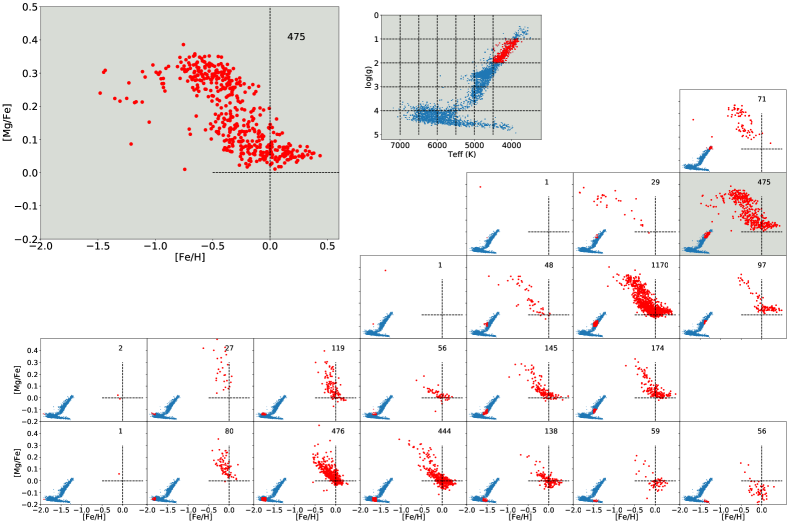
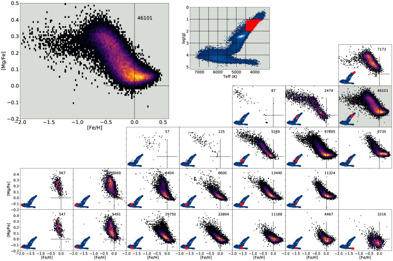
Figure 27: Top: $[\text{Mg}/\text{Fe}]$ vs. $[\text{Fe}/\text{H}]$ for the training sample. Bottom: $[\text{Mg}/\text{Fe}]$ vs. $[\text{Fe}/\text{H}]$ for $301\,076$ stars of the observed sample with S/N¿30, RAVE DR6 ’n&o’ classification, and parallax errors lower than $20\%$. For each panel, we overplotted a $\textit{T}_{\text{eff}}-\text{log}(\textit{g})$ diagram with the location of the plotted stars marked in red.

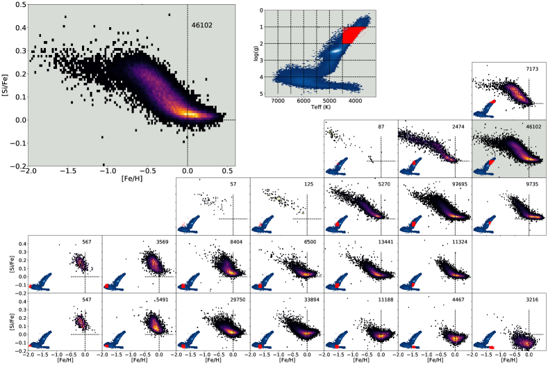
Figure 28: Top: $[\text{Si}/\text{Fe}]$ vs. $[\text{Fe}/\text{H}]$ for the training sample. Bottom: $[\text{Si}/\text{Fe}]$ vs. $[\text{Fe}/\text{H}]$ for $301\,076$ stars of the observed sample with S/N¿30, RAVE DR6 ’n&o’ classification, and parallax errors lower than $20\%$. For each panel, we overplotted a $\textit{T}_{\text{eff}}-\text{log}(\textit{g})$ diagram with the location of the plotted stars marked in red.

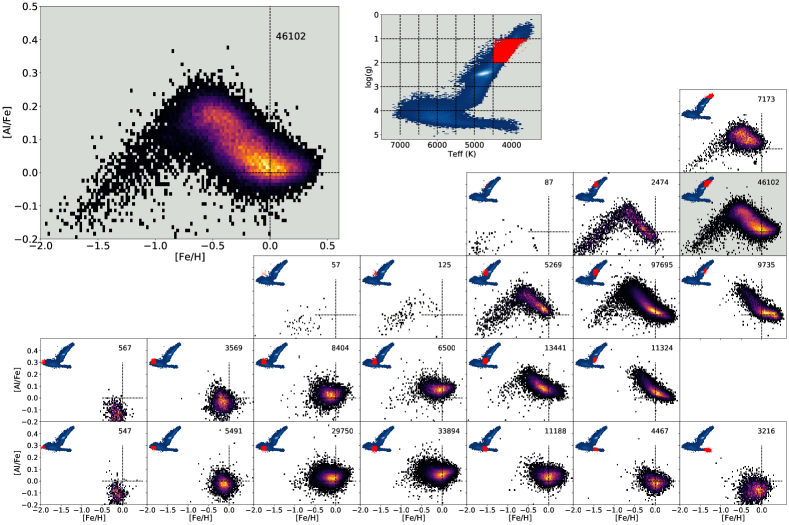
Figure 29: Top: $[\text{Al}/\text{Fe}]$ vs. $[\text{Fe}/\text{H}]$ for the training sample. Bottom: $[\text{Al}/\text{Fe}]$ vs. $[\text{Fe}/\text{H}]$ for $301\,076$ stars of the observed sample with S/N¿30, RAVE DR6 ’n&o’ classification, and parallax errors lower than $20\%$. For each panel, we overplotted a $\textit{T}_{\text{eff}}-\text{log}(\textit{g})$ diagram with the location of the plotted stars marked in red.

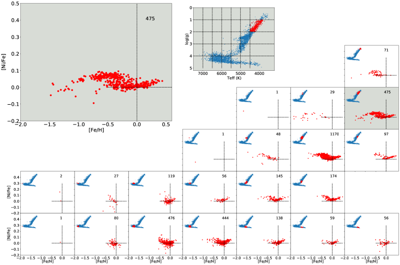
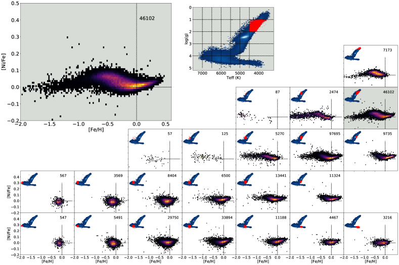
Figure 30: Top: $[\text{Ni}/\text{Fe}]$ vs. $[\text{Fe}/\text{H}]$ for the training sample. Bottom: $[\text{Ni}/\text{Fe}]$ vs. $[\text{Fe}/\text{H}]$ for $301\,076$ stars of the observed sample with S/N¿30, RAVE DR6 ’n&o’ classification, and parallax errors lower than $20\%$. For each panel, we overplotted a $\textit{T}_{\text{eff}}-\text{log}(\textit{g})$ diagram with the location of the plotted stars marked in red.