Observational features of exoplanetary synchrotron radio bursts

Abstract

Magnetic fields of exoplanets are important in shielding the planets from cosmic rays and interplanetary plasma. Due to the interaction with the electrons from their host stars, the exoplanetary magnetospheres are predicted to have both cyclotron and synchrotron radio emissions, of which neither has been definitely identified in observations yet. As the coherent cyclotron emission has been extensively studied in literatures, here we focus on the planetary synchrotron radiation with bursty behaviors (i.e., radio flares) caused by the outbreaks of energetic electron ejections from the host star. Two key parameters of the bursty synchrotron emissions, namely the flux density and burst rate, and two key features namely the burst light curve and frequency shift, are predicted for star - hot Jupiter systems. The planetary orbital phase - burst rate relation is also considered as the signature of star-planet interactions (SPI). As examples, previous X-ray and radio observations of two well studied candidate systems, HD 189733 and V830 $\tau$, are adopted to predict their specific burst rates and fluxes of bursty synchrotron emissions for further observational confirmations. The detectability of such emissions by current and upcoming radio telescopes shows that we are at the dawn of discoveries.

1 Introduction

As the key signal from exoplanetary magnetospheres, there have been efforts in detecting the radio emission from exoplanets since, and even before the discovery of the first exoplanet (Yantis et al., 1977; Bastian et al., 2000; Sirothia et al., 2014; Lynch et al., 2018; Route, 2019). Although radio detections are achieved for a few exoplanetary systems, no definite conclusion has been made about whether the radiations are from the planets, their host stars, or even other radio sources close to the targets (Sirothia et al., 2014; Bower et al., 2016). The difficulty of detection and further confirmation of the exoplanetary radio emissions lies on three factors to be quantified: (I) the emission frequency and corresponding radio flux density, (II) the rate of bursty emissions bearing different energies, and (III) the light curve and possible temporal - frequency shift features of the signal.

Because of the expected high radio flux, efforts in the early champion focus on the detection of exoplanetary coherent cyclotron emissions (also mentioned as electron cyclotron masers (ECM), cf. Wu & Lee, 1979; Dulk, 1985). However, the upper frequency limit of the ECM is only $\sim 40$ MHz for Jupiter and even lower for exoplanets with magnetic fields weaker than that of Jupiter. Observations using the ground based low frequency ($<$ 10 MHz) radio telescopes experience the ionosphere absorption, making the detection of exoplanets very hard. Efforts on this low frequency branch will eventually rely on the future Lunar low frequency radio telescope array. The upcoming SKA, with significant increase of sensitivity, is also expected to detect exoplanetary ECM above a few 10 MHz (Zarka et al., 2015; Pope et al., 2019). On the other hand, there are special systems from which higher frequency ECM is expected. For exoplanets with magnetic fields much stronger than that of Jupiter (Cauley et al., 2019), and white dwarf (WD) - terrestrial planet systems (Willes & Wu, 2005; Vanderburg et al., 2015; Manser et al., 2019), the ECM frequency can reach $\sim 100$ MHz or even higher. Such systems are potentially detectable by LOFAR, GMRT or other state-of-the-art telescopes.

Generally, when we shift to relatively higher radio frequencies of $\sim 100$ MHz to a few tens GHz, the planetary synchrotron emission caused by high speed (relativistic) electrons from the host star dominates the spectra. Considering the well observed X-ray flares from a few exoplanetary systems as the high energy counterparts of their synchrotron emissions (Pillitteri et al., 2010, 2011, 2014; Poppenhaeger et al., 2013; Maggio et al., 2015), the detection of the synchrotron radio emissions is also expected. However, without the amplification mechanism as in cyclotron masers, the synchrotron emission flux is 5 orders of magnitude lower than the ECM emission (Jupiter as an example, cf. Zarka et al., 2015). Extensive observations of Jupiter synchrotron emissions well characterized their flux, bursty behavior and even the particle energy distribution (de Pater, 2004; Kloosterman et al., 2008; Bhardwaj et al., 2009; Lou et al., 2012; Becker et al., 2017). Compared to Jupiter, there are four variations for exoplanetary systems that affect their synchrotron radiation: (1) the distance between the exoplanet and its host star, (2) the magnetic field strength of the exoplanet and the magnetic field structure of the star-planet system, (3) the Lorentz factor of particles from the host star, and (4) the bursty behavior in the host star.

By considering the above four variations, in this paper we calculate the expected synchrotron radio flux density based on the comparisons with Jupiter, and estimate the burst rate according to the results from stellar flares in Section 2; clarify the light curve and frequency shift as the key features of planetary synchrotron radio bursts in Section 3; make a case study for HD 189733 system and V 830 $\tau$ system in Section 4; and conclude and discuss the results in Section 5.

2 The radio synchrotron flux and burst rate

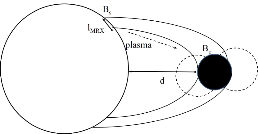
Figure 1: Illustration of the magnetic field structure of a star - planet system close to each other. The left circle is the host star, linked by its magnetic field lines (solid curves) to the planet shown as the black filled circle. Magnetic fields of the planet are shown in dash lines, with its deformation when intercepting the stellar magnetic field not considered. Energetic particles arise from the active regions on the stellar surface and travel to the planet along the magnetic field loops. On the stellar surface, the active region where the magnetic reconnection (MRX) occurs has a typical scale of $l_{\rm MRX}$; and the average orbital radius of the planet is $d$.

For a hot Jupiter enclosed in the magnetosphere of its host star, the magnetic field structure, as well as the energetic particle production and transportation are schematically shown in Fig. 1. Like in binary magnetized stars, radio active star - close planet systems are expected to have the main magnetic field loops originate from the host star and reach the planetary magnetic field (cf. Uchida & Sakurai, 1983; Dulk, 1985; Trigilio et al., 2018; Lanza, 2018). The average magnetic field strength at the stellar surface and planetary surface are noted as $B_{\rm s}$ and $B_{\rm p}$ respectively.

Energetic particles leading to synchrotron radiations are mainly from the coronal mass ejection (CME) in stellar surface through magnetic reconnection (MRX) processes (Zweibel & Yamada, 2009; Ji & Daughton, 2011). In order to estimate the time duration of reconnection, we assume the MRX to occur within a site with the length scale $l_{\rm MRX}$. The charged particles produced from the MRX site then travel along the magnetic field lines and reach the planetary magnetic field, leading to synchrotron emissions at initially the stellar surface and later also the planetary surface. We would also indicate the average orbital radius of the planet $d$, which is important in the following calculations of the particle number at the planet, and the time-lag between the emissions from the star and the planet.

2.1 Exoplanetary quiescent synchrotron radiation power

The frequency of the synchrotron radiation from an electron with Lorentz factor $\gamma$ in magnetic field $B$ is (Rybicki & Lightman, 1979; de Pater, 2004)

$$\nu\simeq 1.3\gamma^{2}B\quad{\rm MHz},$$ (1)

with $B$ in unit of Gauss. Then for the detected electrons with energy $\sim$ 10 MeV in the Jupiter magnetic field of $\sim 4$ G, the synchrotron frequency is up to a few GHz, with the lower end extends to several tens MHz considering the variation of both $\gamma$ and $B$, which is consistent with observations. It is also noted that as a result of both the energy distribution of relativistic electrons and the variation of magnetic field strength, the synchrotron radiation flux from Jupiter between $\sim 100$ MHz to a few GHz varies slightly within 3 to 5 Jy (de Pater, 2004; Kloosterman et al., 2008; Bhardwaj et al., 2009; Girard et al., 2016; Becker et al., 2017), so we roughly consider it as a constant $\sim 4$ Jy.

Based on the synchrotron radiation power of a single electron, the total synchrotron radiation power can be written as

$$P=nP_{\rm e}\propto n\gamma^{2}B^{2},$$ (2)

with $n$ the nominal electron number (without considering specific electron energy distributions). It is readily seen that radiations from an exoplanet and its host star are different in power due to their different magnetic fields. On the other hand, because the corresponding synchrotron radiation cooling time $\tau=8\times 10^{8}B^{-2}\gamma^{-1}\simeq 2\times 10^{6}$ s is much longer than the traveling time of a relativistic electron from the host star to the exoplanet in the case of a typical hot Jupiter ($t=0.1{\rm AU}/c=50$ s), the Lorentz factor of electrons can be considered as the same at the star and the planet. At last we consider the variation of electron nominal numbers in (2) using the total electron numbers instead. In quiescent synchrotron radiations caused by nearly isotropic stellar winds, electrons escape from the entire surface of the host star uniformly rather than from a single MRX site, so the structure in Fig. 1 does not apply. Then the electron number density decreases as $r^{-2}$ as they travel away from the star, and the ratio of the numbers of electrons reach the planet $n_{\rm p}$ and radiate at the star $n_{\rm s}$ can be calculated by simply considering the geometry, i.e.

$$\frac{n_{\rm p}}{n_{\rm s}}=\frac{{R}^{2}}{4d^{2}},$$ (3)

where $R$ is the radius of the planetary magnetosphere. Then the overall ratio between the planetary radiation power and the stellar radiation power is

$$\frac{P_{\rm p}}{P_{\rm s}}=\frac{R^{2}}{4d^{2}}\frac{B_{\rm p}^{2}}{B_{\rm s}^{2}}.$$ (4)

For Jupiter, the estimated power ratio to the solar synchrotron radiation is of the order $0.5\times 10^{-5}$ (where we have adopted the Jupiter magnetic field of 4 G, magnetosphere radius of $\sim$ 20 times the Jupiter radius, and solar magnetic field of 2 G), which is consistent with observations (de Pater, 2004; Grießmeier, 2006). Then for a hot Jupiter with typical orbital radius $\sim 0.1$ AU and magnetic field $\sim 4$ G, if we still assume the magnetic field of its host star to be $\sim 2$ G, the power ratio is $\frac{P_{\rm p}}{P_{\rm s}}\sim 0.8\times 10^{-2}$, i.e., the quiescent radiation power from a hot Jupiter is about $\sim 0.8\%$ of the quiescent radiation power from its host star. Considering that (1) the hot Jupiter magnetic field could be weaker due to possible spin slow-down by tidal lock, (2) the planetary magnetosphere could be smaller in size as it is more compressed being closer to the host star, and (3) the host star magnetic field could be stronger in the K, M or T-Tauri stars which we are interested in, the above power ratio should be usually smaller than $0.8\%$. Of course a larger value of this power ratio is also possible for star - planet systems where the planetary magnetic field is much stronger (cf. Cauley et al., 2019, where the inferred magnetic field should be further confirmed).

2.2 Exoplanetary bursty synchrotron radiation: flux density

Solar bursts have been well observed and classified to several types, among which type IV bursts that originate from the synchrotron emission of energetic electrons ($\sim 10$ MeV) along the corona based magnetic loops are of particular interest for our work. The energetic electrons escape from the star in the CME, which provides an enhanced energetic plasma flux on the planet compared to the quiescent solar wind, and leads to flares in X-ray and radio emissions. The origin of such energetic plasma ejection, although depends on the specific local magnetic field configuration, is generally believed to be the reconnection of magnetic field lines (Isobe et al., 2005; Zweibel & Yamada, 2009; Ji & Daughton, 2011). Then it is natural that for young, late type stars of K and M types including T-Tauri stars, flares are observed to be more common and stronger because of the more active magnetic fields therein (Dulk, 1985; White et al., 1992; Feigelson et al., 1994; Suters et al., 1996; Güdel et al., 2003; Stelzer et al., 2007). It is also reasonable that the first detection of radio flares toward an exoplanetary system was made on a T-Tauri star V830 $\tau$ (Bower et al., 2016; Donati et al., 2017); and that observation efforts have been made towards a closer K star - planet system HD189733 (Route, 2019).

Considering the bursty radiation from a planet enclosed in the magnetosphere of its host star, the magnetic field structure shown in Fig. 1 is adopted. By further assuming the MRX site as the source of energetic electrons, which travel along the magnetic field lines to the planet, we consider the situation that the number of electrons experiencing synchrotron radiation in the planet is equal to that in its host star. Then the ratio of the synchrotron radiation power only depends on the magnetic fields, being

$$\frac{P_{\rm p}}{P_{\rm s}}\Big{|}_{\rm burst}=\frac{B_{\rm p}^{2}}{B_{\rm s}^{2}}.$$ (5)

There are two processes that reduce the electron transportation rate from the stellar MRX site to the planetary magnetic field, namely the retaining of electrons at the host star, and the dissipation during the transportation. Considering the existence of local coronal loops that do not reach the planet, part of the electrons produced in the MRX retain to the stellar coronal. According to the observations of binary magnetized stars (e.g., UX Arietis in Mutel et al., 1985), the host stellar ‘core’ radiation flux density takes only 10% to 20% of the binary ‘halo’ flux density, meaning that most electrons travel to the loop connecting the binary. As the type of the host star (K0) and the distance of the binary star ($\sim 0.1$ AU) in UX Arietis are similar to the active star - hot Jupiter systems studied here, the ratio of electrons retain to the stellar coronal is also neglectable in our scaling analysis. To estimate the dissipation of electrons during the transportation, we calculate the gyro-radius of typical electrons of 10 MeV at 10 G magnetic field, being $r_{\rm gyro}=\frac{\gamma m_{\rm e}c^{2}}{eB}=0.07$ AU, with $m_{\rm e}$ and $e$ the electron mass and charge. This gyro-radius is comparable to the scale of the magnetic field loop of $\sim 0.1$ AU, meaning that only in systems with magnetic field in the loops stronger than $\sim 10$ G, electrons with energy smaller than 10 MeV can travel to the planet without much dissipation. Such strong magnetic field in the loops connecting the planet is possible if we assume the magnetic field in the corona active regions of the host stars to be $\sim 100$ G (Mutel et al., 1985; Dulk, 1985).

However, there are situations that the magnetic field loop connecting the stellar CME and planet is not closed (cf. Uchida & Sakurai, 1983), in which the efficiency of electron transportation is smaller than one. This occurs when the coronal magnetic field loop is not accurately directed to the planet. As the extreme situation, the closed loop CMEs with 100% electron transportation efficiency considered here maximize the radiation power from the planet, and is most likely to be directly detected.

To estimate the bursty flux density, we again start from the Jupiter observations. The Jupiter quiescent synchrotron flux density is $\sim 4$ Jy at 4 AU through frequencies $\sim 100$ MHz to a few GHz, which is $1.6\times 10^{-11}$ Jy when putting it to a typical exoplanetary system at $10$ pc from the earth. Comparing the geometric factors in Equ. (4) for Jupiter and for hot Jupiters at 0.1 AU from their host stars, we can estimate the quiescent radiation flux density of a hot Jupiter with the same magnetic field as Jupiter (4 G) and with its host star similar to the sun, i.e., $I_{\rm p}=(4{\rm AU}/0.1{\rm AU})^{2}\times 1.6\times 10^{-11}$ Jy $\approx 2.5\times 10^{-8}$ Jy. Isotropic electron ejection from the quiet host star has been assumed in above calculations; while in the closed loop magnetic field with CME induced bursts (Fig. 1), all energetic electrons from the MRX site travel to the planetary magnetosphere. Then if we further assume the stellar bursty radiation power to be identical to its isotropic quiescent radiation power, by omitting the geometry factor $\frac{R^{2}}{4d^{2}}$ in (4), the planetary radiation flux density in the burst state (5) is readily $I_{\rm p}|_{\rm burst}=4\times(\frac{0.1{\rm AU}}{20\times 7\times 10^{9}{\rm cm}})^{2}\times 2.5\times 10^{-8}$ Jy $\approx$ 0.01 mJy. In these calculations the flux density ratio $I_{\rm p}/I_{\rm s}$ is identical to the radiation power ratio $P_{\rm p}/P_{\rm s}$; and the magnetosphere radius of hot Jupiters are assumed to be identical to that of Jupiter, being 20 times the Jupiter radius.

The above upper limit of 0.01 mJy is for planets around solar-like stars, and achieved by assuming that all energetic electrons from the host star are transported to the planet in the burst state. So the variation of the planetary magnetosphere radius does not change this flux density. Another assumption is that for the host star, the bursty power is the same in strength as the quiescent power, which is valid for quite a number of radio flare stars (Dulk, 1985; Grießmeier, 2006). In addition, the energies of flares from these active stars sometimes exceed those of solar flares by several orders of magnitudes, with their flux densities reaching a few to several tens mJy for K and M stars (Abada-Simon, 1996; Güdel et al., 2003), and even tens to hundreds mJy for T-Tauri stars (White et al., 1992; Suters et al., 1996). In these stellar systems, the upper limit of planetary bursty radiation in the closed loop CME situation considered here can also reach $\sim 1$ mJy level or even higher regarding their magnetic field strength (cf. Equ. (5)). To be noted is that these estimations are based on the single electron $+$ nominal number density description, which is a scaling approximation for the realistic electron energy distribution.

2.3 Exoplanetary bursty synchrotron radiation: burst rate

Above scaling analysis has shown that radio flares from some exoplanets with host stars being K and M type stars at $\sim 10$ pc from the Earth, or T-Tauri stars at $\sim 100$ pc from the Earth are observable with their flux densities $\sim 1$ mJy. Then from the observational point of view, the following question arises: what is the rate of such bursts to be expected? Statistics from solar and stellar flares have shown that the number of flares observed in a certain epoch of time, i.e., the flare rate, decreases while the flare energy increases. Specifically, for the flare rate $dN$ within the flare energy interval $[E,E+dE]$,

$$\frac{dN}{dE}=kE^{-\alpha},$$ (6)

with $\alpha$ close to 2 but varies for different types of flares and in different types of stars (Crosby et al., 1993; Audard et al., 2000; Güdel et al., 2003). For magnetically active stars, the rates of the most energetic flares with their X-ray energy being around $10^{33}$ ergs or higher are around a few times per ten days (cf. Fig. 2 in Audard et al., 2000). According to the X-ray - radio correlation of flares (Benz & Güdel, 1994, 2010), such flares are expected to have their radio flux counterparts of $\sim 10$ mJy if we assume the stars to be at a distance of $\sim 10$ pc from the earth and by further assuming a flare duration of $\sim 10^{4}$ s (cf. Pillitteri et al., 2014). Such flare rate and duration then lead to a detection rate of $1\%$ to $10\%$ per each single observation with an integration time much shorter compared to the flare duration. We note that both a shorter flare duration and a lower flare rate will lead to a lower detection rate. Contrarily, a longer observation integration time may lead to a higher detection rate, which will be taken into account for specific sources in Section 4.

As we have assumed that the sources of flares are energetic electrons from the MRX in the stellar coronal (cf. Fig. 1), it is also interesting to estimate the detection rate based on the MRX rate. The typical timescale for MRX in the stellar corona within length scale $l_{\rm MRX}$ can be estimated as

$$\tau_{\rm MRX}=\frac{l_{\rm MRX}}{v_{\rm A}},$$ (7)

with $v_{\rm A}$ the Alfvén speed in the stellar corona. It is noted that here the stellar synchrotron radiation time for a single accelerated particle, being $\sim l_{\rm MRX}/c$ with $c$ the speed of light, is much smaller compared to the reconnection time (7). Thus during a single MRX, the ratio of the bursty radiation time over the quiescent radiation time is identical to the MRX rate,

$$\frac{\tau_{\rm MRX}}{\tau_{\rm quiet}}=\frac{v_{\rm R}}{v_{\rm A}}=M_{\rm MRX},$$ (8)

where $v_{\rm R}$ is the reconnection inflow speed and $M_{\rm MRX}$ is the reconnection rate usually having a value between 0.01 and 0.1 (Ji & Daughton, 2011). Although the MRX rate $M_{\rm MRX}$ describes a single reconnection, it is also representative of the overall bursty radiation time over the quiescent time, if we further assume that MRX occurs continuously. This readily leads to a flare detection rate of 1% - 10% when the observation time is shorter compared to the burst duration, consistent with observations of the most energetic flares with $\sim 10^{4}$ s durations at the rate of a few times per ten days (Audard et al., 2000; Pillitteri et al., 2014).

3 Expected observational features of the planetary radio burst

Before applying the above scaling estimations of radio flux densities and burst rates to the observation of realistic systems, we examine the other two observational features, i.e., the light curve and the frequency shift in bursty radiations bearing both contributions from the star and the planet. These features will help to clarify whether the bursty radiation is only from the star, or from both the star and the planet.

3.1 The light curve

If the bursty radiations we observe contain contributions from both the star and the planet, the total observed flux density is simply the addition of the two. More specifically, if we consider the time-lag $\tau_{\rm lag}$ between the initiation of stellar radiation and the initiation of exoplanetary radiation, it is simply the time for the relativistic electrons to travel from the star to the planet, i.e.,

$$\tau_{\rm lag}=\frac{d}{\beta_{\rm max}c},$$ (9)

where $\beta_{\rm max}$ is the maximum speed of electrons divided by the speed of light $c$. Observationally this time-lag can be used to calculate the exoplanetary orbit radius: for a typical hot Jupiter with $d\simeq 0.1$ AU, $\tau_{\rm lag}\simeq 50$ s. The time-lag here is also the time between the end of stellar radiation and the end of exoplanetary radiation.

In addition to the time-lag between radiations from the two sources, the rising of the exoplanetary radiation to its full power also costs time, which is the time between the electrons with the maximum speed and with the minimum speed (that leads to radiations in observable frequencies) reach the exoplanet. We note this rising time as $\tau_{\rm shift}$ as the radio frequency shifts during the rising of the exoplanetary radiation. This shift time also applies to the quenching process of the exoplanetary radiation. In reference to the detection of 10 MeV electrons in Jupiter, we consider the synchrotron electrons with maximum energy $\sim 15$ MeV ($\gamma=30$) and minimum energy $\sim 1.5$ MeV ($\gamma=3$), corresponding to emission frequency 12 GHz $>\nu>$ 120 MHz in an exoplanet with $B_{\rm p}=10$ G (cf. Equ. (1)). It is then readily to give $\tau_{\rm shift}=3.5$ s by adopting the above maximum and minimum electron speeds of 0.9995$c$ and $0.94c$ respectively, and using $d=0.1$ AU. The time for the stellar radiation to rise to its full power, on the other hand, can be neglected if we assume the distance between the MRX site and the stellar radiation zone is small compared to the planetary orbital radius.

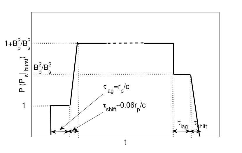
Figure 2: Illustration of the three-stage bursty light curve of an exoplanet - host star system. The first stage is caused by the stellar radiation itself which lasts a period of $\tau_{\rm lag}=d/c$; followed by the full power with contributions from both the exoplanet and the host star with $1+B_{\rm p}^{2}/B_{\rm s}^{2}$ times the power of the purely stellar emission; and ends with purely the exoplanetary radiation with power $B_{\rm p}^{2}/B_{\rm s}^{2}$ times the stellar emission, lasting for $\tau_{\rm lag}=d/c$. A shift time of $\tau_{\rm shift}\sim 0.06d/c$ (varies with the observational frequency band and the planetary magnetic field) can also be noted due to the difference of times for electrons with different Lorentz factors to reach the exoplanet.

Both the lag time $\tau_{\rm lag}$ and shift time $\tau_{\rm shift}$ are schematically shown in the light curve in Fig. 2. The magnitudes of the purely stellar (or exoplanetary) bursty radiation and the total bursty radiation, if both are well observed, can be used to estimate the ratio of the magnetic fields between the exoplanet and the host star. This light curve is achieved under the assumption that stellar synchrotron radiation occurs within the MRX site. Considering possible extensions of the length of the site producing observable radiations, the initial purely stellar radiation in Fig. 2 should not be a flat curve, but a rising curve instead. Additionally, if specific electron energy distribution is considered, the purely stellar radiation should also be a rising curve instead of a flat. However, an abrupt rise of the radiation power is still expected when the planetary radiation initiates. In order to capture the rise or decay of the flare from exoplanetary systems, an observation time longer than or comparable to the burst duration is required.

3.2 The frequency shift

As electrons with different Lorentz factors reach the exoplanet at different times, during the rising time $\tau_{\rm shift}$ of the exoplanetary emission, the radiation frequency shifts from initially the maximum value to a band with the minimum value varying with time. We first write the radiation frequency (1) in the form of the electron speed $\beta$:

$$\nu=1.3B_{\rm p}\frac{1}{1-\beta^{2}}.$$ (10)

Then using the lag time (9) to express $\beta$ in the form of the electron traveling time from the star to the planet, we have $\beta=\frac{d}{ct}$. By introducing this expression to (10) and rewrite the electron traveling time as $t=t_{0}+\tau$ with $t_{0}$ the traveling time with the speed of light, the frequency depends on the time as

$$\nu=1.3B_{\rm p}\frac{1}{1-\frac{d^{2}}{c^{2}(t_{0}+\tau)^{2}}}.$$ (11)

For relativistic electrons with the Lorentz factor greater than $\sim 2$, their speeds are smaller than the speed of light by $<10\%$; so we use the Taylor expansion in Equ. (11) for $\tau/t_{0}\ll 1$ and get the simple expression as follows:

$$\nu=1.3B_{\rm p}\frac{t_{0}}{2\tau}=\frac{1.3B_{\rm p}d}{2c}\frac{1}{\tau},$$ (12)

or in the log-normal form:

$${\rm ln}\nu={\rm ln}\big{(}\frac{1.3B_{\rm p}d}{2c}\big{)}-{\rm ln}\tau.$$ (13)

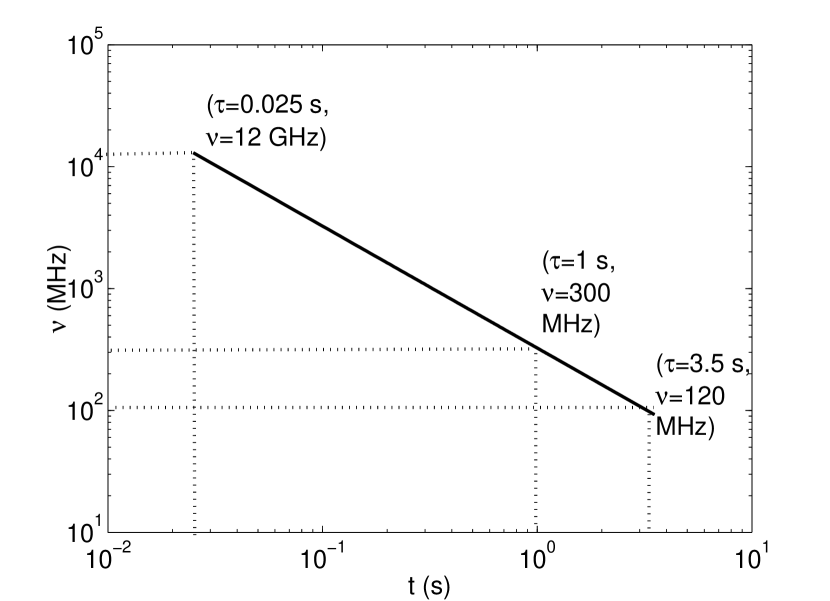
Figure 3: Frequency shift at the rising and decaying periods of the exoplanetary radio burst. A shift of the emission band minimum frequency from 12 GHz to 120 MHz occurs within 3.5 s. Observationally to be noted is the frequency at $\tau=1$ s, which can be used to calculate the degenerated planet magnetic field $B_{\rm p}$ and orbit radius $d$ according to (13).

As was indicated in the last subsection, the shift of frequency lasts about $\tau_{\rm shift}=3.5$ s to cover the range 12 GHz $>\nu>$ 120 MHz in an typical exoplanet with $B_{\rm p}=10$ G and $d=0.1$ AU. It is then readily to plot the frequency (band minimum value) - time curve describing the frequency shift at the initiation and ending phases of the exoplanetary radiation as in Fig. 3. According to Equ. (13), the frequency at time $\tau=1$ s, if well measured in observations, can be used to measure the exoplanetary magnetic field $B_{\rm p}$, where the degeneracy with $d$ may be reduced by other observations (e.g., the time-lag $\tau_{\rm lag}$). Above we calculated the continuous frequency shift at the rising and decaying periods of the exoplanetary radiation. However, the key assumption in the calculation that electrons with different Lorentz factors are produced in MRX simultaneously, may not apply in realistic MRX particle accelerations. More detailed calculations based on the time evolution of accelerated electron energy spectrum (e.g., Sironi & Spitkovsky, 2014; Matsumoto et al., 2015) may lead to different results.

There is, however, another abrupt change of frequency if we pay attention to the difference of radiation frequency at the star and the planet for electrons with the same Lorentz factor $\gamma$. In some exoplanetary systems, SPIs identified through Ca II K line activities indicate stronger planetary magnetic fields than in their host stars (Cauley et al., 2019), which is to be further confirmed in radio observations. According to (1), an increase of the maximum frequency at the burst initiation phase is expected in this kind of systems. Such frequency shift occurs at the typical time $\tau_{\rm lag}$, which is an order of magnitude longer then the frequency shift shown in Fig. 3, thus easier to be detected. When the planetary magnetic field is weaker than that of the host star, in the ending epoch an corresponding decrease of the maximum frequency is similarly expected. The abrupt shifts of the frequency then provide a measure of the magnetic field ratio $B_{\rm p}/B_{\rm s}$. This frequency shift, accompanying the power changes as shown in Fig. 2, does not relay on the evolution of the electron energy spectral during MRX, thus is a more reliable method to confirm the existence of planetary radiation. Examples of this kind of frequency shift due to the change of magnetic field can be found in type IV solar bursts, where the synchrotron frequency decreases as the energetic electrons travel out from the solar surface (Dulk, 1985); or S-bursts in the decameter emission from Jupiter (Clarke et al., 2014).

3.3 Orbital phase correlation

The features of both the light curve (rising and decaying) and the frequency shift require a good time resolution to be observationally identified. When a long integration time is required to achieve a good sensitivity for the detection of the bursts, which may last for $\sim 10^{4}$ s long, the planetary orbital phase - burst correlation can be used to identify whether the bursts have a star-planet interactions (SPI) origin.

As the stellar magnetospheres are usually not axisymmetric, both energetic plasma ejections and synchrotron emissions vary as the planet orbits around the host star. Considering the non-axisymmetry of the energetic plasma ejections from the host star, the planetary bursty emission power and rate vary and should correlate with its orbital phase in reference to a fixed local longitude of the host star. So in low-temporal-resolution observations, we suggest to plot the detection rate and/or flux density versus orbital phase diagram to help identifying the origin of bursts. Besides the orbital phase correlation as the key practical feature of planetary emissions, the synchrotron burst emission is also distinct from thermal emissions for having recognizable circular polarizations (Dulk, 1985).

4 Case study: HD 189733 b and V830 $\tau$ b

4.1 HD 189733 b

HD 189733 is a K (K1-K2) star - hot Jupiter system whose X-ray flares have been well observed by XMM-Newton, Swift and Chandra telescopes (Pillitteri et al., 2010, 2011, 2014; Lecavelier des Etangs et al., 2012; Poppenhaeger et al., 2013). Observations at the optical and FUV bands, in particular the measurement of atomic lines such as the Ca II K line, show probable interaction between the star and its planet (Pillitteri et al., 2015), and indicate a very high planetary magnetic field of 20 - 50 G (Cauley et al., 2019). According to the measured X-ray flare flux and the traditional Güdel-Benz relation, the radio flux of HD 189733 system can be estimated to be $0.01-0.09$ mJy, at a burst rate of $\sim 13\%$ with the typical burst duration of $\sim 8$ ks (Benz & Güdel, 1994, 2010; Pillitteri et al., 2014). This estimated flux, although smaller compared to the estimation of Route (2019), may reach the 0.1 mJy level if the uncertainty in the index of the Güdel-Benz relation is enlarged from 0.5 to 1. Then it is not surprising that previous radio observations give a “non-detection” result given their sensitivitis being larger than 0.3 mJy (cf. the review in Route, 2019).

For the expectation of upcoming observations, the sensitivity level of $\sim 0.1$ mJy can be achieved by a $\sim 100$-seconds integration with VLA at 4.5 GHz with 1 GHz bandwidth (Bower et al., 2016), or $\sim 300$-seconds integration with FAST at 1.4 GHz with 400 MHz bandwidth (Li et al., 2019). Achieving a sensitivity of a few $0.01$ mJy by increasing the integration time to the ks level is also possible. However, to distinguish the HD 189733 emission from the Galactic background, the confusion limit of FAST (Zhang et al., 2018b) needs to be increased simultaneously to the $0.01$ mJy level by using a short baseline interferometer to reduce the main-beam-width to $\sim$ 10 arc-seconds level (cf. Zarka et al., 2019). For the detection rate, given a burst rate of $13\%$ with the burst duration of $\sim 8$ ks, a single observation with integration time of 8 ks has $23\%$ chance to capture the burst, if we consider that a $\sim$ 1 ks integration time is required to achieve the sensitivity of a few $0.01$ mJy. Then a detectability of $93\%$ is expected in ten observations with each having 8 ks integration time.

However, such long integration time of kilo-seconds makes it impossible to temporally resolve the flux variation and frequency shift at $\tau_{\rm lag}=50$ s as shown in Section 3. Such features can only be captured using the SKA2 for flares at 0.05 mJy level, or SKA1 for flares at 0.5 mJy level (cf. Pope et al., 2019).

Given the large number of nearby ($\sim 10$ pc) young, late type (K and M) stars with exoplanets discovered, the detection of radio flares at a flux similar to the estimation of HD 189733 is expected on VLA and FAST (with reduced confusion limits). Such observational attempts will be more efficient if proper selections from the sources with X-ray flares already detected are made (e.g., Maggio et al., 2015).

4.2 V830 $\tau$ b

For the T Tauri star V830 $\tau$, the radio flare detection is even before the confirmation of the existence of a hot Jupiter around it (Donati et al., 2016, 2017; Bower et al., 2016). Detected by VLA and VLBI among the five observations in two separated epoches, the radio flux is $\sim 0.5$ mJy, with a burst rate of $\sim 40\%$ (Bower et al., 2016). Compared to HD 189733, an observational sensitivity at 0.1 mJy level (100-seconds VLA integration, or 300-seconds FAST integration without confusion from the background within the main-beam) should be good enough to detect such bursts. Being lack of the information about the duration time of the bursts, we assume them to be much longer than the $\sim$300 s integration time of existing VLA observations; consequently a $40\%$ chance of detection for a single observation lasting 300 s is expected, and the detectability is $92\%$ in five observations. To further capture the rising and ending light curves of a burst, a longer single observation time of a few kilo-seconds is required, consequently a higher detection rate is expected.

The flux change that occurs $\tau_{\rm lag}=50$ seconds after the burst initiation, as well as the accompanying abrupt frequency shift are expected to be observed by SKA1 at a sensitivity of 0.1 mJy for 5-seconds integration (Pope et al., 2019). The continuous frequency shift within $\tau_{\rm shift}\sim 3.5$ s at the initiation of the planetary radiation is also expected to be resolved by SKA2 with its sensitivity better than SKA1 by an order of magnitude.

There are quite a number of T-Tauri stars with radio flare flux densities similar to V830 $\tau$ (White et al., 1992; Feigelson et al., 1994; Suters et al., 1996). Although only a small portion of them have been detected bearing exoplanets due to the selection bias of current methods, the commonly existence of planets or protoplanets around T-Tauri stars is expected. Then observations toward T-Tauri stars, as well as other K and M type stars with strong flares, will possibly detect the radio flare - (unknown) planetary orbital phase correlation, which may serve as a new method of exoplanet discovery.

5 Conclusion and discussions

Scaling analysis and applications to specific sources show that for the detection of exoplanetary synchrotron radio bursts from K and T-Tauri stars hosting planets, current telescopes VLA, FAST and Arecibo (with necessary interferometers to reduce the confusion limit for the later two) have the required sensitivity of a few $0.01$ mJy given enough integration time. To resolve the signatures of both the flux variation and the frequency shift at the rising and ending processes of the burst (Fig. 2 and Section 3) in order to identify emissions from the exoplanet, SKA has the required sensitivity. Before SKA, with the increasing number of radio detections from star-exoplanet systems, the orbital phase - burst correlation may serve as a prior way to discuss whether the radio emission is related with SPI (Pillitteri et al., 2014; Maggio et al., 2015; Route, 2019). For the selection of targets, systems with stronger host stellar magnetic field ($>\sim 100$ G) are expected to have higher electron transportation efficiency from the star to the planet, thus have stronger planetary synchrotron bursts.

M dwarfs and ultra cool dwarfs (UCD) are also radio active stars with their flare strength comparable to or stronger than K stars (Dulk, 1985; Hughes et al., 2019). In the TESS era, the detection of hundreds of M dwarfs with optical flares provides a pool for further radio observations (Günther et al., 2020; Doyle et al., 2019). M dwarfs may host nearby planets either with strong magnetic fields, or without magnetic fields but electrically conductive. The former systems are expected to have similar synchrotron radio bursts as was discussed in this paper; while the radiation features of flares from conductive exoplanets around M dwarfs is beyond the scope of this paper.

References

- Abada-Simon (1996) Abada-Simon, M. 1996, Plant. Space Sci., 44, 501
- Audard et al. (2000) Audard M, Güdel, M., Drake, J. J. & Kashyap, V. L. 2000, ApJ, 541, 396
- Bastian et al. (2000) Bastian, T. S., Dulk, G. A. & Leblanc, Y. 2000, ApJ, 545, 1087
- Becker et al. (2017) Becker, H. N., Santos-Costa, D., Jørgensen, J. L., Denver, T., Adriani A., et al. 2017, Geophys. Res. Lett., 44, 4481
- Benz & Güdel (1994) Benz, A. O. & Güdel, M. 1994, A&A, 285, 621
- Benz & Güdel (2010) Benz, A. O. & Güdel, M. 2010, ARA&A, 48, 241
- Bhardwaj et al. (2009) Bhardwaj, A., Ishwara-Chandra, C. H., Shankar, N. U., Misawa, H., Imai, K. 2009, in The Low-Frequency Radio Universe (Saikia, D. J., Green, D. A., Gupta, Y. and Venturi, T. eds., ASP Conference Series, Vol. 407, p.369-372)
- Bower et al. (2016) Bower, G. C., Loinard, L., Dzib, S., Galli, P. A. B., Ortiz-León, G. N., Moutou, C. & Donati, J.-F. 2016, ApJ, 830, 107
- Cauley et al. (2019) Cauley, P. W., Shkolnik, E. L., Llama, J. & Lanza, A. F. 2019, Nat. As., 3, 1128
- Chadney et al. (2017) Chadney, J. M., Koskinen, T. T., Galand, M., Unruh, Y. C. & Sanz-Forcada, J. 2017, A&A 608, A75
- Clarke et al. (2014) Clarke, T. E., Higgins, C. A., Skarda, J., Imai, K., Imai, M. et al. 2014, Journal of Geographysical Research: Space Physics, 119, 12
- Crosby et al. (1993) Crosby, N. B., Aschwanden, M. J. & Dennis, B. R. 1993, Solar Phys. 143, 275
- de Pater (2004) de Pater, I. 2004, Planet. Space Sci., 52, 1449
- Donati et al. (2016) Donati, J. F., Moutou, C., Malo, L., Baruteau, C., Yu, L. et al. 2016, Nature, 534, 662
- Donati et al. (2017) Donati, J. F., Yu, L., Moutou, C., Camero, A. C., Malo, L. et al. 2017, MNRAS, 465, 3343
- Doyle et al. (2019) Doyle, L., Ramsay, G., Doyle, J. G. & Wu, K. 2019, MNRAS, 489, 437
- Dulk (1985) Dulk, G. A. 1985, ARA&A, 23, 169
- Feigelson et al. (1994) Feigelson, E. D., Welty, A. D., Imhoff, C., Hall, J. C., Etzel, P. B., Phillips, R. B. & Lonsdale, C. J. 1994, ApJ, 432, 373
- Girard et al. (2016) Girard, J. N., Zarka, P., Tasse, C., Hess, S., de Pater, I. et al. 2016, A&A, 587, A3
- Grießmeier (2006) Grießmeier, J.-M. 2006, Doktors der Naturwissenschaften,
- Grießmeier (2016) Grießmeier, J.-M. 2016, in Planetary Radio Emissions VIII, Proceedings of the 8th International Workshop (Fischer, G., Mann, G., Panchenko, M., and Zarka, P. eds. Austrian Academy of Sciences Press, Vienna, 2017, p. 285-299)
- Güdel et al. (2003) Güdel, M., Audard M., Drake J. J., Kashyap, V. L. & Guinan, E. F. 2003, ApJ, 582, 423
- Günther et al. (2020) Günther, M. N., Zhan, Z., Seager, S. et al. 2019, AJ, 159, 60
- Hughes et al. (2019) Hughes, A. G., Boley, A. C., Osten, R. A. & White J. A. 2019, ApJ, 881, 33
- Isobe et al. (2005) Isobe, H., Takasaki, H. & Shibata, K. 2005, ApJ, 632, 1184
- Ji & Daughton (2011) Ji, H. & Daughton, W. 2011, Phys. Plasmas, 18, 111207
- Kloosterman et al. (2008) Kloosterman, J. L., Butler, B. & de Pater, I. 2008, Icarus, 193, 644
- Lanza (2018) Lanza, A. F. 2018, A&A, 610, A81
- Lecavelier des Etangs et al. (2012) Lecavelier des Etangs, A., Bourrier, V., Wheatley, P. J., Dupuy, H., Ehrenreich, D., et al., 2012, A&A, 543, L4
- Li et al. (2019) Li, D., Dickey, J. M., & Liu, S. 2019, RAA, 19, 16
- Lou et al. (2012) Lou, Y.-Q., Song, H., Liu, Y. & Yang, M. 2012, MNRAS, 421, 62
- Lynch et al. (2018) Lynch, C. R., Murphy, T., Lenc, E. & Kaplan, D. L. 2018, MNRAS, 478-1763
- Maggio et al. (2015) Maggio, A., Pillitteri, I., Scandariato, G., Lanza, A. F., Sciortino, S. et al. 2015, ApJL, 811, L2
- Manser et al. (2019) Manser, C. J., Gänsicke, B. T., Eggl, S. et al. 2019, Science, 364, 66
- Matsumoto et al. (2015) Matsumoto, Y., Amano, T., Kato, T. N. & Hoshino, M. 2015, Science, 347, 974
- Mutel et al. (1985) Mutel, R. L., Lestrade, J. F., Preston, R. A. & Phillips, R. B. 1985, ApJ, 289, 262
- Pillitteri et al. (2010) Pillitteri, I., Wolk, S. J., Cohen, O., Kashyap, V., Knutson, H., Lisse, C. M. & Henry, G. W. 2010, ApJ, 722, 1216
- Pillitteri et al. (2011) Pillitteri, I., Günther, H. M., Wolk, S. J.,, Kashyap, V. L. & Cohen, O. 2011, ApJL, 741, L81
- Pillitteri et al. (2014) Pillitteri, I., Wolk, S. J., Lopez-Santiago, J., Günther, H. M., Sciortino, S., Cohen, O., Kashyap, V., & Drake, J. J. 2014, ApJ, 785, 145
- Pillitteri et al. (2015) Pillitteri, I., Maggio, A., Micela, G., Sciortino, S., Wolk, S. J. & Matsakos, T. 2015, ApJ, 805, 52
- Pope et al. (2019) Pope, B. J. S., Withers, P., Callingham, J. R. & Vogt, M. F. 2019, MNRAS, 484, 648
- Poppenhaeger et al. (2013) Poppenhaeger, K., Schmitt, J. H. M. M., & Wolk, S. J. 2013, ApJ, 773, 62
- Route (2019) Route, M. 2019, ApJ, 872, 79
- Reiners & Christensen (2010) Reiners, A. & Christensen, U. R. 2010, A&A, 522, A13
- Rybicki & Lightman (1979) Rybicki, G. B. & Lightman A. P. 1979, Radiative Processes in Astrophysics, John Wiley & Sons
- Sirothia et al. (2014) Sirothia, S. K., Lecavelier des Etangs, A., Gopal-Krishna, Kantharia, N. G., & Ishwar-Chandra, C. H. 2014, A&A 562, A108
- Sironi & Spitkovsky (2014) Sironi, L. & Spitkovsky, A. 2014, ApJL, 783, L21
- Stelzer et al. (2007) Stelzer, B., Flaccomio, E., Briggs, K. et al. 2007, A&A, 468, 463
- Suters et al. (1996) Suters, M., Stewart, R. T., Brown, A. & Zealey, W. 1996, ApJ, 111, 320
- Trigilio et al. (2018) Trigilio, C., Umana, G., Cavallaro, F., Agliozzo, C., Leto P., et al. 2018, MNRAS, 481, 217
- Uchida & Sakurai (1983) Uchida, Y. & Sakurai, T. 1983, in P. B. Byrne & M. Ronodo (eds.), Activaty of Red Dwarf Stars, p. 629
- Vanderburg et al. (2015) Vanderburg, A., Johnson, J. A., Rappaport, S. et al. 2015, Nature, 526, 546
- Vidotto & Donati (2017) Vidotto, A. A. & Donati, J.-F. 2017, A&A, 602, A39
- Wang & Loeb (2019) Wang, X. & Loeb A. 2019, ApJ, 874L, 23
- White et al. (1992) White, S. M., Pallavicini, R. & Kundu, M. R. 1992, A&A, 257, 557
- Willes & Wu (2005) Willes, A. J. & Wu, K. 2005, A&A, 432, 1091
- Wu & Lee (1979) Wu, C. S. & Lee, L. C. 1979, ApJ, 230, 621
- Yamada et al. (2010) Yamada, M., Kulsrud, R. & Ji, H. 2010, Rev. Mod. Phys. 82, 603
- Yantis et al. (1977) Yantis, W. F., Sullivan, III., W. T. & Erickson, W. C. 1977, Bull Am. Astron. Soc., 9, 453
- Zarka et al. (2015) Zarka, P., Lazio, T. J. W., Hallinan, G. & ”Cradle of Life” WG 2015, in Advancing Astrophysics with the Square Kilometre Array (Proceedings of Science (AASKA14) 120)
- Zarka et al. (2019) Zarka, P., Li, D., Grießmeier, J.-M., Lamy, L., Girard, J. N., Hess, S. L. G., Lazio, T. J. W. & Hallinan, G. 2019, RAA, 19, 23
- Zhang et al. (2018) Zhang, H., Gao, Y. & Law, C. K. 2018, ApJ, 864, 167
- Zhang et al. (2018b) Zhang, Z. B., Chandra, P., Huang, Y. F. & Li, D. 2018, ApJ, 865, 82
- Zweibel & Yamada (2009) Zweibel, E. G. & Yamada, M. 2009, ARA&A, 47, 291