State Dependence and Unobserved Heterogeneity
in the Extensive Margin of Trade

Abstract

We study the role and drivers of persistence in the extensive margin of bilateral trade. Motivated by a stylized heterogeneous firms model of international trade with market entry costs, we consider dynamic three-way fixed effects binary choice models and study the corresponding incidental parameter problem. The standard maximum likelihood estimator is consistent under asymptotics where all panel dimensions grow at a constant rate, but it has an asymptotic bias in its limiting distribution, invalidating inference even in situations where the bias appears to be small. Thus, we propose two different bias-corrected estimators. Monte Carlo simulations confirm their desirable statistical properties. We apply these estimators in a reassessment of the most commonly studied determinants of the extensive margin of trade. Both true state dependence and unobserved heterogeneity contribute considerably to trade persistence and taking this persistence into account matters significantly in identifying the effects of trade policies on the extensive margin.

JEL Classification Codes: C13, C23, C55, F14, F15
Key Words: Dynamic binary choice, extensive margin, high-dimensional fixed effects, incidental parameter bias correction, trade policy

1 Introduction

What induces country pairs to trade? In 2019, still more than one third of potential bilateral trade relations reported zero trade flows. Comparing these zero trade flows with trade relations in 2018, these zeros turn out to be extremely persistent: 88.6 percent of country pairs that did not trade in 2018 did not trade in 2019 either, as can be seen in the transition matrix depicted in Table 1. And similarly, 92.3 percent of pairs that did trade in 2018 continued to do so in the year after.

Table 1: Persistence in Bilateral Trade Relations (2018 – 2019)

	Traded in 2019
Traded in 2018	No	Yes
No	88.6 %	11.4 %
Yes	7.7 %	92.3 %

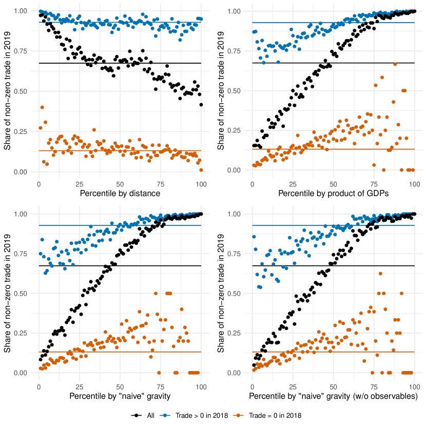
Figure 1: Determinants of the Extensive Margin of Trade — Gravity and Persistence.

Note: Trade data for 2018 – 2019 come from UN Comtrade, GDP, distances and gravity variables are sourced from CEPII [13].

Both intuitively and based on existing theoretical and empirical insights, we would expect geographically close and economically large country pairs to have the greater bilateral trade potential and thus be more likely to engage in international trade. As distance is time-invariant and economic size does not change abruptly from one year to another, these gravity-like characteristics may explain (part of) the observed persistence. Figure 1 breaks down the share of non-zero trade flows in 2019 along the percentiles of four different ad hoc indicators of trade potential: bilateral distance; product of GDPs; “naive” gravity, i.e. the product of GDPs divided by the countries’ bilateral distance; and the latter when excluding country pairs in FTAs, with common currencies or common colonial history. The x-axis indicates the potential trade volume, i.e. the joint economic size and/or proximity of any two countries. All four plots paint a common picture: the black dots, covering all country pairs, show a strong general relationship between trade potential and actual non-zero trade. The blue and red dots split the country pairs according to whether the two did or did not engage in trade in the previous year. The clearly separated pattern for the two groups highlights the remarkable persistence of trade relations, even after controlling for differences in trade potential in terms of distance, size, and bilateral trade policy. More than 50 percent of those country pairs in the lowest percentiles of trade potential trade again in 2019, provided they already did so in 2018. On the other hand, even comparably large and close pairs are likely not to trade in 2019 if they did not trade in 2018 either.

Two potential features of the extensive margin of trade that can generate the pattern documented by Table 1 and Figure 1 are what [34] termed “true state dependence” and “spurious state dependence”. The former characterizes countries to actually be more likely to trade because they did so in the previous period, whereas the latter describes persistence due to unobservable factors continuously driving bilateral trade potential.

In this paper we introduce estimators for the determinants of the extensive margin of international trade that explicitly take its persistence due to observable characteristics, true state dependence, and unobserved heterogeneity into account. We introduce features from the firm dynamics literature into a heterogeneous firms model of international trade with bounded productivity to derive expressions for an exporting country’s participation in a specific destination market in a given period. These expressions depend on partly unobserved (i) exporter-time, (ii) destination-time, and (iii) exporter-destination specific components, as well as on (iv) whether the exporter has already served the market in the previous period, and on (v) exporter-destination-time specific gravity-type trade cost determinants. We estimate the model making use of recent computational advances in the estimation of binary choice estimators with high-dimensional fixed effects to address (i)-(iii). The inclusion of fixed effects in a binary choice setting induces an incidental parameter problem that is potentially aggravated by the dynamics introduced by (iv). To mitigate this bias, we propose new analytically and jackknife bias-corrected estimators for coefficients and average partial effects in three-way fixed effects specifications. Additionally, we provide an expression for long-run partial effects. Extensive simulation experiments demonstrate the desirable statistical properties of our proposed bias-corrected estimators.

The empirical application provides evidence that both unobserved bilateral factors and true state dependence due to entry dynamics contribute strongly to the high persistence. Taking this persistence into account changes the estimated effects of the most commonly studied potential determinants considerably: The impact of a common currency is reduced from almost 10 percentage points to less than 4 percentage points, the effect of a common regional trade agreement drops from 5.4 to 1.2 percentage points, and joint membership in the WTO/GATT increases the trading probability by 1.3 rather than 3.4 percentage points. For all three variables, only about two thirds of these effects are realized immediately, while the remaining third is added gradually over time. Furthermore, specifications with a lagged dependent variable and/or bilateral fixed effects yield better predictions for which country pairs will trade than specifications that fail to account for state dependence appropriately.

Our paper builds on recent insights from three flourishing strands of literature. First, our paper is related to the literature on the extensive margin of international trade. A number of theoretical frameworks have sought to propose mechanisms behind the decisions of firms to export, and their aggregate implications of zero or non-zero trade flows at the country pair level. Analogous to the intensive margin counterpart, these theories have established gravity-like determinants, such as two countries’ bilateral distance, a free trade agreement, a common currency and joint membership in the WTO/GATT. [21] and [22] append an extensive margin to an [2]-type model by assuming export participation to be determined by (homogeneous) firms weighing operating profits and bilateral fixed costs of exporting. [35] build a model of international trade with heterogeneous firms and bounded productivity in which a country only exports to a given destination if the most productive firm can afford to overcome the fixed costs of exporting. [20] move away from the arguably simplifying notion of a continuum of firms and develop a model of a finite set of heterogeneous firms. Here, no firm may export to a given market because of their individual efficiency draws. Our model proposed in this paper directly builds on [35] and extends it by features from the literature on firm dynamics. In this firm-level literature, [16] develop a dynamic discrete-choice model in which current export participation depends on previous exporting, and hence sunk costs, and observable characteristics of profits from exporting [42, 9, in line with previous empirical evidence by]. [1] embed the distinction between sunk costs and “period-by-period” fixed costs into general equilibrium. We aim at reconciling the estimation of the aggregate extensive margin with the insight from the firm-level literature that dynamics feature prominently in the determination of the exporting decision by deriving an econometric specification that explicitly incorporates previous export experience at the country pair level.

Second, our paper builds on advances in the literature on the gravity equation and the intensive margin of international trade. With the advent of what has now been coined structural gravity [32], the gravity framework has gained rich microfoundations. [2] and [18] each formulate an underlying structure for exporting and importing countries that in estimations can easily be captured by appropriate two-way country(-time) fixed effects, as first noted by [23] and [41]. Since [4], it has furthermore become standard to include country pair fixed effects to tackle unobservable bilateral trade cost determinants. Additionally taking into account the multiplicative structure of the gravity equation following [44], nonlinear estimation with exporter-time, importer-time, and country pair fixed effects has become the gold standard for the intensive margin. Estimating the model introduced in this paper similarly calls for three sets of fixed effects, specific to exporters and importers in a given year, as well as to a given country pair over time. The binary nature of the decision whether to export to a destination market at all, also clearly asks for a nonlinear estimator. Therefore, in this paper, we put the estimation of the extensive margin on a par with the intensive margin gold standard by introducing a respective three-way fixed effects binary choice specification.

Third, the paper builds on and contributes to the literature on estimating nonlinear fixed effects models. As it is known since [38], the inclusion of fixed effects potentially introduces an incidental parameter problem (IPP). Although the maximum likelihood estimator (MLE) is consistent if all dimensions of the panel grow large, it has an asymptotic bias in its limiting distribution leading to invalid inference [25, see]. Recently, there have been a number of advances to deal with the IPP [25, see]. In the context of the aggregate extensive margin, only approaches for cross-sectional bilateral data with importer ($j$) and exporter ($i$) fixed effects have been suggested. [14] apply the bias correction of [24], and [12] proposes a conditional logit estimator. Many trade data sets however consist of bilateral cross-sections over time, i.e. network panel data. The theory-consistent estimation of our model includes fixed effects for exporter-time ($it$) and importer-time ($jt$). On closer inspection, one finds that this two-way case can basically be covered by the bias corrections of [24] for individual and time fixed effects. However, the literature lacks a suitable method to estimate our preferred specification, which additionally includes a third, bilateral ($ij$), set of fixed effects. Our contribution is to develop suitable three-way fixed effects binary choice estimators for network panel data with potentially weakly exogeneous regressors under asymptotics where $I,J$ and $T$ are large. Therefore, our article complements the work of [48] on estimating the intensive margin of trade, who examine the IPP for the three-way fixed effects Poisson pseudo maximum likelihood (PPML) estimator under fixed $T$ asymptotics and suggest appropriate bias corrections.

The remainder of the paper is structured as follows. In Section 2 we build a dynamic model of the extensive margin of international trade. The model yields aggregate predictions that can be structurally estimated using a probit model with high-dimensional fixed effects. In Section 3 we describe the new bias-corrected three-way fixed effects estimator. We demonstrate its performance in Monte Carlo simulations in Section 4, before finally showing the estimator in action by estimating the model in Section 5. Section 6 concludes.

2 An Empirical Model of the Extensive Margin of Trade

We start by setting up a model of the extensive margin of trade that will later guide our econometric specification. We consider a stylized dynamic [37]-type heterogeneous firms model of international trade. Following [35] we assume a bounded productivity distribution, like a truncated Pareto in HMR’s case. We deviate from HMR by explicitly stating a time dimension and, unlike in the standard Melitz setting, separate fixed exporting costs into costs of entering a new market and costs of selling in a given market [1, 16, as in].

There are $N$ countries, indexed by $i$ and $j$, each of which consumes and produces a continuum of products. The representative consumer in $j$ receives utility according to a CES utility function:

$$u_{jt}=\left(\int_{\omega\in\Omega_{jt}}(\xi_{ijt})^{\frac{1}{\sigma}}q_{jt}(\omega)^{\frac{\sigma-1}{\sigma}}d\omega\right)^{\frac{\sigma}{\sigma-1}}\quad\text{with}\quad\sigma>1.$$ (1)

where $q_{jt}(\omega)$ is $j$’s consumption of product $\omega$ in period $t$, $\Omega_{jt}$ is the set of products available in $j$, $\sigma$ is the elasticity of substitution across products, and $\xi_{ijt}$ is a log-normally distributed idiosyncratic demand shock (with $\mu_{\xi}=0$ and $\sigma_{\xi}=1$) for goods from country $i$ in country $j$ and period $t$ [19, similar to]. Demand in country $j$ for good $\omega$ depends on this demand shock, $j$’s overall expenditure $E_{jt}$, and the good price $p_{jt}(\omega)$ relative to the overall price level as captured by the price index $P_{jt}$:

$$q_{jt}(\omega) =\frac{p_{jt}(\omega)^{-\sigma}}{P_{jt}^{1-\sigma}}\xi_{ijt}E_{jt}.$$

$$\text{with}\qquad P_{jt} =\left(\int_{\omega\in\Omega_{jt}}\xi_{ijt}p_{jt}(\omega)^{1-\sigma}d\omega\right)^{\frac{1}{1-\sigma}}\,.$$

Each country has a fixed continuum of potentially active firms that have different productivities drawn from the distribution $G_{it}(\varphi)$, where $\varphi\in(0,\varphi_{it}^{*}]$. The productivity distribution evolves over time and firms’ ranks within the productivity distribution can also change from period to period, though firms that in the last period did not export to a market already served by a domestic competitor are assumed not to directly jump to being the country’s most productive firm in the next period. Each period, a firm can decide to pay a fixed cost $f_{it}^{prod}$ and start production of a differentiated variety using labour $l$ as its only input, such that $l_{t}(\omega)=f_{it}^{prod}+q_{t}(\omega)/\varphi_{t}(\omega)$. A firm’s marginal cost of providing one unit of its good to market $j$ consists of iceberg trade costs $\tau_{ijt}$ and labour costs $w_{it}/\varphi_{t}(\omega)$. Firms compete with each other in monopolistic competition and charge a constant markup over marginal costs. Therefore, the price of a good $\omega$ produced in $i$ and sold in $j$ is:

$$p_{ijt}(\omega)=\frac{\sigma}{\sigma-1}\frac{\tau_{ijt}w_{it}}{\varphi_{t}(\omega)}.$$

A firm’s operating profits in market $j$ are hence given by:

$$\tilde{\pi}_{ijt}(\omega)=\frac{1}{\sigma}\left(\frac{\sigma}{\sigma-1}\frac{\tau_{ijt}w_{it}}{\varphi_{t}(\omega)}\right)^{1-\sigma}P_{jt}^{\sigma-1}\xi_{ijt}E_{jt}.$$

If a firm wants to export to a market $j$ in period $t$, it has to pay a fixed exporting cost $f_{ijt}^{exp}$. The exporting fixed cost is higher by a market entry cost factor $f^{entry}\geq 1$ if the firm has not been active in the respective market in the previous period. For tractability, the entry cost factor is assumed to be constant across countries and time. Capturing the export decision by a binary variable $y_{ijt}(\omega)$, i.e. equal to one if the firm decides to serve market $j$ in period $t$, we can formalize a firm’s realized profits in market $j$ as follows:

$$\pi_{ijt}(\omega)=y_{ijt}(\omega)\left\{\tilde{\pi}_{ijt}(\omega)-f_{ijt}^{exp}(f^{entry})^{[1-y_{ij(t-1)}(\omega)]}\right\}.$$

In the absence of entry costs, a firm would simply compare its operating profits to the fixed exporting cost and decide to serve a market if the former are greater than the latter. With market entry costs, a firm might be willing to incur a loss in the current period if expected future profits from that same market outweigh the initial loss. Firms discount future profits at a rate $\delta$ per period. To keep things tractable and allow us to derive a theory-consistent estimation expression below, we assume that firms expect their future operating profits from and fixed costs of serving a given market to be equal to today’s values, i.e. $\operatorname{\mathbb{E}}_{t}[\tilde{\pi}_{ij(t+s)}]=\tilde{\pi}_{ijt}$ and $\operatorname{\mathbb{E}}_{t}[f^{exp}_{ij(t+s)}]=f^{exp}_{ijt}$ $\forall s\in\mathbb{N}$. The current value of today’s and all future operating profits from market $j$ is then given by $\sum_{s=0}^{\infty}(1-\delta)^{s}\tilde{\pi}_{ijt}=\frac{\tilde{\pi}_{ijt}}{\delta}$. A firm will decide to serve a destination market if these discounted expected profits exceed the sum of today’s and discounted future fixed costs of entry and exporting, given by

$$f^{exp}_{ijt}(f^{entry})^{(1-y_{ij(t-1)}(\omega))}+\sum_{s=1}^{\infty}(1-\delta)^{s}f^{exp}_{ijt}=\frac{f^{exp}_{ijt}}{\delta}\left(1+\delta(f^{entry}-1)\right)^{(1-y_{ij(t-1)}(\omega))}\,.$$

Given this model setup, the question whether a country exports to another country at all can be considered by looking at the most productive firm (with $\varphi_{t}^{*}$) only. Denoting that firm’s product by $\omega^{*}$, we can capture the aggregate extensive margin by the binary variable $y_{ijt}$ as follows:

$$y_{ijt}=y_{ijt}(\omega^{*})=\begin{cases}1\quad\text{if}\quad\frac{\left(\frac{1}{\sigma}\left(\frac{\sigma}{\sigma-1}\frac{\tau_{ijt}w_{it}}{\varphi_{it}^{*}}\right)^{1-\sigma}P_{jt}^{\sigma-1}\xi_{ijt}E_{jt}\right)}{f_{ijt}^{exp}\left(1+\delta(f^{entry}-1)\right)^{(1-y_{ij(t-1)})}}\geq 1,\\ 0\quad\text{else}.\end{cases}$$ (2)

Country $i$ is hence more likely to export to country $j$ in period $t$ if (i) bilateral variable trade costs are lower; (ii) wages in $i$, and hence production costs, are lower; (iii) the productivity of the most productive firm is higher, again reducing production costs; (iv) competitive pressure, inversely captured by the price index, in $j$ is lower, corresponding to the idea of inward multilateral resistance coined by [2] in the intensive margin context; (v) the market in $j$ is larger; (vi) bilateral fixed costs of exporting are smaller; or (vii) $i$’s most productive firm already served market $j$ in the previous period and therefore does not have to pay the market entry cost. Note that (i) to (iv) all act via higher operating profits and depend on the elasticity of substitution between goods. The higher this elasticity, the stronger the reaction of profits to changes in any of these factors. At the same time, a higher elasticity reduces the mark-up firms can charge and hence makes it generally harder to earn enough profits to mitigate the fixed costs of exporting. Further note that the importance of the entry costs depends on the discount factor. Intuitively, if agents are more patient, the one-time entry costs matter less compared to the repeatedly earned profits. Empirically, (vii) induces true state dependence. As previous exporters do not have to incur entry costs, they are more likely to stay active in the destination market and the extensive margin becomes more persistent than would be implied merely by the persistence of productivity, market potential, and trade costs.

In order to turn equation (2) into the empirical expression that we will bring to the data, we take the natural logarithm and group all exporter-time and importer-time specific components and capture them with corresponding sets of fixed effects. Further, we need to specify the fixed and variable trade costs. In keeping with the existing literature, we model them as a linear combination of different observable bilateral variables, such as geographic distance, whether $i$ and $j$ are both WTO/GATT members, and whether $i$ and $j$ share a common currency. In our most general specification, we additionally include country pair fixed effects. Following [4], this is common practice in the estimation of the determinants of the intensive margin of trade in order to avoid endogeneity due to unobserved heterogeneity. Further, these bilateral fixed effects may capture (part of) the strong persistence documented above. Note, however, that the nature of the persistence captured by these fixed effects is different from the one that is due to the entry dynamics. This additional state dependence is “spurious” in the sense that countries are not actually more likely to export to a destination because of the prior experience, but because they keep incorporating the same unobserved factors over time. With the three sets of fixed effects and our parametrization for time-varying trade cost determinants, we arrive at the following econometric model:

$$y_{ijt}=\begin{cases}1\quad\text{if}\quad\kappa+\lambda_{it}+\psi_{jt}+\beta_{y}y_{ij(t-1)}+\mathbf{z}_{ijt}^{\prime}\mbox{\boldmath${\beta}$}_{z}+\mu_{ij}\geq\zeta_{ijt},\\ 0\quad\text{else},\end{cases}$$ (3)

where $\kappa=-\sigma\log(\sigma)-(1-\sigma)\log(\sigma-1)-\log(1+\delta(f^{entry}-1))$, $\lambda_{it}=(1-\sigma)(\log(w_{it})-\log(\varphi_{it}^{*}))$, $\psi_{jt}=(\sigma-1)\log(P_{jt})+\log(E_{jt})$, $\beta_{y}=\log(1+\delta(f^{entry}-1))$, $\mathbf{z}_{ijt}^{\prime}\mbox{\boldmath${\beta}$}_{z}+\mu_{ij}=(1-\sigma)\log(\tau_{ijt})-\log(f_{ijt}^{exp})$, and $\zeta_{ijt}=-\log(\xi_{ijt})\sim\mathcal{N}(0,1)$. The error term distribution implies that a probit estimator is the appropriate choice to estimate our model. Alternatively, we could deviate from [19] and assume a log-logistic distribution for the idiosyncratic demand shocks, which would lead to a logit specification. As mentioned above, we capture the three sets of unobserved components by introducing according sets of fixed effects. A supposed alternative using random effects is actually not possible, at least for the $it$ and $jt$ effects, as they are implied by the theoretical model. We therefore cannot make the distributional assumptions required in a random effects setting. The theory is silent about the exact form of the bilateral heterogeneity. We decide for a third set of fixed effects as the most general option in order to avoid assumptions on its distribution or its correlation to observed factors.

Our theoretical framework implies a flexible empirical specification that can reconcile the extensive margin estimation with the stylized fact presented in Section 1. Note that we chose to make a number of simplifying assumptions in order to achieve the clear theory-consistent interpretation of specification (3). An alternative interpretation of equation (3) as a reduced-from representation of a more elaborate and realistic model [42, similar e.g. to how] is equally justifiable. At the same time, while our model is written along the lines of [35], which remains the benchmark for the empirical assessment of the (aggregate) extensive margin of trade, it is not decisive for our empirical specification that zero trade flows result from a truncated productivity distribution instead of a discrete number of firms [20, as in] or from fixed exporting costs in a [36]-type homogeneous firms setting [21, 22, as in].

3 Binary Choice Estimators with Three-Way Fixed Effects

Having set up the empirical framework, we now turn to the estimation. As equation (3) demands three-way fixed effects to capture unobservable characteristics, we describe how to implement suitable binary choice estimators. In a first step, we review the standard maximum likelihood estimator (MLE) for probit and logit models with fixed effects. In a second step, we explain the consequences of the incidental parameter problem on the MLE and characterize new bias corrections to address the induced incidental parameter problem.

3.1 Model and Maximum Likelihood Estimation

Our empirical model (3) can be be written in a general way by the following three-way fixed effects binary choice model:

$$y_{ijt}=1(\mathbf{x}_{ijt}^{\prime}\mbox{\boldmath${\beta}$}+\psi_{jt}+\lambda_{it}+\mu_{ij}\geq\zeta_{ijt}),\qquad\zeta_{ijt}\mid\mathbf{x}_{ij}^{t},\bm{\psi},\bm{\lambda},\bm{\mu}\sim F_{\zeta}$$ (4)

where $i=1,\dots,I$, $j=1,\dots,J$, and $t=1,\dots,T$ are the indexes denoting exporters, importers, and time periods, respectively, $\mathbf{x}_{ijt}$ is a $p$-dimensional vector of regressors, ${\beta}$ are the corresponding structural parameters, $\bm{\psi}=(\psi_{11},\dots,\psi_{JT})$, $\bm{\lambda}=(\lambda_{11},\dots,\lambda_{IT})$, and $\bm{\mu}=(\mu_{11},\dots,\mu_{IJ})$ are the incidental parameters, $\mathbf{x}_{ij}^{t}=(\mathbf{x}_{ijt},\mathbf{x}_{ij(t-1)},\dots,\mathbf{x}_{ij1})$, and $F_{\zeta}$ is either the logistic or standard normal cumulative distribution function. Note that we allow $\mathbf{x}_{ijt}$ to contain weakly exogenous regressors. This is important, because our empirical model (3) contains a lagged dependent variable, which violates the strict exogeneity condition, i.e. $\zeta_{ijt}\mid\mathbf{x}_{ij}^{T},\bm{\psi},\bm{\lambda},\bm{\mu}\sim F_{\zeta}$ with $\mathbf{x}_{ij}^{T}=(\mathbf{x}_{ijT},\mathbf{x}_{ij(T-1)},\dots,\mathbf{x}_{ij1})$. Even in the absence of a lagged dependent variable, the strict exogeneity condition is often too restrictive, since it rules out any dynamic feedback between regressors and the dependent variable.

A standard estimator for the parameters of interest ${\beta}$ and the incidental parameters $\bm{\alpha}=(\bm{\lambda},\bm{\mu},\bm{\psi})$ is the following maximum likelihood estimator (MLE)

$$\hat{\bm{\theta}}=(\hat{\bm{\beta}},\hat{\bm{\alpha}})=\underset{\bm{\beta}\in\mathbb{R}^{p},\bm{\alpha}\in\mathbb{R}^{IT+JT+IJ}}{\operatorname{\arg\,\max\,}}\sum_{i=1}^{I}\sum_{j=1}^{J}\sum_{t=1}^{T}\ell_{ijt}(\bm{\beta},\psi_{jt},\lambda_{it},\mu_{ij})$$ (5)

where $\ell_{ijt}(\bm{\beta},\psi_{jt},\lambda_{it},\mu_{ij})=y_{ijt}\log(F_{ijt})+(1-y_{ijt})\log(1-F_{ijt})$ is the log-likelihood contribution of the $ijt$-th observation, and $F_{ijt}$ denotes the cumulative distribution function chosen for $\zeta_{ijt}$ evaluated at the linear index $\eta_{ijt}=\mathbf{x}_{ijt}^{\prime}\mbox{\boldmath${\beta}$}+\psi_{jt}+\lambda_{it}+\mu_{ij}$.

The brute-force estimation of equation (5) quickly becomes computationally demanding, if not impossible due to the large number of parameters that need to be estimated. For example, in a balanced data set ($I=J=N$) without self flows, the number of parameters to be estimated is $\approx N(N-1)+2NT$. In a trade panel data set with 200 countries and 50 years, the number of fixed effects in this case amounts to 59,800 parameters. However, recent developments in computational econometrics reduce this computational burden by employing a straightforward strategy called pseudo-demeaning, which mimics the well-known within transformation for linear regression models [46, see]. We give a brief summary of the pseudo-demeaning algorithm in Appendix B.1.

The parameters of the variables of interest can only be directly interpreted in terms of their signs and relative magnitudes, but are not informative in themselves about the absolute strength of the effects they represent. Another quantity of interest are therefore the average partial effects:

$$\delta_{k} =\frac{1}{IJT}\sum_{i=1}^{I}\sum_{j=1}^{J}\sum_{t=1}^{T}\Delta_{ijt}^{k}\;,$$ (6)

where the partial effect of the $k$-th regressor $\Delta_{ijt}^{k}$ is either $\Delta_{ijt}^{k}=\partial F_{ijt}/\partial x_{ijtk}$ in the case of a non-binary regressor or $\Delta_{ijt}^{k}=F_{ijt}|_{x_{ijtk=1}}-F_{ijt}|_{x_{ijtk=0}}$ in the case of binary regressors. Here $F_{ijt}|_{x_{ijtk=z}}$ indicates that all values of the $k$-th regressor are replaced by $z$. In dynamic models, the simple average partial effect $\delta_{k}$ does not provide the full picture of how the export probability is affected by a change in a regressor. Rather, there are additional feedback effects. To derive expressions for long-run effects, we make use of the long-run probability of $y_{ijt}=1$ for a given set of regressors and fixed effects, also mentioned in [11] and [10]:

$$\tilde{F}_{ijt}=\frac{F_{ijt}|_{y_{ij(t-1)=0}}}{1-\Delta_{ijt}^{y}},$$ (7)

where $\Delta_{ijt}^{y}=F_{ijt}|_{y_{ij(t-1)=1}}-F_{ijt}|_{y_{ij(t-1)=0}}$. Long-run average partial effects are then given by

$$\delta_{k}^{LR}=\frac{1}{IJT}\sum_{i=1}^{I}\sum_{j=1}^{J}\sum_{t=1}^{T}\Delta_{ijt}^{k,LR},\text{ with }\Delta_{ijt}^{k,LR}=\frac{\partial\tilde{F}_{ijt}}{\partial x_{ijtk}}\text{ or }\Delta_{ijt}^{k,LR}=\tilde{F}_{ijt}|_{x_{ijtk=1}}-\tilde{F}_{ijt}|_{x_{ijtk=0}},$$ (8)

in the case of non-binary or binary regressors, respectively. Estimators of (6) and (8) can be formed by plugging in the MLE defined in (5).

3.2 Incidental Parameter Bias Correction

The MLE of many nonlinear fixed effects models — including binary choice models — suffers from the well-known incidental parameter problem (IPP) first identified by [38]. The problem stems from the necessity to estimate many nuisance parameters, which contaminate the estimator of the structural parameters and average partial effects. It can be further amplified by the inclusion of predetermined regressors like a lagged dependent variable. This amplification can be interpreted as a Nickell-type bias [39]. Although the MLE is consistent (under appropriate asymptotics), it has an asymptotic bias in its limiting distribution leading to invalid inference [25, see]. The literature suggests different types of bias corrections to reduce these incidental parameter and Nickell-type biases [25]. Jackknife corrections, like the leave-one-out jackknife proposed by [30], or the split-panel jackknife (SPJ) introduced by [17], are the simplest approaches to obtain a bias correction, at the expense of being computationally costly. In contrast to analytical corrections, their application only requires knowledge of the order of the bias components to form appropriate subpanels that are used to reestimate the model and to form an estimator of the bias terms. For analytical bias correction (ABC), it is necessary to derive the asymptotic distribution of the MLE, in order to obtain an explicit expression of the asymptotic bias. This is then used to form a suitable estimator for the bias terms.

The IPP affects all quantities of interest mentioned in the previous subsection, i.e. $\hat{\bm{\beta}}$, $\hat{\delta}_{k}$, and $\hat{\delta}_{k}^{LR}$. Its consequences become clear when looking at the asymptotic distribution of the estimators. Under asymptotic sequences, where all panel dimensions grow at a constant rate as $I,J,T\rightarrow\infty$, the MLE is consistent but asymptotically biased because its asymptotic distribution is not centered around the true parameter value $\bm{\beta}^{0}$:

$$\hat{\bm{\beta}}\operatorname{\overset{a}{\sim}\,}\mbox{$\mathcal{N}$}(\bm{\beta}^{0}+\overline{\mathbf{b}}_{\infty}^{\beta},\;\overline{\mathbf{V}}_{\infty}^{\beta})\,,$$

where $\overline{\mathbf{b}}_{\infty}^{\beta}$ denotes the asymptotic bias and $\overline{\mathbf{V}}_{\infty}^{\beta}$ is the covariance matrix [25, see]. [25] derive a simple heuristic to determine the order of the bias induced by the incidental parameters: $bias\sim p/n$, where $p$ is the number of the incidental parameters and $n$ is the sample size. Based on this heuristic [25] conjecture that the bias of the three-way fixed effects estimator we consider in this paper is of order $(IT+JT+IJ)/(IJT)$ and of the form $B_{1}/I+B_{2}/J+B_{3}/T$. In line with the bias structure in two-way error component models, the inclusion of importer-time and exporter-time fixed effects entails two bias terms of order $1/I$ and $1/J$, respectively. Intuitively, the inclusion of dyadic fixed effects induces another bias of order $1/T$ because there are only $T$ informative observations per additionally included parameter. Although the bias decreases with increasing $I,J,T$, its order is larger than the order of the standard deviation of the MLE, $1/\sqrt{IJT}$. As a consequence, confidence intervals do not have the desired nominal confidence level, i.e. they undercover, leading to invalid inference [25, see]. The asymptotic distribution of the APEs is affected similarly by the IPP:

$$\hat{\delta}_{k}\operatorname{\overset{a}{\sim}\,}\mbox{$\mathcal{N}$}(\delta_{k}^{0}+\overline{b}_{k,\infty}^{\delta},\;\overline{V}_{k,\infty}^{\delta})\,,$$

where $\overline{b}_{k,\infty}^{\delta}$ denotes the asymptotic bias and $\overline{V}_{k,\infty}^{\delta}$ is the variance. The conjecture of [25] does not incorporate explicit expressions for bias-corrected estimators. Thus, based on their conjecture, we propose novel analytical and jackknife bias corrections for three-way fixed effects models, which deal with the IPP (including the Nickell-type bias) and the associated inference problem.

In the following we adapt and extend the analytical and split-panel jackknife bias corrections proposed by [24] in the context of nonlinear models with individual and time fixed effects to our three-way error component structure.^,

For the split-panel jackknife bias correction, the aforementioned three-part bias structure implies that we need to split our panel across three dimensions, leading to the following estimator for the structural parameters:

$$\widehat{\mbox{\boldmath${\beta}$}}^{sp} =4\widehat{\mbox{\boldmath${\beta}$}}-\widehat{\mbox{\boldmath${\beta}$}}_{I/2,J,T}-\widehat{\mbox{\boldmath${\beta}$}}_{I,J/2,T}-\widehat{\mbox{\boldmath${\beta}$}}_{I,J,T/2},\quad\text{with}$$ (9)

$$\widehat{\mbox{\boldmath${\beta}$}}_{I/2,J,T} =\frac{1}{2}\Big{[}\widehat{\mbox{\boldmath${\beta}$}}_{\{i:i\leq\lfloor I/2\rfloor,J,T\}}+\widehat{\mbox{\boldmath${\beta}$}}_{\{i:i\geq\lceil I/2+1\rceil,J,T\}}\Big{]},$$

$$\widehat{\mbox{\boldmath${\beta}$}}_{I,J/2,T} =\frac{1}{2}\Big{[}\widehat{\mbox{\boldmath${\beta}$}}_{\{I,j:j\leq\lfloor J/2\rfloor,T\}}+\widehat{\mbox{\boldmath${\beta}$}}_{\{I,j:j\geq\lceil J/2+1\rceil,T\}}\Big{]},$$

$$\widehat{\mbox{\boldmath${\beta}$}}_{I,J,T/2} =\frac{1}{2}\Big{[}\widehat{\mbox{\boldmath${\beta}$}}_{\{I,J,t:t\leq\lfloor T/2\rfloor\}}+\widehat{\mbox{\boldmath${\beta}$}}_{\{I,J,t:t\geq\lceil T/2+1\rceil\}}\Big{]}.$$

where $\lfloor\cdot\rfloor$ and $\lceil\cdot\rceil$ denote the floor and ceiling functions. To clarify the notation, the subscript ${\{i:i\leq\lceil I/2\rceil\},J,T}$ denotes that the estimator is based on a subsample, which contains all importers and time periods, but only the first half of all exporters. Note that similar to [24], the split-panel jackknife bias correction requires a homogeneity assumption of the distribution of $y_{ijt}$ and $\mathbf{x}_{ijt}$ across the dimensions $I$, $J$, and $T$. For instance, this assumption is violated in the case of time trends or structural breaks, where the subsample estimates of splitting dimension $T$, i.e. $\widehat{\mbox{\boldmath${\beta}$}}_{\{I,J,t:t\leq\lfloor T/2\rfloor\}}$ and $\widehat{\mbox{\boldmath${\beta}$}}_{\{I,J,t:t\geq\lceil T/2+1\rceil\}}$, are systematically different [24, see]. This additional homogeneity assumption is not required for the analytical bias correction.

Table 2: Expressions and Derivatives for Logit and Probit Models

	Logit	Probit
$F_{ijt}$	$(1+\exp(-\eta_{ijt}))^{-1}$	$\Phi(\eta_{ijt})$
$\partial_{\eta}F_{ijt}$	$F_{ijt}(1-F_{ijt})$	$\phi(\eta_{ijt})$
$\partial_{\eta^{2}}F_{ijt}$	$\partial_{\eta}F_{ijt}(1-2F_{ijt})$	$-\eta_{ijt}\phi(\eta_{ijt})$
$\nu_{ijt}$	$(y_{ijt}-F_{ijt})/\partial_{\eta}F_{ijt}$	$(y_{ijt}-F_{ijt})/\partial_{\eta}F_{ijt}$
$H_{ijt}$	$1$	$\partial_{\eta}F_{ijt}/(F_{ijt}(1-F_{ijt}))$
$\omega_{ijt}$	$\partial_{\eta}F_{ijt}$	$H_{ijt}\partial_{\eta}F_{ijt}$
$\partial_{\eta}\ell_{ijt}$	$y_{ijt}-F_{ijt}$	$H_{ijt}(y_{ijt}-F_{ijt})$
Note: $\eta_{ijt}=\mathbf{x}_{ijt}^{\prime}\bm{\beta}+\lambda_{it}+\psi_{jt}+\mu_{ij}$ is the linear predictor.

To characterize the analytical bias correction, we need to introduce some additional notation. Let $\partial_{\iota^{r}}g(\cdot)$ denote the $r$-th order partial derivative of an arbitrary function $g(\cdot)$ with respect to some parameter $\iota$. A collection of further required expressions are reported in Table 2. Let $\mathbf{D}$ denote the dummy matrix corresponding to the fixed effects and $\mathbf{X}$ denote the matrix with the regressors of interest. Define the residual projection $\widehat{\operatorname{\mathbb{M}}}=\mathbf{I}_{IJT}-\widehat{\operatorname{\mathbb{P}}}=\mathbf{I}_{IJT}-\mathbf{D}(\mathbf{D}^{\prime}\widehat{\bm{\Omega}}\mathbf{D})^{-1}\mathbf{D}^{\prime}\widehat{\bm{\Omega}}$, where $\mathbf{I}_{IJT}$ is an ${IJT}\times{IJT}$ identity matrix, and $\widehat{\bm{\Omega}}$ is a diagonal weighting matrix with elements $\hat{\omega}_{ijt}=\partial_{\eta}\hat{F}_{ijt}$.

Combining insights from the classical panel structure in [24], the pseudo-panel setting in [14], and the three-way fixed effects conjecture by [25], we propose the following analytical bias correction:

$$\tilde{\bm{\beta}}^{a} =\hat{\bm{\beta}}-\frac{\widehat{\mathbf{B}}_{1}^{\beta}}{I}-\frac{\widehat{\mathbf{B}}_{2}^{\beta}}{J}-\frac{\widehat{\mathbf{B}}_{3}^{\beta}}{T},\quad\text{with}\quad\widehat{\mathbf{B}}_{1}^{\beta}=\widehat{\mathbf{W}}^{-1}\widehat{\mathbf{B}}_{1},\widehat{\mathbf{B}}_{2}^{\beta}=\widehat{\mathbf{W}}^{-1}\widehat{\mathbf{B}}_{2},\widehat{\mathbf{B}}_{3}^{\beta}=\widehat{\mathbf{W}}^{-1}\widehat{\mathbf{B}}_{3},$$ (10)

$$\widehat{\mathbf{B}}_{1} =-\frac{1}{2JT}\sum_{j=1}^{J}\sum_{t=1}^{T}\frac{\sum_{i=1}^{I}\widehat{H}_{ijt}\partial_{\eta^{2}}\widehat{F}_{ijt}\left(\widehat{\operatorname{\mathbb{M}}}\mathbf{X}\right)_{ijt}}{\sum_{i=1}^{I}\hat{\omega}_{ijt}}\,,$$

$$\widehat{\mathbf{B}}_{2} =-\frac{1}{2IT}\sum_{i=1}^{I}\sum_{t=1}^{T}\frac{\sum_{j=1}^{J}\widehat{H}_{ijt}\partial_{\eta^{2}}\widehat{F}_{ijt}\left(\widehat{\operatorname{\mathbb{M}}}\mathbf{X}\right)_{ijt}}{\sum_{j=1}^{J}\hat{\omega}_{ijt}}\,,$$

$$\widehat{\mathbf{B}}_{3} =-\frac{1}{2IJ}\sum_{i=1}^{I}\sum_{j=1}^{J}\left(\sum_{t=1}^{T}\hat{\omega}_{ijt}\right)^{-1}\left(\sum_{t=1}^{T}\widehat{H}_{ijt}\partial_{\eta^{2}}\widehat{F}_{ijt}\left(\widehat{\operatorname{\mathbb{M}}}\mathbf{X}\right)_{ijt}\right.$$

$$\qquad\qquad\left.+2\sum_{l=1}^{L}(T/(T-L))\sum_{t=l+1}^{T}\partial_{\eta}\hat{\ell}_{ijt-l}\hat{\omega}_{ijt}\left(\widehat{\operatorname{\mathbb{M}}}\mathbf{X}\right)_{ijt}\right)\,,$$

$$\widehat{\mathbf{W}} =\frac{1}{IJT}\sum_{i=1}^{I}\sum_{j=1}^{J}\sum_{t=1}^{T}\hat{\omega}_{ijt}\left(\widehat{\operatorname{\mathbb{M}}}\mathbf{X}\right)_{ijt}\left(\widehat{\operatorname{\mathbb{M}}}\mathbf{X}\right)_{ijt}^{\prime}\,.$$

The first two correction terms in equation (10) are generalizations of the corresponding components in the $ij$ pseudo-panel structure of [14] to our $ijt$ structure. The inclusion of a third set of ($ij$) fixed effects additionally leads to the third correction term that mimics the correction for individual fixed effects in an $it$-panel setting. In contrast to $\widehat{\mathbf{B}}_{1}$ and $\widehat{\mathbf{B}}_{2}$, the expression $\widehat{\mathbf{B}}_{3}$ includes a part to correct the Nickell-type bias that arises by imposing the weak exogeneity condition instead of the strict exogeneity condition. The parameter $L$ is a bandwidth used for the estimation of truncated spectral densities [29]. In a model in which all regressors are strictly exogenous, $L$ is set to zero, such that the second part in the numerator of $\widehat{\mathbf{B}}_{3}$ vanishes. Note that the strict exogeneity condition is often too strong in the context of panel data, because it rules out any dynamic feedback between regressors and the dependent variable. In case of weakly exogeneous regressors, for instance if one of the regressors is the lagged dependent variable, [24] suggest conducting a sensitivity analysis with $L\in\{1,2,3,4\}$.

Moving to the APEs, the split-panel jackknife estimator is formed by replacing the estimators for the structural parameters with estimators for the APEs in formula (9). The analytically bias-corrected estimator is given by

$$\tilde{\bm{\delta}}^{a} =\hat{\bm{\delta}}-\frac{\widehat{\mathbf{B}}_{1}^{\delta}}{I}-\frac{\widehat{\mathbf{B}}_{2}^{\delta}}{J}-\frac{\widehat{\mathbf{B}}_{3}^{\delta}}{T},\quad\text{with}$$ (11)

$$\widehat{\mathbf{B}}_{1}^{\delta} =\frac{1}{2JT}\sum_{j=1}^{J}\sum_{t=1}^{T}\frac{\sum_{i=1}^{I}-\widehat{H}_{ijt}\partial_{\eta^{2}}\widehat{F}_{ijt}\left(\widehat{\operatorname{\mathbb{P}}}\widehat{\bm{\Psi}}\right)_{ijt}+\partial_{\eta^{2}}\widehat{\bm{\Delta}}_{ijt}}{\sum_{i=1}^{I}\hat{\omega}_{ijt}}\,,$$

$$\widehat{\mathbf{B}}_{2}^{\delta} =\frac{1}{2IT}\sum_{i=1}^{I}\sum_{t=1}^{T}\frac{\sum_{j=1}^{J}-\widehat{H}_{ijt}\partial_{\eta^{2}}\widehat{F}_{ijt}\left(\widehat{\operatorname{\mathbb{P}}}\widehat{\bm{\Psi}}\right)_{ijt}+\partial_{\eta^{2}}\widehat{\bm{\Delta}}_{ijt}}{\sum_{j=1}^{J}\hat{\omega}_{ijt}}\,,$$

$$\widehat{\mathbf{B}}_{3}^{\delta} =\frac{1}{2IJ}\sum_{i=1}^{I}\sum_{j=1}^{J}\left(\sum_{t=1}^{T}\hat{\omega}_{ijt}\right)^{-1}\left(\sum_{t=1}^{T}-\widehat{H}_{ijt}\partial_{\eta^{2}}\widehat{F}_{ijt}\left(\widehat{\operatorname{\mathbb{P}}}\widehat{\bm{\Psi}}\right)_{ijt}+\partial_{\eta^{2}}\widehat{\bm{\Delta}}_{ijt}\right.$$

$$\qquad\qquad\left.+2\sum_{l=1}^{L}\left(T/\left(T-l\right)\right)\sum_{t=l+1}^{T}\partial_{\eta}\hat{\ell}_{ijt-l}\hat{\omega}_{ijt}\left(\widehat{\operatorname{\mathbb{M}}}\widehat{\bm{\Psi}}\right)_{ijt}\right)\,,$$

where $\widehat{\bm{\Psi}}_{ijt}=\partial_{\eta}\widehat{\bm{\Delta}}_{ijt}/\hat{\omega}_{ijt}$. The last part in the numerator of $\widehat{\mathbf{B}}_{3}^{\delta}$ is again dropped if all regressors are assumed to be strictly exogenous. Note that all quantities are evaluated at bias-corrected structural parameters and the corresponding estimates of the fixed effects. An appropriate covariance estimator for the APEs of the three-way fixed effects model is

$$\widehat{\mathbf{V}}^{\delta} =\frac{1}{I^{2}J^{2}T^{2}}\left(\underbrace{\left(\sum_{i=1}^{I}\sum_{j=1}^{J}\sum_{t=1}^{T}\widehat{\bar{\bm{\Delta}}}_{ijt}\right)\left(\sum_{i=1}^{I}\sum_{j=1}^{J}\sum_{t=1}^{T}\widehat{\bar{\bm{\Delta}}}_{ijt}\right)^{\prime}}_{v_{1}}+\underbrace{\sum_{i=1}^{I}\sum_{j=1}^{J}\sum_{t=1}^{T}\widehat{\bm{\Gamma}}_{ijt}\widehat{\bm{\Gamma}}_{ijt}^{\prime}}_{v_{2}}\right.$$

$$\qquad\qquad\left.+\underbrace{2\sum_{i=1}^{I}\sum_{j=1}^{J}\sum_{s>t}^{T}\widehat{\bar{\bm{\Delta}}}_{ijt}\widehat{\bm{\Gamma}}_{ijs}^{\prime}}_{v_{3}}\right)\,,$$ (12)

where $\widehat{\bar{\bm{\Delta}}}_{ijt}=\widehat{\bm{\Delta}}_{ijt}-\hat{\bm{\delta}}$, $\widehat{\bm{\Delta}}_{ijt}=[\widehat{\Delta}_{ijt}^{1},\dots,\widehat{\Delta}_{ijt}^{m}]^{\prime}$, $\hat{\bm{\delta}}=[\hat{\delta}_{1},\dots,\hat{\delta}_{m}]^{\prime}$, and

$$\widehat{\bm{\Gamma}}_{ijt} =\left(\sum_{i=1}^{I}\sum_{j=1}^{J}\sum_{t=1}^{T}\partial_{\beta}\widehat{\bm{\Delta}}_{ijt}-\left(\widehat{\operatorname{\mathbb{P}}}\mathbf{X}\right)_{ijt}\partial_{\eta}\widehat{\bm{\Delta}}_{ijt}\right)^{\prime}\widehat{\mathbf{W}}^{-1}\left(\widehat{\operatorname{\mathbb{M}}}\mathbf{X}\right)_{ijt}\hat{\omega}_{ijt}\hat{\bm{\nu}}_{ijt}+\left(\widehat{\operatorname{\mathbb{P}}}\widehat{\bm{\Psi}}\right)_{ijt}\partial_{\eta}\hat{\ell}_{ijt}\,.$$

Note that the term $v_{2}$ refers to the variation induced by $\hat{\bm{\theta}}$. The terms $v_{1}$ and $v_{3}$ are in the spirit of [24] to improve the finite sample properties. These are, on the one hand, the variation induced by replacing population by sample means ($v_{1}$). On the other hand, if we are concerned about the strict exogeneity assumption (as we are in the case of dynamic three-way error structure models), the covariance between $v_{1}$ and $v_{2}$ should be incorporated ($v_{3}$).

Just as the calculation of the MLE, the application of the bias corrections is computationally demanding due to the high number of parameters. Therefore, we suggest to use the algorithms developed by [46] and [15].

4 Monte Carlo Simulations

In this section, we conduct extensive simulation experiments to investigate the properties of different estimators for both the structural parameters and the APEs. The estimators we study are MLE, ABC and SPJ. Our main focus are the biases and inference accuracies. To this end, we compute the relative bias and standard deviation (SD) in percent, the ratio between bias and standard error, the ratio between standard error and standard deviation (SE/SD), and the coverage probabilities (CPs) at a nominal level of 95 percent.

For the simulation experiments we adapt the design for a dynamic probit model of [24] to our $ijt$-panel structure with three-way fixed effects. In line with our theoretical model, the simulations include unobserved components captured by fixed effects in the $it$, $jt$, and $ij$ dimensions, as well as the lagged dependent variable. Specifically, we generate data according to

$$y_{ijt}= \mbox{\boldmath$\,{1}\!$}\left[\beta_{y}y_{ijt-1}+\beta_{z}z_{ijt}+\psi_{jt}+\lambda_{it}+\mu_{ij}\geq\epsilon_{ijt}\right]\,,$$

$$y_{ij0}= \mbox{\boldmath$\,{1}\!$}\left[\beta_{z}z_{ij0}+\psi_{j0}+\lambda_{i0}+\mu_{ij}\geq\epsilon_{ij0}\right]\,,$$

where $i=1,\ldots,N$, $j=1,\dots,N$, $t=1,\ldots,T$, $\beta_{y}=0.5$, $\beta_{z}=1$, $\psi_{jt}\sim\mbox{$\mathrm{iid}.\ $}\mbox{$\mathcal{N}$}(0,1/24)$, $\lambda_{it}\sim\mbox{$\mathrm{iid}.\ $}\mbox{$\mathcal{N}$}(0,1/24)$, $\mu_{ij}\sim\mbox{$\mathrm{iid}.\ $}\mbox{$\mathcal{N}$}(0,1/24)$, and $\epsilon_{ijt}\sim\mbox{$\mathrm{iid}.\ $}\mbox{$\mathcal{N}$}(0,1)$. The exogenous regressor is modeled as an AR-1 process, $z_{ijt}=0.5z_{ijt-1}+\psi_{jt}+\lambda_{it}+\mu_{ij}+\nu_{ijt}$, where $\nu_{ijt}\sim\mbox{$\mathrm{iid}.\ $}\mbox{$\mathcal{N}$}(0,0.5)$ and $z_{ij0}\sim\mbox{$\mathrm{iid}.\ $}\mbox{$\mathcal{N}$}(0,1)$. We consider different sample sizes, specifically $N\in\{50,100,150\}$ and $T\in\{10,20,30,40,50\}$ and generate 1,000 data sets for each.

Tables A6 – A12 in Appendix C.1 summarize the extensive simulation results. For ABC we report two different choices of the bandwidth parameter, $L=1$ and $L=2$, which are indicated by values in parentheses. In the following, we discuss the biases and coverage probabilities for $N\in\{50,150\}$ which are shown in Figures 3 – 4 for the sake of clarity. We focus on these two statistics in particular because they give us a good idea about the quality of the inference of an estimator.

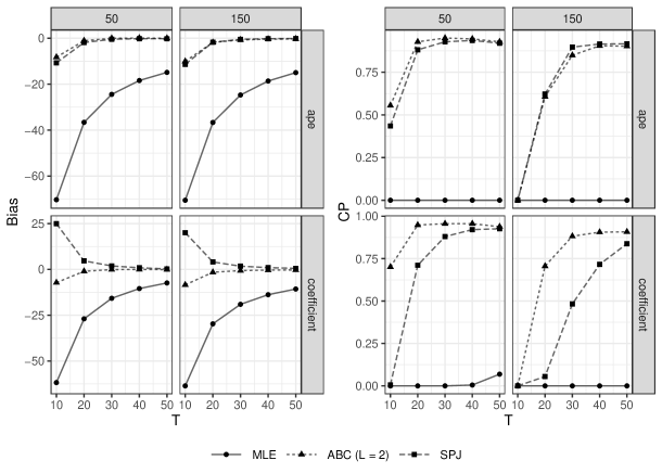
Figure 2: Dynamic: Three-way Fixed Effects — Predetermined Regressor

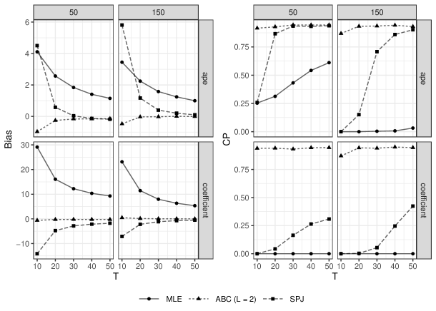
Figure 3: Dynamic: Three-way Fixed Effects — Exogenous Regressor

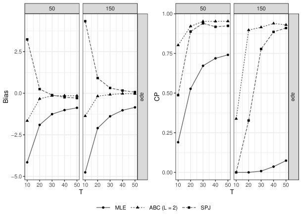
Figure 4: Dynamic: Three-way Fixed Effects — Exogenous Regressor (Long-Run)

We start by considering the different estimators for the structural parameters summarized in Figures 3 and 3. For both kinds of regressors, MLE exhibits a severe bias that decreases with increasing $T$. However, even with $N=150$ and $T=50$, the estimator shows a distortion of 11 percent in the case of the predetermined regressor and 5 percent in the case of the exogenous regressor. We also find that the inference is not valid, since the CPs are zero or close to zero. The bias corrections bring a substantial improvement. First, they reduce the bias considerably. For example, the MLE estimator of the predetermined regressor shows a distortion of 64 percent for $T=10$ and $N=150$. ABC reduces the bias to 8 percent and SPJ to 20 percent. In the case of the exogenous regressor, MLE exhibits a bias of 23 percent, whereas ABC has a bias of 1 percent and SPJ of 7 percent. Irrespective of the type of the regressor, both bias-corrected estimators also converge quickly to the true parameter value with growing $T$. Second, the bias corrections improve the CPs. For the exogenous regressor the CPs of ABC are close to the desired level of 95 percent for all $T$, whereas SPJ remains far away from 95 percent even at $T=50$. In the case of the predetermined regressor, the CPs of both corrections approach the nominal level when $T$ rises. This happens faster for ABC.

We proceed with the APEs, where we distinguish between direct and long-run APEs. We first look at the direct APEs in Figures 3 and 3. Overall, we obtain similar findings as for the structural parameters. MLE is distorted over all settings, but the bias decreases as $T$ increases. The distortion is especially severe in the case of the the predetermined regressor, where it ranges from roughly $70$ percent for the settings with $T=10$ to $15$ percent for $T=50$. In contrast, the bias of the MLE for the exogenous regressor ranges from roughly $4$ percent ($T=10$) to $1$ percent ($T=50$). The bias corrections bring a substantial reduction in both cases. Whereas ABC shows only a small distortion of less than $1$ percent in the case of the exogenous regressor at $T=10$, SPJ is even more heavily distorted than MLE. However, with increasing $T$, both SPJ and ABC quickly converge to the true APE. Looking at inference, unlike ABC, SPJ needs a sufficiently large number of time periods to get its CPs close to 95 percent. For the predetermined regressor, these convergence processes last longer than for the exogenous regressor. In contrast, the coverage probabilities of the MLE are always far below the desired nominal level. This is especially noteworthy for the exogenous regressor with $T\geq 40$, where the bias of MLE appears to be negligibly small for practical work. However, the bias of the MLE is still large compared to the standard error. This becomes evident, when looking at the Bias/SE ratio in Tables A6 – A6, which is much higher for MLE than for the bias corrected estimators. Turning to the results of the long-run APEs reported in Figure 4, we note that the results are qualitatively similar to the results of the direct APE of the exogenous regressor. As $T$ increases, both bias corrections quickly bring the bias towards zero and the coverage probabilities quickly reach the nominal level. Again, the convergence of ABC is faster and inference of MLE remains invalid despite small biases in settings with larger $T$.

Overall, our three-way fixed effects simulation results confirm the conjecture of [25] about the general form of the bias and lend support to our bias corrections. First, we find that the bias corrections indeed substantially mitigate the bias. Second, as already found in other studies, analytical bias corrections outperform split-panel jackknife bias corrections (see among others [24], and [15]). For samples with shorter time horizons, ABC is often less distorted and its dispersion is generally lower. This is also reflected by better CPs. Generally, in the three-way fixed effects setting, a sufficiently large number of time periods appears to be crucial to obtain reliable results for the bias-corrected estimators. As a main takeaway, our simulation results suggest that estimates based on MLE should be treated with great caution, because even in situations where we expect small biases, the inference may be invalid.

5 Determinants of the Extensive Margin of Trade

Having described the estimation and bias correction procedures, we now turn to the estimation of the determinants of the extensive margin of international trade outlined in Section 2.

Recall equation (3) that relates the incidence of non-zero aggregate trade flows to exporter-time and importer-time specific characteristics, trade in the previous period, time-invariant unobservable trade barriers and bilateral trade policy variables:

$$y_{ijt}=\begin{cases}1\quad\text{if}\quad\kappa+\lambda_{it}+\psi_{jt}+\beta_{y}y_{ij(t-1)}+\mathbf{z}_{ijt}^{\prime}\mbox{\boldmath${\beta}$}_{z}+\mu_{ij}\geq\zeta_{ijt},\\ 0\quad\text{else}\,.\end{cases}$$

This yields the following dynamic three-way fixed effects probit model:

$$\Pr(y_{ijt}=1|y_{ij(t-1)},\mathbf{z}_{ijt},\lambda_{it},\psi_{jt},\mu_{ij}) =F\left(\beta_{y}y_{ij(t-1)}+\mathbf{z}_{ijt}^{\prime}\mbox{\boldmath${\beta}$}_{z}+\lambda_{it}+\psi_{jt}+\mu_{ij}\right)\,,$$ (13)

$y_{ij(t-1)}$ is the lagged dependent variable, $\mathbf{z}$ is a vector of observable bilateral variables, and $\beta_{y}$ and $\beta_{z}$ are the corresponding parameters. We largely follow [35] and the wider literature on the determinants of the intensive margin of trade [32, compare] in the choice of these variables: distance, a common land border, the same origin of the legal system, common language, previous colonial ties, a joint currency, an existing free trade agreement, or joint membership in the WTO/GATT. The effect of all time-invariant variables will only be identified in specifications in which we omit the bilateral fixed effects.

For data, we turn to the updated Gravity dataset provided by CEPII [13], which encompasses annual information on bilateral trade flows and these variables of interest for 198 countries from 1948 – 2019. As only non-zero flows are reported in the data, we construct zeros analogous to [33]: Whenever an exporter reports at least one non-zero flow and an importer reports at least one non-zero flow, their bilateral flow — if not non-zero already — is coded as zero. This procedure results in an unbalanced data set with 1,652,296 observations.

Out of the 38,912 country pairs included in our analysis, 9,984 never switch their trading status, 4,609 switch a single time, and the average (median) number of switches is 3.9 (3), ranging up to 29 for trade from Benin to Sweden and 32 from Barbados to Bolivia.

5.1 Main Results

Before turning to the regression results, we repeat the descriptive analysis about the persistence of the bilateral trade flows from Section 1, now considering the transition probabilities into export from period $t-1$ to $t$ for the time horizon from 1948 – 2019. Table 3 confirms the high level of persistence: 89.7 percent of the country pairs which did not trade in the previous year did not trade in the following year and 91.5 percent of the pairs which did trade in the previous year continued to trade in the following year. Thus, the probability to export in period $t$ is 81.2 percentage points higher for those country pairs that already engaged in trade in period $t-1$ compared to those that did not. However, Table 3 does not reveal any information about the kind of persistence. In the following analysis we will investigate the importance of using dynamic model specifications which allow us to disentangle the observed persistence into two sources: (i) true state dependence and (ii) observed and unobserved heterogeneity.

Table 3: Transition Probabilities (1948 – 2019)

	$y_{ijt}=0$	$y_{ijt}=1$
$y_{ij(t-1)}=0$	89.7 %	10.3 %
$y_{ij(t-1)}=1$	8.6 %	91.5 %

In the following analysis we only consider analytically bias-corrected estimates, mainly for two reasons: (1) the simulation results demonstrate that ABC performs much better than SPJ; (2) SPJ requires the additional homogeneity assumption, which is likely to be violated in our application. Progressing economic integration over time — be it through an increasing number of WTO/GATT memberships or through bilateral and multilateral integration in the form of currency unions and free trade agreements — is at odds with the required stationary pattern.

Table 4 reports average partial effects of several static and dynamic fixed effects probit specifications. Bias-corrected estimates and their corresponding standard errors are printed in bold. For comparison, the uncorrected estimates are also shown. In column (1) we first mimic the static specification estimated by [35]. Their specification includes exporter, importer, and time fixed effects. All average partial effects have the expected sign, indicating a negative impact of distance on the probability to trade, while having a common border, the same origin of the legal system, a shared language, or a joint colonial history are all estimated to have a positive impact. Also note the strong and highly significant impact of a common currency, free trade agreement or joint membership of the WTO/GATT. Ceteris paribus, each is estimated to increase the probability of non-zero flows by between 5.2 and 7.1 percentage points.

Table 4: Probit Estimation: Average partial effects

	Dependent variable: $y_{ijt}$
	(1)	(2)	(3)		(4)	(5)
			direct	long-run		direct	long-run
$y_{ij(t-1)}$	-	-	0.394***	-	-	0.187***	-
	(-)	(-)	(0.001)	(-)	(-)	(0.001)	(-)
	-	-	0.393***	-	-	0.148***	-
	(-)	(-)	(0.001)	(-)	(-)	(0.001)	(-)
log(Distance)	-	-0.141***	-0.066***	-0.141***	-	-	-
	(-)	(0.000)	(0.000)	(0.001)	(-)	(-)	(-)
	-0.141***	-0.141***	-0.066***	-0.141***	-	-	-
	(0.001)	(0.000)	(0.000)	(0.001)	(-)	(-)	(-)
Land border	-	0.024***	0.010***	0.021***	-	-	-
	(-)	(0.004)	(0.002)	(0.004)	(-)	(-)	(-)
	0.034***	0.025***	0.011***	0.023***	-	-	-
	(0.004)	(0.004)	(0.002)	(0.004)	(-)	(-)	(-)
Legal	-	0.006***	0.003***	0.006***	-	-	-
	(-)	(0.001)	(0.001)	(0.001)	(-)	(-)	(-)
	0.005***	0.006***	0.003***	0.006***	-	-	-
	(0.001)	(0.001)	(0.001)	(0.001)	(-)	(-)	(-)
Language	-	0.071***	0.034***	0.073***	-	-	-
	(-)	(0.001)	(0.001)	(0.002)	(-)	(-)	(-)
	0.074***	0.072***	0.034***	0.073***	-	-	-
	(0.001)	(0.001)	(0.001)	(0.002)	(-)	(-)	(-)
Colonial ties	-	0.051***	0.023***	0.049***	-	-	-
	(-)	(0.001)	(0.001)	(0.002)	(-)	(-)	(-)
	0.053***	0.051***	0.023***	0.048***	-	-	-
	(0.001)	(0.001)	(0.001)	(0.002)	(-)	(-)	(-)
Currency union	-	0.097***	0.045***	0.095***	0.034***	0.022***	0.034***
	(-)	(0.003)	(0.002)	(0.004)	(0.004)	(0.004)	(0.006)
	0.071***	0.097***	0.046***	0.096***	0.034***	0.023***	0.034***
	(0.003)	(0.003)	(0.002)	(0.004)	(0.004)	(0.004)	(0.005)
FTA	-	0.054***	0.025***	0.054***	0.012***	0.008***	0.012***
	(-)	(0.001)	(0.001)	(0.002)	(0.002)	(0.002)	(0.002)
	0.053***	0.054***	0.025***	0.052***	0.011***	0.007***	0.011***
	(0.001)	(0.001)	(0.001)	(0.002)	(0.002)	(0.002)	(0.002)
WTO / GATT	-	0.034***	0.016***	0.034***	0.013***	0.008***	0.013***
	(-)	(0.001)	(0.001)	(0.002)	(0.002)	(0.001)	(0.002)
	0.052***	0.034***	0.016***	0.034***	0.012***	0.009***	0.013***
	(0.001)	(0.001)	(0.001)	(0.002)	(0.002)	(0.001)	(0.002)
Fixed effects	$i,j,t$	$it,jt$	$it,jt$		$it,jt,ij$	$it,jt,ij$
Sample size	1652296	1652296	1613354		1652296	1613354
Deviance	11.65$\times$104	9.90$\times$104	7.17$\times$104		6.50$\times$104	5.76$\times$104
Notes: Column (1) uncorrected average partial effects, columns (2) - (5) bias-corrected average partial effects (bold font) and uncorrected average partial effects (normal font). Columns (4) and (5) bias-corrected with $L=2$. Standard errors in parenthesis. ${}^{***}p<0.01$, ${}^{**}p<0.05$, ${}^{*}p<0.1$

Column (2) introduces a stricter set of fixed effects, namely at the exporter-time and importer-time level. This specification can be considered a theory-consistent estimation of the model by HMR, and of our model if entry costs are zero and other bilateral trade cost determinants are fully observable. The average partial effects are qualitatively the same and quantitatively similar for most variables to those in column (1). However, e.g. the estimated effects of contiguity and joint WTO/GATT membership are reduced by more than a third, while the estimated effect of sharing a common currency increases by 2.6 percentage points or 37 percent.

Specification (3) keeps the same fixed effects, but adds a lagged dependent variable and thus controls for one type of persistence. Assuming no unobservable bilateral heterogeneity, this specification correctly estimates the model set up in Section 2. As the partial effects of static and dynamic models are not directly comparable due to the feedbacks involved in the latter, we show two types of average partial effects for our dynamic specifications: the usual direct effects and the long-run effects described in Section 3. The first result to note for the third specification is the highly significant average partial effect for the lagged dependent variable, which reflects the strong impact of previous non-zero trade flows on current ones. Ceteris paribus, the average partial effect shows a 39.4 percentage points higher probability of non-zero trade, given the two countries were also engaged in trade in the previous year. This implies that 48.5 percent of the observed persistence are attributed to true state dependence in this first dynamic specification. In terms of our model, this suggests a vast effect of market entry costs on the aggregate extensive margin. The second observation is that direct APEs are about 50 percent smaller than in column (2) across the board. However, once dynamic adjustments are taken into account, the average partial effects resulting from specifications (2) and (3) become very similar, suggesting that accounting for the market entry dynamics mainly matters for getting the timing of trade policy effects right, rather than for the overall magnitude of the effects.

Specification (4) takes one step back and one forward. While not including the lagged dependent variable in the estimation, it introduces a bilateral fixed effect that controls for a second type of persistence — bilateral unobserved heterogeneity. This also follows the important insight by [4], who show that controlling for unobserved bilateral heterogeneity produces a considerably different estimated impact of free trade agreements, among other variables, on the intensive margin of trade. While now an identification of many of the variables of interest is no longer possible because of their time invariance, this specification reveals a much reduced estimated impact of the time-varying variables. The impact of a common currency on the probability of exporting is reduced to 3.4 percentage points, while those of a common free trade agreement and WTO/GATT are decreased to 1.2 and 1.3 percentage points, respectively. These results highlight the importance of controlling for unobserved country pair heterogeneity to avoid endogeneity problems associated with trade policy variables.

Finally, in the last two columns we present the results from our preferred specification (5), which implements equation (13). The estimation again includes the “full set” of fixed effects, i.e. exporter-time, importer-time and bilateral fixed effects, now combined with the lagged dependent variable, and therefore controls for both kinds of persistence simultaneously. Again, the average partial effect on the lagged dependent variable is highly significant. It now entails a partial effect of about 18.7 percentage points, i.e. roughly 23 percent of the observed persistence can be attributed to true state dependence and 77 percent to other observed factors and unobserved heterogeneity. Failure to account for unobserved heterogeneity in specification (3) hence overestimated the importance of the lagged dependent variable (corresponding to entry costs in our model) roughly by a factor of two and therefore mislabelled a substantial part of spurious as true state dependence. Considering the effects of the time-varying trade policy variables, small but statistically significant direct average partial effects in column (5) are estimated for a common currency at 2.2 percentage points and for both joint FTA and WTO memberships at 0.8 percentage points. Just as in the comparison between specifications (2) and (3), the average partial effects again become very similar when the static effects are compared to the long-run effects in the dynamic specification.

When comparing bias-corrected and uncorrected average partial effects throughout Table 4, it is noticeable that both differ only slightly for the exogenous regressors within the different specifications. The most significant impact is observed on the average partial effect for the predetermined variable, which in specification (5) differs by more than 26 percent. These results are in line with the theoretical properties of the estimators and the findings of our simulation study. Despite the small biases for the exogenous variables, a bias correction is still necessary for our three-way fixed effects specifications because the biases are not negligible relative to the standard errors and thus inference of the uncorrected estimator is invalid. Note that for applications with a shorter time horizon, the biases will be more evident.

5.2 Predictive Analysis

After we have seen that the presented innovations matter significantly for the estimation of extensive margin determinants, we now consider the predictive performance of the different specifications discussed above. As an additional benchmark, we also look at a naive — purely descriptive — approach that predicts export decisions in period $t$ solely based on the export decision in period $t-1$. For the resulting altogether six options, we evaluate the predictive power using the following measures: the total share of correctly predicted export decisions (accuracy), the share of correctly predicted decisions conditional on not exporting (true negative rate), and the share of correctly predicted decisions conditional on exporting (true positive rate). As becomes clear in Table 5, the naive approach already works very well for predictive purposes. Close to 90 percent of the exporting decisions in period $t$ are correctly predicted by simply reproducing exporting decisions from $t-1$, irrespective of the measure we are considering. As it turns out, both the static model with $i$, $j$, and $t$ fixed effects (specification (1)) and the static model with $it$ and $jt$ fixed effects (specification (2)) produce poorer predictions than the naive approach — particularly clearly so by about six percentage points in the former case. However, this changes once persistence is explicitly taken into account in specifications (3) to (5). All of them at least slightly improve the predictions of the naive approach. Whether persistence is incorporated only via the lagged dependent variable or via pair fixed effects turns out to yield very similar predictive quality. Combining both in our preferred specification — the dynamic three-way fixed effects models — yields the highest predictive power. We are able to correctly predict 92.6 percent of the export decisions, 91.4 percent of the decisions conditional on not exporting, and 93.5 percent of the decisions conditional on exporting, implying an improvement compared to the naive approach by around 2 percentage points. All in all, the predictive analysis underlines the importance of controlling for true state dependence and unobserved bilateral factors simultaneously.

Table 5: Predictive Analysis

	Naive	(1)	(2)	(3)	(4)	(5)
Accuracy	90.6 %	84.5 %	86.9 %	91.4 %	91.5 %	92.6 %
True negative rate	91.5 %	85.6 %	87.7 %	92.3 %	92.5 %	93.5 %
True positive rate	89.7 %	83.3 %	86.0 %	90.4 %	90.6 %	91.7 %
Notes: Column (1) uncorrected probit model, columns (2) – (5) bias-corrected probit model.

5.3 Robustness Checks

Table 6: Logit Estimation: Average partial effects

	Dependent variable: $y_{ijt}$
	(1)	(2)	(3)		(4)	(5)
			direct	long-run		direct	long-run
$y_{ij(t-1)}$	-	-	0.373***	-	-	0.169***	-
	(-)	(-)	(0.001)	(-)	(-)	(0.001)	(-)
	-	-	0.375***	-	-	0.136***	-
	(-)	(-)	(0.001)	(-)	(-)	(0.001)	(-)
log(Distance)	-	-0.144***	-0.067***	-0.142***	-	-	-
	(-)	(0.000)	(0.000)	(0.001)	(-)	(-)	(-)
	-0.144***	-0.144***	-0.067***	-0.142***	-	-	-
	(0.000)	(0.000)	(0.000)	(0.001)	(-)	(-)	(-)
Land border	-	0.053***	0.011***	0.022***	-	-	-
	(-)	(0.003)	(0.002)	(0.004)	(-)	(-)	(-)
	0.057***	0.054***	0.012***	0.025***	-	-	-
	(0.003)	(0.003)	(0.002)	(0.004)	(-)	(-)	(-)
Legal	-	0.007***	0.003***	0.006***	-	-	-
	(-)	(0.001)	(0.001)	(0.001)	(-)	(-)	(-)
	0.007***	0.007***	0.003***	0.006***	-	-	-
	(0.001)	(0.001)	(0.001)	(0.001)	(-)	(-)	(-)
Language	-	0.069***	0.035***	0.073***	-	-	-
	(-)	(0.001)	(0.001)	(0.002)	(-)	(-)	(-)
	0.072***	0.070***	0.035***	0.073***	-	-	-
	(0.001)	(0.001)	(0.001)	(0.002)	(-)	(-)	(-)
Colonial ties	-	0.052***	0.024***	0.049***	-	-	-
	(-)	(0.001)	(0.001)	(0.002)	(-)	(-)	(-)
	0.055***	0.052***	0.023***	0.049***	-	-	-
	(0.001)	(0.001)	(0.001)	(0.002)	(-)	(-)	(-)
Currency union		0.097***	0.046***	0.096***	0.034***	0.022***	0.035***
	(-)	(0.003)	(0.002)	(0.004)	(0.004)	(0.004)	(0.006)
	0.071***	0.098***	0.047***	0.097***	0.034***	0.024***	0.035***
	(0.002)	(0.003)	(0.002)	(0.004)	(0.004)	(0.004)	(0.006)
FTA	-	0.056***	0.026***	0.054***	0.015***	0.008***	0.013***
	(-)	(0.001)	(0.001)	(0.002)	(0.002)	(0.002)	(0.002)
	0.054***	0.056***	0.025***	0.053***	0.014***	0.008***	0.012***
	(0.001)	(0.001)	(0.001)	(0.002)	(0.002)	(0.002)	(0.002)
WTO/GATT	-	0.028***	0.016***	0.034***	0.012***	0.009***	0.014***
	(-)	(0.001)	(0.001)	(0.002)	(0.002)	(0.001)	(0.002)
	0.049***	0.028***	0.016***	0.034***	0.012***	0.009***	0.013***
	(0.001)	(0.001)	(0.001)	(0.002)	(0.002)	(0.002)	(0.002)
Fixed effects	$i,j,t$	$it,jt$	$it,jt$		$it,jt,ij$	$it,jt,ij$
Sample size	1652296	1652296	1613354		1652296	1613354
Deviance	11.57$\times$105	9.81$\times$105	7.20$\times$105		6.44$\times$105	5.75$\times$105
Notes: Column (1) uncorrected average partial effects, columns (2) - (5) bias-corrected average partial effects (bold font) and uncorrected average partial effects (normal font). Columns (4) and (5) bias-corrected with $L=2$. Standard errors in parenthesis. ${}^{***}p<0.01$, ${}^{**}p<0.05$, ${}^{*}p<0.1$

We next consider two robustness checks for our main results from Section 5.1. First, while our preferred estimation of the extensive margin of trade with a dynamic three-way fixed effects binary choice estimator follows from the stylized facts and our theoretical model, the decision on which binary choice estimator to use hinges on the distributional assumption for the error term (and hence for the demand shock in our model). We followed [19] and assumed log-normal shocks, leading us to using a probit for our main estimations. We now consider log-logistic shocks and the resulting logit estimator instead. Table 6 displays the results for the same specifications as in Table 4, but estimated using a logit. Reassuringly, the average partial effects are very similar to the probit case for all variables in all specifications. Introducing the different innovations step-by-step changes the estimated effects in the same way as for the probit. The insights discussed above therefore do not hinge on the specific distributional assumption made in the parametrization of the probability of success.

Second, in the estimation of our preferred specification (5) we have discretionary power in one dimension for the exact form of bias correction used. Specifically, the bandwidth parameter $L$ used to estimate the spectral densities has to be chosen. We therefore follow the recommendation by [24] and investigate the sensitivity of the results with respect to $L$. Table 7 depicts the direct and long-run average partial effects obtained with the bias-corrected dynamic three-way fixed effects probit estimator for $L\in\{1,2,3,4\}$. Again, our results turn out to be very robust. There only appears to be a slight upward trend in the estimated true state dependence for larger $L$.

Table 7: Probit Estimation with Different Bandwidths: Bias-Corrected Average Partial Effects

	Dependent variable: $y_{ijt}$
	$L=1$		$L=2$		$L=3$		$L=4$
	direct	long-run	direct	long-run	direct	long-run	direct	long-run
$y_{ij(t-1)}$	0.181***	-	0.187***	-	0.191***	-	0.192***	-
	(0.001)	(-)	(0.001)	(-)	(0.001)	(-)	(0.001)	(-)
Currency union	0.022***	0.034***	0.022***	0.034***	0.022***	0.034***	0.022***	0.035***
	(0.004)	(0.006)	(0.004)	(0.006)	(0.004)	(0.006)	(0.004)	(0.006)
FTA	0.008***	0.012***	0.008***	0.012***	0.008***	0.012***	0.008***	0.012***
	(0.002)	(0.002)	(0.002)	(0.002)	(0.002)	(0.002)	(0.002)	(0.002)
WTO/GATT	0.008***	0.013***	0.008***	0.013***	0.009***	0.014***	0.009***	0.014***
	(0.001)	(0.002)	(0.001)	(0.002)	(0.001)	(0.002)	(0.001)	(0.002)
Notes: All columns include Origin $\times$ Year, Destination $\times$ Year and Origin $\times$ Destination fixed effects. Standard errors in parenthesis. ${}^{***}p<0.01$, ${}^{**}p<0.05$, ${}^{*}p<0.1$

6 Conclusion

In this paper we reexamine the determinants of the extensive margin of international trade. We set up a model that exhibits a dynamic component and allows for time-invariant unobserved bilateral trade cost factors, generating persistence — a feature in the data that has so far been given little attention. For the estimation of our model, we propose new bias-corrected fixed effects binary choice estimators to account for the incidental parameters problem and to deal with weakly exogenous regressors. Finally, we show that our estimates of the determinants of the extensive margin of trade differ significantly from previous ones. This highlights the importance of true state dependence and unobserved heterogeneity and therefore strongly supports the use of our bias-corrected dynamic fixed effects estimator.

The extensive margin of trade obviously extends beyond the aggregate level, warranting further research at lower levels of aggregation, in particular in the context of firms. While our model’s prediction and its empirical specification rely on some abstractions, it provides a very tractable and flexible framework that can be estimated with recently established estimation procedures, when combined with the bias correction technique we introduce.

A further natural extension for future research would be to define the extensive margin as the number of exporting sectors leading to a fractional instead of a binary outcome [45, 3, as in]. Following the insights for such conditional moment models by [24], our split-panel jackknife estimator can be directly applied and the analytical bias correction has to only be slightly adjusted for the fractional outcome setting.

Online Appendix

Appendix A Stylized facts

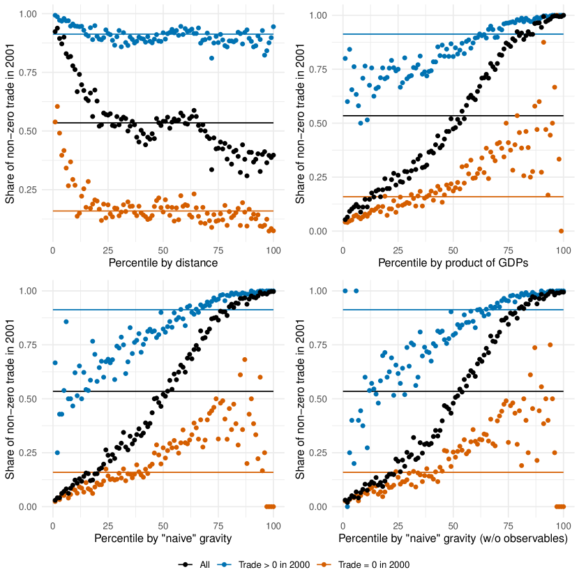
Figure A1: Determinants of the Extensive margin of Trade — Gravity and Persistence (2000–2001).

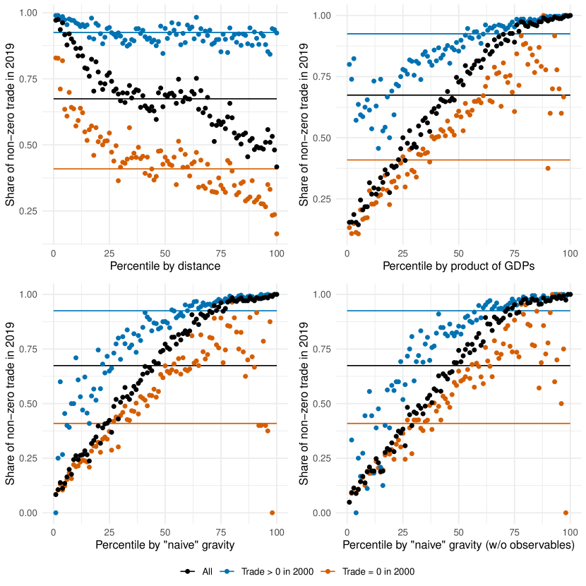
Figure A2: Determinants of the Extensive Margin of Trade — Gravity and Persistence (2000–2019).

Appendix B Econometric Details

B.1 Computational Details

In this section we briefly demonstrate how the method of alternating projections (MAP) works in the context of logit and probit models with a two- or three-way error component, and how it can be efficiently embedded into a standard Newton-Raphson optimization routine [46, see].

First, note that $\operatorname{\mathbb{M}}\mathbf{v}$ is essentially a weighted within transformation, where $\mathbf{v}$ is an arbitrary $n\times 1$ vector, and $\operatorname{\mathbb{M}}=\mathbf{I}_{n}-\operatorname{\mathbb{P}}=\mathbf{I}_{n}-\mathbf{D}(\mathbf{D}^{\prime}\bm{\Omega}\mathbf{D})^{-1}\mathbf{D}^{\prime}\bm{\Omega}$. The computation of $\operatorname{\mathbb{M}}$ is problematic even in moderately large data sets, and since $\operatorname{\mathbb{M}}$ is non-sparse, there is also no general scalar expression to compute $\operatorname{\mathbb{M}}\mathbf{v}$. Thus [46] proposes to calculate $\operatorname{\mathbb{M}}\mathbf{v}$ using a simple iterative approach based on the MAP tracing back to [47] and [31]. Let $\mathbf{D}_{k}$, denote the dummy variables corresponding to the $k$-th group, $k\in\{1,2,3\}$. Further, let $\operatorname{\mathbb{M}}_{\mathbf{D}_{k}}\mathbf{v}$, with $\operatorname{\mathbb{M}}_{\mathbf{D}_{k}}=\mathbf{I}_{n}-\mathbf{D}_{k}(\mathbf{D}_{k}^{\prime}\bm{\Omega}\mathbf{D}_{k})^{-1}\mathbf{D}_{k}^{\prime}\bm{\Omega}$. The corresponding scalar expressions of $\operatorname{\mathbb{M}}_{\mathbf{D}_{k}}\mathbf{v}$ are summarized in Table (A1).

Table A1: Scalar Transformations

group	$\operatorname{\mathbb{M}}_{\mathbf{D}_{k}}\mathbf{v}$
importer-time ($k=1$)	$\mathbf{v}_{ijt}-\frac{\sum_{j=1}^{J}\omega_{ijt}v_{ijt}}{\sum_{j=1}^{J}\omega_{ijt}}$
exporter-time ($k=2$)	$\mathbf{v}_{ijt}-\frac{\sum_{i=1}^{I}\omega_{ijt}v_{ijt}}{\sum_{i=1}^{I}\omega_{ijt}}$
dyadic ($k=3$)	$\mathbf{v}_{ijt}-\frac{\sum_{t=1}^{T}\omega_{ijt}v_{ijt}}{\sum_{t=1}^{T}\omega_{ijt}}$

The MAP can be summarized by algorithm 1, where $K=2$ in the case of two-way fixed effects and $K=3$ in the case of three-way fixed effects. Thus, the MAP only requires to repeatedly apply weighted one-way within transformations [46, see]. The entire optimization routine is sketched by algorithm 2.

Algorithm 1 MAP: Neumann-Halperin

1:Initialize $\operatorname{\mathbb{M}}\mathbf{v}=\mathbf{v}$.

2:repeat

3:     for $k=1,\dots,K$ do

4:         Compute $\operatorname{\mathbb{M}}_{\mathbf{D}_{k}}\operatorname{\mathbb{M}}\mathbf{v}$ and update $\operatorname{\mathbb{M}}\mathbf{v}$ such that $\operatorname{\mathbb{M}}\mathbf{v}=\operatorname{\mathbb{M}}_{\mathbf{D}_{k}}\operatorname{\mathbb{M}}\mathbf{v}$      

5:until convergence.

Algorithm 2 Efficient Newton-Raphson using the MAP

1:Initialize $\bm{\beta}^{0}$, $\bm{\eta}^{0}$, and $r=0$.

2:repeat

3:     Set $r=r+1$.

4:     Given $\hat{\bm{\eta}}^{r-1}$ compute $\hat{\bm{\nu}}$ and $\widehat{\bm{\Omega}}$.

5:     Given $\hat{\bm{\nu}}$ and $\widehat{\bm{\Omega}}$ compute $\widehat{\operatorname{\mathbb{M}}}\hat{\bm{\nu}}$ and $\widehat{\operatorname{\mathbb{M}}}\mathbf{X}$ using the MAP

6:     Compute $\bm{\beta}^{r}-\bm{\beta}^{r-1}=\left((\widehat{\operatorname{\mathbb{M}}}\mathbf{X})^{\prime}\widehat{\bm{\Omega}}(\widehat{\operatorname{\mathbb{M}}}\mathbf{X})\right)^{-1}(\widehat{\operatorname{\mathbb{M}}}\mathbf{X})^{\prime}\widehat{\bm{\Omega}}(\widehat{\operatorname{\mathbb{M}}}\hat{\bm{\nu}})$

7:     Compute $\hat{\bm{\eta}}^{r}=\hat{\bm{\eta}}^{r-1}+\hat{\bm{\nu}}-\widehat{\operatorname{\mathbb{M}}}\hat{{\bm{\nu}}}+\widehat{\operatorname{\mathbb{M}}}\mathbf{X}(\bm{\beta}^{r}-\bm{\beta}^{r-1})$

8:until convergence.

B.2 Neyman-Scott Variance Example

In this section we study two variants of the classical [38] variance example to support the form of the bias terms, and to illustrate the functionality of the bias corrections. To the best of our knowledge, the variance example of [38] has not been investigated for our specific error components. We start with the more general three-way fixed effects case, which nests the two-way error structure. To make the dependence of the estimators on the sample size explicit, we use the subscript $I,J,T$ throughout the Appendix.

B.2.1 Three-way Fixed Effects

Let $i=1,\dots,I$, $j=1,\dots,J$ and $t=1,\dots,T$. Consider the following linear three-way fixed effects model

$$y_{ijt}=\mathbf{x}_{ijt}^{\prime}\bm{\beta}+\lambda_{it}+\psi_{jt}+\mu_{ij}+u_{ijt}\;.$$ (A1)

According to [5], the appropriate within transformation corresponding to equation (A1) is given by

$$z_{ijt}-\bar{z}_{ij\cdot}-\bar{z}_{\cdot jt}-\bar{z}_{i\cdot t}+\bar{z}_{\cdot\cdot t}+\bar{z}_{\cdot j\cdot}+\bar{z}_{i\cdot\cdot}-\bar{z}_{\cdot\cdot\cdot}\;,$$

where $\bar{z}_{ij\cdot}=\frac{1}{T}\sum_{t=1}^{T}z_{ijt}$, $\bar{z}_{\cdot jt}=\frac{1}{I}\sum_{i=1}^{I}z_{ijt}$, $\bar{z}_{i\cdot t}=\frac{1}{J}\sum_{j=1}^{J}z_{ijt}$, $\bar{z}_{\cdot\cdot t}=\frac{1}{IJ}\sum_{i=1}^{I}\sum_{j=1}^{J}z_{ijt}$, $\bar{z}_{\cdot j\cdot}=\frac{1}{IT}\sum_{i=1}^{I}\sum_{t=1}^{T}z_{ijt}$, $\bar{z}_{i\cdot\cdot}=\frac{1}{JT}\sum_{j=1}^{J}\sum_{t=1}^{T}z_{ijt}$, and $\bar{z}_{\cdot\cdot\cdot}=\frac{1}{IJT}\sum_{i=1}^{I}\sum_{j=1}^{J}\sum_{t=1}^{T}z_{ijt}$.

This result is helpful to study the following variant of the [38] variance example

$$y_{ijt}|\bm{\lambda},\bm{\psi},\bm{\mu}\sim\mathcal{N}(\lambda_{it}+\psi_{jt}+\mu_{ij},\beta)\;,$$

where we can now easily form the uncorrected variance estimator

$$\hat{\beta}_{I,J,T}=\frac{1}{IJT}\sum_{i=1}^{I}\sum_{j=1}^{J}\sum_{t=1}^{T}(y_{ijt}-\bar{y}_{ij\cdot}-\bar{y}_{\cdot jt}-\bar{y}_{i\cdot t}+\bar{y}_{\cdot\cdot t}+\bar{y}_{\cdot j\cdot}+\bar{y}_{i\cdot\cdot}-\bar{y}_{\cdot\cdot\cdot})^{2}$$ (A2)

and the (degrees-of-freedom)-corrected counterpart

$$\hat{\beta}_{I,J,T}^{cor}=\frac{IJT}{(I-1)(J-1)(T-1)}\hat{\beta}_{I,J,T}\;.$$

Taking the expectation of (A2) (conditional on the fixed effects) yields

$$\bar{\beta}_{I,J,T}=\operatorname{\mathbb{E}}_{\alpha}[\hat{\beta}_{I,J,T}] =\beta^{0}\left(\frac{(I-1)(J-1)(T-1)}{IJT}\right)$$ (A3)

$$=\beta^{0}\left(1-\frac{1}{I}-\frac{1}{J}-\frac{1}{T}+\frac{1}{IT}+\frac{1}{JT}+\frac{1}{IJ}-\frac{1}{IJT}\right)\;,$$

where $\beta^{0}$ is the true variance parameter. Thus, the three leading bias terms, which drive the main part of the asymptotic bias, are $\overline{\mathbf{B}}_{1,\infty}^{\beta}=-\beta^{0}$, $\overline{\mathbf{B}}_{2,\infty}^{\beta}=-\beta^{0}$, and $\overline{\mathbf{B}}_{3,\infty}^{\beta}=-\beta^{0}$.

Analytical Bias Correction

Using equation (A3), we can form the analytically bias-corrected estimator

$$\tilde{\beta}_{I,J,T}^{a} =\hat{\beta}_{I,J,T}-\frac{\widehat{\mathbf{B}}^{\beta}_{1,I,J,T}}{I}-\frac{\widehat{\mathbf{B}}^{\beta}_{2,I,J,T}}{J}-\frac{\widehat{\mathbf{B}}^{\beta}_{3,I,J,T}}{T}\;,$$ (A4)

where we set $\widehat{\mathbf{B}}^{\beta}_{1,I,J,T}=-\hat{\beta}_{I,J,T}$, $\widehat{\mathbf{B}}^{\beta}_{2,I,J,T}=-\hat{\beta}_{I,J,T}$, and $\widehat{\mathbf{B}}^{\beta}_{3,I,J,T}=-\hat{\beta}_{I,J,T}$ to reduce the order of the bias in equation (A3) at costs of introducing higher order terms (see equation (A6)). Thus, we can rewrite the analytically bias-corrected estimator (A4)

$$\tilde{\beta}_{I,J,T}^{a}=\hat{\beta}_{I,J,T}\left(1+\frac{1}{I}+\frac{1}{J}+\frac{1}{T}\right)\;.$$ (A5)

Taking the expectation of (A5) yields

$$\bar{\beta}_{I,J,T}^{a}=\operatorname{\mathbb{E}}_{\alpha}[\tilde{\beta}_{I,J,T}^{a}] =\beta^{0}\left(1-\frac{1}{I}-\frac{1}{J}-\frac{1}{T}+\frac{1}{IT}+\frac{1}{JT}+\frac{1}{IJ}-\frac{1}{IJT}\right)\left(1+\frac{1}{I}+\frac{1}{J}+\frac{1}{T}\right)$$ (A6)

$$=\beta^{0}\left(1-\frac{1}{IT}-\frac{1}{JT}-\frac{1}{T^{2}}-\frac{3}{IJ}+\frac{1}{I^{3}}+\frac{1}{J^{3}}+\frac{4}{IJT}+\frac{1}{IT^{2}}+\frac{1}{JT^{2}}\right.$$

$$\qquad\qquad\left.-\frac{1}{I^{3}T}-\frac{1}{J^{3}T}-\frac{1}{IJT^{2}}\right)\;.$$

Split-Panel Jackknife

As an alternative to equation (A5) we can also form the following SPJ estimator

$$\hat{\beta}_{I,J,T}^{spj}=4\hat{\beta}_{I,J,T}-\hat{\beta}_{I/2,J,T}-\hat{\beta}_{I,J/2,T}-\hat{\beta}_{I,J,T/2}\;,$$

where $\hat{\beta}_{I/2,J,T}$ denotes the half panel estimator based on splitting the panel by exporters. This estimator also reduces the order of the bias in equation (A3) as we see from its expected value

$$\bar{\beta}_{I,J,T}^{spj}=E_{\phi}[\hat{\beta}_{I,J,T}^{spj}] =4\bar{\beta}_{I,J,T}-\bar{\beta}_{I/2,J,T}-\bar{\beta}_{I,J/2,T}-\bar{\beta}_{I,J,T/2}$$ (A7)

$$=\beta^{0}\left(1-\frac{1}{IT}-\frac{1}{JT}-\frac{1}{IJ}+\frac{2}{IJT}\right)\;.$$

Numerical Results

Table A2 shows numerical results for the uncorrected and the bias-corrected estimators in finite samples, where we assume symmetry, i.e. $I=J=N$. The results demonstrate that the bias corrections are effective in reducing the bias.

Table A2: Bias - Three-way Fixed Effects

N	T	$(\bar{\beta}_{I,J,T}-\beta^{0})/\beta^{0}$	$(\bar{\beta}_{I,J,T}^{a}-\beta^{0})/\beta^{0}$	$(\bar{\beta}_{I,J,T}^{spj}-\beta^{0})/\beta^{0}$
10	10	-0.271	-0.052	-0.028
25	10	-0.171	-0.021	-0.009
25	25	-0.115	-0.009	-0.005
50	10	-0.136	-0.015	-0.004
50	25	-0.078	-0.004	-0.002
50	50	-0.059	-0.002	-0.001

B.2.2 Two-way Fixed Effects

In the following we briefly review the example with two-way fixed effects

$$y_{ijt}|\bm{\lambda},\bm{\psi}\sim\mathcal{N}(\lambda_{it}+\psi_{jt},\beta)\;.$$

Since it is a subcase of three-way fixed effects example, all previous results simplify by dropping the terms that exhibit $T$.

The uncorrected variance estimator is

$$\hat{\beta}_{I,J,T}=\frac{1}{IJT}\sum_{i=1}^{I}\sum_{j=1}^{J}\sum_{t=1}^{T}(y_{ijt}-\bar{y}_{\cdot jt}-\bar{y}_{i\cdot t}+\bar{y}_{\cdot\cdot t})^{2}$$

and the (degrees-of-freedom)-corrected variance estimator is

$$\hat{\beta}_{I,J,T}^{cor}=\frac{IJ}{(I-1)(J-1)}\hat{\beta}_{I,J,T}\;.$$

Taking the expected value yields

$$\bar{\beta}_{I,J,T}=\operatorname{\mathbb{E}}_{\alpha}[\hat{\beta}_{I,J,T}] =\beta^{0}\left(\frac{(I-1)^{2}}{IJ}\right)$$ (A8)

$$=\beta^{0}\left(1-\frac{1}{I}-\frac{1}{J}+\frac{1}{IJ}\right)\;.$$

Analytical Bias Correction

Based on equation (A8) we can form the following analytically bias-corrected estimator

$$\tilde{\beta}_{I,J,T}^{a}=\hat{\beta}_{I,J,T}\left(1+\frac{1}{I}+\frac{1}{J}\right)\;,$$

which has the expected value

$$\bar{\beta}_{I,J,T}^{a}=\operatorname{\mathbb{E}}_{\alpha}[\tilde{\beta}_{I,J,T}^{a}]=\beta^{0}\left(1-\frac{3}{IJ}+\frac{1}{I^{3}}+\frac{1}{J^{3}}\right)\;.$$

Split-Panel Jackknife

A suitable split-panel jackknife estimator is

$$\hat{\beta}_{I,J,T}^{spj}=4\hat{\beta}_{I,J,T}-\hat{\beta}_{I/2,J,T}-\hat{\beta}_{I,J/2,T}\;,$$

which has the expected value

$$\bar{\beta}_{I,J,T}^{spj}=\operatorname{\mathbb{E}}_{\alpha}[\hat{\beta}_{I,J,T}^{spj}] =3\bar{\beta}_{I,J,T}-\bar{\beta}_{I/2,J,T}-\bar{\beta}_{I,J/2,T}$$

$$=\beta^{0}\left(1-\frac{1}{IJ}\right)\;.$$

Numerical Results

The numerical results in Table A3 demonstrate that the bias corrections work.

Table A3: Bias - Two-way Fixed Effects

N	$(\bar{\beta}_{I,J,T}-\beta^{0})/\beta^{0}$	$(\bar{\beta}_{I,J,T}^{a}-\beta^{0})/\beta^{0}$	$(\bar{\beta}_{I,J,T}^{spj}-\beta^{0})/\beta^{0}$
10	-0.190	-0.028	-0.010
25	-0.078	-0.005	-0.002
50	-0.040	-0.001	-0.000
100	-0.020	-0.000	-0.000

B.3 Asymptotic Bias Corrections

For the following expressions we draw on the results of [24], who have already derived the asymptotic distributions of the MLE estimators for structural parameters and APEs in classical two-way fixed effects models based on $it$-panels. As outlined in [14] the bias corrections of [24] can easily be adjusted to two-way fixed effects models based on pseudo-panels with an $ij$-structure ($i$ corresponds to importer and $j$ to exporter), and importer and exporter fixed effects. We give an intuitive explanation. Since only $J$ observations are informative per exporter fixed effects, we get a bias of order $J$ for including exporter fixed effects, and vice versa a bias of order $I$ for including importer fixed effects. Further, since there are no predetermined regressors in an $ij$-structure, we get two symmetric bias terms

$$\overline{\mathbf{B}}_{1,\infty} =\text{plim}_{I,J\rightarrow\infty}\left[-\frac{1}{2J}\sum_{j=1}^{J}\frac{\sum_{i=1}^{I}\operatorname{\mathbb{E}}_{\alpha}[H_{ij}\partial_{\eta^{2}}F_{ij}(\operatorname{\mathbb{M}}\mathbf{X})_{ij}]}{\sum_{i=1}^{I}\operatorname{\mathbb{E}}_{\alpha}[\omega_{ij}]}\right],$$ (A9)

$$\overline{\mathbf{B}}_{2,\infty} =\text{plim}_{I,J\rightarrow\infty}\left[-\frac{1}{2I}\sum_{i=1}^{I}\frac{\sum_{j=1}^{J}\operatorname{\mathbb{E}}_{\alpha}[H_{ij}\partial_{\eta^{2}}F_{ij}(\operatorname{\mathbb{M}}\mathbf{X})_{ij}]}{\sum_{j=1}^{J}\operatorname{\mathbb{E}}_{\alpha}[\omega_{ij}]}\right],$$ (A10)

where $\omega_{ij}$ is the $ij$-th diagonal entry of $\bm{\Omega}$, and $\operatorname{\mathbb{M}}=\mathbf{I}_{IJ}-\mathbf{D}(\mathbf{D}^{\prime}\bm{\Omega}\mathbf{D})^{-1}\mathbf{D}^{\prime}\bm{\Omega}$. $\partial_{\iota^{2}}g(\cdot)$ denotes the second order partial derivative of an arbitrary function $g(\cdot)$ with respect to some parameter $\iota$. The explicit expressions of $H_{ijt}$ and $\partial_{\eta^{2}}F_{ijt}$ are reported in Table 2. Equations (A9) and (A10) are essentially $\overline{\mathbf{D}}_{\infty}$ from [24] with adjusted indices. The same adjustment can be transferred to the APEs.

In the following we apply the same logic to derive the asymptotic bias terms in our two- and three-way error structure.

B.3.1 Two-way fixed effects

We get a bias of order $J$ for including exporter-time fixed effects, since $J$ observations are informative per exporter-time fixed effect. In the same way we get a bias of order $I$ for including importer-time fixed effects. Similar to the case of the $ij$-structure of [14] we get two symmetric bias terms in the distributions of the structural parameters and the APEs, respectively, because including predetermined regressors does not violate the strict exogeneity assumption.

Asymptotic distribution of $\hat{\bm{\beta}}_{I,J,T}$

$$\sqrt{IJ}(\widehat{\mbox{\boldmath${\beta}$}}_{I,J,T}-\bm{\beta}^{0})\rightarrow_{d}\overline{\mathbf{W}}_{\infty}^{-1}\mathcal{N}(\kappa\overline{\mathbf{B}}_{1,\infty}+\kappa^{-1}\overline{\mathbf{B}}_{2,\infty},\overline{\mathbf{W}}_{\infty}),\quad\text{with}$$ (A11)

$$\overline{\mathbf{B}}_{1,\infty} =\text{plim}_{I,J\rightarrow\infty}\left[-\frac{1}{2J}\sum_{t=1}^{T}\sum_{j=1}^{J}\frac{\sum_{i=1}^{I}\operatorname{\mathbb{E}}_{\alpha}[H_{ijt}\partial_{\eta^{2}}F_{ijt}(\operatorname{\mathbb{M}}\mathbf{X})_{ijt}]}{\sum_{i=1}^{I}\operatorname{\mathbb{E}}_{\alpha}[\omega_{ijt}]}\right],$$

$$\overline{\mathbf{B}}_{2,\infty} =\text{plim}_{I,J\rightarrow\infty}\left[-\frac{1}{2I}\sum_{t=1}^{T}\sum_{i=1}^{I}\frac{\sum_{j=1}^{J}\operatorname{\mathbb{E}}_{\alpha}[H_{ijt}\partial_{\eta^{2}}F_{ijt}(\operatorname{\mathbb{M}}\mathbf{X})_{ijt}]}{\sum_{j=1}^{J}\operatorname{\mathbb{E}}_{\alpha}[\omega_{ijt}]}\right],$$

$$\overline{\mathbf{W}}_{\infty} =\text{plim}_{I,J\rightarrow\infty}\left[\frac{1}{IJ}\sum_{i=1}^{I}\sum_{j=1}^{J}\sum_{t=1}^{T}\operatorname{\mathbb{E}}_{\alpha}[\omega_{ijt}(\operatorname{\mathbb{M}}\mathbf{X})_{ijt}(\operatorname{\mathbb{M}}\mathbf{X})_{ijt}^{\prime}]\right],$$

where $\sqrt{J/I}\rightarrow\kappa$ as $I,J\rightarrow\infty$.

Asymptotic distribution of $\hat{\bm{\delta}}_{I,J,T}$

$$r(\hat{\bm{\delta}}_{I,J,T}-\bm{\delta}-I^{-1}\overline{\mathbf{B}}_{1,\infty}^{\delta}-J^{-1}\overline{\mathbf{B}}_{2,\infty}^{\delta})\rightarrow_{d}\mathcal{N}(0,\overline{\mathbf{V}}_{\infty}),\quad\text{with}$$ (A12)

$$\overline{\mathbf{B}}_{1,\infty}^{\delta} =\text{plim}_{I,J\rightarrow\infty}\left[\frac{1}{2JT}\sum_{t=1}^{T}\sum_{j=1}^{J}\frac{\sum_{i=1}^{I}-\operatorname{\mathbb{E}}_{\alpha}[H_{ijt}\partial_{\eta^{2}}F_{ijt}]\operatorname{\mathbb{E}}_{\alpha}[\left(\operatorname{\mathbb{P}}\bm{\Psi}\right)_{ijt}]+\operatorname{\mathbb{E}}_{\alpha}[\partial_{\eta^{2}}\bm{\Delta}_{ijt}]}{\sum_{i=1}^{I}\operatorname{\mathbb{E}}_{\alpha}[\omega_{ijt}]}\right],$$

$$\overline{\mathbf{B}}_{2,\infty}^{\delta} =\text{plim}_{I,J\rightarrow\infty}\left[\frac{1}{2IT}\sum_{t=1}^{T}\sum_{i=1}^{I}\frac{\sum_{j=1}^{J}-\operatorname{\mathbb{E}}_{\alpha}[H_{ijt}\partial_{\eta^{2}}F_{ijt}]\operatorname{\mathbb{E}}_{\alpha}[\left(\operatorname{\mathbb{P}}\bm{\Psi}\right)_{ijt}]+\operatorname{\mathbb{E}}_{\alpha}[\partial_{\eta^{2}}\bm{\Delta}_{ijt}]}{\sum_{j=1}^{J}\operatorname{\mathbb{E}}_{\alpha}[\omega_{ijt}]}\right],$$

$$\overline{\mathbf{V}}_{\infty}^{\delta} =\text{plim}_{I,J\rightarrow\infty}\frac{r^{2}}{I^{2}J^{2}T^{2}}\operatorname{\mathbb{E}}_{\alpha}\left[\left(\sum_{i=1}^{I}\sum_{j=1}^{J}\sum_{t=1}^{T}\bar{\bm{\Delta}}_{ijt}\right)\left(\sum_{i=1}^{I}\sum_{j=1}^{J}\sum_{t=1}^{T}\bar{\bm{\Delta}}_{ijt}\right)^{\prime}+\sum_{i=1}^{I}\sum_{j=1}^{J}\sum_{t=1}^{T}\bm{\Gamma}_{ijt}\bm{\Gamma}_{ijt}^{\prime}\right]\,,$$

where $\bar{\bm{\Delta}}_{ijt}=\bm{\Delta}_{ijt}-\bm{\delta}$, $\bm{\Delta}_{ijt}=[\Delta_{ijt}^{1},\dots,\Delta_{ijt}^{m}]^{\prime}$, $\bm{\delta}=[\delta_{1},\dots,\delta_{m}]^{\prime}$, $\delta_{k}=\frac{1}{IJT}\sum_{i=1}^{I}\sum_{j=1}^{J}\sum_{t=1}^{T}\Delta_{ijt}^{k}$, $\bm{\Psi}_{ijt}=\partial_{\eta}\bm{\Delta}_{ijt}/\omega_{ijt}$, $r$ is a convergence rate, and

$$\bm{\Gamma}_{ijt}= \operatorname{\mathbb{E}}_{\alpha}\left[(IJ)^{-1}\sum_{i=1}^{I}\sum_{j=1}^{J}\sum_{t=1}^{T}\partial_{\beta}\bm{\Delta}_{ijt}-\left(\operatorname{\mathbb{P}}\mathbf{X}\right)_{ijt}\partial_{\eta}\bm{\Delta}_{ijt}\right]^{\prime}\overline{\mathbf{W}}_{\infty}^{-1}\operatorname{\mathbb{E}}_{\alpha}\left[\left(\operatorname{\mathbb{M}}\mathbf{X}\right)_{ijt}\omega_{ijt}\bm{\nu}_{ijt}\right]$$

$$-\operatorname{\mathbb{E}}_{\alpha}\left[\left(\operatorname{\mathbb{P}}\bm{\Psi}\right)_{ijt}\partial_{\eta}\ell_{ijt}\right]\,.$$

$\partial_{\iota}g(\cdot)$ denotes the first order partial derivative of an arbitrary function $g(\cdot)$ with respect to some parameter $\iota$. The expression $\overline{\mathbf{V}}_{\infty}^{\delta}$ can be modified by assuming that $\{\lambda_{it}\}_{IT}$ and $\{\psi_{jt}\}_{JT}$ are independent sequences, and $\lambda_{it}$ and $\psi_{jt}$ are independent for all $it$, $jt$:

$$\overline{\mathbf{V}}_{\infty}^{\delta} =\text{plim}_{I,J\rightarrow\infty}\frac{r^{2}}{I^{2}J^{2}T^{2}}\operatorname{\mathbb{E}}_{\alpha}\left(\sum_{i=1}^{I}\sum_{t=1}^{T}\sum_{j=1}^{J}\sum_{r=1}^{J}\bar{\bm{\Delta}}_{ijt}\bar{\bm{\Delta}}_{irt}^{\prime}+\sum_{j=1}^{J}\sum_{t=1}^{T}\sum_{i\neq p}^{I}\bar{\bm{\Delta}}_{ijt}\bar{\bm{\Delta}}_{pjt}^{\prime}\right.$$

$$\qquad\qquad\left.+\sum_{i=1}^{I}\sum_{j=1}^{J}\sum_{t=1}^{T}\bm{\Gamma}_{ijt}\bm{\Gamma}_{ijt}^{\prime}\right)\,.$$

Bias-corrected estimators

The form of the bias suggests to separately split the panel by $I$ and $J$, leading to the following split-panel corrected estimator for the structural parameters:

$$\widehat{\mbox{\boldmath${\beta}$}}_{I,J,T}^{sp} =3\widehat{\mbox{\boldmath${\beta}$}}_{I,J,T}-\widehat{\mbox{\boldmath${\beta}$}}_{I/2,J,T}-\widehat{\mbox{\boldmath${\beta}$}}_{I,J/2,T},\quad\text{with}$$ (A13)

$$\widehat{\mbox{\boldmath${\beta}$}}_{I/2,J,T} =\frac{1}{2}\Big{[}\widehat{\mbox{\boldmath${\beta}$}}_{\{i:i\leq\lceil I/2\rceil\},J,T}+\widehat{\mbox{\boldmath${\beta}$}}_{\{i:i\geq\lfloor I/2+1\rfloor\},J,T}\Big{]},$$

$$\widehat{\mbox{\boldmath${\beta}$}}_{I,J/2,T} =\frac{1}{2}\Big{[}\widehat{\mbox{\boldmath${\beta}$}}_{I,\{j:j\leq\lceil J/2\rceil,T\}}+\widehat{\mbox{\boldmath${\beta}$}}_{I,\{j:j\geq\lfloor J/2+1\rfloor,T\}}\Big{]}\;,$$

where $\lfloor\cdot\rfloor$ and $\lceil\cdot\rceil$ denote the floor and ceiling functions. To clarify the notation, the subscript ${\{i:i\leq\lceil I/2\rceil\},J,T}$ denotes that the estimator is based on a subsample, which contains all importers and time periods, but only the first half of all exporters.

In order to form the appropriate analytical bias correction, we make use of the asymptotic distribution of the MLE, which we have described above. The analytical bias-corrected estimator $\tilde{\bm{\beta}}^{a}$ is formed from estimators of the leading bias terms that are subtracted from the MLE of the full sample $\widehat{\mbox{\boldmath${\beta}$}}_{I,J,T}$. More precisely:

$$\tilde{\bm{\beta}}_{I,J,T}^{a} =\hat{\bm{\beta}}_{I,J,T}-\frac{\widehat{\mathbf{B}}_{1}^{\beta}}{I}-\frac{\widehat{\mathbf{B}}_{2}^{\beta}}{J},\quad\text{with}\quad\widehat{\mathbf{B}}_{1}^{\beta}=\widehat{\mathbf{W}}^{-1}\widehat{\mathbf{B}}_{1},\widehat{\mathbf{B}}_{2}^{\beta}=\widehat{\mathbf{W}}^{-1}\widehat{\mathbf{B}}_{2},\quad\text{and}$$

$$\widehat{\mathbf{B}}_{1} =-\frac{1}{2JT}\sum_{j=1}^{J}\sum_{t=1}^{T}\frac{\sum_{i=1}^{I}\widehat{H}_{ijt}\partial_{\eta^{2}}\widehat{F}_{ijt}\left(\widehat{\operatorname{\mathbb{M}}}\mathbf{X}\right)_{ijt}}{\sum_{i=1}^{I}\hat{\omega}_{ijt}}\,,$$

$$\widehat{\mathbf{B}}_{2} =-\frac{1}{2IT}\sum_{i=1}^{I}\sum_{t=1}^{T}\frac{\sum_{j=1}^{J}\widehat{H}_{ijt}\partial_{\eta^{2}}\widehat{F}_{ijt}\left(\widehat{\operatorname{\mathbb{M}}}\mathbf{X}\right)_{ijt}}{\sum_{j=1}^{J}\hat{\omega}_{ijt}}\,,$$

$$\widehat{\mathbf{W}} =\frac{1}{IJT}\sum_{i=1}^{I}\sum_{j=1}^{J}\sum_{t=1}^{T}\hat{\omega}_{ijt}\left(\widehat{\operatorname{\mathbb{M}}}\mathbf{X}\right)_{ijt}\left(\widehat{\operatorname{\mathbb{M}}}\mathbf{X}\right)_{ijt}^{\prime}\,,$$

where $\partial_{\iota^{2}}g(\cdot)$ denotes the second order partial derivative of an arbitrary function $g(\cdot)$ with respect to some parameter $\iota$. The explicit expressions of $H_{ijt}$ and $\partial_{\eta^{2}}F_{ijt}$ are reported in Table 2.

The split-panel jackknife estimator works similarly with APEs as with structural parameters. We simply replace in formula (A13) the estimators for the structural parameters with estimators for the APEs. The following analytically bias-corrected estimator for the APEs is formed based on the asymptotic distribution presented in Appendix B.3:

$$\tilde{\bm{\delta}}_{I,J,T}^{a} =\hat{\bm{\delta}}_{I,J,T}-\frac{\widehat{\mathbf{B}}_{1}^{\delta}}{I}-\frac{\widehat{\mathbf{B}}_{2}^{\delta}}{J},\quad\text{with}$$

$$\widehat{\mathbf{B}}_{1}^{\delta} =\frac{1}{2JT}\sum_{j=1}^{J}\sum_{t=1}^{T}\frac{\sum_{i=1}^{I}-\widehat{H}_{ijt}\partial_{\eta^{2}}\widehat{F}_{ijt}\left(\widehat{\operatorname{\mathbb{P}}}\widehat{\bm{\Psi}}\right)_{ijt}+\partial_{\eta^{2}}\widehat{\bm{\Delta}}_{ijt}}{\sum_{i=1}^{I}\hat{\omega}_{ijt}}\,,$$

$$\widehat{\mathbf{B}}_{2}^{\delta} =\frac{1}{2IT}\sum_{i=1}^{I}\sum_{t=1}^{T}\frac{\sum_{j=1}^{J}-\widehat{H}_{ijt}\partial_{\eta^{2}}\widehat{F}_{ijt}\left(\widehat{\operatorname{\mathbb{P}}}\widehat{\bm{\Psi}}\right)_{ijt}+\partial_{\eta^{2}}\widehat{\bm{\Delta}}_{ijt}}{\sum_{j=1}^{J}\hat{\omega}_{ijt}}\,.$$

The covariance can be estimated according to this simplified two-way fixed effects counterpart of equation (12) in the main text:

$$\widehat{\mathbf{V}}^{\delta} =\frac{1}{I^{2}J^{2}T^{2}}\left(\left(\sum_{i=1}^{I}\sum_{j=1}^{J}\sum_{t=1}^{T}\widehat{\bar{\bm{\Delta}}}_{ijt}\right)\left(\sum_{i=1}^{I}\sum_{j=1}^{J}\sum_{t=1}^{T}\widehat{\bar{\bm{\Delta}}}_{ijt}\right)^{\prime}+\sum_{i=1}^{I}\sum_{j=1}^{J}\sum_{t=1}^{T}\widehat{\bm{\Gamma}}_{ijt}\widehat{\bm{\Gamma}}_{ijt}^{\prime}\right)\,.$$ (A14)

B.3.2 Three-way fixed effects

With the inclusion of pair fixed effects, we introduce an additional bias of order $T$, since only $T$ observations are informative per pair fixed effect. Another difference that occurs in contrast to the two-way fixed effects case is that predetermined regressors lead to a violation of the strict exogeneity assumption. To deal with this issue we adapt the asymptotic bias terms $\overline{\mathbf{B}}_{\infty}$ and $\overline{\mathbf{B}}_{\infty}^{\delta}$ of [24] to the new structure.

Conjectured asymptotic distribution of $\hat{\bm{\beta}}_{I,J,T}$

$$\sqrt{IJT}(\widehat{\mbox{\boldmath${\beta}$}}_{I,J,T}-\bm{\beta}^{0})\rightarrow_{d}\overline{\mathbf{W}}_{\infty}^{-1}\mathcal{N}(\kappa_{1}\overline{\mathbf{B}}_{1,\infty}+\kappa_{2}\overline{\mathbf{B}}_{2,\infty}+\kappa_{3}\overline{\mathbf{B}}_{3,\infty},\overline{\mathbf{W}}_{\infty}),\quad\text{with}$$

$$\overline{\mathbf{B}}_{1,\infty} =\text{plim}_{I,J,T\rightarrow\infty}\left[-\frac{1}{2JT}\sum_{t=1}^{T}\sum_{j=1}^{J}\frac{\sum_{i=1}^{I}\operatorname{\mathbb{E}}_{\alpha}[H_{ijt}\partial_{\eta^{2}}F_{ijt}(\operatorname{\mathbb{M}}\mathbf{X})_{ijt}]}{\sum_{i=1}^{I}\operatorname{\mathbb{E}}_{\alpha}[\omega_{ijt}]}\right],$$

$$\overline{\mathbf{B}}_{2,\infty} =\text{plim}_{I,J,T\rightarrow\infty}\left[-\frac{1}{2IT}\sum_{t=1}^{T}\sum_{i=1}^{I}\frac{\sum_{j=1}^{J}\operatorname{\mathbb{E}}_{\alpha}[H_{ijt}\partial_{\eta^{2}}F_{ijt}(\operatorname{\mathbb{M}}\mathbf{X})_{ijt}]}{\sum_{j=1}^{J}\operatorname{\mathbb{E}}_{\alpha}[\omega_{ijt}]}\right],$$

$$\overline{\mathbf{B}}_{3,\infty} =\text{plim}_{I,J,T\rightarrow\infty}\left[-\frac{1}{2IJ}\sum_{i=1}^{I}\sum_{j=1}^{J}\left(\sum_{t=1}^{T}\operatorname{\mathbb{E}}_{\alpha}[\omega_{ijt}]\right)^{-1}\left(\sum_{t=1}^{T}\operatorname{\mathbb{E}}_{\alpha}[H_{ijt}\partial_{\eta^{2}}F_{ijt}(\operatorname{\mathbb{M}}\mathbf{X})_{ijt}]\right.\right.$$

$$\qquad\qquad\left.\left.+2\sum_{\tau=t+1}^{T}\operatorname{\mathbb{E}}_{\alpha}[H_{ijt}(Y_{ijt}-F_{ijt})\omega_{ijt}(\operatorname{\mathbb{M}}\mathbf{X})_{ijt}]\right)\right],$$

$$\overline{\mathbf{W}}_{\infty} =\text{plim}_{I,J,T\rightarrow\infty}\left[\frac{1}{IJT}\sum_{i=1}^{I}\sum_{j=1}^{J}\sum_{t=1}^{T}\operatorname{\mathbb{E}}_{\alpha}[\omega_{ijt}(\operatorname{\mathbb{M}}\mathbf{X})_{ijt}(\operatorname{\mathbb{M}}\mathbf{X})_{ijt}^{\prime}]\right]\;.$$

where $\kappa_{1},\kappa_{2},\kappa_{3}$ are constants. The second term in the numerator of $\overline{\mathbf{B}}_{3,\infty}$ is dropped if all regressors are assumed to be strictly exogenous.

Conjectured asymptotic distribution of $\hat{\bm{\delta}}_{I,J,T}$

$$r(\hat{\bm{\delta}}_{I,J,T}-\bm{\delta}-I^{-1}\overline{\mathbf{B}}_{1,\infty}^{\delta}-J^{-1}\overline{\mathbf{B}}_{2,\infty}^{\delta}-T^{-1}\overline{\mathbf{B}}_{3,\infty}^{\delta})\rightarrow_{d}\mathcal{N}(0,\overline{\mathbf{V}}_{\infty}^{\delta}),\quad\text{with}$$

$$\overline{\mathbf{B}}_{1,\infty}^{\delta} =\text{plim}_{I,J,T\rightarrow\infty}\left[\frac{1}{2JT}\sum_{t=1}^{T}\sum_{j=1}^{J}\frac{\sum_{i=1}^{I}-\operatorname{\mathbb{E}}_{\alpha}[H_{ijt}\partial_{\eta^{2}}F_{ijt}]\operatorname{\mathbb{E}}_{\alpha}[\left(\operatorname{\mathbb{P}}\bm{\Psi}\right)_{ijt}]+\operatorname{\mathbb{E}}_{\alpha}[\partial_{\eta^{2}}\bm{\Delta}_{ijt}]}{\sum_{i=1}^{I}\operatorname{\mathbb{E}}_{\alpha}[\omega_{ijt}]}\right],$$

$$\overline{\mathbf{B}}_{2,\infty}^{\delta} =\text{plim}_{I,J,T\rightarrow\infty}\left[\frac{1}{2IT}\sum_{t=1}^{T}\sum_{i=1}^{I}\frac{\sum_{j=1}^{J}-\operatorname{\mathbb{E}}_{\alpha}[H_{ijt}\partial_{\eta^{2}}F_{ijt}]\operatorname{\mathbb{E}}_{\alpha}[\left(\operatorname{\mathbb{P}}\bm{\Psi}\right)_{ijt}]+\operatorname{\mathbb{E}}_{\alpha}[\partial_{\eta^{2}}\bm{\Delta}_{ijt}]}{\sum_{j=1}^{J}\operatorname{\mathbb{E}}_{\alpha}[\omega_{ijt}]}\right],$$

$$\overline{\mathbf{B}}_{3,\infty}^{\delta} =\text{plim}_{I,J,T\rightarrow\infty}\left[\frac{1}{2IJ}\sum_{i=1}^{I}\sum_{j=1}^{J}\left(\sum_{t=1}^{T}\operatorname{\mathbb{E}}_{\alpha}[\omega_{ijt}]\right)^{-1}\left(\sum_{t=1}^{T}-\operatorname{\mathbb{E}}_{\alpha}[H_{ijt}\partial_{\eta^{2}}F_{ijt}]\operatorname{\mathbb{E}}_{\alpha}[\left(\operatorname{\mathbb{P}}\bm{\Psi}\right)_{ijt}]\right.\right.$$

$$\qquad\qquad\left.\left.+\operatorname{\mathbb{E}}_{\alpha}[\partial_{\eta^{2}}\bm{\Delta}_{ijt}]+2\sum_{\tau=t+1}^{T}\operatorname{\mathbb{E}}_{\alpha}[\partial_{\eta}\ell_{ijt-l}\omega_{ijt}\left(\operatorname{\mathbb{M}}\bm{\Psi}\right)_{ijt}]\right)\right]\,.$$

$$\overline{\mathbf{V}}_{\infty}^{\delta} =\text{plim}_{I,J,T\rightarrow\infty}\frac{r^{2}}{I^{2}J^{2}T^{2}}\operatorname{\mathbb{E}}_{\alpha}\left[\left(\sum_{i=1}^{I}\sum_{j=1}^{J}\sum_{t=1}^{T}\bar{\bm{\Delta}}_{ijt}\right)\left(\sum_{i=1}^{I}\sum_{j=1}^{J}\sum_{t=1}^{T}\bar{\bm{\Delta}}_{ijt}\right)^{\prime}\right.$$

$$\qquad\qquad\left.+\sum_{i=1}^{I}\sum_{j=1}^{J}\sum_{t=1}^{T}\bm{\Gamma}_{ijt}\bm{\Gamma}_{ijt}^{\prime}+2\sum_{i=1}^{I}\sum_{j=1}^{J}\sum_{s>t}^{T}\bar{\bm{\Delta}}_{ijt}\bm{\Gamma}_{ijs}^{\prime}\right]\,,$$

$$\bm{\Gamma}_{ijt} =\operatorname{\mathbb{E}}_{\alpha}\left[(IJT)^{-1}\sum_{i=1}^{I}\sum_{j=1}^{J}\sum_{t=1}^{T}\partial_{\beta}\bm{\Delta}_{ijt}-\left(\operatorname{\mathbb{P}}\mathbf{X}\right)_{ijt}\partial_{\eta}\bm{\Delta}_{ijt}\right]^{\prime}\overline{\mathbf{W}}_{\infty}^{-1}\operatorname{\mathbb{E}}_{\alpha}\left[\left(\operatorname{\mathbb{M}}\mathbf{X}\right)_{ijt}\omega_{ijt}\bm{\nu}_{ijt}\right]$$

$$-\operatorname{\mathbb{E}}_{\alpha}\left[\left(\operatorname{\mathbb{P}}\bm{\Psi}\right)_{ijt}\partial_{\eta}\ell_{ijt}\right]\,,$$

and $r$ is a convergence rate. The last term in the numerator of $\overline{\mathbf{B}}_{3,\infty}$ and $\overline{\mathbf{V}}_{\infty}^{\delta}$ are dropped if all regressors are assumed to be strictly exogenous. The expression $\overline{\mathbf{V}}_{\infty}^{\delta}$ can be further modified by assuming that $\{\lambda_{it}\}_{IT}$, $\{\psi_{jt}\}_{JT}$ and $\{\mu_{ij}\}_{IJ}$ are independent sequences, and $\lambda_{it}$, $\psi_{jt}$ and $\mu_{ij}$ are independent for all $it$, $jt$, $ij$:

$$\widehat{\mathbf{V}}^{\delta} =\text{plim}_{I,J,T\rightarrow\infty}\frac{r^{2}}{I^{2}J^{2}T^{2}}\operatorname{\mathbb{E}}_{\alpha}\left(\sum_{i=1}^{I}\sum_{t=1}^{T}\sum_{j=1}^{J}\sum_{r=1}^{J}\bar{\bm{\Delta}}_{ijt}\bar{\bm{\Delta}}_{irt}^{\prime}+\sum_{j=1}^{J}\sum_{t=1}^{T}\sum_{i\neq p}^{I}\bar{\bm{\Delta}}_{ijt}\bar{\bm{\Delta}}_{pjt}^{\prime}\right.$$

$$\qquad\qquad\left.+\sum_{i=1}^{I}\sum_{j=1}^{J}\sum_{s\neq t}^{T}\bar{\bm{\Delta}}_{ijt}\bar{\bm{\Delta}}_{ijs}^{\prime}+\sum_{i=1}^{I}\sum_{j=1}^{J}\sum_{t=1}^{T}\bm{\Gamma}_{ijt}\bm{\Gamma}_{ijt}^{\prime}+2\sum_{i=1}^{I}\sum_{j=1}^{J}\sum_{s>t}^{T}\bar{\bm{\Delta}}_{ijt}\bm{\Gamma}_{ijs}^{\prime}\right)\,,$$

Appendix C Monte Carlo Results

C.1 Three-way Fixed Effects: Dynamic

This subsection provides the detailed results corresponding to the graphical representation and verbal discussion in Section 4 of the main text.

Table A4: Dynamic: Three-way FEs — $z$, $N=50$

	Coefficients				APE
	Bias	Bias/SE	SE/SD	CP .95	Bias	Bias/SE	SE/SD	CP .95
	N = 50; T = 10
MLE	29.12	13.86	0.83	0.00	4.11	2.66	0.98	0.25
ABC (1)	-0.44	-0.24	1.04	0.95	-0.84	-0.53	1.04	0.93
ABC (2)	-0.60	-0.33	1.02	0.94	-0.97	-0.61	1.02	0.92
SPJ	-14.13	-8.11	0.61	0.00	4.50	2.79	0.78	0.26
	N = 50; T = 20
MLE	16.07	12.44	0.88	0.00	2.57	2.47	0.92	0.31
ABC (1)	-0.12	-0.10	0.99	0.95	-0.15	-0.14	0.95	0.93
ABC (2)	-0.27	-0.23	0.99	0.94	-0.26	-0.24	0.94	0.93
SPJ	-4.78	-4.07	0.81	0.04	0.58	0.55	0.84	0.87
	N = 50; T = 30
MLE	12.24	12.11	0.89	0.00	1.84	2.14	0.98	0.43
ABC (1)	-0.10	-0.11	0.98	0.94	-0.06	-0.07	0.99	0.95
ABC (2)	-0.23	-0.25	0.98	0.93	-0.16	-0.19	0.99	0.94
SPJ	-2.86	-3.03	0.90	0.16	0.04	0.05	0.94	0.94
	N = 50; T = 40
MLE	10.36	12.08	0.94	0.00	1.41	1.86	1.00	0.54
ABC (1)	-0.14	-0.18	1.02	0.95	-0.06	-0.08	1.01	0.95
ABC (2)	-0.25	-0.31	1.02	0.94	-0.16	-0.21	1.01	0.94
SPJ	-2.14	-2.65	0.91	0.26	-0.13	-0.17	0.94	0.93
	N = 50; T = 50
MLE	9.28	12.24	0.95	0.00	1.15	1.67	1.01	0.61
ABC (1)	-0.16	-0.22	1.02	0.95	-0.06	-0.09	1.01	0.95
ABC (2)	-0.25	-0.34	1.02	0.94	-0.14	-0.21	1.01	0.94
SPJ	-1.78	-2.48	0.92	0.31	-0.18	-0.26	0.95	0.94

Table A5: Dynamic: Three-way FEs — $z$, $N=100$

	Coefficients				APE
	Bias	Bias/SE	SE/SD	CP .95	Bias	Bias/SE	SE/SD	CP .95
	N = 100; T = 10
MLE	24.51	24.40	0.83	0.00	3.59	4.33	0.99	0.01
ABC (1)	0.39	0.43	1.00	0.93	-0.45	-0.54	1.02	0.91
ABC (2)	0.21	0.24	0.99	0.95	-0.58	-0.70	1.01	0.89
SPJ	-8.49	-9.71	0.67	0.00	5.57	6.74	0.83	0.00
	N = 100; T = 20
MLE	12.55	20.17	0.88	0.00	2.32	4.29	0.98	0.01
ABC (1)	0.21	0.35	0.97	0.93	0.03	0.06	0.99	0.95
ABC (2)	0.06	0.10	0.97	0.94	-0.07	-0.14	0.99	0.96
SPJ	-2.72	-4.68	0.88	0.01	1.05	1.94	0.92	0.50
	N = 100; T = 30
MLE	8.96	18.38	0.92	0.00	1.62	3.64	0.95	0.06
ABC (1)	0.09	0.19	0.98	0.94	0.04	0.10	0.95	0.94
ABC (2)	-0.04	-0.08	0.98	0.95	-0.06	-0.14	0.95	0.94
SPJ	-1.48	-3.19	0.91	0.14	0.31	0.70	0.91	0.87
	N = 100; T = 40
MLE	7.27	17.56	0.92	0.00	1.25	3.21	0.98	0.12
ABC (1)	0.05	0.13	0.97	0.94	0.05	0.12	0.98	0.95
ABC (2)	-0.05	-0.13	0.97	0.93	-0.05	-0.12	0.98	0.94
SPJ	-0.97	-2.44	0.92	0.32	0.12	0.32	0.95	0.92
	N = 100; T = 50
MLE	6.30	17.19	0.90	0.00	1.03	2.90	0.96	0.20
ABC (1)	0.05	0.13	0.95	0.92	0.05	0.14	0.96	0.94
ABC (2)	-0.04	-0.13	0.95	0.93	-0.03	-0.09	0.96	0.94
SPJ	-0.71	-2.00	0.91	0.49	0.06	0.16	0.93	0.93

Table A6: Dynamic: Three-way FEs — $z$, $N=150$

	Coefficients				APE
	Bias	Bias/SE	SE/SD	CP .95	Bias	Bias/SE	SE/SD	CP .95
	N = 150; T = 10
MLE	23.14	35.04	0.83	0.00	3.45	5.84	0.94	0.00
ABC (1)	0.65	1.08	0.97	0.80	-0.35	-0.60	0.95	0.90
ABC (2)	0.47	0.79	0.96	0.87	-0.47	-0.82	0.94	0.87
SPJ	-7.12	-12.24	0.67	0.00	5.81	10.11	0.78	0.00
	N = 150; T = 20
MLE	11.45	27.94	0.92	0.00	2.24	6.00	0.94	0.00
ABC (1)	0.29	0.75	1.00	0.89	0.07	0.19	0.94	0.94
ABC (2)	0.15	0.38	1.00	0.94	-0.03	-0.08	0.94	0.93
SPJ	-2.21	-5.73	0.89	0.00	1.17	3.14	0.88	0.15
	N = 150; T = 30
MLE	7.96	24.76	0.92	0.00	1.58	5.14	0.91	0.00
ABC (1)	0.15	0.49	0.97	0.92	0.08	0.26	0.91	0.93
ABC (2)	0.03	0.09	0.97	0.94	-0.02	-0.07	0.91	0.94
SPJ	-1.16	-3.74	0.89	0.05	0.40	1.31	0.87	0.71
	N = 150; T = 40
MLE	6.34	23.20	0.94	0.00	1.24	4.60	0.96	0.01
ABC (1)	0.13	0.49	0.99	0.92	0.10	0.37	0.96	0.92
ABC (2)	0.02	0.09	0.99	0.95	0.01	0.03	0.96	0.94
SPJ	-0.70	-2.66	0.94	0.25	0.20	0.76	0.93	0.86
	N = 150; T = 50
MLE	5.35	22.13	0.96	0.00	1.00	4.08	0.92	0.03
ABC (1)	0.08	0.35	1.00	0.93	0.07	0.31	0.92	0.92
ABC (2)	-0.01	-0.04	1.00	0.94	-0.01	-0.03	0.92	0.93
SPJ	-0.51	-2.19	0.94	0.42	0.10	0.42	0.90	0.90

Table A7: Dynamic: Three-way FEs — $y_{t-1}$, $N=50$

	Coefficients				APE
	Bias	Bias/SE	SE/SD	CP .95	Bias	Bias/SE	SE/SD	CP .95
	N = 50; T = 10
MLE	-61.77	-11.92	0.96	0.00	-70.30	-17.25	0.94	0.00
ABC (1)	-5.58	-1.12	1.15	0.85	-6.57	-1.40	1.02	0.71
ABC (2)	-7.22	-1.45	1.06	0.70	-8.24	-1.76	0.94	0.56
SPJ	24.96	5.08	0.78	0.01	-10.71	-2.14	0.87	0.43
	N = 50; T = 20
MLE	-26.96	-7.92	0.96	0.00	-36.61	-11.97	0.96	0.00
ABC (1)	-3.17	-0.95	1.07	0.86	-3.34	-1.02	1.01	0.83
ABC (2)	-1.03	-0.31	1.03	0.95	-1.07	-0.32	0.96	0.93
SPJ	4.66	1.41	0.90	0.71	-1.85	-0.55	0.88	0.88
	N = 50; T = 30
MLE	-15.77	-5.79	0.97	0.00	-24.44	-9.60	0.98	0.00
ABC (1)	-2.11	-0.79	1.06	0.89	-2.14	-0.80	1.02	0.88
ABC (2)	-0.12	-0.04	1.03	0.96	-0.03	-0.01	0.99	0.95
SPJ	1.89	0.71	0.95	0.88	-0.45	-0.17	0.92	0.93
	N = 50; T = 40
MLE	-10.46	-4.48	0.97	0.00	-18.41	-8.27	0.98	0.00
ABC (1)	-1.72	-0.75	1.04	0.89	-1.70	-0.73	1.02	0.90
ABC (2)	-0.02	-0.01	1.02	0.96	0.08	0.04	1.00	0.94
SPJ	0.89	0.39	0.96	0.92	-0.18	-0.08	0.95	0.94
	N = 50; T = 50
MLE	-7.39	-3.56	0.94	0.07	-14.86	-7.41	0.94	0.00
ABC (1)	-1.54	-0.75	1.01	0.88	-1.51	-0.73	0.97	0.87
ABC (2)	-0.10	-0.05	0.99	0.94	0.00	0.00	0.95	0.93
SPJ	0.27	0.13	0.94	0.93	-0.23	-0.11	0.91	0.92

Table A8: Dynamic: Three-way FEs — $y_{t-1}$, $N=100$

	Coefficients				APE
	Bias	Bias/SE	SE/SD	CP .95	Bias	Bias/SE	SE/SD	CP .95
	N = 100; T = 10
MLE	-62.99	-25.11	0.93	0.00	-70.36	-34.54	0.91	0.00
ABC (1)	-6.44	-2.65	1.08	0.22	-7.87	-3.39	0.97	0.09
ABC (2)	-7.99	-3.29	0.98	0.09	-9.44	-4.07	0.88	0.04
SPJ	21.28	8.82	0.76	0.00	-11.06	-4.51	0.82	0.02
	N = 100; T = 20
MLE	-29.01	-17.53	0.98	0.00	-36.61	-23.90	0.98	0.00
ABC (1)	-3.49	-2.14	1.06	0.42	-3.81	-2.33	1.02	0.36
ABC (2)	-1.37	-0.84	1.02	0.87	-1.57	-0.96	0.97	0.82
SPJ	4.24	2.61	0.91	0.28	-1.78	-1.07	0.90	0.79
	N = 100; T = 30
MLE	-18.28	-13.79	0.95	0.00	-24.65	-19.30	0.94	0.00
ABC (1)	-2.48	-1.89	1.01	0.54	-2.61	-1.95	0.96	0.52
ABC (2)	-0.51	-0.39	0.98	0.92	-0.54	-0.41	0.94	0.91
SPJ	1.83	1.40	0.93	0.70	-0.49	-0.36	0.90	0.90
	N = 100; T = 40
MLE	-13.00	-11.44	0.98	0.00	-18.58	-16.62	0.96	0.00
ABC (1)	-1.94	-1.73	1.03	0.57	-2.02	-1.74	0.98	0.58
ABC (2)	-0.28	-0.25	1.01	0.95	-0.27	-0.24	0.96	0.94
SPJ	1.01	0.90	0.96	0.84	-0.19	-0.17	0.92	0.92
	N = 100; T = 50
MLE	-9.85	-9.73	0.99	0.00	-14.89	-14.80	0.98	0.00
ABC (1)	-1.59	-1.58	1.03	0.66	-1.64	-1.58	1.00	0.66
ABC (2)	-0.17	-0.17	1.02	0.94	-0.16	-0.15	0.98	0.93
SPJ	0.63	0.63	0.97	0.90	-0.10	-0.09	0.93	0.93

Table A9: Dynamic: Three-way FEs — $y_{t-1}$, $N=150$

	Coefficients				APE
	Bias	Bias/SE	SE/SD	CP .95	Bias	Bias/SE	SE/SD	CP .95
	N = 150; T = 10
MLE	-63.56	-38.38	0.95	0.00	-70.53	-51.93	0.93	0.00
ABC (1)	-6.90	-4.30	1.10	0.01	-8.49	-5.48	0.99	0.00
ABC (2)	-8.44	-5.26	1.00	0.00	-10.05	-6.49	0.91	0.00
SPJ	20.03	12.55	0.78	0.00	-11.35	-6.93	0.84	0.00
	N = 150; T = 20
MLE	-29.71	-27.18	0.98	0.00	-36.66	-35.82	0.95	0.00
ABC (1)	-3.65	-3.39	1.05	0.08	-4.03	-3.69	0.98	0.05
ABC (2)	-1.55	-1.43	1.01	0.71	-1.80	-1.65	0.94	0.61
SPJ	4.07	3.78	0.93	0.06	-1.75	-1.58	0.89	0.62
	N = 150; T = 30
MLE	-19.05	-21.76	0.97	0.00	-24.71	-28.94	0.96	0.00
ABC (1)	-2.60	-3.00	1.03	0.15	-2.77	-3.11	0.98	0.14
ABC (2)	-0.65	-0.75	1.00	0.88	-0.72	-0.80	0.96	0.85
SPJ	1.76	2.04	0.94	0.48	-0.47	-0.52	0.91	0.90
	N = 150; T = 40
MLE	-13.81	-18.37	0.96	0.00	-18.63	-24.92	0.95	0.00
ABC (1)	-2.04	-2.73	1.00	0.22	-2.14	-2.77	0.97	0.22
ABC (2)	-0.39	-0.52	0.98	0.91	-0.41	-0.52	0.95	0.90
SPJ	0.98	1.31	0.94	0.72	-0.19	-0.25	0.91	0.92
	N = 150; T = 50
MLE	-10.71	-16.01	0.93	0.00	-14.97	-22.23	0.93	0.00
ABC (1)	-1.70	-2.55	0.97	0.29	-1.77	-2.55	0.95	0.28
ABC (2)	-0.29	-0.44	0.95	0.91	-0.29	-0.42	0.93	0.90
SPJ	0.57	0.85	0.91	0.84	-0.15	-0.21	0.89	0.92

Table A10: Dynamic: Three-way FEs — $z$, $N=50$ long-run

	APE
	Bias	Bias/SE	SE/SD	CP .95
	N = 50; T = 10
MLE	-4.15	-2.88	0.97	0.19
ABC (1)	-1.31	-0.85	1.02	0.87
ABC (2)	-1.66	-1.08	1.00	0.80
SPJ	3.24	1.99	0.81	0.49
	N = 50; T = 20
MLE	-1.90	-1.91	0.93	0.53
ABC (1)	-0.47	-0.45	0.94	0.92
ABC (2)	-0.34	-0.33	0.94	0.92
SPJ	0.25	0.24	0.84	0.89
	N = 50; T = 30
MLE	-1.26	-1.51	0.99	0.67
ABC (1)	-0.27	-0.32	1.00	0.94
ABC (2)	-0.15	-0.18	0.99	0.95
SPJ	-0.11	-0.13	0.94	0.94
	N = 50; T = 40
MLE	-1.01	-1.39	1.02	0.72
ABC (1)	-0.24	-0.32	1.01	0.95
ABC (2)	-0.15	-0.20	1.01	0.95
SPJ	-0.24	-0.33	0.94	0.92
	N = 50; T = 50
MLE	-0.88	-1.32	1.04	0.74
ABC (1)	-0.23	-0.34	1.04	0.95
ABC (2)	-0.15	-0.23	1.04	0.95
SPJ	-0.29	-0.43	0.96	0.92

Table A11: Dynamic: Three-way FEs — $z$, $N=100$ long-run

	APE
	Bias	Bias/SE	SE/SD	CP .95
	N = 100; T = 10
MLE	-4.62	-5.98	0.99	0.00
ABC (1)	-1.06	-1.30	1.01	0.76
ABC (2)	-1.40	-1.72	1.00	0.59
SPJ	4.14	4.93	0.86	0.01
	N = 100; T = 20
MLE	-2.06	-3.96	0.97	0.02
ABC (1)	-0.32	-0.61	0.98	0.90
ABC (2)	-0.19	-0.36	0.98	0.93
SPJ	0.78	1.44	0.90	0.67
	N = 100; T = 30
MLE	-1.38	-3.19	0.96	0.11
ABC (1)	-0.21	-0.48	0.96	0.91
ABC (2)	-0.10	-0.22	0.96	0.93
SPJ	0.21	0.48	0.91	0.91
	N = 100; T = 40
MLE	-1.06	-2.77	0.98	0.22
ABC (1)	-0.16	-0.40	0.98	0.92
ABC (2)	-0.06	-0.17	0.98	0.95
SPJ	0.07	0.17	0.94	0.93
	N = 100; T = 50
MLE	-0.86	-2.48	0.99	0.30
ABC (1)	-0.12	-0.34	0.99	0.94
ABC (2)	-0.04	-0.12	0.99	0.96
SPJ	0.01	0.03	0.95	0.94

Table A12: Dynamic: Three-way FEs — $z$, $N=150$ long-run

	APE
	Bias	Bias/SE	SE/SD	CP .95
	N = 150; T = 10
MLE	-4.76	-8.63	0.91	0.00
ABC (1)	-1.03	-1.80	0.92	0.55
ABC (2)	-1.37	-2.39	0.90	0.34
SPJ	4.33	7.35	0.80	0.00
	N = 150; T = 20
MLE	-2.10	-5.79	0.93	0.00
ABC (1)	-0.31	-0.83	0.94	0.86
ABC (2)	-0.18	-0.48	0.93	0.90
SPJ	0.91	2.43	0.89	0.33
	N = 150; T = 30
MLE	-1.39	-4.60	0.91	0.01
ABC (1)	-0.19	-0.63	0.92	0.88
ABC (2)	-0.08	-0.26	0.92	0.92
SPJ	0.31	1.02	0.87	0.78
	N = 150; T = 40
MLE	-1.03	-3.86	0.97	0.04
ABC (1)	-0.12	-0.43	0.97	0.92
ABC (2)	-0.03	-0.10	0.97	0.94
SPJ	0.16	0.60	0.93	0.89
	N = 150; T = 50
MLE	-0.85	-3.52	0.93	0.07
ABC (1)	-0.11	-0.43	0.93	0.91
ABC (2)	-0.03	-0.13	0.93	0.93
SPJ	0.07	0.27	0.90	0.91

C.2 Two-way fixed effects

The simulations in this section correspond to a theory-consistent estimation of the extensive margin outlined in Section 2 of the main text, taking into account unobserved time-varying exporter- and importer-specific terms as well as dynamics, but not allowing for bilateral unobserved heterogeneity. Specifically, we generate data according to

$$y_{ijt} =\mbox{\boldmath$\,{1}\!$}\left[\beta_{y}y_{ijt-1}+\beta_{z}z_{ijt}+\psi_{jt}+\lambda_{it}+\geq\epsilon_{ijt}\right]\,,$$

$$y_{ij0} =\mbox{\boldmath$\,{1}\!$}\left[\beta_{z}z_{ij0}+\psi_{j0}+\lambda_{i0}+\geq\epsilon_{ij0}\right]\,,$$

where $i=1,\dots,N$, $j=1,\dots,N$, $t=1,\dots,T$, $\psi_{jt}\sim\mbox{$\mathrm{iid}.\ $}\mbox{$\mathcal{N}$}(0,1/16)$, $\lambda_{it}\sim\mbox{$\mathrm{iid}.\ $}\mbox{$\mathcal{N}$}(0,1/16)$, and $\epsilon_{ijt}\sim\mbox{$\mathrm{iid}.\ $}\mbox{$\mathcal{N}$}(0,1)$. Further, $\beta_{y}=0.5$, $\beta_{z}=1$, and $z_{ijt}=0.5z_{ijt-1}+\psi_{jt}+\lambda_{it}+\nu_{ijt}$, where $\nu_{ijt}\sim\mbox{$\mathrm{iid}.\ $}\mbox{$\mathcal{N}$}(0,0.5)$, $z_{ij0}\sim\mbox{$\mathrm{iid}.\ $}\mbox{$\mathcal{N}$}(0,1)$. To get an impression of how the different statistics evolve with changing panel dimensions, we consider all possible combinations of $N\in\{50,100,150\}$ and $T\in\{10,20,30,40,50\}$. For each of these combinations we generate $1,000$ samples.

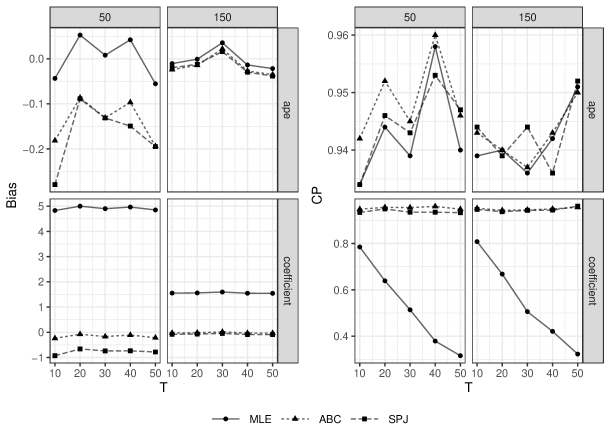
Figure A3: Dynamic: Two-way Fixed Effects — Predetermined Regressor

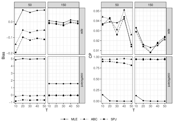
Figure A4: Dynamic: Two-way Fixed Effects — Exogenous Regressor

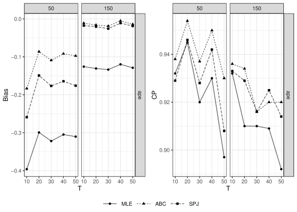
Figure A5: Dynamic: Two-way Fixed Effects — Exogenous Regressor (Long-Run)

Table A13: Dynamic: Two-way FEs — $z$, $N=50$

	Coefficients				APE
	Bias	Bias/SE	SE/SD	CP .95	Bias	Bias/SE	SE/SD	CP .95
	N = 50; T = 10
MLE	4.86	3.10	0.95	0.14	-0.02	-0.01	0.96	0.94
ABC	-0.21	-0.14	0.99	0.95	-0.14	-0.11	0.97	0.94
SPJ	-0.85	-0.56	0.96	0.90	-0.20	-0.14	0.96	0.94
	N = 50; T = 20
MLE	5.02	4.53	0.97	0.01	0.08	0.08	0.96	0.94
ABC	-0.06	-0.05	1.01	0.95	-0.05	-0.05	0.97	0.94
SPJ	-0.67	-0.62	0.97	0.90	-0.10	-0.10	0.95	0.94
	N = 50; T = 30
MLE	4.94	5.46	0.96	0.00	0.06	0.08	0.93	0.94
ABC	-0.13	-0.14	1.00	0.95	-0.07	-0.09	0.94	0.93
SPJ	-0.72	-0.82	0.96	0.88	-0.12	-0.15	0.93	0.93
	N = 50; T = 40
MLE	4.99	6.36	1.00	0.00	0.07	0.11	0.95	0.94
ABC	-0.09	-0.11	1.04	0.96	-0.06	-0.08	0.96	0.95
SPJ	-0.68	-0.90	1.03	0.86	-0.11	-0.15	0.94	0.94
	N = 50; T = 50
MLE	4.98	7.09	0.97	0.00	0.07	0.12	0.91	0.92
ABC	-0.10	-0.14	1.01	0.95	-0.05	-0.09	0.92	0.93
SPJ	-0.70	-1.02	0.96	0.81	-0.11	-0.18	0.89	0.91

Table A14: Dynamic: Two-way FEs — $z$, $N=100$

	Coefficients				APE
	Bias	Bias/SE	SE/SD	CP .95	Bias	Bias/SE	SE/SD	CP .95
	N = 100; T = 10
MLE	2.34	3.08	0.97	0.15	-0.02	-0.02	0.91	0.92
ABC	-0.07	-0.09	0.99	0.95	-0.05	-0.06	0.91	0.92
SPJ	-0.22	-0.29	0.98	0.94	-0.06	-0.08	0.91	0.92
	N = 100; T = 20
MLE	2.38	4.42	1.01	0.00	0.01	0.02	0.94	0.94
ABC	-0.03	-0.06	1.03	0.95	-0.02	-0.04	0.94	0.93
SPJ	-0.17	-0.32	1.02	0.94	-0.03	-0.06	0.93	0.93
	N = 100; T = 30
MLE	2.36	5.38	0.97	0.00	0.00	0.00	0.91	0.92
ABC	-0.05	-0.10	0.99	0.95	-0.03	-0.06	0.91	0.93
SPJ	-0.18	-0.41	0.96	0.92	-0.04	-0.09	0.90	0.92
	N = 100; T = 40
MLE	2.39	6.29	0.98	0.00	0.02	0.05	0.90	0.92
ABC	-0.02	-0.05	0.99	0.95	-0.01	-0.03	0.91	0.92
SPJ	-0.15	-0.40	0.97	0.93	-0.02	-0.06	0.89	0.92
	N = 100; T = 50
MLE	2.40	7.04	0.99	0.00	0.02	0.05	0.91	0.92
ABC	-0.01	-0.04	1.01	0.95	-0.01	-0.03	0.91	0.92
SPJ	-0.14	-0.43	0.99	0.92	-0.02	-0.06	0.90	0.92

Table A15: Dynamic: Two-way FEs — $z$, $N=150$

	Coefficients				APE
	Bias	Bias/SE	SE/SD	CP .95	Bias	Bias/SE	SE/SD	CP .95
	N = 150; T = 10
MLE	1.57	3.13	0.99	0.12	0.01	0.01	0.89	0.93
ABC	-0.01	-0.03	1.00	0.95	-0.00	-0.01	0.89	0.93
SPJ	-0.07	-0.15	0.99	0.94	-0.01	-0.02	0.89	0.93
	N = 150; T = 20
MLE	1.56	4.39	0.98	0.01	0.00	0.00	0.87	0.92
ABC	-0.02	-0.06	0.99	0.95	-0.01	-0.03	0.87	0.92
SPJ	-0.08	-0.21	0.97	0.94	-0.01	-0.04	0.87	0.91
	N = 150; T = 30
MLE	1.55	5.35	0.98	0.00	-0.01	-0.02	0.86	0.91
ABC	-0.03	-0.10	0.99	0.95	-0.02	-0.06	0.86	0.91
SPJ	-0.08	-0.29	0.98	0.94	-0.02	-0.08	0.85	0.91
	N = 150; T = 40
MLE	1.57	6.26	0.98	0.00	0.01	0.04	0.89	0.92
ABC	-0.01	-0.03	0.99	0.94	-0.00	-0.00	0.89	0.92
SPJ	-0.07	-0.26	0.98	0.94	-0.00	-0.02	0.89	0.92
	N = 150; T = 50
MLE	1.57	6.98	1.01	0.00	0.00	0.02	0.91	0.92
ABC	-0.01	-0.05	1.03	0.96	-0.01	-0.03	0.91	0.92
SPJ	-0.07	-0.30	1.01	0.94	-0.01	-0.05	0.90	0.92

Table A16: Dynamic: Two-way FEs — $y_{t-1}$, $N=50$

	Coefficients				APE
	Bias	Bias/SE	SE/SD	CP .95	Bias	Bias/SE	SE/SD	CP .95
	N = 50; T = 10
MLE	4.83	1.10	0.95	0.78	-0.04	-0.01	0.95	0.93
ABC	-0.24	-0.05	0.99	0.95	-0.18	-0.04	0.97	0.94
SPJ	-0.93	-0.21	0.96	0.93	-0.28	-0.06	0.94	0.93
	N = 50; T = 20
MLE	5.00	1.60	0.98	0.64	0.05	0.02	0.96	0.94
ABC	-0.08	-0.03	1.02	0.96	-0.09	-0.03	0.98	0.95
SPJ	-0.66	-0.21	1.00	0.95	-0.09	-0.03	0.96	0.95
	N = 50; T = 30
MLE	4.90	1.92	0.94	0.51	0.01	0.00	0.94	0.94
ABC	-0.17	-0.07	0.98	0.95	-0.13	-0.05	0.96	0.94
SPJ	-0.74	-0.29	0.95	0.94	-0.13	-0.05	0.94	0.94
	N = 50; T = 40
MLE	4.97	2.24	0.99	0.38	0.04	0.02	0.99	0.96
ABC	-0.11	-0.05	1.03	0.96	-0.10	-0.04	1.01	0.96
SPJ	-0.74	-0.34	1.00	0.94	-0.15	-0.07	0.99	0.95
	N = 50; T = 50
MLE	4.85	2.45	0.98	0.32	-0.06	-0.03	0.97	0.94
ABC	-0.22	-0.11	1.02	0.95	-0.19	-0.10	0.98	0.95
SPJ	-0.78	-0.40	1.01	0.93	-0.19	-0.10	0.97	0.95

Table A17: Dynamic: Two-way FEs — $y_{t-1}$, $N=100$

	Coefficients				APE
	Bias	Bias/SE	SE/SD	CP .95	Bias	Bias/SE	SE/SD	CP .95
	N = 100; T = 10
MLE	2.44	1.14	1.03	0.80	0.08	0.04	1.04	0.95
ABC	0.03	0.01	1.05	0.95	0.05	0.02	1.04	0.96
SPJ	-0.10	-0.05	1.04	0.95	0.06	0.03	1.04	0.95
	N = 100; T = 20
MLE	2.35	1.54	0.98	0.66	-0.03	-0.02	0.99	0.94
ABC	-0.06	-0.04	1.00	0.94	-0.06	-0.04	1.00	0.95
SPJ	-0.19	-0.13	0.99	0.94	-0.06	-0.04	0.99	0.94
	N = 100; T = 30
MLE	2.39	1.92	0.97	0.52	0.03	0.02	0.99	0.95
ABC	-0.02	-0.02	0.99	0.95	-0.00	-0.00	0.99	0.95
SPJ	-0.14	-0.11	0.96	0.94	-0.00	-0.00	0.97	0.95
	N = 100; T = 40
MLE	2.38	2.20	0.97	0.41	0.00	0.00	0.97	0.94
ABC	-0.03	-0.03	0.99	0.95	-0.03	-0.03	0.98	0.94
SPJ	-0.16	-0.15	0.98	0.94	-0.03	-0.03	0.97	0.94
	N = 100; T = 50
MLE	2.40	2.48	0.98	0.29	0.02	0.02	0.97	0.94
ABC	-0.01	-0.01	1.00	0.95	-0.01	-0.01	0.98	0.95
SPJ	-0.14	-0.15	0.97	0.93	-0.02	-0.02	0.96	0.93

Table A18: Dynamic: Two-way FEs — $y_{t-1}$, $N=150$

	Coefficients				APE
	Bias	Bias/SE	SE/SD	CP .95	Bias	Bias/SE	SE/SD	CP .95
	N = 150; T = 10
MLE	1.55	1.09	0.99	0.81	-0.01	-0.01	0.99	0.94
ABC	-0.03	-0.02	1.00	0.95	-0.02	-0.02	0.99	0.94
SPJ	-0.08	-0.06	0.99	0.95	-0.02	-0.01	0.98	0.94
	N = 150; T = 20
MLE	1.56	1.55	0.97	0.67	-0.00	-0.00	0.96	0.94
ABC	-0.02	-0.02	0.98	0.94	-0.01	-0.01	0.96	0.94
SPJ	-0.07	-0.07	0.97	0.94	-0.01	-0.01	0.96	0.94
	N = 150; T = 30
MLE	1.60	1.94	1.00	0.51	0.04	0.04	0.99	0.94
ABC	0.01	0.02	1.01	0.94	0.02	0.03	1.00	0.94
SPJ	-0.04	-0.05	1.01	0.94	0.02	0.02	0.99	0.94
	N = 150; T = 40
MLE	1.55	2.17	0.99	0.42	-0.01	-0.02	0.97	0.94
ABC	-0.03	-0.05	1.01	0.95	-0.03	-0.04	0.97	0.94
SPJ	-0.09	-0.13	0.99	0.94	-0.03	-0.04	0.96	0.94
	N = 150; T = 50
MLE	1.54	2.42	1.00	0.32	-0.02	-0.03	0.98	0.95
ABC	-0.04	-0.06	1.01	0.96	-0.04	-0.05	0.98	0.95
SPJ	-0.09	-0.15	1.00	0.96	-0.04	-0.06	0.97	0.95

Table A19: Dynamic: Two-way FEs — $z$, $N=50$ long-run

	APE
	Bias	Bias/SE	SE/SD	CP .95
	N = 50; T = 10
MLE	-0.40	-0.30	0.97	0.93
ABC	-0.18	-0.14	0.96	0.94
SPJ	-0.26	-0.19	0.95	0.93
	N = 50; T = 20
MLE	-0.30	-0.32	1.00	0.94
ABC	-0.09	-0.09	0.99	0.95
SPJ	-0.15	-0.16	0.97	0.95
	N = 50; T = 30
MLE	-0.32	-0.41	0.97	0.92
ABC	-0.11	-0.14	0.96	0.94
SPJ	-0.18	-0.23	0.93	0.93
	N = 50; T = 40
MLE	-0.30	-0.45	1.00	0.93
ABC	-0.09	-0.14	0.99	0.95
SPJ	-0.16	-0.24	0.97	0.94
	N = 50; T = 50
MLE	-0.31	-0.52	0.92	0.90
ABC	-0.10	-0.16	0.92	0.93
SPJ	-0.18	-0.29	0.88	0.91

Table A20: Dynamic: Two-way FEs — $z$, $N=100$ long-run

	APE
	Bias	Bias/SE	SE/SD	CP .95
	N = 100; T = 10
MLE	-0.20	-0.27	0.95	0.93
ABC	-0.05	-0.06	0.94	0.94
SPJ	-0.06	-0.08	0.94	0.94
	N = 100; T = 20
MLE	-0.19	-0.35	0.96	0.93
ABC	-0.03	-0.06	0.95	0.94
SPJ	-0.05	-0.09	0.94	0.94
	N = 100; T = 30
MLE	-0.19	-0.43	0.95	0.92
ABC	-0.03	-0.07	0.94	0.94
SPJ	-0.05	-0.11	0.93	0.93
	N = 100; T = 40
MLE	-0.18	-0.47	0.94	0.91
ABC	-0.02	-0.06	0.93	0.94
SPJ	-0.03	-0.09	0.92	0.94
	N = 100; T = 50
MLE	-0.17	-0.51	0.95	0.91
ABC	-0.02	-0.05	0.94	0.93
SPJ	-0.03	-0.09	0.93	0.93

Table A21: Dynamic: Two-way FEs — $z$, $N=150$ long-run

	APE
	Bias	Bias/SE	SE/SD	CP .95
	N = 150; T = 10
MLE	-0.13	-0.22	0.93	0.93
ABC	-0.01	-0.02	0.93	0.94
SPJ	-0.02	-0.03	0.92	0.93
	N = 150; T = 20
MLE	-0.13	-0.33	0.91	0.91
ABC	-0.02	-0.04	0.91	0.93
SPJ	-0.02	-0.05	0.90	0.93
	N = 150; T = 30
MLE	-0.13	-0.41	0.89	0.91
ABC	-0.02	-0.06	0.89	0.92
SPJ	-0.03	-0.08	0.88	0.92
	N = 150; T = 40
MLE	-0.12	-0.42	0.92	0.91
ABC	-0.01	-0.02	0.91	0.92
SPJ	-0.01	-0.04	0.91	0.92
	N = 150; T = 50
MLE	-0.13	-0.51	0.92	0.89
ABC	-0.01	-0.06	0.92	0.92
SPJ	-0.02	-0.07	0.91	0.91

C.3 Static: Three-way Fixed Effects

$$y_{ijt}=\mbox{\boldmath$\,{1}\!$}\left[\beta_{z}z_{ijt}+\psi_{jt}+\lambda_{it}+\mu_{ij}\geq\epsilon_{ijt}\right]\,,$$

where $\psi_{jt}\sim\mbox{$\mathrm{iid}.\ $}\mbox{$\mathcal{N}$}(0,1/24)$, $\lambda_{it}\sim\mbox{$\mathrm{iid}.\ $}\mbox{$\mathcal{N}$}(0,1/24)$, $\mu_{ij}\sim\mbox{$\mathrm{iid}.\ $}\mbox{$\mathcal{N}$}(0,1/24)$, and $\epsilon_{ijt}\sim\mbox{$\mathrm{iid}.\ $}\mbox{$\mathcal{N}$}(0,1)$. Further, $\beta_{z}=1$ and $z_{ijt}=0.5z_{ijt-1}+\psi_{jt}+\lambda_{it}+\mu_{ij}+\nu_{ijt}$, where $\nu_{ijt}\sim\mbox{$\mathrm{iid}.\ $}\mbox{$\mathcal{N}$}(0,0.5)$, $z_{ij0}\sim\mbox{$\mathrm{iid}.\ $}\mbox{$\mathcal{N}$}(0,1)$.

Table A22: Static: Three-way FEs — $z$, $N=50$

	Coefficients				APE
	Bias	Bias/SE	SE/SD	CP .95	Bias	Bias/SE	SE/SD	CP .95
	N = 50; T = 10
MLE	21.50	11.16	0.85	0.00	0.99	0.72	0.93	0.86
ABC	-1.46	-0.84	1.02	0.87	-1.33	-0.92	1.00	0.84
SPJ	-11.69	-7.10	0.69	0.00	-0.35	-0.24	0.80	0.88
	N = 50; T = 20
MLE	12.15	10.11	0.89	0.00	0.39	0.42	1.00	0.93
ABC	-0.59	-0.53	0.99	0.91	-0.45	-0.47	1.04	0.92
SPJ	-3.99	-3.60	0.85	0.10	-0.65	-0.68	0.91	0.87
	N = 50; T = 30
MLE	9.51	10.07	0.90	0.00	0.27	0.36	0.98	0.94
ABC	-0.40	-0.44	0.98	0.93	-0.25	-0.32	1.00	0.94
SPJ	-2.34	-2.63	0.91	0.28	-0.45	-0.58	0.93	0.90
	N = 50; T = 40
MLE	8.36	10.40	0.95	0.00	0.24	0.37	1.03	0.93
ABC	-0.24	-0.32	1.02	0.94	-0.15	-0.22	1.04	0.95
SPJ	-1.65	-2.17	0.94	0.42	-0.31	-0.47	0.96	0.92
	N = 50; T = 50
MLE	7.60	10.70	0.93	0.00	0.19	0.31	1.05	0.95
ABC	-0.23	-0.34	0.99	0.94	-0.14	-0.23	1.06	0.95
SPJ	-1.39	-2.05	0.93	0.44	-0.28	-0.46	0.97	0.92

Table A23: Static: Three-way FEs — $z$, $N=100$

	Coefficients				APE
	Bias	Bias/SE	SE/SD	CP .95	Bias	Bias/SE	SE/SD	CP .95
	N = 100; T = 10
MLE	17.62	19.04	0.86	0.00	0.56	0.79	1.01	0.88
ABC	-0.86	-1.02	1.01	0.83	-1.05	-1.44	1.05	0.71
SPJ	-8.01	-9.78	0.73	0.00	0.46	0.62	0.87	0.87
	N = 100; T = 20
MLE	9.12	15.69	0.90	0.00	0.22	0.47	1.00	0.92
ABC	-0.29	-0.53	0.97	0.91	-0.27	-0.57	1.02	0.92
SPJ	-2.42	-4.41	0.88	0.01	-0.24	-0.49	0.93	0.90
	N = 100; T = 30
MLE	6.68	14.60	0.96	0.00	0.13	0.33	1.00	0.94
ABC	-0.18	-0.40	1.01	0.94	-0.14	-0.36	1.01	0.94
SPJ	-1.22	-2.77	0.94	0.22	-0.18	-0.46	0.95	0.91
	N = 100; T = 40
MLE	5.51	14.18	0.95	0.00	0.08	0.24	0.99	0.95
ABC	-0.14	-0.37	1.00	0.94	-0.10	-0.30	0.99	0.93
SPJ	-0.81	-2.14	0.95	0.44	-0.15	-0.44	0.95	0.91
	N = 100; T = 50
MLE	4.85	14.10	0.91	0.00	0.06	0.21	0.99	0.94
ABC	-0.11	-0.32	0.95	0.92	-0.07	-0.24	1.00	0.94
SPJ	-0.60	-1.78	0.90	0.56	-0.12	-0.38	0.95	0.93

Table A24: Static: Three-way FEs — $z$, $N=150$

	Coefficients				APE
	Bias	Bias/SE	SE/SD	CP .95	Bias	Bias/SE	SE/SD	CP .95
	N = 150; T = 10
MLE	16.39	26.88	0.88	0.00	0.41	0.84	0.99	0.86
ABC	-0.73	-1.29	1.02	0.76	-1.01	-2.01	1.02	0.49
SPJ	-7.12	-13.07	0.73	0.00	0.63	1.24	0.85	0.73
	N = 150; T = 20
MLE	8.16	21.28	0.97	0.00	0.18	0.54	1.02	0.92
ABC	-0.22	-0.60	1.04	0.92	-0.24	-0.72	1.03	0.89
SPJ	-2.06	-5.66	0.91	0.00	-0.15	-0.45	0.92	0.90
	N = 150; T = 30
MLE	5.78	19.17	0.97	0.00	0.10	0.37	1.01	0.95
ABC	-0.12	-0.41	1.02	0.94	-0.11	-0.41	1.02	0.94
SPJ	-0.98	-3.36	0.95	0.09	-0.13	-0.47	0.97	0.92
	N = 150; T = 40
MLE	4.64	18.08	0.97	0.00	0.05	0.22	1.03	0.94
ABC	-0.10	-0.40	1.01	0.93	-0.08	-0.36	1.03	0.94
SPJ	-0.62	-2.46	0.96	0.32	-0.11	-0.46	0.99	0.92
	N = 150; T = 50
MLE	4.01	17.65	1.01	0.00	0.05	0.24	1.01	0.95
ABC	-0.06	-0.27	1.05	0.95	-0.05	-0.22	1.01	0.95
SPJ	-0.42	-1.89	0.98	0.53	-0.07	-0.36	0.97	0.92

Appendix D Application

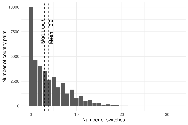
Figure A6: Distribution of frequency of switches between zero and non-zero trade.

Table A25: Homogeneity Test: Split-Panel Jackknife

	$I$	$J$	$T$
(2)	175.055	70.700	-
	(0.000)	(0.000)	(-)
(3)	56.681	72.546	-
	(0.000)	(0.000)	(-)
(4)	14.388	23.684	73.773
	(0.002)	(0.000)	(0.000)
(5)	26.085	20.669	72.056
	(0.000)	(0.000)	(0.000)
Notes: Test statistics of Wald tests for equality of structural parameters across sub panels splitted by $I$, $J$ and $T$; p-values in parantheses.

Table A26: Probit Estimation: Coefficients

	Dependent variable: $y_{ijt}$
	(1)	(2)	(3)	(4)	(5)
$y_{ij(t-1)}$	-	-	1.752***	-	1.169***
	(-)	(-)	(0.004)	(-)	(0.005)
	-	-	1.801***	-	1.090***
	(-)	(-)	(0.004)	(-)	(0.005)
log(Distance)	-	-0.818***	-0.530***	-	-
	(-)	(0.003)	(0.003)	(-)	(-)
	-0.711***	-0.836***	-0.546***	-	-
	(0.002)	(0.003)	(0.003)	(-)	(-)
Land border	-	0.140***	0.078***	-	-
	(-)	(0.014)	(0.016)	(-)	(-)
	0.169***	0.149***	0.089***	-	-
	(0.013)	(0.014)	(0.016)	(-)	(-)
Legal	-	0.032***	0.022***	-	-
	(-)	(0.004)	(0.004)	(-)	(-)
	0.024***	0.034***	0.023***	-	-
	(0.004)	(0.004)	(0.004)	(-)	(-)
Language	-	0.410***	0.271***	-	-
	(-)	(0.005)	(0.006)	(-)	(-)
	0.368***	0.420***	0.280***	-	-
	(0.005)	(0.005)	(0.006)	(-)	(-)
Colonial ties	-	0.297***	0.182***	-	-
	(-)	(0.006)	(0.007)	(-)	(-)
	0.268***	0.302***	0.186***	-	-
	(0.006)	(0.006)	(0.007)	(-)	(-)
Currency union	-	0.555***	0.355***	0.276***	0.195***
	(-)	(0.014)	(0.016)	(0.035)	(0.038)
	0.356***	0.571***	0.370***	0.308***	0.228***
	(0.012)	(0.014)	(0.017)	(0.036)	(0.038)
FTA	-	0.310***	0.199***	0.102***	0.069***
	(-)	(0.007)	(0.008)	(0.015)	(0.016)
	0.265***	0.313***	0.200***	0.101***	0.075***
	(0.006)	(0.007)	(0.008)	(0.015)	(0.015)
WTO / GATT	-	0.196***	0.127***	0.105***	0.076***
	(-)	(0.007)	(0.008)	(0.014)	(0.015)
	0.258***	0.200***	0.131***	0.113***	0.089***
	(0.004)	(0.007)	(0.008)	(0.014)	(0.015)
Fixed effects	$i,j,t$	$it,jt$	$it,jt$	$it,jt,ij$	$it,jt,ij$
Sample size	1652296	1652296	1613354	1652296	1613354
Deviance	11.65$\times$104	9.90$\times$104	7.17$\times$104	6.50$\times$104	5.76$\times$104
Notes: Column (1) uncorrected coefficients, columns (2) - (5) bias-corrected coefficients (bold font) and uncorrected coefficients (standard font). Columns (4) and (5) bias-corrected with $L=2$. Standard errors in parenthesis. ${}^{***}p<0.01$, ${}^{**}p<0.05$, ${}^{*}p<0.1$

Table A27: Logit Estimation with Different Bandwidths: Bias-Corrected Average Partial Effects

	Dependent variable: $y_{ijt}$
	$L=1$		$L=2$		$L=3$		$L=4$
	direct	long-run	direct	long-run	direct	long-run	direct	long-run
$y_{ij(t-1)}$	0.163***	-	0.169***	-	0.172***	-	0.173***
	(0.001)	(-)	(0.001)	(-)	(0.001)	(-)	(0.001)	(-)
Currency union	0.023***	0.035***	0.022***	0.035***	0.022***	0.035***	0.022***	0.035***
	(0.004)	(0.006)	(0.004)	(0.006)	(0.004)	(0.006)	(0.004)	(0.006)
FTA	0.008***	0.013***	0.008***	0.013***	0.008***	0.013***	0.008***	0.013***
	(0.002)	(0.002)	(0.002)	(0.002)	(0.002)	(0.002)	(0.002)	(0.002)
WTO/GATT	0.009***	0.014***	0.009***	0.014***	0.009***	0.014***	0.009***	0.014***
	(0.001)	(0.002)	(0.001)	(0.002)	(0.001)	(0.002)	(0.001)	(0.002)
Notes: All columns include Origin $\times$ Year, Destination $\times$ Year and Origin $\times$ Destination fixed effects. Standard errors in parenthesis. ${}^{***}p<0.01$, ${}^{**}p<0.05$, ${}^{*}p<0.1$

References

- [1] George Alessandria and Horag Choi “Do Sunk Costs of Exporting Matter for Net Export Dynamics?” In Quarterly Journal of Economics 122.1, 2007, pp. 289–336
- [2] James E. Anderson and Eric Wincoop “Gravity with Gravitas: A Solution to the Border Puzzle” In American Economic Review 93.1, 2003, pp. 170–192
- [3] James E. Anderson and Yoto V. Yotov “Pound for Pound Export Diversification” In NBER Working Paper 28277, 2020
- [4] Scott L. Baier and Jeffrey H. Bergstrand “Do Free Trade Agreements Actually Increase Members’ International Trade?” In Journal of International Economics 71.1, 2007, pp. 72–95
- [5] Laszlo Balazsi, Laszlo Matyas and Tom Wansbeek “The Estimation of Multidimensional Fixed Effects Panel Data Models” In Econometric Reviews 37.3 Taylor & Francis, 2018, pp. 212–227
- [6] Badi H. Baltagi, Peter Egger and Michael Pfaffermayr “A Generalized Design for Bilateral Trade Flow Models” In Economics Letters 80.3, 2003, pp. 391–397
- [7] Nicolas Berman, Vincent Rebeyrol and Vincent Vicard “Demand Learning and Firm Dynamics: Evidence from Exporters” In Review of Economics and Statistics 101.1 MIT Press One Rogers Street, Cambridge, MA 02142-1209USAjournals-info@mit.edu, 2019, pp. 91–106
- [8] Andrew B. Bernard, Esther Ann Bøler, Renzo Massari, Jose-Daniel Reyes and Daria Taglioni “Exporter Dynamics and Partial-Year Effects” In American Economic Review 107.10, 2017, pp. 3211–3228
- [9] Andrew B. Bernard and J. Jensen “Why Some Firms Export” In Review of Economics and Statistics 86.2, 2004, pp. 561–569
- [10] Martin Browning and Jesus M. Carro “Heterogeneity in Dynamic Discrete Choice Models” In Econometrics Journal 13.1, 2010, pp. 1–39
- [11] Jesus M. Carro “Estimating Dynamic Panel Data Discrete Choice Models with Fixed Effects” In CEMFI Working Paper 0304, 2003
- [12] Karyne B. Charbonneau “Multiple Fixed Effects in Binary Response Panel Data Models” In The Econometrics Journal 20.3 Wiley/Blackwell (10.1111), 2017, pp. S1–S13
- [13] Maddalena Conte, Pierre Cotterlaz and Thierry Mayer, 2021
- [14] Mario Cruz-Gonzalez, Iván Fernández-Val and Martin Weidner “Bias Corrections for Probit and Logit Models with Two-Way Fixed Effects” In Stata Journal 17.3, 2017, pp. 517–545
- [15] Daniel Czarnowske and Amrei Stammann “Binary Choice Models with High-Dimensional Individual and Time Fixed Effects” In Unpublished Working Paper, 2019
- [16] Sanghamitra Das, Mark J Roberts and James R Tybout “Market Entry Costs, Producer Heterogeneity, and Export Dynamics” In Econometrica 75.3, 2007, pp. 837–873
- [17] Geert Dhaene and Koen Jochmans “Split-Panel Jackknife Estimation of Fixed-Effect Models” In Review of Economic Studies 82.3, 2015, pp. 991–1030
- [18] Jonathan Eaton and Samuel Kortum “Technology, Geography, and Trade” In Econometrica 70.5, 2002, pp. 1741–1779
- [19] Jonathan Eaton, Samuel Kortum and Francis Kramarz “An Anatomy of International Trade: Evidence From French Firms” In Econometrica 79.5, 2011, pp. 1453–1498
- [20] Jonathan Eaton, Samuel Kortum and Sebastian Sotelo “International Trade: Linking Micro and Macro” In Advances in Economics and Econometrics: Tenth World Congress, Volume II: Applied Economics Cambridge University Press, 2013, pp. 329–370
- [21] Peter Egger and Mario Larch “An Assessment of the Europe Agreements’ Effects on Bilateral Trade, GDP, and Welfare” In European Economic Review 55.2, 2011, pp. 263–279
- [22] Peter Egger, Mario Larch, Kevin E Staub and Rainer Winkelmann “The Trade Effects of Endogenous Preferential Trade Agreements” In American Economic Journal: Economic Policy 3.3, 2011, pp. 113–143
- [23] Robert C. Feenstra “Advanced International Trade: Theory and Evidence” Princeton, NJ: Princeton University Press, 2004
- [24] Iván Fernández-Val and Martin Weidner “Individual and Time Effects in Nonlinear Panel Models with Large N, T” In Journal of Econometrics 192.1, 2016, pp. 291–312
- [25] Iván Fernández-Val and Martin Weidner “Fixed Effects Estimation of Large-T Panel Data Models” In Annual Review of Economics 10.1 Annual Reviews 4139 El Camino Way, PO Box 10139, Palo Alto, California 94303-0139, USA, 2018, pp. 109–138
- [26] Simen Gaure “OLS with Multiple High Dimensional Category Variables” In Computational Statistics & Data Analysis 66 North-Holland, 2013, pp. 8–18
- [27] Paulo Guimarães and Pedro Portugal “A Simple Feasible Procedure to Fit Models with High-Dimensional Fixed Effects” In Stata Journal 10.4, 2010, pp. 628–649
- [28] Jinyong Hahn and Guido Kuersteiner “Asymptotically Unbiased Inference for a Dynamic Panel Model with Fixed Effects when Both n and T Are Large” In Econometrica 70.4 Wiley/Blackwell (10.1111), 2002, pp. 1639–1657
- [29] Jinyong Hahn and Guido Kuersteiner “Bandwidth Choice for Bias Estimators in Dynamic Nonlinear Panel Models” In Unpublished Working Paper, 2007
- [30] Jinyong Hahn and Whitney Newey “Jackknife and Analytical Bias Reduction for Nonlinear Panel Models” In Econometrica 72.4 Wiley/Blackwell (10.1111), 2004, pp. 1295–1319
- [31] Israel Halperin “The Product of Projection Operators” In Acta Sci. Math.(Szeged) 23.1-2, 1962, pp. 96–99
- [32] Keith Head and Thierry Mayer “Gravity Equations: Workhorse, Toolkit, and Cookbook” In Handbook of International Economics 4 North Holland, 2014, pp. 131–195
- [33] Keith Head, Thierry Mayer and John Ries “The Erosion of Colonial Trade Linkages after Independence” In Journal of International Economics 81.1, 2010, pp. 1–14
- [34] James J. Heckman “Statistical Models for Discrete Panel Data” In Structural Analysis of Discrete Data with Econometric Applications Cambridge, MA: MIT Press, 1981
- [35] Elhanan Helpman, Marc J. Melitz and Yona Rubinstein “Estimating Trade Flows: Trading Partners and Trading Volumes” In Quarterly Journal of Economics 123.2, 2008, pp. 441–487
- [36] Paul Krugman “Scale Economies, Product Differentiation, and the Pattern of Trade” In American Economic Review 70.5, 1980, pp. 950–959
- [37] Marc J. Melitz “The Impact of Trade on Intra-Industry Reallocations and Aggregate Industry Productivity” In Econometrica 71.6, 2003, pp. 1695–1725
- [38] J. Neyman and Elisabeth L. Scott “Consistent Estimates Based on Partially Consistent Observations” In Econometrica 16.1, 1948, pp. 1–32
- [39] Stephen Nickell “Biases in Dynamic Models with Fixed Effects” In Econometrica 49.6, 1981, pp. 1417–1426
- [40] Paul Piveteau “An Empirical Dynamic Model of Trade with Consumer Accumulation” In Unpublished Working Paper, 2019
- [41] Stephen J. Redding and Anthony J. Venables “Economic Geography and International Inequality” In Journal of International Economics 62.1, 2004, pp. 53–82
- [42] Mark J Roberts and James R Tybout “The Decision to Export in Colombia: An Empirical Model of Entry with Sunk Costs” In American Economic Review 87.4, 1997, pp. 545–564
- [43] Kim J. Ruhl and Jonathan L. Willis “New Exporter Dynamics” In International Economic Review 58.3 John Wiley & Sons, Ltd (10.1111), 2017, pp. 703–726
- [44] J… Santos Silva and Silvana Tenreyro “The Log of Gravity” In Review of Economics and Statistics 88.4, 2006, pp. 641–658
- [45] J… Santos Silva, Silvana Tenreyro and Kehai Wei “Estimating the Extensive Margin of Trade” In Journal of International Economics 93.1 Elsevier, 2014, pp. 67–75
- [46] Amrei Stammann “Fast and Feasible Estimation of Generalized Linear Models with High-Dimensional k-way Fixed Effects” In Unpublished Working Paper, 2018
- [47] John Von Neumann “Functional Operators. Vol. II. The geometry of orthogonal spaces, volume 22 (reprint of 1933 notes) of Annals of Math.” Princeton University Press, 1950
- [48] Martin Weidner and Thomas Zylkin “Bias and Consistency in Three-way Gravity Models” In Unpublished Working Paper, 2020