Differentiating through Log-Log Convex Programs

Abstract

We show how to efficiently compute the derivative (when it exists) of the solution map of log-log convex programs (LLCPs). These are nonconvex, nonsmooth optimization problems with positive variables that become convex when the variables, objective functions, and constraint functions are replaced with their logs. We focus specifically on LLCPs generated by disciplined geometric programming, a grammar consisting of a set of atomic functions with known log-log curvature and a composition rule for combining them. We represent a parametrized LLCP as the composition of a smooth transformation of parameters, a convex optimization problem, and an exponential transformation of the convex optimization problem’s solution. The derivative of this composition can be computed efficiently, using recently developed methods for differentiating through convex optimization problems. We implement our method in CVXPY, a Python-embedded modeling language and rewriting system for convex optimization. In just a few lines of code, a user can specify a parametrized LLCP, solve it, and evaluate the derivative or its adjoint at a vector. This makes it possible to conduct sensitivity analyses of solutions, given perturbations to the parameters, and to compute the gradient of a function of the solution with respect to the parameters. We use the adjoint of the derivative to implement differentiable log-log convex optimization layers in PyTorch and TensorFlow. Finally, we present applications to designing queuing systems and fitting structured prediction models.

1 Introduction

1.1 Log-log convex programs

A log-log convex program (LLCP) is a mathematical optimization problem in which the variables are positive, the objective and inequality constraint functions are log-log convex, and the equality constraint functions are log-log affine. A function $f:D\subseteq{\mbox{\bf R}}^{n}_{++}\to{\mbox{\bf R}}_{++}$ (${\mbox{\bf R}}_{++}$ denotes the positive reals) is log-log convex if for all $x$, $y\in D$ and $\theta\in[0,1]$,

$$f(x^{\theta}\circ y^{1-\theta})\leq f(x)^{\theta}\circ f(y)^{1-\theta},$$

and $f$ is log-log affine if the inequality holds with equality (the powers are meant elementwise and $\circ$ denotes the elementwise product). Similarly, $f$ is log-log concave if the inequality holds when its direction is reversed. A LLCP has the standard form

$$\begin{array}[]{ll}\mbox{minimize}&f_{0}(x)\\ \mbox{subject to}&f_{i}(x)\leq 1,\quad i=1,\ldots,m_{1}\\ &g_{i}(x)=1,\quad i=1,\ldots,m_{2},\end{array}$$ (1)

where $x\in{\mbox{\bf R}}^{n}_{++}$ is the variable, the functions $f_{i}$ are log-log convex, and $g_{i}$ are log-log affine [ADB19]. A value of the variable is a solution of the problem if it minimizes the objective function, among all values satisfying the constraints.

The problem (1) is not convex, but it can be readily transformed to a convex optimization problem. We make the change of variables $u=\log x$, replace each function $f$ appearing in the LLCP with its log-log transformation, defined by $F(u)=\log f(e^{u})$, and replace the right-hand sides of the constraints with $0$. Because the log-log transformation of a log-log convex function is convex, we obtain an equivalent convex optimization problem. This means that LLCPs can be solved efficiently and globally, using standard algorithms for convex optimization [BV04].

The class of log-log convex programs is large, including many interesting problems as special cases. Geometric programs (GPs) form a well-studied subclass of LLCPs; these are LLCPs in which the equality constraint functions are monomials, of the form $x\mapsto cx_{1}^{a_{1}}x_{2}^{a_{2}}\cdots x_{n}^{a_{n}}$, with $a_{1},\ldots a_{n}\in{\mbox{\bf R}}$ and $c\in{\mbox{\bf R}}_{++}$, and the objective and inequality constraint functions are sums of monomials, called posynomials [DPZ67, Boy+07]. GPs have found application in digital and analog circuit design [Boy+05, HBL01, Li+04, XPB04], aircraft design [HA14, BH18, SBH18], epidemiology [Pre+14, OP16], chemical engineering [Cla84], communication systems [KB02, Chi05, Chi+07], control [OKL19], project management [Ogu+19], and data fitting [HKA16, CGP19]; for more, see [ADB19, §1.1] and [Boy+07, §10.3]

In this paper we consider LLCPs in which the objective and constraint functions are parametrized, and we are interested in computing how a solution to an LLCP changes with small perturbations to the parameters. For example, in a GP, the parameters are the coefficients and exponents appearing in monomials and posynomials. While sensitivity analysis of GPs is well-studied [DK77, Dem82, Kyp88, Kyp90], sensitivity analysis of LLCPs has not, to our knowledge, previously appeared in the literature. Our emphasis in this paper is on practical computation, instead of a theoretical characterization of the differentiability of the solution map.

1.2 Solution maps and sensitivity analysis

An optimization problem can be viewed as a multivalued function mapping parameters to the set of solutions; this set might contain zero, one, or many elements. In neighborhoods where this solution map is single-valued, it is an implicit function of the parameters [DR09]. In these neighborhoods it is meaningful to discuss how perturbations in the parameters affect the solution. The point of this paper is to efficiently calculate the sensitivity of the solution of an LLCP to these perturbations, by implicitly differentiating the solution map; this calculation also lets us compute the gradient of a scalar-valued function of the solution, with respect to the parameters.

There is a large body of work on the sensitivity analysis of optimization problems, going back multiple decades. Early papers include [FM68] and [Fia76], which apply the implicit function theorem to the first-order KKT conditions of a nonlinear program with twice-differentiable objective and constraint functions. A similar method was applied to GPs in [Kyp88, Kyp90]. Much of the work on sensitivity analysis of GPs focuses on the special structure of the dual program (e.g., [DPZ67, Dem82]). Various results on sensitivity analyses of optimization problems, including nonlinear programs, semidefinite programs, and semi-infinite programs, are collected in [BS00].

Recently, a series of papers developed methods to calculate the derivative of convex optimization problems, in which the objective and constraint functions may be nonsmooth. The paper [BMB19] phrased a convex cone program as the problem of finding a zero of a certain residual map, and the papers [Agr+19b, Amo19] showed how to differentiate through cone programs (when certain regularity conditions are satisfied) by a straightforward application of the implicit function theorem to this residual map. In [Agr+19a], a method was developed to differentiate through high-level descriptions of convex optimization problems, specified in a domain-specific language for convex optimization. The method from [Agr+19a] reduces convex optimization problems to cone programs in an efficient and differentiable way. The present paper can be understood as an analogue of [Agr+19a] for LLCPs.

1.3 Domain-specific languages for optimization

Log-log convex functions satisfy an important composition rule, analogous to the composition rule for convex functions. Suppose $h:D\subseteq{\mbox{\bf R}}^{m}_{++}\to{\mbox{\bf R}}_{++}\cup\{+\infty\}$ is log-log convex, and let $[I_{1},I_{2},I_{3}]$ be a partition of $\{1,2,\ldots,m\}$ such that $f$ is nondecreasing in the arguments index by $I_{1}$ and nonincreasing in the arguments indexed by $I_{2}$. If $g$ maps a subset of ${\mbox{\bf R}}^{n}_{++}$ into ${\mbox{\bf R}}^{m}_{++}$ such that its components $g_{i}$ are log-log convex for $i\in I_{1}$, log-log concave for $i\in I_{2}$, and log-log affine for $i\in I_{3}$, then the composition

$$f=h\circ g$$

is log-log convex. An analogous rule holds for log-log concave functions.

When combined with a set of atomic functions with known log-log curvature and per-argument monotonicities, this composition rule defines a grammar for log-log convex functions, i.e., a rule for combining atomic functions to create other functions with verifiable log-log curvature. This is the basis of disciplined geometric programming (DGP), a grammar for LLCPs [ADB19]. In addition to compositions of atomic functions, DGP also includes LLCPs as valid expressions, permitting the minimization of a log-log convex function (or maximization of a log-log concave function), subject to inequality constraints $f(x)\leq g(x)$, where $f$ is log-log convex and $g$ is log-log concave, and equality constraints $f(x)=g(x)$, where $f$ and $g$ are log-log affine. In §2.2, we extend DGP to include parametrized LLCPs.

The class of DGP problems is a subclass of LLCPs. Depending on the choice of atomic functions, or atoms, this class can be made quite large. For example, taking powers, products, and sums as the atoms yields GP; adding the maximum operator yields generalized geometric programming (GGP). Several other atoms can be added, such as the exponential function, the logarithm, and functions of elementwise positive matrices, yielding a subclass of LLCPs strictly larger than GGP (see [ADB19, §3] for examples). In this paper we restrict our attention to LLCPs generated by DGP; this is not a limitation in practice, since the atom library is extensible.

DGP can be used as the grammar for a domain-specific language (DSL) for log-log convex optimization. A DSL for log-log convex optimization parses LLCPs written in a human readable form, rewrites them into canonical forms, and compiles the canonical forms into numerical data for low-level numerical solvers. Because valid problems are guaranteed to be LLCPs, the DSL can guarantee that the compilation and the numerical solve are correct (i.e., valid problems can be solved globally). By abstracting away the numerical solver, DSLs make optimization accessible, vastly decreasing the time between formulating a problem and solving it with a computer. Examples of DSLs for LLCPs include CVXPY [DB16, Agr+18] and CVXR [FNB17]; additionally, CVX [GB14], GPKit [BDH20], and Yalmip [Löf04] support GPs.

Finally, we mention that modern DSLs for convex optimization are based on disciplined convex programming (DCP) [GBY06], which is analogous to DGP. CVXPY, CVXR, CVX, and Convex.jl [Ude+14] support convex optimization using DCP as the grammar. In [Agr+19a], a method for differentiating through parametrized DCP problems was developed; this method was implemented in CVXPY, and PyTorch [Pas+19] and TensorFlow [Aba+16, Agr+19d] wrappers for differentiable CVXPY problems were implemented in a Python package called CVXPY Layers.

1.4 This paper

In this paper we describe how to efficiently compute the derivative of a LLCP, when it exists, specifically considering LLCPs generated by DGP. In particular, we show how to evaluate the derivative (and its adjoint) of the solution map of an LLCP at a vector. To do this, we first extend the DGP ruleset to include parameters as atoms, in §2. Then, in §3, we represent a parametrized DGP problem by the composition of a smooth transformation of parameters, a parametrized DCP problem, and an exponential transformation of the DCP problem’s solution. We differentiate through this composition using recently developed methods from [BMB19, Agr+19b, Agr+19a] to differentiate through the DCP problem. Unlike prior work on sensitivity analysis of GPs, in which the objective and constraint functions are smooth, our method extends to problems with nonsmooth objective and constraints.

We implement the derivative of LLCPs as an abstract linear operator in CVXPY. In just a few lines of code, users can conduct first-order sensitivity analyses to examine how the values of variables would change given small perturbations of the parameters. Using the adjoint of the derivative operator, users can compute the gradient of a function of the solution to a DGP problem, with respect to the parameters. For convenience, we implement PyTorch and TensorFlow wrappers of the adjoint derivative in CVXPY Layers, making it easy to use log-log convex optimization problems as tunable layers in differentiable programs or neural networks. For our implementation, the overhead in differentiating through the DSL (which rewrites the high-level description of a problem into low-level numerical data for a solver, and retrieves a solution for the original problem from a solution from the solver) is small compared to the time spent in the numerical solver. In particular, the mapping from the transformed parameters to the numerical solver data is affine and can be represented compactly by a sparse matrix, and so can be evaluated quickly. Our implementation is described and illustrated with usage examples in §4.

In §5, we present two simple examples, in which we apply a sensitivity analysis to the design of an $M/M/N$ queuing system, and fit a structured prediction model.

1.5 Related work

Automatic differentiation.

Automatic differentiation (AD) is a family of methods that use the chain rule to algorithmically compute exact derivatives of compositions of differentiable functions, dating back to the 1950s [Bed+59]. There are two main types of AD. Reverse-mode AD computes the gradient of a scalar-valued composition of differentiable functions by applying the adjoint of the intermediate derivatives to the sensitivities of their outputs, while forward-mode AD computes applies the derivative of the composition to a vector of perturbations in the inputs [GW08]. In AD, derivatives are typically implemented as abstract linear maps, i.e., methods for applying the derivative and its adjoint at a vector; the derivative matrices of the intermediate functions are not materialized, i.e., formed or stored as arrays.

Recently, many high-quality open-source implementations of AD were made available. Examples include PyTorch [Pas+19], TensorFlow [Aba+16, Agr+19d], JAX [FJL18], and Zygote [Inn19]. These AD tools are used widely, especially to train machine learning models such as neural networks.

Optimization layers.

Implementing the derivative and its adjoint of an optimization problem makes it possible to implement the problem as a differentiable function in AD software. These differentiable solution maps are sometimes called optimization layers in the machine learning community. Many specific optimization layers have been implemented, including QP layers [AK17], convex optimization layers [Agr+19a], and nonlinear program layers [GHC19]. Optimization layers have found several applications in, e.g., computer graphics [GJF20], control [Agr+19c, de ̵+18, Amo+18, BB20], data fitting and classification [BB20a], game playing [LFK18], and combinatorial tasks [Ber+20].

While some optimization layers are implemented by differentiating through each step of an iterative algorithm (known as unrolling), we emphasize that in this paper, we differentiate through LLCPs analytically, without unrolling an optimization algorithm, and without tracing each step of the DSL.

Numerical solvers.

A numerical solver is an implementation of an optimization algorithm, specialized to a specific subclass of optimization problems. DSLs like CVXPY rewrite high-level descriptions of optimization problems to the rigid low-level formats required by solvers. While some solvers have been implemented specifically for GPs [Boy+07, §10.2], LLCPs (and GPs) can just as well be solved by generic solvers for convex cone programs that support the exponential cone. Our implementation reduces LLCPs to cone programs and solves them using SCS [O’D+16], an ADMM-based solver for cone programs. In principle, our method is compatible with other conic solvers as well, such as ECOS [DCB13] and MOSEK [ApS19].

2 Disciplined geometric programming

The DGP ruleset for unparametrized LLCPs was given in §1.3. Here, we remark on the types of atoms under consideration, and we extend DGP to include parameters as atoms. We then give several examples of parametrized, DGP-compliant expressions.

2.1 Atom library

The class of LLCPs producible using DGP depends on the atom library. We make a few standard assumptions on this library, limiting our attention to atoms that can be implemented in a DSL for convex optimization. In particular, we assume that the log-log transformation of each DGP atom (or its epigraph) can be represented in a DCP-compliant fashion, using DCP atoms. For example, this means that if the product is a DGP atom, then we require that the sum (which is its log-log transformation) to be a DCP atom. In turn, we assume that the epigraph of each DCP atom can be represented using the standard convex cones (i.e., the zero cone, the nonnegative orthant, the second-order cone, the exponential cone, and the semidefinite cone).

For simplicity, the reader may assume that the atoms under consideration are the ones listed in the DGP tutorial at

https://www.cvxpy.org.

The subclass of LLCPs generated by these atoms is a superset of GGPs, because it includes the product, sum, power, and maximum as atoms. It also includes other basic functions, such as the ratio, difference, exponential, logarithm, and entropy, and functions of elementwise positive matrices, such as the spectral radius and resolvent.

2.2 Parameters

We extend the DGP ruleset to include parameters as atoms by defining the curvature of parameters, and defining the curvature of a parametrized power atom. Like unparametrized expressions, a parametrized expression is log-log convex under DGP if can be generated by the composition rule.

Curvature.

The curvature of a positive parameter is log-log affine. Parameters that are not positive have unknown log-log curvature.

The power atom.

The power atom $f(x;a)=x^{a}$ is log-log affine if the exponent $a$ is a fixed numerical constant, or if $a$ is parameter and the argument $x$ is not parametrized. If $a$ is a parameter, it need not be positive. The exponent $a$ is not an argument of the power atom, i.e., DGP does not allow for the exponent to be a composition of atoms.

These rules ensure that a parametrized DGP problem can be reduced to a parametrized DCP problem, as explained in §3.1. (This, in turn, will simplify the calculation of the derivative of the solution map.) These rules are similar to the rules for parameters from [Agr+19a], in which a method for differentiating through parametrized DCP problems was developed. They are are not too restrictive; e.g., they permit taking the coefficients and exponents in a GP as parameters. We now give several examples of the kinds of parametrized expressions that can be constructed using DGP.

2.3 Examples

Example 1.

Consider a parametrized monomial

$$cx_{1}^{a_{1}}x_{2}^{a_{2}}\cdots x_{n}^{a_{n}},$$

where $x\in{\mbox{\bf R}}^{n}_{++}$ is the variable and $c\in{\mbox{\bf R}}_{++}$, $a_{1},\ldots,a_{n}\in{\mbox{\bf R}}$ are parameters. This expression is DGP-compliant. To see this, notice that each power expression $x_{i}^{a_{i}}$ is log-log affine, since $a_{i}$ is a parameter and $x_{i}$ is not parametrized. Next, note that the product of the powers is log-log affine, since the product of log-log affine expressions is log-log affine. Finally, the parameter $c$ is log-log affine because it is positive, so by the same reasoning the product of $c$ and $x_{1}^{a_{1}}\cdots x_{n}^{a_{n}}$ is log-log affine as well.

On the other hand, if $a_{n+1}\in{\mbox{\bf R}}$ is an additional parameter, then

$${(cx_{1}^{a_{1}}x_{2}^{a_{2}}\cdots x_{n}^{a_{n}})}^{a_{n+1}},$$

is not DGP-compliant, since $cx_{1}^{a_{1}}x_{2}^{a_{2}}\cdots x_{n}^{a_{n}}$ and $a_{n+1}$ are both parametrized.

Example 2.

Consider a parametrized posynomial, i.e., a sum of monomials,

$$\sum_{i=1}^{m}c_{i}x_{1}^{a_{i1}}x_{2}^{a_{i2}}\cdots x_{n}^{a_{in}},$$

where $x\in{\mbox{\bf R}}^{n}_{++}$ is the variable, and $c\in{\mbox{\bf R}}^{m}_{++}$, $a_{ij}\in{\mbox{\bf R}}$ ($i=1,\ldots,m$, $j=1,\ldots,n$) are parameters. This expression is also DGP-compliant, since each term in the sum is a parametrized monomial, which is log-log affine, and the sum of log-log affine expressions is log-log convex.

Example 3.

The maximum of posynomials, parametrized as in the previous examples, is log-log convex, since the maximum is a log-log convex function that is increasing in each of its arguments.

Example 4.

We can also give examples of parametrized expressions that do not involve monomials or posynomials. In this example and the next one, a vector or matrix expression is log-log convex (or log-log affine, or log-log concave) if every entry is log-log convex (or log-log affine, or log-log concave).

• The expression $\exp(c\circ x)$, where $x\in{\mbox{\bf R}}^{n}_{++}$ is the variable and $c\in{\mbox{\bf R}}^{n}_{++}$ is the parameter (and $\circ$ is the elementwise product), is log-log convex, since $c\circ x$ is log-log affine and $\exp$ is log-log convex; likewise, $\exp(c^{T}x)$ is log-log convex, since $c^{T}x$ is log-log convex and $\exp$ is increasing.

• The expression $\log(c\circ x)$, where $x\in{\mbox{\bf R}}^{n}_{++}$ is the variable and $c\in{\mbox{\bf R}}^{n}_{++}$ is the parameter is log-log concave, since $c\circ x$ is log-log affine and $\log$ is log-log concave. However, $\log(c^{T}x)$ does not have log-log curvature, since the $\log$ atom is increasing and log-log concave but $c^{T}x$ is log-log convex.

Example 5.

Finally, we give two examples involving functions of matrices with positive entries.

• The spectral radius $\rho(X)$ of a matrix $X\in{\mbox{\bf R}}^{n\times n}_{++}$ with positive entries is a log-log convex function, increasing in each entry of $X$. If $C\in{\mbox{\bf R}}^{n\times n}_{++}$ is a parameter, then $\rho(C\circ X)$ and $\rho(CX)$ are both log-log convex and DGP-compliant ($C\circ X$ is log-log affine, and $CX$ is log-log convex).

• The atom $f(X)={(I-X)}^{-1}$ is log-log convex (and increasing) in matrices $X\in{\mbox{\bf R}}^{n\times n}_{++}$ with $\rho(X)<1$. Therefore, if $X$ is a variable and $C\in{\mbox{\bf R}}^{n\times n}_{++}$ is a parameter, the expressions ${(I-C\circ X)}^{-1}$ and ${(I-CX)}^{-1}$ are log-log convex and DGP-compliant.

We refer readers interested in these functions to [ADB19, §2.4].

3 The solution map and its derivative

We consider a DGP-compliant LLCP, with variable $x\in{\mbox{\bf R}}^{n}_{++}$ and parameter $\alpha\in{\mbox{\bf R}}^{k}$. We assume throughout that the solution map of the LLCP is single-valued, and we denote it by $\mathcal{S}:{\mbox{\bf R}}^{k}\to{\mbox{\bf R}}^{n}_{++}$. There are several pathological cases in which the solution map may not be differentiable; we simply limit our attention to non-pathological cases, without explicitly characterizing what those cases are. We leave a characterization of the pathologies to future work. In this section we describe the form of the implicit function $\mathcal{S}$, and we explain how to compute the derivative operator $\mathsf{D}\mathcal{S}$ and its adjoint $\mathsf{D}^{T}\mathcal{S}$.

Because a DGP problem can be reduced to a DCP problem via the log-log transformation, we can represent its solution map by the composition of a map $\mathcal{C}:{\mbox{\bf R}}^{k}\to{\mbox{\bf R}}^{p}$, which maps the parameters in the LLCP to parameters in the DCP problem, the solution map $\phi:{\mbox{\bf R}}^{p}\to{\mbox{\bf R}}^{m}$ of the DCP problem, and a map $\mathcal{R}:{\mbox{\bf R}}^{m}\to{\mbox{\bf R}}^{n}_{++}$ which recovers the solution to the LLCP from a solution to the convex program. That is, we represent $\mathcal{S}$ as

$$\mathcal{S}=\mathcal{R}\circ\phi\circ\mathcal{C}.$$

In §3.1, we describe the canonicalization map $\mathcal{C}$ and its derivative. When the conditions on parameters from §2.2 are satisfied, the canonicalized parameters $\mathcal{C}(\alpha)$ (i.e., the parameters in the DCP program) satisfy the rules introduced in [Agr+19a]. This lets us use the method from [Agr+19a] to efficiently differentiate through the log-log transformation of the LLCP, as we describe in §3.2. In §3.3, we describe the recovery map $\mathcal{R}$ and its derivative.

Before proceeding, we make a few basic remarks on the derivative.

The derivative.

We calculate the derivative of $\mathcal{S}$ by calculating the derivatives of these three functions, and applying the chain rule. Let $\beta=\mathcal{C}(\alpha)$ and $\tilde{x}^{\star}=\phi(\beta)$. The derivative at $\alpha$ is just

$$\mathsf{D}\mathcal{S}(\alpha)=\mathsf{D}\mathcal{R}(\tilde{x}^{\star})\mathsf{D}\phi(\beta)\mathsf{D}\mathcal{C}(\alpha),$$

and the adjoint of the derivative is

$$\mathsf{D}^{T}\mathcal{S}(\alpha)=\mathsf{D}^{T}\mathcal{C}(\alpha)\mathsf{D}^{T}\phi(\beta)\mathsf{D}^{T}\mathcal{R}(\tilde{x}^{\star}).$$

The derivative at $\alpha$, $\mathsf{D}\mathcal{S}(\alpha)$, is a matrix in ${\mbox{\bf R}}^{n\times k}$, and its adjoint is its transpose.

Sensitivity analysis.

Suppose the parameter $\alpha$ is perturbed by a vector $\mathsf{d}\alpha\in{\mbox{\bf R}}^{k}$ of small magnitude. Using the derivative of the solution map, we can compute a first-order approximation of the solution of the perturbed problem, i.e.,

$$\mathcal{S}(\alpha+\mathsf{d}\alpha)\approx\mathcal{S}(\alpha)+\mathsf{D}\mathcal{S}(\alpha)\mathsf{d}\alpha.$$

The quantity

$$\mathsf{D}\mathcal{S}(\alpha)\mathsf{d}\alpha$$

is an approximation of the change in the solution, due to the perturbation.

Gradient.

Consider a function $f:{\mbox{\bf R}}^{n}\to{\mbox{\bf R}}$, and suppose we wish to compute the gradient of the composition $f\circ\mathcal{S}$ at $\alpha$. By the chain rule, the gradient is simply

$$\nabla(f\circ\mathcal{S})(\alpha)=\mathsf{D}^{T}\mathcal{S}(\alpha)\mathsf{d}x$$

where $\mathsf{d}x\in{\mbox{\bf R}}^{n}$ is the gradient of $f$, evaluated at $\mathcal{S}(\alpha)$. Notice that evaluating the adjoint of the derivative at a vector corresponds to computing the gradient of a function of the solution. (In the machine learning community, this computation is known as backpropagation.)

3.1 Canonicalization

A DGP problem parametrized by $\alpha\in{\mbox{\bf R}}^{k}$ can be canonicalized, or reduced, to an equivalent DCP problem parametrized by $\beta\in{\mbox{\bf R}}^{p}$. The canonicalization map $\mathcal{C}:{\mbox{\bf R}}^{k}\to{\mbox{\bf R}}^{p}$ relates the parameters $\alpha$ in the DGP problem to the parameters $\beta$ in the DCP problem by $\mathcal{C}(\alpha)=\beta$. In this section, we describe the form of $\mathcal{C}$, and explain why the problem produced by canonicalization is DCP-compliant (with respect to the parametrized DCP ruleset introduced in [Agr+19a]).

The canonicalization of a parametrized DGP problem is the same as the canonicalization of an unparametrized DGP problem in which the parameters have been replaced by constants. A DGP expression can be thought of an expression tree, in which the leaves are variables, constants, or parameters, and the root and inner nodes are atomic functions. The children of a node are its arguments. Canonicalization recursively replaces each expression with its log-log transformation, or the log-log transformation of its epigraph [ADB19, §4.1]. For example, positive variables are replaced with unconstrained variables and products are replaced with sums.

Parameters appearing as arguments to an atom are replaced with their logs. Parameters appearing as exponents in power atoms, however, enter the DCP problem unchanged; the expression $x^{a}$ is canonicalized to $aF(u)$, where $F(u)$ is the log-log transformation of the expression $x$. In particular, for $\beta=\mathcal{C}(\alpha)$, for each $i=1,\ldots,p$, there exists $j\in\{1,\ldots,k\}$ such that either $\beta_{i}=\log(\alpha_{j})$ or $\beta_{i}=\alpha_{j}$. The derivative $\mathsf{D}\mathcal{C}(\alpha)\in{\mbox{\bf R}}^{p\times k}$ is therefore easy to compute. Its entries are given by

$${\mathsf{D}\mathcal{C}(\alpha)}_{ij}=\begin{cases}1&\beta_{i}=\alpha_{j}\\ 1/\alpha_{j}&\beta_{i}=\log(\alpha_{j})\\ 0&\text{otherwise.}\end{cases}$$

for $i=1,\ldots,p$ and $j=1,\ldots,k$.

DCP compliance.

When the DGP problem is not parametrized, the convex optimization problem emitted by canonicalization is DCP-compliant [ADB19]. When the DGP problem is parametrized, it turns out that the emitted convex optimization problem satisfies the DCP ruleset for parametrized problems, given in [Agr+19a, §4.1]. In DCP, parameters are affine (just as parameters are log-log affine in DGP); additionally, the product $xy$ is affine if either $x$ or $y$ is a numerical constant, $x$ is a parameter and $y$ is not parametrized, or $y$ is a parameter and $x$ is not parametrized. The restriction on the power atom in DGP ensures that all products appearing in the emitted convex optimization problem are affine under DCP. DCP-compliance of the remaining expressions follows from the assumptions on the atom library, which guarantee that the log-log transformation of a DGP expression is DCP-compliant. Therefore, the parametrized convex optimization problem is DCP-compliant. (In the terminology of [Agr+19a], the problem is a disciplined parametrized program.)

3.2 The convex optimization problem

The convex optimization problem emitted by canonicalization has the variable $\tilde{x}\in{\mbox{\bf R}}^{m}$, with $m\geq n$. The solution map $\phi$ of the DCP problem maps the parameter $\beta\in{\mbox{\bf R}}^{p}$ to the solution $\tilde{x}^{\star}\in{\mbox{\bf R}}^{m}$. Because the problem is DCP-compliant, to compute its derivative $\mathsf{D}\phi(\beta)$, we can simply use the method from [Agr+19a].

In particular, $\phi$ can be represented in affine-solver-affine form: it is the composition of an affine map from parameters in the DCP problem to the problem data of a convex cone program; the solution map of a convex cone program; and an affine map from the solution of the convex cone program to the solution of the DCP problem. The affine maps and their derivatives can be evaluated efficiently, since they can be represented as sparse matrices [Agr+19a, §4.2, 4.4]. The cone program can be solved using standard algorithms for conic optimization, and its derivative can be computed using the method from [Agr+19b]; the latter involves computing certain projections onto cones, their derivatives, and solving a least-squares problem.

3.3 Solution recovery

Let $\tilde{x}\in{\mbox{\bf R}}^{m}$ be the variable in the DCP problem, and partition $\tilde{x}$ as $(\hat{x},s)\in{\mbox{\bf R}}^{n\times(m-n)}$. Here, $\hat{x}$ is the elementwise log of the variable $x$ in the DGP problem and $s$ is a slack variable involved in graph implementations of DGP atoms. If $(\hat{x}^{\star},s^{\star})$ is optimal for the DCP problem, then $\exp(\hat{x}^{\star})$ is optimal for the DGP problem (the exponentiation is meant elementwise) [ADB19, §4.2]. Therefore, the recovery map $\mathcal{R}:{\mbox{\bf R}}^{m}\to{\mbox{\bf R}}^{n}$ is given by

$$\mathcal{R}(\tilde{x})=\exp(\hat{x}).$$

The entries of its derivative are simply given by

$$\mathsf{D}\mathcal{R}(\tilde{x})_{ij}=\begin{cases}\exp(\hat{x}_{i})&i=j\\ 0&\textnormal{otherwise,}\end{cases}$$

for $i=1,\ldots,n$, $j=1,\ldots,m$.

4 Implementation

We have implemented the derivative and adjoint derivative of LLCPs as abstract linear operators in CVXPY, a Python-embedded modeling language for convex optimization and log-log convex optimization [DB16, Agr+18, ADB19]. With our software, users can differentiate through any parametrized LLCP produced via the DGP ruleset, using the atoms listed at

https://www.cvxpy.org.

Additionally, we provide differentiable PyTorch and TensorFlow layers for LLCPs in CVXPY Layers, available at

https://www.github.com/cvxgrp/cvxpylayers.

We now remark on a few aspects of our implementation, before presenting usage examples in §4.1.

Caching.

In our implementation, the first time a parametrized DGP problem is solved, we compute and cache the canonicalization map $\mathcal{C}$, the parametrized DCP problem, and the recovery map $\mathcal{R}$. On subsequent solves, instead of re-canonicalizing the DGP problem, we simply evaluate $\mathcal{C}$ at the parameter values and update the parameters in the DCP problem in-place. The affine maps involved in the canonicalization and solution recovery of the DCP problem are also cached after the first solve, as in [Agr+19a]. This means after an initial “compilation”, the overhead of the DSL is negligible compared to the time spent in the numerical solver.

Derivative computation.

CVXPY (and CVXPY Layers) represent the derivative and its adjoint abstractly, letting users evaluate them at vectors. If $\alpha\in{\mbox{\bf R}}^{k}$ is the parameter, and $\mathsf{d}\alpha\in{\mbox{\bf R}}^{k}$, $\mathsf{d}x\in{\mbox{\bf R}}^{n}$ are perturbations, users may compute $\mathsf{D}\mathcal{S}(\alpha)(\mathsf{d}\alpha)$ and $\mathsf{D}^{T}\mathcal{S}(\alpha)(\mathsf{d}x)$. In particular, we do not materialize the derivative matrices. Because the action of the DSL is cached after the first compilation, we can compute these operations efficiently, without tracing each instruction executed by the DSL.

4.1 Hello world

Here, we present a basic example of how to use CVXPY to specify a parametrized and solve DGP problem, and how to evaluate its derivative and adjoint. This example is only meant to illustrate the usage of our software; a more interesting example is presented in §5.

Consider the following code:

⬇

import cvxpy as cp

x = cp.Variable(pos=True)

y = cp.Variable(pos=True)

z = cp.Variable(pos=True)

a = cp.Parameter(pos=True)

b = cp.Parameter(pos=True)

c = cp.Parameter()

objective_fn = 1/(x*y*z)

objective = cp.Minimize(objective_fn)

constraints = [a*(x*y + x*z + y*z) <= b, x >= y**c]

problem = cp.Problem(objective, constraints)

print(problem.is_dgp(dpp=True))

This code block constructs an LLCP problem, with three scalar variables, $x,y,z\in{\mbox{\bf R}}_{+}$. Notice that the variables are declared as positive, with pos=True. The objective is to minimize the reciprocal of the product of the variables, which is log-log affine. There are three parameters, a, b, and c, two of which are declared as positive. The variables are constrained so that x is at least y**c (i.e., y raised to the power c); notice that this constraint is DGP-compliant, since the power atom is log-log affine and x is log-log affine. Additionally, the posynomial a*(x*y + x*z + y*z) is constrained to be no larger than the parameter b; the posynomial is log-log convex and DGP-compliant, since the parameters are positive. The penultimate line constructs the problem, and the last line checks whether the problem is DGP; the keyword argument dpp=True tells CVXPY that it should use the rules involving parameters introduced in §2.2. As expected, the output of this program is the string True.

Solving the problem.

The problem constructed above can be solved in one line, after setting the values of the parameters, as below.

⬇

a.value = 2.0

b.value = 1.0

c.value = 0.5

problem.solve(gp=True, requires_grad=True)

The keyword argument gp=True tells CVXPY to parse the problem using DGP, and the keyword argument requires_grad=True will let us subsequently evaluate the derivative and its adjoint. After calling problem.solve, the optimal values of the variables are stored in the value attribute, that is,

⬇

print(x.value)

print(y.value)

print(z.value)

prints

⬇

0.5612147353889386

0.31496200373359456

0.36892055859991446

(and the optimal value of the problem is stored in problem.value).

Sensitivity analysis.

Suppose we perturb the parameter vector $\alpha$ by a vector $\mathsf{d}\alpha$ of small magnitude. We can approximate the change $\Delta$ in the solution due to the perturbation using the derivative of the solution map, as

$$\Delta=\mathcal{S}(\alpha+\mathsf{d}\alpha)-\mathcal{S}(\alpha)\approx\mathsf{D}\mathcal{S}(\alpha)\mathsf{d}\alpha.$$

We can compute this quantity in CVXPY. For our running example, partition the perturbation as

$$\mathsf{d}\alpha=\begin{bmatrix}\mathsf{d}a\\ \mathsf{d}b\\ \mathsf{d}c\end{bmatrix}.$$

To approximate the change in the optimal values for the variables $x$, $y$, and $z$, we set the delta attributes on the parameters and then call the derivative method.

⬇

a.delta = da

b.delta = db

c.delta = dc

problem.derivative()

The derivative method populates the delta attributes of the variables in the problem as a side-effect. Say we set da, db, and dc to 1e-2. Let $\hat{x}$, $\hat{y}$, and $\hat{z}$ be the first-order approximations of the solution to the perturbed problem; we can compare these to the actual solution, as follows.

⬇

x_hat = x.value + x.delta

y_hat = y.value + y.delta

z_hat = z.value + z.delta

a.value += da

b.value += db

c.value += dc

problem.solve(gp=True)

print('x: predicted {0:.5f} actual {1:.5f}'.format(x_hat, x.value))

print('y: predicted {0:.5f} actual {1:.5f}'.format(y_hat, y.value))

print('z: predicted {0:.5f} actual {1:.5f}'.format(z_hat, z.value))

⬇

x: predicted 0.55729 actual 0.55732

y: predicted 0.31783 actual 0.31781

z: predicted 0.37179 actual 0.37178

Gradient.

We can compute the gradient of a function of the solution with respect to the parameters, using the adjoint of the derivative of the solution map. Let $\alpha=(a,b,c)$ be the parameters in our problem, and let $x(\alpha)$, $y(\alpha)$, and $z(\alpha)$ denote the optimal variable values for our problem, so that

$$\mathcal{S}(\alpha)=\begin{bmatrix}x(\alpha)\\ y(\alpha)\\ z(\alpha)\end{bmatrix},$$

where $\mathcal{S}$ is the solution map of our optimization problem. Let $f:{\mbox{\bf R}}^{3}\to{\mbox{\bf R}}$, and suppose we wish to compute the gradient of the composition $f\circ\mathcal{S}$ at $\alpha$. By the chain rule,

$$\nabla f(\mathcal{S}(\alpha))=\mathsf{D}^{T}\mathcal{S}(\alpha)\begin{bmatrix}\mathsf{d}x\\ \mathsf{d}y\\ \mathsf{d}z,\end{bmatrix}$$

where $\mathsf{d}x,\mathsf{d}y,\mathsf{d}z$ are the partial derivatives of $f$ with respect to its arguments.

We can compute the gradient in CVXPY. Below, dx, dy, and dz are numerical constants, corresponding to $\mathsf{d}x,\mathsf{d}y$, and $\mathsf{d}z$.

⬇

x.gradient = dx

y.gradient = dy

z.gradient = dz

problem.backward()

The backward method populates the gradient attributes on the parameters. If left uninitialized, the gradient attributes on the variables default to $1$, corresponding to taking $f$ to be the sum function. The gradient of a scalar-valued function $f$ with respect to the solution (the values $\mathsf{d}x,\mathsf{d}y,\mathsf{d}z$) may be computed manually, or using software for automatic differentiation.

As an example, suppose $f$ is the function

$$\begin{bmatrix}x\\ y\\ z\end{bmatrix}\mapsto\frac{1}{2}(x^{2}+y^{2}+z^{2}),$$

so that $\mathsf{d}x=x$, $\mathsf{d}y=y$, and $\mathsf{d}z=z$. Let $\mathsf{d}\alpha=\nabla f(\mathcal{S}(\alpha))$, and say we subtract $\eta\mathsf{d}\alpha$ from the parameter, where $\eta$ is a small positive number, such as $0.5$. Using the following code, we can compare $f(\mathcal{S}(\alpha-\mathsf{d}\alpha))$ with the value predicted by the gradient, i.e.

$$f(\mathcal{S}(\alpha-\eta\mathsf{d}\alpha))\approx f(\mathcal{S}(\alpha))-\eta\mathsf{d}\alpha^{T}\mathsf{d}\alpha.$$

⬇

def f(x, y, z):

return 1/2*(x**2 + y**2 + z**2)

original = f(x, y, z).value

x.gradient = x.value

y.gradient = y.value

z.gradient = z.value

problem.backward()

eta = 0.5

dalpha = cp.vstack([a.gradient, b.gradient, c.gradient])

predicted = float((original - eta*dalpha.T @ dalpha).value)

a.value -= eta*a.gradient

b.value -= eta*b.gradient

c.value -= eta*c.gradient

problem.solve(gp=True)

actual = f(x, y, z).value

print('original {0:.5f} predicted {1:.5f} actual {2:.5f}'.format(

original, predicted, actual))

⬇

original 0.27513 predicted 0.22709 actual 0.22942

CVXPY Layers.

We have implemented support for solving and differentiating through LLCPs specified with CVXPY in CVXPY Layers, which provides PyTorch and TensorFlow wrappers for our software. This makes it easy to use automatic differentiation to compute the gradient of a function of the solution. For example, the above gradient calculation can be done in PyTorch, with the following code. ⬇ from cvxpylayers.torch import CvxpyLayer import torch layer = CvxpyLayer(problem, parameters=[a, b, c], variables=[x, y, z], gp=True) a_tch = torch.tensor(2.0, requires_grad=True) b_tch = torch.tensor(1.0, requires_grad=True) c_tch = torch.tensor(0.5, requires_grad=True) x_star, y_star, z_star = layer(a_tch, b_tch_c_tch) sum_of_solution = x_star + y_star + z_star sum_of_solution.backward() The PyTorch method backward computes the gradient of the sum of the solution, and populates the grad attribute on the PyTorch tensors which were declared with requires_grad=True. Of course, we could just as well replace the sum operation on the solution with another scalar-valued operation.

4.2 Performance

Here, we report the time it takes our software to parse, solve, and differentiate through a DGP problem of modest size. The problem under consideration is a GP,

$$\begin{array}[]{ll}\mbox{minimize}&\prod_{j=1}^{n}x_{i}^{A_{1j}}\\ \mbox{subject to}&\sum_{i=1}^{m}c_{j}\prod_{j=1}^{n}x_{i}^{A_{ij}}\leq 1\\ &l\leq x\leq u,\end{array}$$ (2)

with variable $x\in{\mbox{\bf R}}^{n}_{++}$ and parameters $A\in{\mbox{\bf R}}^{m\times n}$, $c\in{\mbox{\bf R}}^{m}_{++}$, $l\in{\mbox{\bf R}}^{n}_{++}$, and $u\in{\mbox{\bf R}}^{n}_{++}$.

We solve a specific numerical instance, with $n=5000$ and $m=3$, corresponding a problem with $5000$ variables and $25003$ parameters. We solve the problem using SCS [O’D+16, O’D+17], and use diffcp to compute the derivatives [Agr+19b, Agr+19]. In table 1, we report the mean $\mu$ and standard deviation $\sigma$ of the wall-clock times for the solve, derivative, and backward methods, over 10 runs (after performing a warm-up iteration). These experiments were conducted on a standard laptop, with 16 GB of RAM and a 2.7 GHz Intel Core i7 processor. We break down the report into the time spent in CVXPY and the time spent in the numerical solver; the total wall-clock time is the sum of these two quantities.

	$\mu_{\mathrm{CVXPY}}$	$\sigma_{\mathrm{CVXPY}}$	$\mu_{\mathrm{solver}}$	$\sigma_{\mathrm{solver}}$
solve	12.54	1.03	2753.32	87.92
derivative	6.27	0.83	2.94	0.29
backward	37.2	0.88	19.89	0.59

Table 1: Timings for problem 2, in ms.

Because our implementation caches compact representations of the canonicalization map and recovery map, instead of tracing the entire execution of the DSL, the overhead of CVXPY is negligible compared to the time spent in the numerical solver. For the solve method, the time spent in CVXPY — which maps the parameters in the LLCP to the parameters in a convex cone program, and retrieves a solution of the LLCP from a solution of the cone program — is roughly two orders of magnitude less than the time spent in the numerical solver, accounting for just 0.45% of the total wall-clock time. Similarly, computing the derivative (and its adjoint) is also about two orders of magnitude faster than solving the problem.

5 Examples

In this section, we present two illustrative examples. The first example uses the derivative of an LLCP to analyze the design of a queuing system. The second example uses the adjoint of the derivative, training an LLCP as an optimization layer for a synthetic structured regression task.

The code for our examples are available online, at

https://www.cvxpy.org/examples/index.html.

5.1 Queuing system

We consider the optimization of a (Markovian) queuing system, with $N$ queues. A queuing system is a collection of queues, in which queued items wait to be served; the queued items might be threads in an operating system, or packets in an input or output buffer of a networking system. A natural goal to minimize the service load of the system, given constraints on various properties of the queuing system, such as limits on the maximum delay or latency. In this example, we formulate this design problem as an LLCP, and compute the sensitivity of the design variables with respect to the parameters. The queuing system under consideration here is known as an $M/M/N$ queue, in Kendall’s notation [Ken53]. Our formulation follows [CSB02].

We assume that items arriving at the $i$th queue are generated by a Poisson process with rate $\lambda_{i}$, and that the service times for the $i$th queue follow an exponential distribution with parameter $\mu_{i}$, for $i=1,\ldots,N$. The service load of the queuing system is a function $\ell:{\mbox{\bf R}}^{N}_{++}\times{\mbox{\bf R}}^{N}_{++}\to{\mbox{\bf R}}^{N}_{++}$ of the arrival rate vector $\lambda$ and the service rate vector $\mu$, with components

$$\ell_{i}(\lambda,\mu)=\frac{\mu_{i}}{\lambda_{i}},\quad i=1,\ldots,N.$$

(This is the reciprocal of the traffic load, which is usually denoted by $\rho$.) Similarly, the queue occupancy, the average delay, and the total delay of the system are (respectively) functions $q$, $w$, and $d$ of $\lambda$ and $\mu$, with components

$$q_{i}(\lambda,\mu)=\frac{\ell_{i}(\lambda,\mu)^{-2}}{1-\ell_{i}(\lambda,\mu)^{-1}},\quad w_{i}(\lambda,\mu)=\frac{q_{i}(\lambda,\mu)}{\lambda_{i}}+\frac{1}{\mu_{i}},\quad d_{i}(\lambda,\mu)=\frac{1}{\mu_{i}-\lambda_{i}}$$

These functions have domain $\{(\lambda,\mu)\in{\mbox{\bf R}}^{N}_{++}\times{\mbox{\bf R}}^{N}_{++}\mid\lambda<\mu\}$, where the inequality is meant elementwise. The queuing system has limits on the queue occupancy, average queuing delay, and total delay, which must satisfy

$$q(\lambda,\mu)\leq q_{\max},\quad w(\lambda,\mu)\leq w_{\max},\quad d(\lambda,\mu)\leq d_{\max},$$

where $q_{\max}$, $w_{\max}$, and $d_{\max}\in{\mbox{\bf R}}^{N}_{++}$ are parameters and the inequalities are meant elementwise. Additionally, the arrival rate vector $\lambda$ must be at least $\lambda_{\mathrm{min}}\in{\mbox{\bf R}}^{N}_{++}$, and the sum of the service rates must be no greater than $\mu_{\max}\in{\mbox{\bf R}}_{++}$.

Our design problem is to choose the arrival rates and service times to minimize a weighted sum of the service loads, $\gamma^{T}\ell(\lambda,\mu)$, where $\gamma\in{\mbox{\bf R}}^{N}_{++}$ is the weight vector, while satisfying the constraints. The problem is

$$\begin{array}[]{ll}\mbox{minimize}&\gamma^{T}\ell(\lambda,\mu)\\ \mbox{subject to}&q(\lambda,\mu)\leq q_{\max}\\ &w(\lambda,\mu)\leq w_{\max}\\ &d(\lambda,\mu)\leq d_{\max}\\ &\lambda\geq\lambda_{\mathrm{min}},\quad\sum_{i=1}^{N}\mu_{i}\leq\mu_{\max}.\end{array}\$$

Here, $\lambda,\mu\in{\mbox{\bf R}}^{N}_{++}$ are the variables and $\gamma,q_{\max},w_{\max},d_{\max},\lambda_{\mathrm{min}}\in{\mbox{\bf R}}^{N}_{++}$ and $\mu_{\max}\in{\mbox{\bf R}}_{++}$ are the parameters. This problem is an LLCP. The objective function is a posynomial, as is the constraint function $w$. The functions $d$ and $q$ are not posynomials, but they are log-log convex; log-log convexity of $d$ follows from the composition rule, since the function $(x,y)\mapsto y-x$ is log-log concave (for $0<x<y$), and the ratio $(x,y)\mapsto x/y$ is log-log affine and decreasing in $y$. By a similar argument, $q$ is also log-log convex.

Numerical example.

We specify a specific numerical instance of this problem in CVXPY using DGP, with $N=2$ queues and parameter values

$$\gamma=\begin{bmatrix}1\\ 2\end{bmatrix},~{}q_{\max}=\begin{bmatrix}4\\ 5\end{bmatrix},~{}w_{\max}=\begin{bmatrix}2.5\\ 3\end{bmatrix},~{}d_{\max}=\begin{bmatrix}2\\ 2\end{bmatrix},~{}\lambda_{\mathrm{min}}=\begin{bmatrix}0.5\\ 0.8\end{bmatrix},~{}\mu_{\max}=3.$$

We first solve the problem using SCS [O’D+16, O’D+17], obtaining the optimal values

$$\lambda^{\star}=\begin{bmatrix}0.828\\ 1.172\end{bmatrix},\quad\mu^{\star}=\begin{bmatrix}1.328\\ 1.672\end{bmatrix}.$$

Next, we perform a basic sensitivity analysis by perturbing the parameters by one percent of their values, and computing the percent change in the optimal variable values predicted by a first-order approximation; we use CVXPY and the diffcp package [Agr+19b] to differentiate through the LLCP. We then compare the predicted change with the true change by re-solving the problem at the perturbed values. The predicted and true changes are

$$\Delta\lambda_{\mathrm{pred}}=\begin{bmatrix}+2.3\%\\ +1.8\%\end{bmatrix},~{}\Delta\lambda_{\mathrm{true}}=\begin{bmatrix}+2.0\%\\ +2.0\%\end{bmatrix},~{}\Delta\mu_{\mathrm{pred}}=\begin{bmatrix}+1.1\%\\ +0.9\%\end{bmatrix},~{}\Delta\mu_{\mathrm{true}}=\begin{bmatrix}+0.9\%\\ +1.1\%\end{bmatrix},$$

	$d_{\max}$	$\mu_{\max}$	$\gamma$
$\lambda^{\star}$	$\begin{bmatrix}-0.028&0.30\\ 0.028&-0.052\end{bmatrix}$	$\begin{bmatrix}0.46\\ 0.54\end{bmatrix}$	$\begin{bmatrix}0.34&-0.17\\ -0.34&0.17\end{bmatrix}$
$\mu^{\star}$	$\begin{bmatrix}-0.28&0.30\\ 0.28&-0.30\end{bmatrix}$	$\begin{bmatrix}0.46\\ 0.54\end{bmatrix}$	$\begin{bmatrix}0.34&-0.17\\ -0.34&0.17\end{bmatrix}$
$\ell(\lambda^{\star},\mu^{\star})$	$\begin{bmatrix}-0.28&-0.22\\ -0.10&-0.20\end{bmatrix}$	$\begin{bmatrix}-0.33\\ -0.20\end{bmatrix}$	$\begin{bmatrix}-0.24&0.12\\ 0.12&-0.061\end{bmatrix}$

Table 2: Derivatives of $\lambda^{\star}$, $\mu^{\star}$, and $\ell$ with respect to $d_{\max}$, $\mu_{\max}$, and $\gamma$.

To examine the sensitivity of the solution to the individual parameters, we compute the derivative of the variables with respect to the parameters. The derivatives with respect to $w_{\max}$, $q_{\max}$, and $\lambda_{\mathrm{min}}$ are essentially $0$ (on the order of 1e-10), meaning that these parameters can be changed slightly without affecting the solution. The derivatives of the solution with respect to $d_{\max}$, $\mu_{\max}$, and $\gamma$ are given in table 2. While the solution is insensitive to small changes to the limits on the queue occupancy, average queuing delay, and arrival rate, it is highly sensitive to the limits on the total delay and service rate, and to the weighting vector $\gamma$.

Finally, table 2 also lists the derivative of the service load $\ell(\lambda^{\star},\mu^{\star})$ with respect to the parameters $d_{\max},\mu_{\max}$, and $\gamma$. The table suggests that increasing the limits on the total delay $d_{\max}$ and service rate $\mu_{\max}$ would decrease the service loads on both queues, especially the first queue.

5.2 Structured prediction

In this example, we fit a regression model to structured data, using an LLCP. The training dataset $\mathcal{D}$ contains $N$ input-output pairs $(x,y)$, where $x\in{\mbox{\bf R}}^{n}_{++}$ is an input and $y\in{\mbox{\bf R}}^{m}_{++}$ is an outputs. The entries of each output $y$ are sorted in ascending order, meaning $y_{1}\leq y_{2}\leq\cdots y_{m}$.

Our regression model $\phi:{\mbox{\bf R}}^{n}_{++}\to{\mbox{\bf R}}^{m}_{++}$ takes as input a vector $x\in{\mbox{\bf R}}^{n}_{++}$, and solves an LLCP to produce a prediction $\hat{y}\in{\mbox{\bf R}}^{m}_{++}$. In particular, the solution of the LLCP is the model’s prediction. The model is of the form

$$\begin{array}[]{lll}\phi(x)=&\mbox{argmin}&\mathbf{1}^{T}(z/y+y/z)\\ &\mbox{subject to}&y_{i}\leq y_{i+1},\quad i=1,\ldots,m-1\\ &&z_{i}=c_{i}x_{1}^{A_{i1}}x_{2}^{A_{i2}}\cdots x_{n}^{A_{in}},\quad i=1,\ldots,m.\end{array}$$ (3)

Here, the minimization is over $y\in{\mbox{\bf R}}^{m}_{++}$ and an auxiliary variable $z\in{\mbox{\bf R}}^{m}_{++}$, $\phi(x)$ is the optimal value of $y$, and the parameters are $c\in{\mbox{\bf R}}^{m}_{++}$ and $A\in{\mbox{\bf R}}^{m\times n}$. The ratios in the objective are meant elementwise, as is the inequality $y\leq z$, and $\mathbf{1}$ denotes the vector of all ones. Given a vector $x$, this model finds a sorted vector $\hat{y}$ whose entries are close to monomial functions of $x$ (which are the entries of $z$), as measured by the fractional error.

The training loss $\mathcal{L}(\phi)$ of the model on the training set is the mean squared loss

$$\mathcal{L}(\phi)=\frac{1}{N}\sum_{(x,y)\in\mathcal{D}}\lvert\lvert y-\phi(x)\rvert\rvert_{2}^{2}.$$

We emphasize that $\mathcal{L}(\phi)$ depends on $c$ and $A$. In this example, we fit the parameters $c$ and $A$ in the LLCP (3) to minimize the training loss $\mathcal{L}(\phi)$.

Fitting.

We fit the parameters by an iterative projected gradient descent method on $\mathcal{L}(\phi)$. In each iteration, we first compute predictions $\phi(x)$ for each input in the training set; this requires solving $N$ LLCPs. Next, we evaluate the training loss $\mathcal{L}(\phi)$. To update the parameters, we compute the gradient $\nabla\mathcal{L}(\phi)$ of the training loss with respect to the parameters $c$ and $A$. This requires differentiating through the solution map of the LLCP (3). We can compute this gradient efficiently, using the adjoint of the solution map’s derivative, as described in §3. Finally, we subtract a small multiple of the gradient from the parameters. Care must be taken to ensure that $c$ is strictly positive; this can be done by clamping the entries of $c$ at some small threshold slightly above zero. We run this method for a fixed number of iterations.

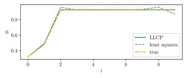
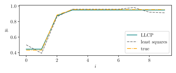
Figure 1: Sample predictions and true output.

Numerical example.

We consider a specific numerical example, with $N=100$ training pairs, $n=20$, and $m=10$. The inputs were chosen according to

$$x=\exp(\tilde{x}),\quad\tilde{x}\sim\mathcal{N}(0,I).$$

We generated true parameter values $A^{\star}\in{\mbox{\bf R}}^{m\times n}$ (with entries sampled from a normal distribution with zero mean and standard deviation $0.1$) and $c^{\star}\in{\mbox{\bf R}}^{m}_{++}$ (with entries set to the absolute value of samples from a standard normal). The outputs were generated by

$$y=\phi(x+\exp(v);A^{\star},c^{\star}),\quad v\sim\mathcal{N}(0,I).$$

We generated a held-out validation set of $50$ pairs, using the same true parameters.

We implemented the LLCP (3) in CVXPY, and used PyTorch and CVXPY Layers to train it using our gradient method. To initialize the parameters $A$ and $c$, we computed a least-squares monomial fit to the training data to obtain $A^{\mathrm{lstsq}}$ and $c^{\mathrm{lstsq}}$, via the method described in [Boy+07, §8.3]. From this initialization, we ran 10 iterations of our gradient method. Each iteration, which requires solving and differentiating through 150 LLCPs (100 for the training data, and 50 for logging the validation error), took roughly 10 seconds on a 2012 MacBook Pro with 16 GB of RAM and a 2.7 GHz Intel Core i7 processor.

The least-squares fit has a validation error of 0.014. The LLCP, with parameters $A=A^{\mathrm{lstsq}}$ and $c=c^{\mathrm{lstsq}}$, has a validation error of 0.0081, which is reduced to to 0.0077 after training. Figure 1 plots sample predictions of the LLCP and the least-squares fit on a validation input, as well as the true output. The LLCP’s prediction is monotonic, while the least squares prediction is not.

6 Acknowledgments

We thank Shane Barratt, who suggested using an optimization layer to regress on sorted vectors, and Steven Diamond and Guillermo Angeris, for helpful discussions related to data fitting and the derivative implementation. Akshay Agrawal is supported by a Stanford Graduate Fellowship.

References

- [Aba+16] Martín Abadi, Paul Barham, Jianmin Chen, Zhifeng Chen, Andy Davis, Jeffrey Dean, Matthieu Devin, Sanjay Ghemawat, Geoffrey Irving and Michael Isard “TensorFlow: A system for large-scale machine learning.” In OSDI 16, 2016, pp. 265–283
- [Agr+19] A. Agrawal, S. Barratt, S. Boyd, E. Busseti and W. Moursi “diffcp: differentiating through a cone program, version 1.0”, https://github.com/cvxgrp/diffcp, 2019
- [Agr+19a] Akshay Agrawal, Brandon Amos, Shane Barratt, Stephen Boyd, Steven Diamond and J Zico Kolter “Differentiable oonvex optimization layers” In Advances in Neural Information Processing Systems, 2019, pp. 9558–9570
- [Agr+19b] Akshay Agrawal, Shane Barratt, Stephen Boyd, Enzo Busseti and Walaa Moursi “Differentiating through a cone program” In Journal of Applied and Numerical Optimization 1.2, 2019, pp. 107–115
- [Agr+19c] Akshay Agrawal, Shane Barratt, Stephen Boyd and Bartolomeo Stellato “Learning convex optimization control policies” In arXiv, 2019 arXiv:1912.09529 [math.OC]
- [ADB19] Akshay Agrawal, Steven Diamond and Stephen Boyd “Disciplined geometric programming” In Optimization Letters 13.5 Springer Berlin Heidelberg, 2019, pp. 961–976
- [Agr+19d] Akshay Agrawal, Akshay Naresh Modi, Alexandre Passos, Allen Lavoie, Ashish Agarwal, Asim Shankar, Igor Ganichev, Josh Levenberg, Mingsheng Hong, Rajat Monga and Shanqing Cai “TensorFlow Eager: A multi-stage, Python-embedded DSL for machine learning” In Proceedings of the 2nd SysML Conference, 2019
- [Agr+18] Akshay Agrawal, Robin Verschueren, Steven Diamond and Stephen Boyd “A rewriting system for convex optimization problems” In Journal of Control and Decision 5.1 Taylor & Francis, 2018, pp. 42–60
- [AK17] B. Amos and Z. Kolter “OptNet: Differentiable optimization as a layer in neural networks” In International Conference on Machine Learning 70, 2017, pp. 136–145
- [Amo19] Brandon Amos “Differentiable optimization-based modeling for machine learning”, 2019
- [Amo+18] Brandon Amos, Ivan Jimenez, Jacob Sacks, Byron Boots and J. Zico Kolter “Differentiable MPC for end-to-end planning and control” In Advances in Neural Information Processing Systems, 2018, pp. 8299–8310
- [ApS19] MOSEK ApS “MOSEK optimization suite”, http://docs.mosek.com/9.0/intro.pdf, 2019
- [BB20] Shane Barratt and Stephen Boyd “Fitting a kalman smoother to data” To appear in Engineering Optimization In arXiv, 2020 arXiv:1910.08615 [math.OC]
- [BB20a] Shane Barratt and Stephen Boyd “Least squares auto-tuning” To appear in American Control Conference In arXiv, 2020 arXiv:1904.05460 [math.OC]
- [Bed+59] L. Beda, L. Korolev, N. Sukkikh and T. Frolova “Programs for automatic differentiation for the machine BESM”, 1959
- [Ber+20] Quentin Berthet, Mathieu Blondel, Olivier Teboul, Marco Cuturi, Jean-Philippe Vert and Francis Bach “Learning with differentiable perturbed optimizers” In arXiv, 2020 arXiv:2002.08676 [cs.LG]
- [BS00] J. Bonnans and A. Shapiro “Perturbation Analysis of Optimization Problems”, Springer Series in Operations Research Springer-Verlag, New York, 2000, pp. xviii+601 DOI: 10.1007/978-1-4612-1394-9
- [Boy+05] Stephen Boyd, Seung-Jean Kim, Dinesh Patil and Mark Horowitz “Digital circuit optimization via geometric programming” In Operations Research 53.6 Linthicum, Maryland, USA: INFORMS, 2005, pp. 899–932 DOI: 10.1287/opre.1050.0254
- [Boy+07] Stephen Boyd, Seung-Jean Kim, Lieven Vandenberghe and Arash Hassibi “A tutorial on geometric programming” In Optimization and Engineering 8.1 Springer, 2007, pp. 67
- [BV04] Stephen Boyd and Lieven Vandenberghe “Convex Optimization” New York, NY, USA: Cambridge University Press, 2004
- [BH18] Arthur Brown and Wesley Harris “A vehicle design and optimization model for on-demand aviation” In AIAA/ASCE/AHS/ASC Structures, Structural Dynamics, and Materials Conference, 2018
- [BDH20] Edward Burnell, Nicole Damen and Warren Hoburg “GPkit: A human-centered approach to convex optimization in engineering design” In Proceedings of the 2020 CHI Conference on Human Factors in Computing Systems, 2020
- [BMB19] Enzo Busseti, Walaa Moursi and Stephen Boyd “Solution refinement at regular points of conic problems” In Computational Optimization and Applications 74, 2019, pp. 627–643
- [CGP19] Giuseppe Calafiore, Stephane Gaubert and Corrado Possieri “Log-sum-exp neural networks and posynomial models for convex and log-log-convex data” In IEEE Transactions on Neural Networks and Learning Systems IEEE, 2019
- [Chi05] Mung Chiang “Geometric programming for communication systems” In Communications and Information Theory 2.1/2 Hanover, MA, USA: Now Publishers Inc., 2005, pp. 1–154 DOI: 10.1516/0100000005
- [CSB02] Mung Chiang, Arak Sutivong and Stephen Boyd “Efficient nonlinear optimizations of queuing systems” In Global Telecommunications Conference, 2002. GLOBECOM’02. IEEE 3, 2002, pp. 2425–2429 IEEE
- [Chi+07] Mung Chiang, Chee Wei Tan, Daniel Palomar, Daniel O’neill and David Julian “Power control by geometric programming” In IEEE Transactions on Wireless Communications 6.7 IEEE, 2007, pp. 2640–2651
- [Cla84] Richard Clasen “The solution of the chemical equilibrium programming problem with generalized Benders decomposition” In Operations Research 32.1, 1984, pp. 70–79
- [de ̵+18] Filipe de Avila Belbute-Peres, Kevin Smith, Kelsey Allen, Josh Tenenbaum and J. Zico Kolter “End-to-end differentiable physics for learning and control” In Advances in Neural Information Processing Systems, 2018, pp. 7178–7189
- [Dem82] Ron Dembo “Sensitivity analysis in geometric programming” In Journal of Optimization Theory and Applications 37.1, 1982, pp. 1–21
- [DB16] Steven Diamond and Stephen Boyd “CVXPY: A Python-embedded modeling language for convex optimization” In Journal of Machine Learning Research 17.83, 2016, pp. 1–5
- [DK77] John Dinkel and Gary Kochenberger “On sensitivity analysis in geometric programming” In Operations Research 25.1, 1977, pp. 155–163
- [DCB13] Alexander Domahidi, Eric Chu and Stephen Boyd “ECOS: An SOCP solver for embedded systems” In Control Conference (ECC), 2013 European, 2013, pp. 3071–3076 IEEE
- [DR09] Asen Dontchev and Ralph Tyrell Rockafellar “Implicit Functions and Solution Mappings” Springer, 2009
- [DPZ67] Richard Duffin, Elmor Peterson and Clarence Zener “Geometric Programming—Theory and Application” New York: Wiley, 1967
- [FM68] A. Fiacco and G. McCormick “Nonlinear Programming: Sequential Unconstrained Minimization Techniques” John WileySons, Inc., New York-London-Sydney, 1968, pp. xiv+210
- [Fia76] Anthony Fiacco “Sensitivity analysis for nonlinear programming using penalty methods” In Mathematical Programming 10.3, 1976, pp. 287–311
- [FJL18] R. Frostig, M. Johnson and C. Leary “Compiling machine learning programs via high-level tracing” In Systems for Machine Learning, 2018
- [FNB17] Anqi Fu, Balasubramanian Narasimhan and Stephen Boyd “CVXR: An R package for disciplined convex optimization” In arXiv, 2017 arXiv:1711.07582 [stat.CO]
- [GJF20] Zhenglin Geng, Daniel Johnson and Ronald Fedkiw “Coercing machine learning to output physically accurate results” In Journal of Computational Physics 406 Elsevier, 2020, pp. 109099
- [GHC19] Stephen Gould, Richard Hartley and Dylan Campbell “Deep declarative networks: A new hope” In arXiv, 2019 arXiv:1909.04866
- [GB14] Michael Grant and Stephen Boyd “CVX: MATLAB software for disciplined convex programming, version 2.1”, http://cvxr.com/cvx, 2014
- [GBY06] Michael Grant, Stephen Boyd and Yinyu Ye “Disciplined convex programming” In Global optimization Springer, 2006, pp. 155–210
- [GW08] A. Griewank and A. Walther “Evaluating Derivatives: Principles and Techniques of Algorithmic Differentiation” SIAM, 2008
- [HBL01] Maria Hershenson, Stephen Boyd and Thomas Lee “Optimal design of a CMOS op-amp via geometric programming” In IEEE Transactions on Computer-aided design of integrated circuits and systems 20.1 IEEE, 2001, pp. 1–21
- [HA14] Warren Hoburg and Pieter Abbeel “Geometric programming for aircraft design optimization” In AIAA Journal 52.11 American Institute of AeronauticsAstronautics, 2014, pp. 2414–2426
- [HKA16] Warren Hoburg, Philippe Kirschen and Pieter Abbeel “Data fitting with geometric-programming-compatible softmax functions” In Optimization and Engineering 17.4 Springer, 2016, pp. 897–918
- [Inn19] M. Innes “Don’t unroll adjoint: Differentiating SSA-form programs” In Advances in Neural Information Processing Systems, Workshop on Systems for ML and Open Source Software, 2019
- [KB02] S. Kandukuri and S. Boyd “Optimal power control in interference-limited fading wireless channels with outage-probability specifications” In Transactions on Wireless Communications 1.1 Piscataway, NJ, USA: IEEE Press, 2002, pp. 46–55 DOI: 10.1109/7693.975444
- [Ken53] David Kendall “Stochastic processes occurring in the theory of queues and their analysis by the method of the imbedded Markov chain” In The Annals of Mathematical Statistics JSTOR, 1953, pp. 338–354
- [Kyp90] Jerzy Kyparisis “Sensitivity analysis in geometric programming: Theory and computations” In Annals of Operations Research 27.1-4, 1990, pp. 39–63
- [Kyp88] Jerzy Kyparisis “Sensitivity analysis in posynomial geometric programming” In Journal of Optimization Theory and Applications 57.1, 1988, pp. 85–121
- [Li+04] Xin Li, Padmini Gopalakrishnan, Yang Xu and Lawrence Pileggi “Robust analog/RF circuit design with projection-based posynomial modeling” In Proceedings of the 2004 IEEE/ACM International Conference on Computer-aided Design, ICCAD ’04 Washington, DC, USA: IEEE Computer Society, 2004, pp. 855–862 DOI: 10.1109/ICCAD.2004.1382694
- [LFK18] Chun Ling, Fei Fang and J Zico Kolter “What game are we playing? End-to-end learning in normal and extensive form games” In Proceedings of the 27th International Joint Conference on Artificial Intelligence, 2018, pp. 396–402
- [Löf04] Johan Löfberg “YALMIP: A toolbox for modeling and optimization in MATLAB” In Proceedings of the CACSD Conference, 2004
- [O’D+16] Brendan O’Donoghue, Eric Chu, Neal Parikh and Stephen Boyd “Conic optimization via operator splitting and homogeneous self-dual embedding” In Journal of Optimization Theory and Applications 169.3 Springer, 2016, pp. 1042–1068
- [O’D+17] Brendan O’Donoghue, Eric Chu, Neal Parikh and Stephen Boyd “SCS: Splitting conic solver, version 2.1.0”, https://github.com/cvxgrp/scs, 2017
- [Ogu+19] Masaki Ogura, Junichi Harada, Masako Kishida and Ali Yassine “Resource optimization of product development projects with time-varying dependency structure” In Research in Engineering Design 30.3 Springer, 2019, pp. 435–452
- [OKL19] Masaki Ogura, Masako Kishida and James Lam “Geometric programming for optimal positive linear systems” In IEEE Transactions on Automatic Control IEEE, 2019
- [OP16] Masaki Ogura and Victor Preciado “Efficient containment of exact SIR Markovian processes on networks” In 2016 IEEE 55th Conference on Decision and Control (CDC), 2016, pp. 967–972 IEEE
- [Pas+19] Adam Paszke, Sam Gross, Francisco Massa, Adam Lerer, James Bradbury, Gregory Chanan, Trevor Killeen, Zeming Lin, Natalia Gimelshein and Luca Antiga “PyTorch: An imperative style, high-performance deep learning library” In Advances in Neural Information Processing Systems, 2019, pp. 8024–8035
- [Pre+14] Victor Preciado, Michael Zargham, Chinwendu Enyioha, Ali Jadbabaie and George Pappas “Optimal resource allocation for network protection: A geometric programming approach” In IEEE Transactions on Control of Network Systems 1.1, 2014, pp. 99–108
- [SBH18] Ali Saab, Edward Burnell and Warren Hoburg “Robust designs via geometric programming” In arXiv, 2018 arXiv:1808.07192 [math.OC]
- [Ude+14] Madeleine Udell, Karanveer Mohan, David Zeng, Jenny Hong, Steven Diamond and Stephen Boyd “Convex Optimization in Julia” In SC14 Workshop on High Performance Technical Computing in Dynamic Languages, 2014 arXiv:1410.4821 [math.OC]
- [XPB04] Yang Xu, Lawrence Pileggi and Stephen Boyd “ORACLE: Optimization with recourse of analog circuits including layout extraction” In Proceedings of the 41st Annual Design Automation Conference, DAC ’04 New York, NY, USA: ACM, 2004, pp. 151–154 DOI: 10.1145/996566.996611