Hamiltonian Monte Carlo using an adjoint- differentiated Laplace approximation: Bayesian inference for latent Gaussian models and beyond

Abstract

Gaussian latent variable models are a key class of Bayesian hierarchical models with applications in many fields. Performing Bayesian inference on such models can be challenging as Markov chain Monte Carlo algorithms struggle with the geometry of the resulting posterior distribution and can be prohibitively slow. An alternative is to use a Laplace approximation to marginalize out the latent Gaussian variables and then integrate out the remaining hyperparameters using dynamic Hamiltonian Monte Carlo, a gradient-based Markov chain Monte Carlo sampler. To implement this scheme efficiently, we derive a novel adjoint method that propagates the minimal information needed to construct the gradient of the approximate marginal likelihood. This strategy yields a scalable differentiation method that is orders of magnitude faster than state of the art differentiation techniques when the hyperparameters are high dimensional. We prototype the method in the probabilistic programming framework Stan and test the utility of the embedded Laplace approximation on several models, including one where the dimension of the hyperparameter is $\sim$6,000. Depending on the cases, the benefits can include an alleviation of the geometric pathologies that frustrate Hamiltonian Monte Carlo and a dramatic speed-up.

1 Introduction

Latent Gaussian models observe the following hierarchical structure:

$$\phi\sim\pi(\phi),\qquad\theta\sim\operatorname{\mathrm{Normal}}(0,K(\phi)),\qquad y\sim\pi(y\mid\theta,\phi).$$

Typically, single observations $y_{i}$ are independently distributed and only depend on a linear combination of the latent variables, that is $\pi(y_{i}\mid\theta,\phi)=\pi(y_{i}\mid a_{i}^{T}\theta,\phi)$, for some appropriately defined vectors $a_{i}$. This general framework finds a broad array of applications: Gaussian processes, spatial models, and multilevel regression models to name a few examples. We denote $\theta$ the latent Gaussian variable and $\phi$ the hyperparameter, although we note that in general $\phi$ may refer to any latent variable other than $\theta$. Note that there is no clear consensus in the literature on what constitutes a “latent Gaussian model”; we use the definition from the seminal work by Rue et al. [35].

We derive a method to perform Bayesian inference on latent Gaussian models, which scales when $\phi$ is high dimensional and can handle the case where $\pi(\phi\mid y)$ is multimodal, provided the energy barrier between the modes is not too strong. This scenario arises in, for example, general linear models with a regularized horseshoe prior [13] and in sparse kernel interaction models [1]. The main application for these models is studies with a low number of observations but a high-dimensional covariate, as seen in genomics.

The inference method we develop uses a gradient-based Markov chain Monte Carlo (MCMC) sampler, coupled with a Laplace approximation to marginalize out $\theta$. The key to successfully implementing this scheme is a novel adjoint method that efficiently differentiates the approximate marginal likelihood. In the case of a classic Gaussian process (Section 4), where $\mathrm{dim}(\phi)=2$, the computation required to evaluate and differentiate the marginal is on par with the GPstuff package [42], which uses the popular algorithm by Rasmussen and Williams [34]. The adjoint method is however orders of magnitude faster when $\phi$ is high dimensional. Figure 1 shows the superior scalability of the adjoint method on simulated data from a sparse kernel interaction model. We lay out the details of the algorithms and the experiment in Section 3.

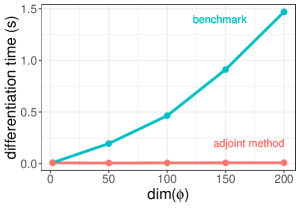
Figure 1: Wall time to differentiate the marginal density using the adjoint method (Algorithm 2) and, as a benchmark, the method by Rasmussen and Williams [34] (Algorithm 1).

1.1 Existing methods

Bayesian computation is, broadly speaking, split between two approaches: (i) MCMC methods that approximately sample from the posterior, and (ii) approximation methods in which one finds a tractable distribution that approximates the posterior (e.g. variational inference, expectation propagation, and asymptotic approximations). The same holds for latent Gaussian models, where we can consider (i) Hamiltonian Monte Carlo (HMC) sampling [31, 5] and (ii) approximation schemes such as variational inference (VI) [10] or marginalizing out the latent Gaussian variables with a Laplace approximation before deterministically integrating the hyperparameters [40, 35].

Hamiltonian Monte Carlo sampling.

When using MCMC sampling, the target distribution is

$$\pi(\theta,\phi\mid y)\propto\pi(y\mid\theta,\phi)\pi(\theta\mid\phi)\pi(\phi),$$

and the Markov chain explores the joint parameter space of $\theta$ and $\phi$.

HMC is a class of MCMC algorithms that powers many modern probabilistic programming languages, including Stan [12], PyMC3 [37], and TensorFlow Probability [16]. Its success is both empirically and theoretically motivated (e.g. [9]) and, amongst other things, lies in its ability to probe the geometry of the target distribution via the gradient. The algorithm is widely accessible through a combination of its dynamic variants [22, 5], which spare the users the cumbersome task of manually setting the algorithm’s tuning parameters, and automatic differentiation, which alleviates the burden of calculating gradients by hand (e.g. [27, 2, 21]). There are known challenges when applying HMC to hierarchical models, because of the posterior distribution’s problematic geometry [7]. In the case of latent Gaussian models, this geometric grief is often caused by the latent Gaussian variable, $\theta$, and its interaction with $\phi$. Certain samplers, such as Riemannian HMC [19, 4] and semi-separable HMC [46], are designed to better handle difficult geometries. While promising, these methods are difficult to implement, computationally expensive, and to our knowledge not widely used.

Variational inference.

VI proposes to approximate the target distribution, $\pi(\theta,\phi\mid y)$, with a tractable distribution, $q(\theta,\phi)$, which minimizes the Kullback-Leibler divergence between the approximation and the target. The optimization is performed over a pre-defined family of distributions, $\mathcal{Q}$. Adaptive versions, such as black-box VI [33] and automatic differentiation VI (ADVI) [25], make it easy to run the algorithm. VI is further made accessible by popular software libraries, including the above-mentioned probabilistic programming languages, and others packages such as GPyTorch for Gaussian processes [18]. For certain problems, VI is more scalable than MCMC, because it can be computationally much faster to solve an optimization problem than to generate a large number of samples. There are however known limitations with VI (e.g. [10, 45, 23, 15]). Of interest here is that $\mathcal{Q}$ may not include appropriate approximations of the target: mean field or full rank Gaussian families, for instance, will underestimate variance and settle on a single mode, even if the posterior is multimodal (e.g. [45]).

Marginalization using a Laplace approximation.

The embedded Laplace approximation is a popular algorithm, and a key component of the R packages INLA (integrated nested Laplace integration, [35, 36]) and TMB (template model builder, [24]), and the GPstuff package [42]. The idea is to marginalize out $\theta$ and then use standard inference techniques on $\phi$.

We perform the Laplace approximation

$$\pi(\theta\mid\phi,y)\approx\pi_{\mathcal{G}}(\theta\mid y,\phi):=\operatorname{\mathrm{Normal}}(\theta^{*},\Sigma^{*}),$$

where $\theta^{*}$ matches the mode and $[\Sigma^{*}]^{-1}$ the curvature of $\pi(\theta\mid\phi,y)$. Then, the marginal posterior distribution is approximated as follows:

$$\pi(\phi\mid y)\approx\pi_{\mathcal{G}}(\phi\mid y):=\pi(\phi)\frac{\pi(\theta^{*}\mid\phi)\pi(y\mid\theta^{*},\phi)}{\pi_{\mathcal{G}}(\theta^{*}\mid\phi,y)\pi(y)}.$$

Once we perform inference on $\phi$, we can recover $\theta$ using the conditional distribution $\pi_{\mathcal{G}}(\theta\mid\phi,y)$ and effectively marginalizing $\phi$ out. For certain models, this yields much faster inference than MCMC, while retaining comparable accuracy [35]. Furthermore the Laplace approximation as a marginalization scheme enjoys very good theoretical properties [40].

In the R package INLA, approximate inference is performed on $\phi$, by characterizing $\pi(\phi\mid y)$ around its presumed mode. This works well for many cases but presents two limitations: the posterior must be well characterized in the neighborhood of the estimated mode and it must be low dimensional, “2–5, not more than 20” [36]. In one of the examples we study, the posterior of $\phi$ is both high dimensional ($\sim$6000) and multimodal.

Hybrid methods.

Naturally we can use a more flexible inference method on $\phi$ such as a standard MCMC, as discussed by Gómez-Rubio and Rue [20], and HMC as proposed in GPstuff and TMB, the latter through its extension TMBStan and AdNuts (automatic differentiation with a No-U-Turn Sampler [29]). The target distribution of the HMC sampler is now $\pi_{\mathcal{G}}(\phi\mid y)$.

To use HMC, we require the gradient of $\log\pi_{\mathcal{G}}(y\mid\phi)$ with respect to $\phi$. Much care must be taken to ensure an efficient computation of this gradient. TMB and GPstuff exemplify two approaches to differentiate the approximate marginal density. The first uses automatic differentiation and the second adapts the algorithms in Rasmussen and Williams [34]. One of the main bottlenecks is differentiating the estimated mode, $\theta^{*}$. In theory, it is straightforward to apply automatic differentiation, by brute-force propagating derivatives through $\theta^{*}$, that is, sequentially differentiating the iterations of a numerical optimizer. But this approach, termed the direct method, is prohibitively expensive. A much faster alternative is to use the implicit function theorem (e.g. [3, 27]). Given any accurate numerical solver, we can always use the implicit function theorem to get derivatives, as notably done in the Stan Math Library [11] and in TMB’s inverse subset algorithm [24]. One side effect is that the numerical optimizer is treated as a black box. By contrast, Rasmussen and Williams [34] define a bespoke Newton method to compute $\theta^{*}$, meaning we can store relevant variables from the final Newton step when computing derivatives. In our experience, this leads to important computational savings. But overall this method is much less flexible, working well only when $\phi$ is low dimensional and requiring the user to pass the tensor of derivatives, $\partial K/\partial\phi$.

2 Aim and results of the paper

We improve the computation of HMC with an embedded Laplace approximation. Our implementation accommodates any covariance matrix $K$, without requiring the user to specify $\partial K/\partial\phi$, efficiently differentiates $\log\pi_{\mathcal{G}}(y\mid\phi)$, even when $\phi$ is high dimensional, and deploys dynamic HMC to perform inference on $\phi$. We introduce a novel adjoint method to differentiate $\log\pi_{\mathcal{G}}(y\mid\phi)$, build the algorithm in C++, and add it to the Stan language. Our approach combines the Newton solver of Rasmussen and Williams [34] with a non-trivial application of automatic differentiation.

Equipped with this implementation, we test dynamic HMC with an embedded Laplace approximation on a range of models, including ones with a high dimensional and multimodal hyperparameter. We do so by benchmarking our implementation against Stan’s dynamic HMC, which runs MCMC on both the hyperparameter and the latent Gaussian variable. For the rest of the paper, we call this standard use of dynamic HMC, full HMC. We refer to marginalizing out $\theta$ and using dynamic HMC on $\phi$, as the embedded Laplace approximation. Another candidate benchmark is Stan’s ADVI. Yao et al. [45] however report that ADVI underestimates the posterior variance and returns a unimodal approximation, even when the posterior is multimodal. We observe a similar behavior in the models we examine. For clarity, we relegate most of our analysis on ADVI to the Supplementary Material.

Our computer experiments identify cases where the benefits of the embedded Laplace approximation, as tested with our implementation, are substantial. In the case of a classic Gaussian process, with $\mathrm{dim}(\phi)=2$ and $\mathrm{dim}(\theta)=100$, we observe an important computational speed up, when compared to full HMC. We next study a general linear regression with a sparsity inducing prior; this time $\mathrm{dim}(\phi)\approx 6,000$ and $\mathrm{dim}(\theta)\approx 100$. Full HMC struggles with the posterior’s geometry, as indicated by divergent transitions, and requires a model reparameterization and extensive tuning of the sampler. On the other hand, the embedded Laplace approximation evades many of the geometric problems and solves the approximate problem efficiently. We observe similar results for a sparse kernel interaction model, which looks at second-order interactions between covariates [1]. Our results stand in contrast to the experiments presented in Monnahan and Kristensen [29], who used a different method to automatically differentiate the Laplace approximation and reported at best a minor speed up. We do however note that the authors investigated different models than the ones we study here.

In all the studied cases, the likelihood is log-concave. Combined with a Gaussian prior, log-concavity guarantees that $\pi(\theta\mid\phi,y)$ is unimodal. Detailed analysis on the error introduced by the Laplace approximation for log-concave likelihoods can be found in references (e.g. [26, 41, 14, 43]) and are consistent with the results from our computer experiments.

3 Implementation for probabilistic programming

In order to run HMC, we need a function that returns the approximate log density of the marginal likelihood, $\log\pi_{\mathcal{G}}(y\mid\phi)$, and its gradient with respect to $\phi$, $\nabla_{\phi}\log\pi_{\mathcal{G}}(y\mid\phi)$. The user specifies the observations, $y$, and a function to generate the covariance $K$, based on input covariates $x$ and the hyperparameters $\phi$. In the current prototype, the user picks the likelihood, $\pi(y\mid\theta,\phi)$, from a set of options: for example, a likelihood arising from a Bernoulli distribution with a logit link.

Standard implementations of the Laplace approximation use the algorithms in Rasmussen and Williams [34, chapter 3 and 5] to compute (i) the mode $\theta^{*}$ and $\log\pi_{\mathcal{G}}(y\mid\phi)$, using a Newton solver; (ii) the gradient $\nabla_{\phi}\log\pi_{\mathcal{G}}(y\mid\phi)$ (Algorithm 1), and (iii) simulations from $\pi_{\mathcal{G}}(\theta\mid y,\phi)$. The major contribution of this paper is to construct a new differentiation algorithm, i.e. item (ii).

3.1 Using automatic differentiation in the algorithm of Rasmussen and Williams [34]

The main difficulty with Algorithm 1 from Rasmussen and Williams [34] is the requirement for $\partial K/\partial\phi_{j}$ at line 8. For classic problems, where $K$ is, for instance, a exponentiated quadratic kernel, the derivatives are available analytically. This is not the case in general and, in line with the paradigm of probabilistic programming, we want a method that does not require the user to specify the tensor of derivatives, $\partial K/\partial\phi$.

Algorithm 1 Gradient of the approximate marginal density, $\pi_{\mathcal{G}}(y\mid\phi)$, with respect to the hyperparameters $\phi$, adapted from algorithm 5.1 by Rasmussen and Williams [34, chapter 5]. We store and reuse terms computed during the final Newton step, algorithm 3.1 in Rasmussen and Williams [34, chapter 3].

input: $y$, $\phi$, $\pi(y\mid\theta,\phi)$

2:saved input from the Newton solver: $\theta^{*}$, $K$, $W^{\frac{1}{2}}$, $L$, $a$

$Z=\frac{1}{2}a^{T}\theta^{*}+\log\pi(y\mid\theta^{*},\phi)-\sum\log(\mathrm{diag}(L))$

4:$R=W^{\frac{1}{2}}L^{T}\setminus(L\setminus W^{\frac{1}{2}})$

$C=L\setminus(W^{\frac{1}{2}}K)$

6:$s_{2}=-\frac{1}{2}\mathrm{diag}(\mathrm{diag}(K)-\mathrm{diag}(C^{T}C))\nabla_{\theta}^{3}\log\pi(y\mid\theta^{*},\phi)$

for $j=1$ … $\mathrm{dim}(\phi)$

8:      $K^{\prime}=\partial K/\partial\phi_{j}$

      $s_{1}=\frac{1}{2}a^{T}K^{\prime}a-\frac{1}{2}\mathrm{tr}(RK^{\prime})$

10:      $b=K^{\prime}\nabla_{\theta}\log\pi(y\mid\theta,\phi)$

      $s_{3}=b-KRb$

12:      $\frac{\partial}{\partial\phi_{j}}\pi(y\mid\phi)=s_{1}+s_{2}^{T}s_{3}$

end for

14:return $\nabla_{\phi}\log\pi_{\mathcal{G}}(y\mid\phi)$

Automatic differentiation allows us to numerically evaluate $\partial K/\partial\phi$ based on computer code to evaluate $K$. To do this, we introduce the map $\mathcal{K}$

$$\mathcal{K} : \mathbb{R}^{p}\to\mathbb{R}^{n(n+1)/2}$$

$$\phi\to K,$$

where $p$ is the dimension of $\phi$ and $n$ that of $\theta$. To obtain the full tensor of derivatives, we require either $p$ forward mode sweeps or $n(n+1)/2$ reverse mode sweeps. Given the scaling, we favor forward mode and this works well when $p$ is small. However, once $p$ becomes large, this approach is spectacularly inefficient.

3.2 Adjoint method to differentiate the approximate log marginal density

To evaluate the gradient of a composite map, it is actually not necessary to compute the full Jacobian matrix of intermediate operations. This is an important, if often overlooked, property of automatic differentiation and the driving principle behind adjoint methods (e.g. [17]). This idea motivates an algorithm that does not explicitly construct $\partial K/\partial\phi$, a calculation that is both expensive and superfluous. Indeed, it suffices to evaluate $w^{T}\partial K/\partial\phi$ for the correct cotangent vector, $w^{T}$, an operation we can do in a single reverse mode sweep of automatic differentiation.

Theorem 1

Let $\log\pi_{\mathcal{G}}(y\mid\phi)$ be the approximate log marginal density in the context of a latent Gaussian model. Let $a$ be defined as in the Newton solver by Rasmussen and Williams [34, chapter 3], and let $R$ and $s_{2}$ be defined as in Algorithm 1. Then

$$\nabla_{\phi}\log\pi_{\mathcal{G}}(y\mid\phi)=w^{T}\frac{\partial K}{\partial\phi},$$

where the gradient is with respect to $\phi$ and

$$w^{T}=\frac{1}{2}aa^{T}-\frac{1}{2}R+(s_{2}+RKs_{2})[\nabla_{\theta}\log\pi(y\mid\theta,\phi)]^{T}.$$

The proof follows from Algorithm 1 and noting that all the operations in $\partial K/\partial\phi_{j}$ are linear. We provide the details in the Supplementary Material. Armed with this result, we build Algorithm 2, a method that combines the insights of Rasmussen and Williams [34] with the principles of adjoint methods.

Algorithm 2 Gradient of the approximate marginal log density, $\log\pi_{\mathcal{G}}(y\mid\phi)$, with respect to the hyperparameters, $\phi$, using reverse mode automatic differentiation and theorem 1.

input: $y$, $\phi$, $\pi(y\mid\theta,\phi)$

2:Do lines 2 - 6 of Algorithm 1.

Initiate an expression graph for automatic differentiation with $\phi_{v}=\phi$.

4:$K_{v}=\mathcal{K}(\phi_{v})$

$w^{T}=\frac{1}{2}aa^{T}-\frac{1}{2}R+(s_{2}+RKs_{2})[\nabla_{\theta}\log\pi(y\mid\theta,\phi)]^{T}$

6:Do a reverse sweep over $K$, with $w^{T}$ as the initial cotangent to obtain $\nabla_{\phi}\log\pi_{\mathcal{G}}(y\mid\phi)$.

return: $\nabla_{\phi}\log\pi_{\mathcal{G}}(y\mid\phi)$.

Figure 1 shows the time required for one evaluation and differentiation of $\log\pi_{\mathcal{G}}(y\mid\phi)$ for the sparse kernel interaction model developed by Agrawal et al. [1] on simulated data. The covariance structure of this model is nontrivial and analytical derivatives are not easily available. We simulate a range of data sets for varying dimensions, $p$, of $\phi$. For low dimensions, the difference is small; however, for $p=200$, Algorithm 2 is more than 100 times faster than Algorithm 1, requiring 0.009 s, instead of 1.47 s.

4 Gaussian process with a Poisson likelihood

We fit the disease map of Finland by Vanhatalo et al. [41] which models the mortality count across the country. The data is aggregated in $n=911$ grid cells. We use 100 cells, which allows us to fit the model quickly both with full HMC and HMC using an embedded Laplace approximation. For the $i^{\mathrm{th}}$ region, we have a 2-dimensional coordinate $x_{i}$, the counts of deaths $y_{i}$, and the standardized expected number of deaths, $y_{e}^{i}$. The full latent Gaussian model is

$$(\rho,\alpha)\sim\pi(\rho,\alpha),\qquad\theta\sim\operatorname{\mathrm{Normal}}(0,K(\alpha,\rho,x)),\qquad y_{i}\sim\mathrm{Poisson}(y_{e}^{i}e^{\theta_{i}}),$$

where $K$ is an exponentiated quadratic kernel, $\alpha$ is the marginal standard deviation and $\rho$ the characteristic length scale. Hence $\phi=(\alpha,\rho)$.

Fitting this model with MCMC requires running the Markov chains over $\alpha$, $\rho$, and $\theta$. Because the data is sparse — one observation per group — the posterior has a funnel shape which can lead to biased MCMC estimates [30, 7]. A useful diagnostic for identifying posterior shapes that challenge the HMC sampler is divergent transitions, which occur when there is significant numerical error in the computation of the Markov chain trajectory [5].

To remedy these issues, we reparameterize the model and adjust the target acceptance rate, $\delta_{a}$. $\delta_{a}$ controls the precision of HMC, with the usual trade-off between accuracy and speed. For well behaved problems, the optimal value is 0.8 [8] but posteriors with highly varying curvature require a higher value. Moreover, multiple attempts at fitting the model must be done before we correctly tune the sampler and remove all the divergent transitions. See the Supplementary Material for more details.

An immediate benefit of the embedded Laplace approximation is that we marginalize out $\theta$ and only run HMC on $\alpha$ and $\rho$, a two-dimensional and typically well behaved parameter space. In the case of the disease map, we do not need to reparameterize the model, nor adjust $\delta_{a}$.

We fit the models with both methods, using 4 chains, each with 500 warmup and 500 sampling iterations. A look at the marginal distributions of $\alpha$, $\rho$, and the first two elements of $\theta$ suggests the posterior samples generated by full HMC and the embedded Laplace approximation are in close agreement (Figure 2). With a Poisson likelihood, the bias introduced by the Laplace approximation is small, as shown by Vanhatalo et al. [41]. We benchmark the Monte Carlo estimates of both methods against results from running 18,000 MCMC iterations. The embedded Laplace approximations yields comparable precision, when estimating expectation values, and is an order of magnitude faster (Figure 2). In addition, we do not need to tune the algorithm and the MCMC warmup time is much shorter ($\sim$10 seconds against $\sim$200 seconds for full HMC).

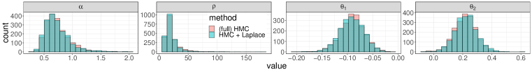
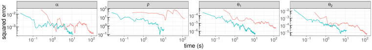
Figure 2: (Up) Posterior samples obtained with full HMC and the embedded Laplace approximation when fitting the disease map. (Down) Error when estimating the expectation value against wall time. Unreported in the figure is that we had to fit full HMC twice before obtaining good tuning parameters.

5 General linear regression model with a regularized horseshoe prior

Consider a regression model with $n$ observations and $p$ covariates. In the “$p\gg n$” regime, we typically need additional structure, such as sparsity, for accurate inference. The horseshoe prior [13] is a useful prior when it is assumed that only a small portion of the regression coefficients are non-zero. Here we use the regularized horseshoe prior by Piironen and Vehtari [32]. The horseshoe prior is parameterized by a global scale term, the scalar $\tau$, and local scale terms for each covariate, $\lambda_{j}$, $j=1,\ldots,p$. Consequently the number of hyperparameters is $\mathcal{O}(p)$.

To use the embedded Laplace approximation, we recast the regularized linear regression as a latent Gaussian model. The benefit of the approximation is not a significant speedup, rather an improved posterior geometry, due to marginalizing $\theta$ out. This means we do not need to reparameterize the model, nor fine tune the sampler. To see this, we examine the genetic microarray classification data set on prostate cancer used by Piironen and Vehtari [32] and fit a regression model with a Bernoulli distribution and a logit link. Here, $\mathrm{dim}(\theta)=102$ and $\mathrm{dim}(\phi)=5,966$.

We use 1,000 iterations to warm up the sampler and 12,000 sampling iterations. Tail quantiles, such as the $90^{\mathrm{th}}$ quantile, allow us to identify parameters which have a small local shrinkage and thence indicate relevant covariates. The large sample size is used to reduce the Monte Carlo error in our estimates of these extreme quantiles.

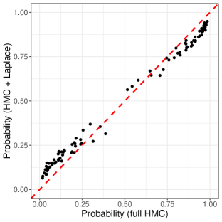
Figure 3: Expectation value for the probability of developing prostate cancer, as estimated by full HMC and HMC using an embedded Laplace approximation.

Fitting this model with full HMC requires a fair amount of work: the model must be reparameterized and the sampler carefully tuned, after multiple attempts at a fit. We use a non-centered parameterization, set $\delta_{a}=0.999$ (after attempting $\delta_{a}=0.8$ and $\delta_{a}=0.99$) and do some additional adjustments. Even then we obtain 13 divergent transitions over 12,000 sampling iterations. The Supplementary Material describes the tuning process in all its thorny details. By contrast, running the embedded Laplace approximation with Stan’s default tuning parameters produces 0 divergent transitions. Hence the approximate problem is efficiently solved by dynamic HMC. Running ADVI on this model is also straightforward.

Table 1 shows the covariates with the highest $90^{\mathrm{th}}$ quantiles, which are softly selected by full HMC, the embedded Laplace approximation and ADVI. For clarity, we exclude ADVI from the remaining figures but note that it generates, for this particular problem, strongly biased inference; more details can be found in the Supplementary Material. Figure 3 compares the expected probability of developing cancer. Figure 4 compares the posterior samples and the error when estimating various quantities of interest, namely (i) the expectation value of the global shrinkage, $\tau$, and the slab parameter, $c_{\mathrm{aux}}$; and (ii) the $90^{\mathrm{th}}$ quantile of two local shrinkage parameters. As a benchmark we use estimates obtained from 98,000 MCMC iterations.

Table 1: Top six covariate indices, $i$, with the highest $90^{\mathrm{th}}$ quantiles of $\log\lambda_{i}$ for the general linear model with a regularized horseshoe prior. The first two methods are in good agreement; ADVI selects different covariates, in part because it approximates the multimodal posterior with a unimodal distribution (see the Supplementary Material).

(full) HMC	2586	1816	4960	4238	4843	3381
HMC + Laplace	2586	1816	4960	4647	4238	3381
ADVI	1816	2416	4284	2586	5279	4940

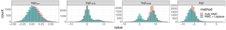
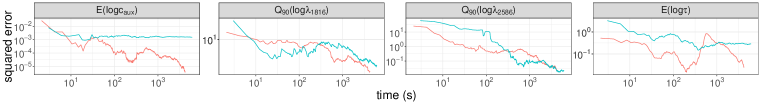
Figure 4: (Up) Posterior samples obtained with full HMC and HMC using an embedded Laplace approximation when fitting a general linear regression with a regularized horseshoe prior. (Down) Error when estimating various quantities of interest against wall time. $E$ stands for “expectation” and $Q_{90}$, “90^th quantile”. Unreported in the figure is that we had to run full HMC four times before obtaining reasonable tuning parameters.

The Laplace approximation yields slightly less extreme probabilities of developing cancer than the corresponding full model. This behavior is expected for latent Gaussian models with a Bernoulli observation model, and has been studied in the cases of Gaussian processes and Gaussian random Markov fields (e.g. [26, 14, 43]). While introducing a bias, the embedded Laplace approximation yields accuracy comparable to full HMC when evaluating quantities of interest.

6 Sparse kernel interaction model

A natural extension of the general linear model is to include interaction terms. To achieve better computational scalability, we can use the kernel interaction trick by Agrawal et al. [1] and build a sparse kernel interaction model (SKIM), which also uses the regularized horseshoe prior by Piironen and Vehtari [32]. The model is an explicit latent Gaussian model and uses a non-trivial covariance matrix. The full details of the model are given in the Supplementary Material.

When fitting the SKIM to the prostate cancer data, we encounter similar challenges as in the previous section: $\sim$150 divergent transitions with full HMC when using Stan’s default tuning parameters. The behavior when adding the embedded Laplace approximation is much better, although there are still $\sim$3 divergent transitions, which indicates that this problem remains quite difficult even after the approximate marginalization. We also find large differences in running time. The embedded Laplace approximation runs for $\sim$10 hours, while full HMC takes $\sim$20 hours with $\delta_{a}=0.8$ and $\sim$50 hours with $\delta_{a}=0.99$, making it difficult to tune the sampler and run our computer experiment.

Table 2: Top six covariate indices, $i$, with the highest $90^{\mathrm{th}}$ quantiles of $\log\lambda_{i}$ for the SKIM.

(full) HMC	2586	2660	2679	2581	2620	2651
HMC + Laplace	2586	2679	2660	2581	2620	2548
ADVI	2586	2526	2106	2550	2694	2166

For computational convenience, we fit the SKIM using only 200 covariates, indexed 2500 - 2700 to encompass the 2586^th covariate which we found to be strongly explanatory. This allows us to easily tune full HMC without altering the takeaways of the experiment. Note that the data here used is different from the data we used in the previous section (since we only examine a subset of the covariates) and the marginal posteriors should therefore not be compared directly.

As in the previous section, we generate 12,000 posterior draws for each method. For full HMC we obtain 36 divergent transitions with $\delta_{a}=0.8$ and 0 with $\delta_{a}=0.99$. The embedded Laplace approximation produces 0 divergences with $\delta_{a}=0.8$. Table 2 shows the covariates which are softly selected. As before, we see a good overlap between full HMC and the embedded Laplace approximation, and mostly disagreeing results from ADVI. Figure 5 compares (i) the posterior draws of full HMC and the embedded Laplace approximation, and (ii) the error over time, benchmarked against estimates from 98,000 MCMC iterations, for certain quantities of interest. We obtain comparable estimates but note that the Laplace approximation introduces a bias, which becomes more evident over longer runtimes.

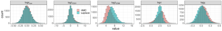
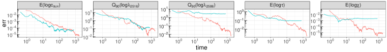
Figure 5: (Up) Samples obtained with full HMC and HMC using an embedded Laplace approximation when fitting the SKIM. (Down) Error when estimating various quantities of interest against wall time. $E$ stands for “expectation” and $Q_{90}$, “90^th quantile”. Unreported in the figure is that we had to run full HMC twice before obtaining reasonable tuning parameters.

7 Discussion

Equipped with a scalable and flexible differentiation algorithm, we expand the regime of models to which we can apply the embedded Laplace approximation. HMC allows us to perform inference even when $\phi$ is high dimensional and multimodal, provided the energy barrier is not too strong. In the case where $\mathrm{dim}(\theta)\gg\mathrm{dim}(\phi)$, the approximation also yields a dramatic speedup. When $\mathrm{dim}(\theta)\ll\mathrm{dim}(\phi)$, marginalizing $\theta$ out can still improve the geometry of the posterior, saving the user time otherwise spent tuning the sampling algorithm. However, when the posterior is well-behaved, the approximation may not provide any benefit.

Our next step is to further develop the prototype for Stan. We are also aiming to incorporate features that allow for a high performance implementation, as seen in the packages INLA, TMB, and GPstuff. Examples include support for sparse matrices required to fit latent Markov random fields, parallelization and GPU support.

We also want to improve the flexibility of the method by allowing users to specify their own likelihood. TMB provides this flexibility but in our view two important challenges persist. Recall that unlike full HMC, which only requires first-order derivatives, the embedded Laplace approximation requires the third-order derivative of the likelihood (but not of the other components in the model). It is in principle possible to apply automatic differentiation to evaluate higher-order derivatives and most libraries, including Stan, support this; but, along with feasibility, there is a question of efficiency and practicality (e.g. [6]): the automated evaluation of higher-order derivatives is often prohibitively expensive. The added flexibility also burdens us with more robustly diagnosing errors induced by the approximation. There is extensive literature on log-concave likelihoods but less so for general likelihoods. Future work will investigate diagnostics such as importance sampling [44], leave-one-out cross-validation [43], and simulation based calibration [39].

Broader Impact

Through its multidisciplinary nature, the here presented research can act as a bridge between various communities of statistics and machine learning. We hope practitioners of MCMC will consider the benefits of approximate distributions and vice-versa. This work may be a stepping stone to a broader conversation on how, what we have called the two broad approaches of Bayesian computation, can be combined. The paper also raises awareness about existing technologies and may dispel certain misconceptions. For example, our use of the adjoint principle shows that automatic differentiation is not a simple application of the chain rule, but quite a bit more clever than that.

Our goal is to make the method readily available to practitioners across multiple fields, which is why our C++ code and prototype Stan interface are open-source. While there is literature on the Laplace approximation, the error it introduces, and the settings in which it works best, we realize not all potential users will be familiar with it. To limit misuse, we must complement our work with pedagogical material built on the existing references, as well as support and develop more diagnostic tools.

Appendix (Supplementary Material)

We review the Newton solver proposed by Rasmussen and Williams [34] and prove theorem 1, the main result required to do build an adjoint method for the embedded Laplace approximation. We next present our prototype code and provide details for the models used in our computer experiments.

Appendix A Newton solver for the embedded Laplace approximation

Algorithm 3 Newton solver for the embedded Laplace approximation [34, chapter 3]

input: $K$, $y$, $\pi(y\mid\theta,\phi)$

2:$\theta^{*}=\theta_{0}$           (initialization)

repeat

4:      $W=-\nabla_{\theta}\nabla_{\theta}\log\pi(y\mid\theta^{*},\phi)$

      $L=\mathrm{Cholesky}(I+W^{\frac{1}{2}}KW^{\frac{1}{2}})$

6:      $b=W\theta^{*}+\nabla_{\theta}\log\pi(y\mid\theta^{*},\phi)$

      $a=b-W^{\frac{1}{2}}L^{T}\setminus(L\setminus(W^{\frac{1}{2}}Kb))$

8:      $\theta^{*}=Ka$

until convergence

10:$\log\pi(y\mid\phi)=-\frac{1}{2}a^{T}\theta^{*}+\log\pi(y\mid\theta^{*},\phi)-\sum_{i}\log L_{ii}$

return: $\theta^{*}$, $\log\pi_{\mathcal{G}}(y\mid\phi)$

Algorithm 3 is a transcription of the Newton method by Rasmussen and Williams [34, chapter 3] using our notation. As a convergence criterion, we use the change in the objective function between two iterations

$$\Delta\log\pi(\theta\mid y,\phi)\leq\epsilon$$

for a specified $\epsilon$. This is consistent with the approach used in GPStuff [42]. We store the following variables generated during the final Newton step to use them again when computing the gradient: $\theta^{*}$, $K$, $W^{\frac{1}{2}}$, $L$, and $a$. This avoids redundant computation and spares us an expensive Cholesky decomposition.

Appendix B Building the adjoint method

To compute the gradient of the approximate log marginal with respect to $\phi$, $\nabla\log\pi_{\mathcal{G}}(y\mid\phi)$, we exploit several important principles of automatic differentiation. While widely used in statistics and machine learning, these principles remain arcane to many practitioners and deserve a brief review. We will then construct the adjoint method (theorem 1 and algorithm 2) as a correction to algorithm 1.

B.1 Automatic differentiation

Given a composite map

$$f=f^{L}\circ f^{L-1}\circ...f^{1},$$

the chain rule teaches us that the corresponding Jacobian matrix observes a similar decomposition:

$$J=J_{L}\cdot J_{L-1}\cdot...\cdot J_{1}.$$

Based on computer code to calculate $f$, a forward mode sweep automatic differentiation numerically evaluates the action of the Jacobian matrix on the initial tangent $u$, or directional derivative $J\cdot u$. Extrapolating from the chain rule

$$\begin{aligned} J\cdot u&=J_{L}\cdot J_{L-1}\cdot...\cdot J_{3}\cdot J_{2}\cdot J_{1}\cdot u\\ &=J_{L}\cdot J_{L-1}\cdot...\cdot J_{3}\cdot J_{2}\cdot u_{1}\\ &=J_{L}\cdot J_{L-1}\cdot...\cdot J_{3}\cdot u_{2}\\ &...\\ &=J_{L}\cdot u_{L-1},\\ \end{aligned}$$

where the $u_{l}$’s verify the recursion relationship

$$\begin{aligned} u_{1}&=J_{1}\cdot u,\\ u_{l}&=J_{l}\cdot u_{l-1}.\\ \end{aligned}$$

If our computation follows the steps outlined above we never need to explicitly compute the full Jacobian matrix, $J_{l}$, of an intermediate function, $f^{l}$; rather we only calculate a sequence of Jacobian-tangent products. Similarly a reverse mode sweep evaluates the contraction of the Jacobian matrix with a cotangent, $w^{T}$, yielding $w^{T}J$, by computing a sequence cotangent-Jacobian products.

Hence, in the case of the embedded Laplace approximation, where

$$\mathcal{K}: \phi \to K$$

$$\mathbb{R}^{p} \to\mathbb{R}^{(n+1)n/2}$$

is an intermediate function, we do not need to explicitly compute $\partial K/\partial\phi$ but only $w^{T}\partial K/\partial\phi$ for the appropriate cotangent vector. This type of reasoning plays a key role when differentiating functionals of implicit functions – for example, probability densities that depend on solutions to ordinary differential equations – and leads to so-called adjoint methods [e.g. 17].

B.2 Derivation of the adjoint method

In this section we provide a proof of theorem 1. As a starting point, assume algorithm 1 is valid. The proof can be found in Rasmussen and Williams [34, chapter 5]. The key observation is that all operations performed on

$$\frac{\partial K}{\partial\phi_{j}}$$

are linear. Algorithm 1 produces a map

$$\mathcal{Z} :\partial K/\partial\phi_{j} \to\frac{\partial}{\partial\phi_{j}}\pi(y\mid\phi)$$

$$:\mathbb{R}^{n\times n} \to\mathbb{R},$$

and constructs the gradient one element at a time. By linearity,

$$\frac{\partial}{\partial\phi_{j}}\mathcal{Z}(K)=\mathcal{Z}\left(\frac{\partial K}{\partial\phi_{j}}\right).$$

Thus an alternative approach to compute the gradient is to calculate the scalar $\mathcal{Z}(K)$ and then use a single reverse mode sweep of automatic differentiation, noting that $\mathcal{Z}$ is an analytical function. This produces Algorithm 4.

Algorithm 4 Gradient of the approximate marginal log density, $\log\pi_{\mathcal{G}}(y\mid\phi)$, with respect to the hyperparameters, $\phi$, using reverse mode automatic differentiation

input: $y$, $\phi$, $\pi(y\mid\theta,\phi)$

2:Do lines 2 - 6 of Algorithm 2.

Initiate an expression tree for automatic differentiation with $\phi_{v}=\phi$.

4:$K_{v}=\mathcal{K}(\phi_{v})$

$z=\mathcal{Z}(K_{v})$

6:Do a reverse-sweep over $z$ to obtain $\nabla_{\phi}\log\pi(y\mid\phi)$.

return: $\nabla_{\phi}\log\pi(y\mid\phi)$.

At this point, the most important is done in order to achieve scalability: we no longer explicitly compute $\partial K/\partial\phi$ and are using a single reverse mode sweep.

Automatic differentiation, for all its relatively cheap cost, still incurs some overhead cost. Hence, where possible, we still want to use analytical results to compute derivatives. In particular, we can analytically work out the cotangent

$$w^{T}:=\frac{\partial z}{\partial K}.$$

For the following calculations, we use a lower case, $k_{ij}$ and $r_{ij}$, to denote the $(ij)^{\mathrm{th}}$ element respectively of the matrices $K$ and $R$.

Consider

$$\mathcal{Z}(K)=s_{1}+s_{2}^{T}s_{3},$$

where, unlike in Algorithm 1, $s_{1}$ and $s_{3}$ are now computed using $K$, not $\partial K/\partial\phi_{j}$. We have

$$s_{1}=\frac{1}{2}a^{T}Ka-\frac{1}{2}\mathrm{tr}(RK).$$

Then

$$\frac{\partial}{\partial k_{i^{\prime}j^{\prime}}}a^{T}Ka=\frac{\partial}{\partial k_{i^{\prime}j^{\prime}}}\sum_{i}\sum_{j}a_{i}k_{ij}a_{j}=a_{i^{\prime}}a_{j^{\prime}},$$

and

$$\frac{\partial}{\partial k_{i^{\prime}j^{\prime}}}\mathrm{tr}(RK)=\frac{\partial}{\partial k_{i^{\prime}j^{\prime}}}\sum_{l}r_{il}k_{li}=r_{j^{\prime}i^{\prime}}.$$

Thus

$$\frac{\partial s_{1}}{\partial K}=\frac{1}{2}aa^{T}-\frac{1}{2}R^{T}.$$

For convenience, denote $l=\nabla_{\theta}\log\pi(y\mid\theta,\phi)$. We then have

$$\begin{aligned} b&=Kl,\\ s_{3}&=b-\tilde{K}Rb=(I-\tilde{K}R)b,\end{aligned}$$

where $\tilde{K}=K$, but is maintained fixed, meaning we do not propagate derivatives through it. Let $\tilde{A}=I-\tilde{K}R$ and let $\tilde{a}_{ij}$ denote the $(i,j)^{\mathrm{th}}$ element of $\tilde{A}$. Then

$$s_{2}^{T}s_{3}=\sum_{i}(s_{2})_{i}\left(\sum_{j}\tilde{a}_{ij}\sum_{m}k_{jm}l_{m}\right).$$

Thus

$$\frac{\partial}{\partial k_{i^{\prime}j^{\prime}}}s_{2}^{T}s_{3}=\sum_{i}(s_{2})_{i}\tilde{a}_{ii^{\prime}}l_{j^{\prime}}=l_{j^{\prime}}\sum_{i}(s_{2})_{i}\tilde{a}_{ii^{\prime}},$$

where the sum term is the $(i^{\prime})^{\mathrm{th}}$ element of $\tilde{A}s_{2}$. The above expression then becomes

$$\frac{\partial}{\partial K}s^{T}_{2}s_{3}=\tilde{A}s_{2}l^{T}=s_{2}l^{T}-KRs_{2}l^{T}.$$

Combining the derivative for $s_{1}$ and $s^{T}_{2}s_{3}$ we obtain

$$w^{T}=\frac{1}{2}aa^{T}-\frac{1}{2}R+(s_{2}+RKs_{2})[\nabla_{\theta}\log\pi(y\mid\theta,\phi)]^{T},$$

as prescribed by Theorem 1. This result is general, in the sense that it applies to any covariance matrix, $K$, and likelihood, $\pi(y\mid\theta,\phi)$. Our preliminary experiments, on the SKIM, found that incorporating the analytical cotangent, $w^{T}\!$, approximately doubles the differentiation speed.

Appendix C Computer code

The code used in this work is open source and detailed in this section.

C.1 Prototype Stan code

The Stan language allows users to specify the joint log density of their model. This is done by incrementing the variable target. We add a suite of functions, which return the approximate log marginal density, $\log\pi_{\mathcal{G}}(y\mid\phi)$. Hence, the user can specify the log joint distribution by incrementing target with $\log\pi_{\mathcal{G}}(y\mid\phi)$ and the prior $\log\pi(\phi)$. A call to the approximate marginal density looks as follows:

⬇

target +=

laplace_marginal_*_lpmf (y | n, K, phi, x, delta,

delta_int, theta0);

The * specifies the obervation model, typically a distribution and a link function, for example bernoulli_logit or poisson_log. The suffix lpmf is used in Stan to denote a log posterior mass function. y and n are sufficient statistics for the latent Gaussian variable, $\theta$; K is a function that takes in arguments phi, x, delta, and delta_int and returns the covariance matrix; and theta0 is the initial guess for the Newton solver, which seeks the mode of $\pi(\theta\mid\phi,y)$. Moreover, we have

• y: a vector containing the sum of counts/successes for each element of $\theta$,

• n: a vector with the number of observation for each element of $\theta$,

• K: a function defined in the functions block, with the signature (vector, data matrix, data real[], data int[]) ==> matrix. Note that only the first argument may be used to pass variables which depend on model parameters, and through which we propagate derivatives. The term data means an argument may not depend on model parameters.

• phi: the vector of hyperparameters,

• x: a matrix of data. For Gaussian processes, this is the coordinates, and for the general linear regression, the design matrix,

• delta: additional real data,

• delta_int: additional integer data,

• theta0: a vector of initial guess for the Newton solver.

It is also possible to specify the tolerance of the Newton solver. This structure is consistent with other higher-order functions in Stan, such as the algebraic solver and the ordinary differential equation solvers. It gives users flexibility when specifying $K$, but we recognize it is cumbersome. One item on our to-do list is to use variadic arguments, which remove the constraints on the signature of K, and allows users to pass any combination of arguments to K through laplace_marignal_*_lpmf.

For each observation model, we implement a corresponding random number generating function, with a call

⬇

theta = laplace_marginal_*_rng (y, n, K, phi, x, delta,

delta_int, theta0);

This generates a random sample from $\pi_{\mathcal{G}}(\theta\mid y,\phi)$. This function can be used in the generated quantities blocks and is called only once per iteration – in contrast with the target function which is called and differentiated once per integration step of HMC. Moreover the cost of generating $\theta$ is negligible next to the cost evaluating and differentiating $\log\pi(y\mid\phi)$ multiple times per iteration.

The interested reader may find a notebook with demo code, including R scripts and Stan files, at https://github.com/charlesm93/StanCon2020, as part of the 2020 Stan Conference [28].

C.2 C++ code

We incorporate the Laplace suite of functions inside the Stan-math library, a C++ library for automatic differentiation [11]. The library is open source and available on GitHub, https://github.com/stan-dev/math. Our most recent prototype exists on the branch try-laplace_approximation2. The code is structured around a main function

⬇

laplace_approximation (likelihood, K_functor, phi, x, delta,

delta_int, theta0);

with

• likelihood: a class constructed using y and n, which returns the log density, as well as its first, second, and third order derivatives.

• K_functor: a functor that computes the covariance matrix, $K$

• …: the remaining arguments are as previously described.

A user can specify a new likelihood by creating the corresponding class, meaning the C++ code is expandable.

To expose the code to the Stan language, we use Stan’s new OCaml transpiler, stanc3, https://github.com/stan-dev/stanc3 and again the branch try-laplace_approximation2.

Important note: the code is prototypical and currently not merged into Stan’s release or development branch.

C.3 Code for the computer experiment

The code is available on the GitHub public repository, https://github.com/charlems93/laplace_manuscript.

We make use of two new prototype packages: CmdStanR (https://mc-stan.org/cmdstanr/) and posterior (https://github.com/jgabry/posterior).

Appendix D Tuning dynamic Hamiltonian Monte Carlo

In this article, we use the dynamic Hamiltonian Monte Carlo sampler described by Betancourt [5] and implemented in Stan. This algorithm builds on the No-U Turn Sampler by Hoffman and Gelman [22], which adaptively tunes the sampler during a warmup phase. Hence for most problems, the user does not need to worry about tuning parameters. However, the models presented in this article are challenging and the sampler requires careful tuning, if we do not use the embedded Laplace approximation.

The main parameter we tweak is the target acceptance rate, $\delta_{a}$. To run HMC, we need to numerically compute physical trajectories across the parameter space by solving the system of differential equations prescribed by Hamilton’s equations of motion. We do this using a numerical integrator. A small step size, $\delta$, makes the integrator more precise but generates smaller trajectories, which leads to a less efficient exploration of the parameter space. When we introduce too much numerical error, the proposed trajectory is rejected. Adapt delta, $\delta_{a}\in(0,1)$, sets the target acceptance rate of proposed trajectories. During the warmup, the sampler adjusts $\delta$ to meet this target. For well-behaved problems, the optimal value of $\delta_{a}$ is 0.8 [8].

It should be noted that the algorithm does not necessarily achieve the target set by $\delta_{a}$ during the warmup. One approach to remedy this issue is to extend the warmup phase; specifically the final fast adaptation interval or term buffer [see 22, 38]. By default, the term buffer runs for 50 iterations (when running a warmup for 1,000 iterations). Still, making the term buffer longer does not guarantee the sampler attains the target $\delta_{a}$. There exist other ways of tuning the algorithm, but at this points, the technical burden on the user is already significant. What is more, probing how well the tuning parameters work usually requires running the model for many iterations.

Appendix E Automatic differentiation variational inference

ADVI automatically derives a variational inference algorithm, based on a user specified log joint density. Hence we can use the same Stan file we used for full HMC and, with the appropriate call, run ADVI instead of MCMC. The idea behind ADVI is to approximate the posterior over the unconstrained space using a Gaussian distribution, either with a diagonal covariance matrix – leading to a mean-field approximation – or with a full rank covariance matrix. The details of this procedure are described in [25]. Compared to full HMC, ADVI can be much faster, but in general it is difficult to assess how well the variational approximation describes the target posterior distribution without using an expensive benchmark [45, 23]. Furthermore, it can be challenging to assess the convergence of ADVI [15].

To run ADVI, we use the Stan file with which we ran full HMC. We depart from the default tuning parameters by decreasing the learning rate $\eta$ to 0.1, adjusting the tolerance, rel_tol_obj, and increasing the maximum number of iterations to 100,000. Our goal is to improve the accuracy of the optimizer as much as possible, while insuring that convergence is reached.

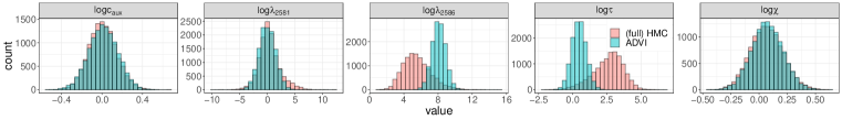
Figure 8: Samples obtained with full HMC and sampling from the variational approximation produced by ADVI when fitting the SKIM.

We compare the samples drawn from the variational approximation to samples drawn from full HMC in Figures 6, 7 and 8. For the studied examples, we find the approximation to be not very satisfactory, either because it underestimates the posterior variance, does not capture the skewness of the posterior distribution, or returns a unimodal approximation when in fact the posterior density is multimodal. These are all features which cannot be captured by a Gaussian over the unconstrained scale. Naturally, a different choice for $\mathcal{Q}$ could lead to better inference. Using a custom VI algorithm is however challenging, as we need to derive a useful variational family and hand-code the inference algorithm, rather than rely on the implementation in a probabilistic programming language.

Appendix F Model details

We review the models used in our computer experiments and point the readers to the relevant references.

F.1 Disease map

The disease map uses a Gaussian process with an exponentiated squared kernel,

$$k(x_{i},x_{j})=\alpha^{2}\exp\left(-\frac{(x_{i}-x_{j})^{T}(x_{i}-x_{j})}{\rho^{2}}\right).$$

The full latent Gaussian model is

$$\rho \sim \mathrm{invGamma}(a_{\rho},b_{\rho}),$$

$$\alpha \sim \mathrm{invGamma}(a_{\alpha},b_{\alpha}),$$

$$\theta \sim \operatorname{\mathrm{Normal}}(0,K(\alpha,\rho,x)),$$

$$y_{i} \sim \mathrm{Poisson}(y_{e}^{i}e^{\theta_{i}}),$$

where we put an inverse-Gamma prior on $\rho$ and $\alpha$.

When using full HMC, we construct a Markov chain over the joint parameter space $(\alpha,\rho,\theta)$. To avoid Neal’s infamous funnel [30] and improve the geometry of the posterior distribution, it is possible to use a non-centered parameterization:

$$(\rho,\alpha) \sim \pi(\rho,\alpha),$$

$$z \sim \operatorname{\mathrm{Normal}}(0,I_{n\times n}),$$

$$L = \mathrm{Cholesky\ decompose}(K),$$

$$\theta = Lz,$$

$$y_{i} \sim \mathrm{Poisson}(y^{i}_{e}e^{\theta_{i}}).$$

The Markov chain now explores the joint space of $(\alpha,\rho,z)$ and the $\theta$’s are generated by transforming the $z$’s. With the embedded Laplace approximation, the Markov chain only explores the joint space $(\alpha,\rho)$.

To run ADVI, we use the same Stan file as for full HMC and set tol_rel_obj to 0.005.

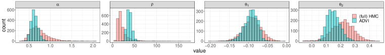
Figure 6: Samples obtained with full HMC and sampling from the variational approximation produced by ADVI when fitting the disease map. Unlike the embedded Laplace approximation, ADVI strongly disagrees with full HMC.

F.2 Regularized horseshoe prior

The horseshoe prior [13] is a sparsity inducing prior that introduces a global shrinkage parameter, $\tau$, and a local shrinkage parameter, $\lambda_{i}$ for each covariate slope, $\beta_{i}$. This prior operates a soft variable selection, effectively favoring $\beta_{i}\approx 0$ or $\beta_{i}\approx\hat{\beta}_{i}$, where $\hat{\beta}_{i}$ is the maximum likelihood estimator. Piironen and Vehtari [32] add another prior to regularize unshrunk $\beta$s, $\operatorname{\mathrm{Normal}}(0,c^{2})$, effectively operating a “soft-truncation” of the extreme tails.

F.2.1 Details on the prior

For computational stability, the model is parameterized using $c_{\mathrm{aux}}$, rather than $c$, where

$$c=s_{\mathrm{slab}}\sqrt{c_{\mathrm{aux}}}$$

with $s_{\mathrm{slab}}$ the slab scale. The hyperparameter is $\phi=(\tau,c_{\mathrm{aux}},\lambda)$ and the prior

$$\lambda_{i} \sim \mathrm{Student}_{t}(\nu_{\mathrm{local}},0,1),$$

$$\tau \sim \mathrm{Student}_{t}(\nu_{\mathrm{global}},0,s_{\mathrm{global}}),$$

$$c_{\mathrm{aux}} \sim \mathrm{inv}\Gamma(s_{\mathrm{df}}/2,s_{\mathrm{df}}/2),$$

$$\beta_{0} \sim \operatorname{\mathrm{Normal}}(0,c_{0}^{2}).$$

The prior on $\lambda$ independently applies to each element, $\lambda_{i}$.

Following the recommendation by Piironen and Vehtari [32], we set the variables of the priors as follows. Let $p$ be the number of covariates and $n$ the number of observations. Additionally, let $p_{0}$ be the expected number of relevant covariates – note this number does not strictly enforce the number of unregularized $\beta$s, because the priors have heavy enough tails that we can depart from $p_{0}$. For the prostate data, we set $p_{0}=5$. Then

$$s_{\mathrm{global}} = \frac{p_{0}}{\sqrt{n}(p-p_{0})},$$

$$\nu_{\mathrm{local}} = 1,$$

$$\nu_{\mathrm{global}} = 1,$$

$$s_{\mathrm{slab}} = 2,$$

$$s_{\mathrm{df}} = 100,$$

$$c_{0} = 5.$$

Next we construct the prior on $\beta$,

$$\beta_{i}\sim\operatorname{\mathrm{Normal}}(0,\tau^{2}\tilde{\lambda}_{i}^{2}),$$

where

$$\tilde{\lambda}_{i}^{2}=\frac{c^{2}\lambda_{i}^{2}}{c^{2}+\tau^{2}\lambda_{i}^{2}}.$$

F.2.2 Formulations of the data generating process

The data generating process is

$$\phi \sim \pi(\phi),$$

$$\beta_{0} \sim \operatorname{\mathrm{Normal}}(0,c_{0}^{2}),$$

$$\beta \sim \operatorname{\mathrm{Normal}}(0,\Sigma(\phi)),$$

$$y \sim \mathrm{Bernoulli\_logit}(\beta_{0}+X\beta),$$

or, equivalently,

$$\phi \sim \pi(\phi),$$

$$\theta \sim \operatorname{\mathrm{Normal}}(0,\,c_{0}^{2}I_{n\times n}+X\Sigma(\phi)X^{T}),$$

$$y \sim \mathrm{Bernoulli\_logit}(\theta).$$

For full HMC, we use a non-centered parameterization of the first formulation, much like we did for the disease map. The embedded Laplace approximation, as currently implemented, requires the second formulation, which is mathematically more convenient but comes at the cost of evaluating and differentiating $K=c^{2}I_{n\times n}+X\Sigma(\phi)X^{T}$. In this scenario, the main benefit of the Laplace approximation is not an immediate speed-up but an improved posterior geometry, due to marginalizing $\theta$ (and thus implicitly $\beta$ and $\beta_{0}$) out. This means we do not need to fine tune the sampler.

F.2.3 Fitting the model with full HMC

This section describes how to tune full HMC to fit the model at hand. Some of the details may be cumbersome to the reader. But the takeaway is simple: tuning the algorithm is hard and can be a real burden for the modeler.

Using a non-centered parameterization and with Stan’s default parameters, we obtain $\sim$150 divergent transitions. We increase the target acceptance rate to $\delta_{a}=0.99$ but find the sampler now produces 186 divergent transitions. A closer inspection reveals the divergences all come from a single chain, which also has a larger adapted step size, $\delta$. The problematic chain also fails to achieve the target acceptance rate. These results are shown in Table 3. From this, it seems increasing $\delta_{a}$ yet again may not provide any benefits. Instead we increase the term buffer from 50 iterations to 350 iterations. With this setup, we however obtain divergent transitions across all chains.

Table 3: Adapted tuning parameters across 4 Markov chains with $\delta_{a}=0.99$.

Chain	Step size	Acceptance rate	Divergences
1	0.0065	0.99	0
2	0.0084	0.90	186
3	0.0052	0.99	0
4	0.0061	0.99	0

This outcome indicates the chains are relatively unstable and emphasizes how difficult it is, for this type of model and data, to come up with the right tuning parameters. With $\delta_{a}=0.999$ and the extended term buffer we observe 13 divergent transitions. It is possible this result is the product of luck, rather than better tuning parameters. To be clear, we do not claim we found the optimal model parameterization and tuning parameters. There is however, to our knowledge, no straightforward way to do so.

F.2.4 Fitting the model with the embedded Laplace approximation

Running the algorithm with Stan’s default tuning parameters produces 0 divergent transitions over 12,000 sampling iterations.

F.2.5 Fitting the model with ADVI

To run ADVI, we use the same Stan file as for full HMC and set tol_rel_obj to 0.005.

The family of distribution, $\mathcal{Q}$, over which ADVI optimizes requires the exact posterior distribution to be unimodal over the unconstrained scale. This is a crucial limitation in the studied example, as shown in Figure 7. This notably affects our ability to select relevant covariates using the $90^{\mathrm{th}}$ posterior quantile. When examining the top six selected covariates (Table 1 in the main text), we find the result from ADVI to be in disagreement with full HMC and the embedded Laplace approximation. In particular, $\lambda_{2586}$ which corresponds, according to our other inference methods, to the most relevant covariate, has a relatively low $90^{\mathrm{th}}$ quantile. This is because ADVI only approximates the smaller mode of $\pi(\lambda_{2586}\mid y)$. Our results are consistent with the work by Yao et al. [45], who examine ADVI on a similar problem.

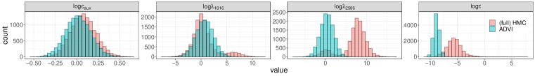
Figure 7: Samples obtained with full HMC and sampling from the variational approximation produced by ADVI when fitting a general linear model with a regularized horseshoe prior.

F.3 Sparse kernel interaction model

SKIM, developed by Agrawal et al. [1], extends the model of Piironen and Vehtari [32] by accounting for pairwise interaction effects between covariates. The generative model shown below uses the notation in F.2 instead of that in Appendix D of Agrawal et al. [1]:

$$\begin{split}\chi&\sim\mathrm{inv}\Gamma(s_{\mathrm{df}}/2,s_{\mathrm{df}}/2),\\ \eta_{2}&=\frac{\tau^{2}}{c^{2}}\chi,\\ \beta_{i}\mid\tau,\tilde{\lambda}&\sim\operatorname{\mathrm{Normal}}(0,\tau^{2}\tilde{\lambda}_{i}^{2}),\\ \beta_{j}\mid\tau,\tilde{\lambda}&\sim\operatorname{\mathrm{Normal}}(0,\tau^{2}\tilde{\lambda}_{i}^{2}),\\ \beta_{ij}\mid\eta_{2},\tilde{\lambda}&\sim\operatorname{\mathrm{Normal}}(0,\eta_{2}^{2}\tilde{\lambda}_{i}^{2}\tilde{\lambda}_{j}^{2}),\\ \beta_{0}\mid c_{0}^{2}&\sim\operatorname{\mathrm{Normal}}(0,c_{0}^{2}),\end{split}$$

where $\beta_{i}$ and $\beta_{ij}$ are the main and pairwise effects for covariates $x_{i}$ and $x_{i}x_{j}$, respectively, and $\tau$, $\tilde{\lambda}$, $c_{0}$ are defined in F.2.

Instead of sampling $\{\beta_{i}\}_{i=1}^{p}$ and $\{\beta_{ij}\}_{i,j=1}^{p}$, which takes at least $O(p^{2})$ time per iteration to store and compute, Agrawal et al. [1] marginalize out all the regression coefficients, only sampling $(\tau,\xi,\tilde{\lambda})$ via MCMC. Through a kernel trick and a Gaussian process re-parameterization of the model, this marginalization takes $O(p)$ time instead of $O(p^{2})$. The Gaussian process covariance matrix $K$ induced by SKIM is provided below:

$$K_{1} = x\ \mathrm{diag}(\tilde{\lambda}^{2})\ x^{T},$$

$$K_{2} = [x\circ x]\ \mathrm{diag}(\tilde{\lambda}^{2})\ [x\circ x]^{T},$$

where “$\circ$” denotes the element-wise Hadamard product. Finally,

$$K = \frac{1}{2}\eta_{2}^{2}(K_{1}+1)\circ(K_{1}+1)-\frac{1}{2}\eta_{2}^{2}K_{2}-(\tau^{2}-\eta_{2}^{2})K_{1}$$

$$+c_{0}^{2}-\frac{1}{2}\eta_{2}^{2}.$$

References

- Agrawal et al. [2019] R. Agrawal, J. H. Huggins, B. Trippe, and T. Broderick. The Kernel interaction trick: Fast Bayesian discovery of pairwise interactions in high dimensions. Proceedings of the 36th International Conference on Machine Learning, 97, April 2019.
- Baydin et al. [2018] A. G. Baydin, B. A. Pearlmutter, A. A. Radul, and J. M. Siskind. Automatic differentiation in machine learning: a survey. Journal of Machine Learning Research, 18:1 – 43, 2018.
- Bell and Burke [2008] B. M. Bell and J. V. Burke. Algorithmic differentiation of implicit functions and optimal values. In C. Bischof, H. Bücker, P. Hovland, U. Naumann, and J. Utke, editors, Advances in Automatic Differentiation. Lecture Notes in Computational Science and Engineering, volume 64. Springer, Berlin, Heidelberg, 2008. doi: https://doi.org/10.1007/978-3-540-68942-3_17.
- Betancourt [2013] M. Betancourt. A general metric for Riemannian manifold Hamiltonian Monte Carlo. arXiv:1212.4693, 2013. doi: 10.1007/978-3-642-40020-9_35.
- Betancourt [2018a] M. Betancourt. A conceptual introduction to Hamiltonian Monte Carlo. arXiv:1701.02434v1, 2018a.
- Betancourt [2018b] M. Betancourt. A geometric theory of higher-order automatic differentiation. arXiv:1812.11592, 2018b.
- Betancourt and Girolami [2013] M. Betancourt and M. Girolami. Hamiltonian Monte Carlo for hierarchical models. arXiv:1312.0906v1, 2013. doi: 10.1201/b18502-5.
- Betancourt et al. [2015] M. Betancourt, S. Byrne, and M. Girolami. Optimizing the integrator step size of Hamiltonian Monte Carlo. arXiv:1411.6669, 2015.
- Betancourt et al. [2017] M. J. Betancourt, S. Byrne, S. Livingstone, and M. Girolami. The geometric foundations of Hamiltonian Monte Carlo. Bernoulli, 23:2257 – 2298, 2017.
- Blei et al. [2017] D. M. Blei, A. Kucukelbir, and J. D. McAuliffe. Variational inference: A review for statisticians. Journal of the American Statistical Association, 112:859 – 877, 2017. doi: 10.1080/01621459.2017.1285773. URL https://arxiv.org/abs/1601.00670.
- Carpenter et al. [2015] B. Carpenter, M. D. Hoffman, M. A. Brubaker, D. Lee, P. Li, and M. J. Betancourt. The Stan math library: Reverse-mode automatic differentiation in C++. arXiv 1509.07164., 2015.
- Carpenter et al. [2017] B. Carpenter, A. Gelman, M. Hoffman, D. Lee, B. Goodrich, M. Betancourt, M. A. Brubaker, J. Guo, P. Li, and A. Riddel. Stan: A probabilistic programming language. Journal of Statistical Software, 76:1 –32, 2017. doi: 10.18637/jss.v076.i01.
- Carvalho et al. [2010] C. M. Carvalho, N. G. Polson, and J. G. Scott. The Horseshoe estimator for sparse signals. Biometrika, 97(2):465–480, 2010. ISSN 00063444. doi: 10.1093/biomet/asq017.
- Cseke and Heskes [2011] B. Cseke and T. Heskes. Approximate marginals in latent Gaussian models. Journal of Machine Learning Research, 12, 2011.
- Dhaka et al. [2020] A. K. Dhaka, A. Catalina, M. R. Andersen, M. Magnusson, J. H. Huggins, and A. Vehtari. Robust, accurate stochastic optimization for variational inference. In Advances in Neural Information Processing Systems 34, page to appear. 2020.
- Dillon et al. [2017] J. V. Dillon, I. Langmore, D. Tran, E. Brevdo, S. Vasudevan, D. Moore, B. Patton, A. Alemi, M. Hoffman, and R. A. Saurous. Tensorflow distributions. arXiv preprint arXiv:1711.10604, 2017.
- Errico [1997] M. Errico. What is an adjoint model? Bulletin of the American Meteorological Society, 78:2577 – 2591, 1997.
- Gardner et al. [2018] J. R. Gardner, G. Pleiss, D. Bindel, K. Q. Weinberger, and A. G. Wilson. Gpytorch: Blackbox matrix-matrix Gaussian process inference with GPU acceleration. In Advances in Neural Information Processing Systems, 2018.
- Girolami et al. [2019] M. Girolami, B. Calderhead, and S. A. Chin. Riemannian manifold Hamiltonian Monte Carlo. arXiv:0907.1100, 2019.
- Gómez-Rubio and Rue [2018] V. Gómez-Rubio and H. Rue. Markov chain Monte Carlo with the integrated nested Laplace approximation. Statistics and Computing, 28:1033 – 1051, 2018.
- Griewank and Walther [2008] A. Griewank and A. Walther. Evaluating derivatives. Society for Industrial and Applied Mathematics (SIAM), Philadelphia, PA, second edition, 2008.
- Hoffman and Gelman [2014] M. D. Hoffman and A. Gelman. The No-U-Turn Sampler: Adaptively setting path lengths in Hamiltonian Monte Carlo. Journal of Machine Learning Research, 15:1593–1623, April 2014.
- Huggins et al. [2020] J. Huggins, M. Kasprzak, T. Campbell, and T. Broderick. Validated variational inference via practical posterior error bounds. volume 108 of Proceedings of Machine Learning Research, pages 1792–1802, Online, 26–28 Aug 2020. PMLR. URL http://proceedings.mlr.press/v108/huggins20a.html.
- Kristensen et al. [2016] K. Kristensen, A. Nielsen, C. W. Berg, H. Skaug, and B. M. Bell. TMB: Automatic differentiation and Laplace approximation. Journal of statistical software, 70:1 – 21, 2016.
- Kucukelbir et al. [2017] A. Kucukelbir, D. Tran, R. Ranganath, A. Gelman, and D. Blei. Automatic differentiation variational inference. Journal of machine learning research, 18:1 – 45, 2017.
- Kuss and Rasmussen [2005] M. Kuss and C. E. Rasmussen. Assessing approximate inference for binary Gaussian process classification. Journal of Machine Learning Research, 6:1679 – 1704, 2005.
- Margossian [2019] C. C. Margossian. A review of automatic differentiation and its efficient implementation. Wiley interdisciplinary reviews: data mining and knowledge discovery, 9, 3 2019. doi: 10.1002/WIDM.1305.
- Margossian et al. [2020] C. C. Margossian, A. Vehtari, D. Simpson, and R. Agrawal. Approximate bayesian inference for latent gaussian models in stan. In StanCon 2020, 2020. URL https://github.com/charlesm93/StanCon2020.
- Monnahan and Kristensen [2018] C. C. Monnahan and K. Kristensen. No-U-turn sampling for fast Bayesian inference in ADMB and TMB: Introducing the adnuts and tmbstan R packages. Plos One, 13, 2018. doi: https://doi.org/10.1371/journal.pone.0197954.
- Neal [2003] R. M. Neal. Slice sampling. Annals of statistics, 31:705 – 767, 2003.
- Neal [2012] R. M. Neal. MCMC using Hamiltonian dynamics. In Handbook of Markov Chain Monte Carlo. Chapman & Hall / CRC Press, 2012.
- Piironen and Vehtari [2017] J. Piironen and A. Vehtari. Sparsity information and regularization in the horseshoe and other shrinkage priors. Electronic Journal of Statistics, 11:5018–5051, 2017.
- Ranganath et al. [2014] R. Ranganath, S. Gerrish, and D. M. Blei. Black box variational inference. Artificial Intelligence and statistics, pages 814 – 822, 2014.
- Rasmussen and Williams [2006] C. E. Rasmussen and C. K. I. Williams. Gaussian Processes for Machine Learning. The MIT Press, 2006.
- Rue et al. [2009] H. Rue, S. Martino, and N. Chopin. Approximate Bayesian inference for latent Gaussian models by using integrated nested Laplace approximations. Journal of Royal Statistics B, 71:319 – 392, 2009.
- Rue et al. [2017] H. Rue, A. Riebler, S. Sorbye, J. Illian, D. Simson, and F. Lindgren. Bayesian computing with INLA: A review. Annual Review of Statistics and its Application, 4:395 – 421, 2017. doi: https://doi.org/10.1146/annurev-statistics-060116-054045.
- Salvatier et al. [2016] J. Salvatier, T. V. Wiecki, and C. Fonnesbeck. Probabilistic programming in Python using PyMC3. PeerJ Computer Science, 2, 2016. doi: https://doi.org/10.7717/peerj-cs.55.
- Stan development team [2020] Stan development team. Stan reference manual. 2020. URL https://mc-stan.org/docs/2_22/reference-manual/.
- Talts et al. [2018] S. Talts, M. Betancourt, D. Simpson, A. Vehtari, and A. Gelman. Validating Bayesian inference algorithms with simulation-based calibration. arXiv:1804.06788v1, 2018.
- Tierney and Kadane [1986] L. Tierney and J. B. Kadane. Accurate approximations for posterior moments and marginal densities. Journal of the American Statistical Association, 81(393):82–86, 1986. doi: 10.1080/01621459.1986.10478240. URL https://amstat.tandfonline.com/doi/abs/10.1080/01621459.1986.10478240.
- Vanhatalo et al. [2010] J. Vanhatalo, V. Pietiläinen, and A. Vehtari. Approximate inference for disease mapping with sparse Gaussian processes. Statistics in Medicine, 29(15):1580–1607, 2010.
- Vanhatalo et al. [2013] J. Vanhatalo, J. Riihimäki, J. Hartikainen, P. Jylänki, V. Tolvanen, and A. Vehtari. GPstuff: Bayesian modeling with Gaussian processes. Journal of Machine Learning Research, 14:1175–1179, 2013.
- Vehtari et al. [2016] A. Vehtari, T. Mononen, V. Tolvanen, T. Sivula, and O. Winther. Bayesian leave-one-out cross-validation approximations for Gaussian latent variable models. Journal of Machine Learning Research, 17(103):1–38, 2016. URL http://jmlr.org/papers/v17/14-540.html.
- Vehtari et al. [2019] A. Vehtari, D. Simpson, A. Gelman, Y. Yao, and J. Gabry. Pareto smoothed importance sampling. arXiv:1507.02646, 2019. URL https://arxiv.org/abs/1507.02646.
- Yao et al. [2018] Y. Yao, A. Vehtari, D. Simpson, and A. Gelman. Yes, but did it work?: Evaluating variational inference. volume 80 of Proceedings of Machine Learning Research, pages 5581–5590. PMLR, 2018.
- Zhang and Sutton [2014] Y. Zhang and C. Sutton. Semi-separable Hamiltonian Monte Carlo for inference in Bayesian hierarchical models. In Advances in Neural Information Processing Systems 27, pages 10–18. Curran Associates, Inc., 2014.