A Model Checking-based Analysis Framework for Systems Biology Models

Abstract

Biological systems are often modeled as a system of ordinary differential equations (ODEs) with time-invariant parameters. However, cell signaling events or pharmacological interventions may alter the cellular state and induce multi-mode dynamics of the system. Such systems are naturally modeled as hybrid automata, which possess multiple operational modes with specific nonlinear dynamics in each mode. In this paper we introduce a model checking-enabled framework than can model and analyze both single- and multi-mode biological systems. We tackle the central problem in systems biology–identify parameter values such that a model satisfies desired behaviors–using bounded model checking. We resort to the delta-decision procedures to solve satisfiability modulo theories (SMT) problems and sidestep undecidability of reachability problems. Our framework enables several analysis tasks including model calibration and falsification, therapeutic strategy identification, and Lyapunov stability analysis. We demonstrate the applicablitliy of these methods using case studies of prostate cancer progression, cardiac cell action potential and radiation diseases.

I Introduction

Biomolecules interact with each other and form large and complicated networks. A systems-wide view of functional regulation in the context of biochemical networks is required for contemporary drug discovery and systems pharmacology to identify new drug targets, understand drug adverse effects, and design therapeutic strategies [1]. It is commonly recognized that systems modeling will play a crucial role in this endeavor.

A standard approach of modeling the dynamics of a biochemical network is through a system of ordinary differential equations (ODEs) [2]. However, model parameters including kinetic rate constants and initial concentrations of molecular species are often unknown and they will have to be estimated using limited and noisy experimental data. Hence constructing and calibrating ODE models of realistic biochemical networks is a challenging problem. Further, ODE models that were developed for simulating single-cell behaviors were often calibrated and validated using population-based data. This constitutes a significant additional challenge.

To address these challenges, we have developed several model checking-enabled analysis techniques for ODE models. For example, by reducing the ODE dynamics as a dynamic Bayesian network (DBN) [3, 4, 5, 6], one can efficiently perform parameter estimation and probabilistic model checking analysis by exploiting Bayesian inferencing [7, 8]. This framework has been applied to study complement system [9] and apoptosis pathway [10].

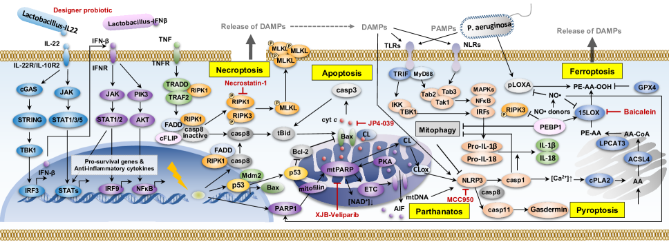
Figure 1: Distinct cell death pathways induced by irradiation exposure.

We also developed statistical model checking (SMC) techniques to calibrate and analyze ODE systems with probabilistic initial states [11, 12, 13]. In this setting, bounded linear temporal logic is used to encode quantitative behavioral constraints and qualitative properties of biochemical networks. By equipping existing parameter search algorithms with a SMC-based evaluation method, one can arrive both novel and efficient parameter estimation and analysis methods. This framework has been generalized to deal with stochastic rule-based models [14, 15] and hybrid automata [16] and applied to studies of various biological systems such as innate immune system [17] and cell death/survival pathways [18, 19, 20, 21].

However, in many settings, it is not fruitful to view the functioning of a biological system in terms of a single entity. Rather, the system will possess multiple operational modes with a specific signaling network being active in each mode. For example, signaling responses to ionizing irradiation exposure within individual cells follow distinct cell death pathways (Fig. 1). The interconnectivity between these pathways brings up new challenges on determining the sequence and timing of medication administration against radiation injuries, since interventions may alter the cellular state and induce differential modes of dynamics [22, 23, 24].

In such situations, using a monolithic approach will result in a messy and very large model with time-invariant parameters. Consequently, the modeling and analysis approach based on the notion of multi-mode biological networks will be very useful. Multi-mode dynamics and their modeling appear frequently in physical and engineering settings [25]. Multiple variants of the formalism called hybrid automata [26] are often used to model biological processes [27, 28, 29, 30, 31, 32]. However such models are difficult to analyze and to get around this, most efforts end up imposing severe restrictions on the dynamic laws associated with the modes [33, 34, 35].

In this paper, we present a novel model checking-based framework for analyzing single- or multi-mode biological systems with nonlinear dynamics (Fig. 2). Given a dynamical system, we describe the set of states of interest as a first-order logic formula and perform bounded model checking to determine reachability of these states. We adapt an interval constrains propagation (ICP) based algorithm to explore the parameter spaces and identify the sets of parameters using which the model satisfies desired behavior constraints. Note that determining the truth value of first-order sentences over the reals with nonlinear real functions is a well-known undefinable problem. We use $\delta$-decision procedures [36] to ask for answers that may have one-sided $\delta$-bounded errors. If the model satisfies the desired behavior (e.g. the model matches training and testing data), we can carry out analysis tasks such as stability analysis or identify novel therapeutic strategies using $\delta$-decision procedures. Otherwise, we will conduct SMC-based analysis [12] to generate new hypotheses and refine the model structure iteratively. We demonstrate the applicability of our framework by “proof-of-concept” studies on prostate cancer and cardiac disorders [37, 38, 39].

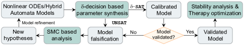
Figure 2: A model checking-enabled modeling framework.

Turning to related work, a survey of modeling and analysis of biological systems using hybrid models can be found in [40]. Formal verification of hybrid systems is a well-established domain [41]. Analyzing the properties of biochemical networks using model checking techniques is being actively pursued by a number of groups [42, 43, 44, 45]. Of particular interest in our context are parameter synthesis methods which identify parameter values for which some qualitative behavior [46, 47, 48].

The rest of the paper is organized as follows. We briefly introduce model checking in the next section. We describe the $\delta$-decision procedures in Section III. We then present the applications of $\delta$-decision-based analysis methods in Section IV. In the final section, we summarize and discuss future work.

II Model Checking

Amir Pnueli introduced temporal logics into the world of program verification [49]. The algorithmic verification procedure called model checking was formulated by Clarke and Emerson and independently by Joseph Sifakis [50]. Briefly, the model checking procedure operates as follows. Given a model $\mathcal{M}$ with initial state $s$, a model checker decides if a property written as a temporal logic formula $\phi$ is satisfied, denoted as $\mathcal{M},s\models\phi$. This can be done by: (i) constructing a finite (state) transition system corresponding to $\mathcal{M}$ in which each state represents a possible configuration of the system and each transition represents an evolution of the system from one configuration to another, and (ii) verify whether $\phi$ is satisfied by exhaustively exploring the set of system executions. The key feature of the model checking procedure is that it is fully automated. Further, if it is not the case that $\mathcal{M},s\models\phi$ then the procedure will usually return as a “counter-example” an execution due to which the property is not being met by the system. This can serve as a powerful debugging tool for systems that are large and complex. An excellent starting point for exploring this whole field is [51].

III $\delta$-Decision Procedures

III-A $\mathcal{L}_{\mathbb{R}_{\mathcal{F}}}$-Formulas and $\delta$-Decisions Over The Reals

In [36], we developed a theory of decision problems over the reals with computable functions. Most common continuous real functions are computable, including solutions of Lipschitz-continuous ODEs. In fact, the notion of computability of real functions directly corresponds to whether they can be numerically simulated. We write $\mathcal{F}$ to denote an arbitrary collection of symbols representing computable functions over $\mathbb{R}^{n}$ for various $n$. We consider the first-order formulas with a signature $\mathcal{L}_{\mathbb{R}_{\mathcal{F}}}=\langle 0,1,\mathcal{F},>\rangle$. Note that constants are seen as 0-ary functions in $\mathcal{F}$. $\mathcal{L}_{\mathbb{R}_{\mathcal{F}}}$-formulas are evaluated in the standard way over the corresponding structure $\mathbb{R}_{\mathcal{F}}=\langle\mathbb{R},\mathcal{F},>\rangle$. We use atomic formulas of the form $t(x_{1},...,x_{n})>0$ or $t(x_{1},...,x_{n})\geq 0$, where $t(x_{1},...,x_{n})$ are built up from functions in $\mathcal{F}$. To avoid extra preprocessing of formulas, we give an explicit definition of $\mathcal{L}_{\mathbb{R}_{\mathcal{F}}}$-formulas as follows.

Definition 1 ($\mathcal{L}_{\mathbb{R}_{\mathcal{F}}}$-Formulas)

Let $\mathcal{F}$ be a collection of Type 2 functions, which contains at least $0$, unary negation -, addition $+$, and absolute value $|\cdot|$. We define:

$$t :=x\;|\;f(t(\vec{x})),\mbox{ where }f\in\mathcal{F}\mbox{, possibly constant};$$

$$\varphi :=t(\vec{x})>0\;|\;t(\vec{x})\geq 0\;|\;\varphi\wedge\varphi\;|\;\varphi\vee\varphi\;|\;\exists x_{i}\varphi\;|\;\forall x_{i}\varphi.$$

In this setting $\neg\varphi$ is regarded as an inductively defined operation which replaces atomic formulas $t>0$ with $-t\geq 0$, atomic formulas $t\geq 0$ with $-t>0$, swaps $\wedge$ and $\vee$, and swaps $\forall$ and $\exists$. Implication $\varphi_{1}\rightarrow\varphi_{2}$ is defined as $\neg\varphi_{1}\vee\varphi_{2}$.

Definition 2 (Bounded Quantifiers)

We define

$$\exists^{[u,v]}x.\varphi =_{df}\exists x.(u\leq x\land x\leq v\wedge\varphi),$$

$$\forall^{[u,v]}x.\varphi =_{df}\forall x.((u\leq x\land x\leq v)\rightarrow\varphi),$$

where $u$ and $v$ denote $\mathcal{L}_{\mathbb{R}_{\mathcal{F}}}$ terms whose variables only contain free variables in $\varphi$, excluding $x$. It is easy to check that $\exists^{[u,v]}x.\varphi\leftrightarrow\neg\forall^{[u,v]}x.\neg\varphi$.

We say a sentence is bounded if it only involves bounded quantifiers.

Definition 3 (Bounded $\mathcal{L}_{\mathbb{R}_{\mathcal{F}}}$-Sentences)

A bounded $\mathcal{L}_{\mathbb{R}_{\mathcal{F}}}$-sentence is

$$Q_{1}^{[u_{1},v_{1}]}x_{1}\cdots Q_{n}^{[u_{n},v_{n}]}x_{n}\;\psi(x_{1},...,x_{n}).$$

$Q_{i}^{[u_{i},v_{i}]}$s are bounded quantifiers, and $\psi(x_{1},...,x_{n})$ is a quantifier-free $\mathcal{L}_{\mathbb{R}_{\mathcal{F}}}$-formula.

We write $\psi(x_{1},...,x_{n})$ as $\psi[t_{1}(\vec{x})>0,...,t_{k}(\vec{x})>0;t_{k+1}(\vec{x})\geq 0,...,t_{m}(\vec{x})\geq 0]$ to emphasize that $\psi(\vec{x})$ is a Boolean combination of the atomic formulas shown.

Definition 4 ($\delta$-Variants)

Let $\delta\in\mathbb{Q}^{+}\cup\{0\}$, and $\varphi$ an $\mathcal{L}_{\mathbb{R}_{\mathcal{F}}}$-formula of the form

$$\varphi:\ Q_{1}^{I_{1}}x_{1}\cdots Q_{n}^{I_{n}}x_{n}\;\psi[t_{i}(\vec{x},\vec{y})>0;t_{j}(\vec{x},\vec{y})\geq 0],$$

where $i\in\{1,...k\}$ and $j\in\{k+1,...,m\}$. The $\delta$-weakening $\varphi^{\delta}$ of $\varphi$ is defined as the result of replacing each atom $t_{i}>0$ by $t_{i}>-\delta$ and $t_{j}\geq 0$ by $t_{j}\geq-\delta$. That is,

$$\varphi^{\delta}:\ Q_{1}^{I_{1}}x_{1}\cdots Q_{n}^{I_{n}}x_{n}\;\psi[t_{i}(\vec{x},\vec{y})>-\delta;t_{j}(\vec{x},\vec{y})\geq-\delta].$$

We then have the following main decidability result.

Theorem 1 ($\delta$-Decidability)

Let $\delta\in\mathbb{Q}^{+}$ be arbitrary. There is an algorithm which, given any bounded $\varphi$, correctly returns one of the following two answers:

• $\phi$ is false ($\mathsf{unsat}$);

• $\phi^{\delta}$ is true ($\delta$-$\mathsf{sat}$).

Note when the two cases overlap, either answer is correct.

We call this new decision problem the $\delta$-decision problem for $\mathcal{L}_{\mathbb{R}_{\mathcal{F}}}$-sentences.

Definition 5 ($\delta$-Complete Decision Procedures)

If an algorithm solves the $\delta$-decision problem correctly for a set $S$ of $\mathcal{L}_{\mathbb{R}_{\mathcal{F}}}$-sentences, we say it is $\delta$-complete for $S$.

From $\delta$-decidability, $\delta$-complete decision procedures always exist for bounded $\mathcal{L}_{\mathbb{R}_{\mathcal{F}}}$-formulas. In practice, we have shown that the combination of the DPLL(T) framework and ICP indeed gives us a $\delta$-complete decision procedure [52].

III-B Parameterized $\mathcal{L}_{\mathbb{R}_{\mathcal{F}}}$-Representations of Hybrid Automata

We now describe hybrid automata using $\mathcal{L}_{\mathbb{R}_{\mathcal{F}}}$-formulas, and define parameterization and perturbations on them.

A hybrid system is a tuple $H=\langle X$, $Q$, $\mathsf{flow}$, $\mathsf{guard}$, $\mathsf{reset}$, $\mathsf{inv}$, $\mathsf{init}\rangle$ where $X\subseteq\mathbb{R}^{n}$ specifies the range of the continuous variables $\vec{x}$ of the system. $Q=\{q_{0},...,q_{m}\}$ is a finite set of discrete control modes. $\mathsf{flow}\subseteq Q\times X\times\mathbb{R}\times X$ specifies the continuous dynamics for each mode. The $\mathsf{flow}$ predicate is usually defined either as explicit mappings from $\vec{a}_{0}$ and $t$ to $\vec{a}_{t}$, or as solutions of systems of differential equations/inclusions that specify the derivative of $\vec{x}$ over time. $\mathsf{jump}\subseteq Q\times X\times Q\times X$ specifies the jump conditions between modes. $\mathsf{inv}\subseteq Q\times X$ defines the invariant conditions for the system to stay in a control mode. $\mathsf{init}\subseteq Q\times X$ defines the set of initial configurations of the system. Without loss of generality we always assume that $q_{0}$ is the only intial mode, and $\mathsf{init}_{q_{0}}\subseteq X$ denotes the initial values for the continuous variables.

Definition 6 ($\mathcal{L}_{\mathbb{R}_{\mathcal{F}}}$-Representations)

Let $H=\langle X$, $Q$, $\mathsf{flow}$, $\mathsf{jump}$, $\mathsf{inv}$, $\mathsf{init}\rangle$ be an $n$-dimensional hybrid automaton. Let $\mathcal{F}$ be a set of real functions, and $\mathcal{L}_{\mathbb{R}_{\mathcal{F}}}$ the corresponding first-order language. We say that $H$ has an $\mathcal{L}_{\mathbb{R}_{\mathcal{F}}}$-representation, if for every $q,q^{\prime}\in Q$, there exists quantifier-free $\mathcal{L}_{\mathbb{R}_{\mathcal{F}}}$-formulas

$$\phi^{q}_{\mathsf{flow}}(\vec{x},\vec{x}_{0},t),\phi^{q\rightarrow q^{\prime}}_{\mathsf{jump}}(\vec{x},\vec{x}^{\prime}),\phi^{q}_{\mathsf{inv}}(\vec{x}),\phi^{q}_{\mathsf{init}}(\vec{x})$$

such that for all $\vec{a},\vec{a}^{\prime}\in\mathbb{R}^{n}$, $t\in\mathbb{R}$:

• $\mathbb{R}\models\phi^{q}_{\mathsf{flow}}(\vec{a},\vec{a}^{\prime},t)$ iff $(q,\vec{a},\vec{a}^{\prime},t)\in\mathsf{flow}$.

• $\mathbb{R}\models\phi^{q\rightarrow q^{\prime}}_{\mathsf{jump}}(\vec{a},\vec{a}^{\prime})$ iff $(q,q^{\prime},\vec{a},\vec{a}^{\prime})\in\mathsf{jump}$.

• $\mathbb{R}\models\phi^{q}_{\mathsf{inv}}(\vec{a})$ iff $(q,\vec{a})\in\mathsf{inv}.$

• $\mathbb{R}\models\phi^{q}_{\mathsf{init}}(\vec{a})$ iff $q=q_{0}$ and $\vec{a}\in\mathsf{init}_{q_{0}}$.

We can write $H=\langle X,Q,\phi_{\mathsf{flow}},\phi_{\mathsf{jump}},\phi_{\mathsf{inv}},\phi_{\mathsf{init}}\rangle$ to emphasize that $H$ is $\mathcal{L}_{\mathbb{R}_{\mathcal{F}}}$-represented. But from now on we simply write $\mathsf{flow},\mathsf{jump},\mathsf{inv},\mathsf{init}$ to denote these logic formulas, so that we can use $H=\langle X,Q,\mathsf{flow},\mathsf{jump},\mathsf{inv},\mathsf{init}\rangle$ directly to denote the $\mathcal{L}_{\mathbb{R}_{\mathcal{F}}}$-representation of $H$.

Definition 7 (Computable Representation)

We say a hybrid automaton $H$ has a computable representation, if $H$ has an $\mathcal{L}_{\mathbb{R}_{\mathcal{F}}}$-representation, where $\mathcal{F}$ is an arbitrary set of computable functions.

Combining continuous and discrete behaviors, the trajectories of hybrid systems are piecewise continuous. This motivates a two-dimensional structure of time, with which we can keep track of both the discrete changes and the duration of each continuous flow.

Definition 8 (Hybrid Time Domain)

A hybrid time domain $T$ is a subset of $\mathbb{N}\times\mathbb{R}$ of the form $T_{m}=\{(i,t):i<m\mbox{ and }t\in[t_{i},t_{i}^{\prime}]\mbox{ or }[t_{i},+\infty)\},$ where $m\in\mathbb{N}\cup\{+\infty\}$, $\{t_{i}\}_{i=0}^{m}$ is an increasing sequence in $\mathbb{R}^{+}$, $t_{0}=0$, and $t_{i}^{\prime}=t_{i+1}$.

We write the set of all hybrid time domains as $\mathbb{H}$.

Definition 9 (Hybrid Trajectories)

Suppose $X\subseteq\mathbb{R}^{n}$ and $T_{m}$ is a hybrid time domain. A hybrid trajectory is any continuous function $\xi:T_{m}\rightarrow X.$

We write $\Xi_{X}$ to denote the set of all possible hybrid trajectories from $\mathbb{H}$ to $X$. We can now define trajectories of a given hybrid automaton. The intuition behind the following definition is straightforward. The labeling function $\sigma_{\xi}^{H}(i)$ is used to map a step $i$ to the corresponding discrete mode in $H$. In each mode, the system flows continuously following the dynamics defined by $\mathsf{flow}(q,\vec{x}_{0},t)$. Note that $(t-t_{k})$ is the actual duration in the $k$-th mode. When a switch between two modes is performed, it is required that $\xi(k+1,t_{k+1})$ is updated from the exit value $\xi(k,t_{k}^{\prime})$ in the previous mode, following the jump conditions.

Definition 10 (Trajectories of a Hybrid Automaton)

Let $H$ be a hybrid automaton, and $\xi:T_{m}\rightarrow X$ a hybrid trajectory. We say that $\xi:T_{m}\rightarrow X$ is a trajectory of $H$ of discrete depth $m$, if there exists a labeling function $\sigma^{H}_{\xi}:\mathbb{N}\rightarrow Q$ such that:

• $\sigma^{H}_{\xi}(0)=q_{0}$ and $\mathbb{R}_{\mathcal{F}}\models\mathsf{init}_{q_{0}}(\xi(0,0))$.

• For any $(i,t)\in T_{m}$, $\mathbb{R}_{\mathcal{F}}\models\mathsf{inv}_{\sigma^{H}_{\xi}(i)}(\xi(i,t))$.

• When $i=0$, $\mathbb{R}_{\mathcal{F}}\models\mathsf{flow}_{q_{0}}(\xi(0,0),\xi(0,t),t)$.

• When $i=k+1$, where $0<k+1<m$,

  $$\mathbb{R}_{\mathcal{F}} \models \mathsf{flow}_{\sigma^{H}_{\xi}(k+1)}(\xi(k+1,t_{k+1}),\xi(k+1,t),$$

  $$(t-t_{k+1}))\mbox{ and }$$

  $$\mathbb{R}_{\mathcal{F}} \models \mathsf{jump}_{(\sigma^{H}(k)\rightarrow\sigma^{H}(k+1))}(\xi(k,t_{k}^{\prime}),\xi(k+1,t_{k+1})).$$

We write $\llbracket H\rrbracket$ to denote all possible trajectories of $H$.

Definition 11 (Reachability Properties)

Let $H$ be a hybrid automaton and $U\subseteq X\times Q$ be a subset of its state space. Let $U\subseteq X\times Q$ be a subset of the state space of $H$. $H$ reaches $U$ if there exists $\xi\in\llbracket H\rrbracket$ such that there exists $t\in\mathbb{R}$ and $n\in\mathbb{N}$ satisfying

$$(\xi(t,n),\sigma_{\xi}^{H}(n))\in U.$$

Let $H$ be a hybrid system. Parameter synthesis for reachability properties asks for a set of parameters such that some mode can be reached.

Definition 12 (Parameterized Hybrid Automaton)

We say a hybrid automaton $H$ is parameterized by $\vec{p}$, if We say $H$ is parameterized by $\vec{p}=(p_{1},...,p_{m})$, if

$$H(\vec{p})=\langle X,Q,\mathsf{flow}(\vec{p}),\mathsf{jump}(\vec{p}),\mathsf{inv}(\vec{p}),\mathsf{init}(\vec{p})\rangle,$$

where $\vec{p}$ are among the free variables in the $\mathcal{L}_{\mathbb{R}_{\mathcal{F}}}$-representation of $H$.

Definition 13 (Parameter Synthesis for Reachability Properties)

Let $H(\vec{p})$ be a hybrid automaton parameterized by variables $\vec{p}=(p_{1},...,p_{m})$, and $U\subseteq X\times Q$ a subset of its state space. Thus, the parameter synthesis problem for reachability asks for an assignment for $\vec{a}\in\mathbb{R}^{m}$ such that $H(\vec{a})$ reaches $U$.

III-C Synthesizing Parameters with $\delta$-Decisions

We now show how to encode parameter synthesis problems for $\mathcal{L}_{\mathbb{R}_{\mathcal{F}}}$-represented hybrid systems using $\mathcal{L}_{\mathbb{R}_{\mathcal{F}}}$-formulas. Throughout the following two definitions, let $H=\langle X$, $Q$, $\mathsf{flow}$, $\mathsf{jump}$, $\mathsf{init}\rangle$ be an $n$-dimensional $\mathcal{L}_{\mathbb{R}_{\mathcal{F}}}$-represented hybrid system with $|Q|=m$, and $\mathsf{unsafe}$ an $\mathcal{L}_{\mathbb{R}_{\mathcal{F}}}$-formula that encodes a subset $U\subseteq X\times Q$. Let $k\in\mathbb{N}$ and $M\in\mathbb{R}$ be the bounds on steps and time respectively. Recall that $q_{0}\in Q$ always denotes the starting mode.

$\mathsf{Reach}_{H,q^{\prime}}^{k}(\vec{x}_{k}^{t})$ defines the states that $H$ can reach, if after $k$ steps of discrete changes it is in mode $q^{\prime}$. From there, if $H$ makes a $\mathsf{jump}$ from mode $q^{\prime}$ to $q$, then the states have to make a discrete change following $\mathsf{jump}_{q^{\prime}\rightarrow q}(\vec{x}_{k}^{t},\vec{x}_{k+1})$. As last, in mode $q^{\prime}$, any state $\vec{x}_{k+1}^{t}$ that $H$ can reach should satisfy the $\mathsf{flow}$ conditions $\mathsf{flow}_{q}(\vec{x}_{k+1}^{t},\vec{x}_{k+1},t)$ in mode $q$. Note that after each discrete jump, a new time variable $t_{k}$ is introduced and independent from the previous ones.

The $(k,M)$-reachability encoding of $H$ and $U$, $\mathsf{Reach}^{k,M}(H,U)$, is defined as:

$$\exists\vec{a}\exists^{X}\vec{x}_{0}\exists^{X}\vec{x}_{0}^{t}\cdots\exists^{X}\vec{x}_{k}\exists^{X}\vec{x}_{k}^{t}\exists^{[0,M]}t_{0}\cdots\exists^{[0,M]}t_{k}$$

$$\Big{(}\ \mathsf{init}_{q_{0}}(\vec{x}_{0})\wedge\mathsf{flow}_{q_{0}}(\vec{a},\vec{x}_{0},\vec{x}_{0}^{t},t_{0})$$

$$\wedge\forall^{[0,t_{0}]}t\forall^{X}\vec{x}\;(\mathsf{flow}_{q_{0}}(\vec{a},\vec{x}_{0},\vec{x},t)\rightarrow\mathsf{inv}_{q_{0}}(\vec{a},\vec{x}))$$

$$\wedge\bigvee_{i=0}^{k-1}\Big{(}\bigvee_{q,q^{\prime}\in Q}\Big{(}\mathsf{jump}_{q\rightarrow q^{\prime}}(\vec{a},\vec{x}_{i}^{t},\vec{x}_{i+1})\wedge\mathsf{flow}_{q^{\prime}}(\vec{a},\vec{x}_{i+1},\vec{x}_{i+1}^{t},t_{i+1})$$

$$\wedge\forall^{[0,t_{0}]}t\forall^{X}\vec{x}\;(\mathsf{flow}_{q^{\prime}}(\vec{a},\vec{x}_{i+1},\vec{x},t)\rightarrow\mathsf{inv}_{q_{0}}(\vec{a},\vec{x})))\Big{)}\Big{)}$$

$$\wedge\ \mathsf{unsafe}(\vec{a},\vec{x}_{k}^{t})\Big{)}.$$

$H$ reaches $U$ in $k$ steps of discrete jumps with time duration less than $M$ for each state iff $\mathsf{Reach}^{k,M}(H,U)$ is true.

IV Applications

IV-A Model Calibration and Falsification

The $\delta$-decision problems can be solved using our dReal tool [52]. Parameter estimation of single-mode ODE models can be encoded as SMT formulas by BioPSy [53] and solved by dReal, while for multi-mode models we ask a $k$-step reachability question: Is there a set of parameter values using which the model reaches the goal region in $k$ steps? The dReach tool [54] can automatically build such reachability formulas from a multi-mode model and a goal description, which are then verified by dReal. If $\mathsf{unsat}$ is returned, the model is unfeasible, which means that the model is unable to satisfy a desired behavior no matter which parameter values are used. This can be used to reject model hypotheses. For example, we have showed that the Fenton-Karma model [55] of cardiac cells is unable to reproduce the “spike-and-dome” morphology of action potential which has been observed in epicardial cells [37]. On the other hand, if the model is $\delta$-$\mathsf{sat}$, a witness (i.e. a set of parameter values) is returned. For example, using the Bueno-Cherry-Fenton model [56], we have identified critical parameter ranges that can cause cardiac disorders such as tachycardia and fibrillation [37].

IV-B Identification of Therapeutic Strategies

The $\delta$-decision procedures can be used to design optimal therapeutic strategies. For example, Fig. 3 illustrates a multi-mode model of the TBI-induced signaling network shown in Fig. 1. The starting point Mode 0 corresponds to live cells under no treatment for 24 h after TBI. Mode 1 is the “point of no return” which leads to cell death. Modes A-E represent live cells subjected to particular treatments (e.g. Balcalein-induced ferroptosis inhibition). The jump conditions are defined by the molecular signature. For example, starting with Mode 0, if the oxidized CL level exceeds a threshold $\theta_{1}$, the system jumps to Mode A, which means that we deliver the apoptosis inhibitor JP4-039. The system then evolves according to the ODEs in Mode A, until another jump condition–e.g. the level of activated RIP3 above threshold $\theta_{2}$–is reached, which implies the onset of necroptosis, or Mode B. We then deliver necroptosis inhibitor necrostatin-1. Suppose the system next jumps back to Mode 0 and stays. The mode path $0\rightarrow A\rightarrow B\rightarrow 0$ suggests a successful treatment scheme defined by a set of jump conditions. Note that we also aim to minimize the number of drugs used (i.e. path length) to avoid potential side effects. Thus, the problem of determining which drug to deliver at what time, evolves into a parameter synthesis problem for hybrid automata and can be tackled by $\delta$-decision procedures. In a “proof-of-concept” study [38], we have used this approach to identity personalized therapeutic strategies for prostate cancer patients.

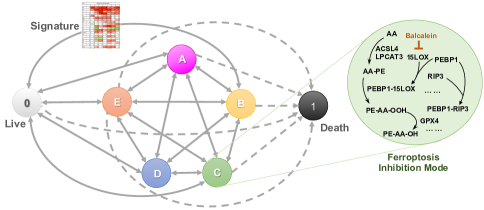
Figure 3: Multi-mode modeling. Mode 0: live cell, no treatment; Mode A: apoptosis inhibition; Mode B: necroptosis inhibition; Mode C: Ferroptosis inhibition; Mode D: Pyroptosis inhibition; Mode E: Parthanatos inhibition Mode 1: dead cell.

IV-C Stability Analysis

The robustness of biological systems often refers to the consistency of system behavior in response to small perturbations. For example, cardiac cells filter out insignificant stimulations to ensure proper functioning in noisy environments. Using the $\delta$-decision procedures, we can verify this by checking if the action potential can be successfully triggered by a small range of stimulation. An $\mathsf{unsat}$ answer returned by dReach will guarantee that the model is robust to the corresponding stimulation amplitude [37].

In addition to “time-bounded” robustness, the $\delta$-decision procedures can also be used to analyze the infinite-time stability of nonlinear dynamical systems [57, 58]. Such stability–often referred as structural stability–exists in the systems that have unique globally asymptotically stable steady states. A standard way of verifying this property is to find a Lyapunov function [59] that provides theoretical guarantees on qualitative behavior of the system. Lyapunov-enable analysis has been applied to mass-action law based kinetic models of signaling networks such as T-cell kinetic proofreading and ERK signaling [60]. Our $\delta$-decision procedures enable the Lyapunov stable analysis for systems with non-polynomial nonlinearity in two ways: (i) Given a template function, we can synthesize a Lyapunov function by solving $\exists\forall$-formulas that encode the corresponding non-convex, multi-objective and disjunctive optimization problem [57]; (ii) We can provide a sound and relative-complete proof system for induction rules that robustify the standard notions of Lyapunov functions [58].

V Conclusion and Future Works

We have presented a model checking-enabled framework for analyzing systems biology models with the help of $\delta$-decision procedures. We used the $\mathcal{L}_{\mathbb{R}_{\mathcal{F}}}$-formulas to describe parameterized hybrid automata and encode parameter synthesis problems. We employed the $\delta$-decision procedures to perform bounded model checking and obtain parameters using which the model can satisfy desired properties. We have showed that the $\delta$-decision procedures can be used to estimate unknown model parameters, reject model hypothesis, analyze the model’s Lyapunov stability, as well as design combination therapies. These tasks can be assembled as a unified workflow for understanding the mechanism of diseases and identifying therapeutic options. Our preliminary studies on prostate cancer, cardiac disorders, and radiation diseases have shown promising results.

An interesting direction is extending our method for probabilistic settings to address the inherent variability in biological systems. To cope with the model complexity, an idea is to approximate the hybrid system as a multi-mode network of DBNs by extending the approximation technique we have developed for a single system of ODEs [5]. We plan to explore this in our future work. In this respect, the Chow-Liu tree representation-based approximation scheme used in [61] promises to offer helpful pointers.

References

- [1] P. K. Sorger and B. Schoeberl, “An expanding role for cell biologists in drug discovery and pharmacology,” Mol. Biol. Cell, vol. 23, no. 21, pp. 4162–4164, 2012.
- [2] B. Liu and P. S. Thiagarajan, “Modeling and Analysis of Biopathways Dynamics,” J. Bioinf. Comput. Biol., vol. 10, no. 4, p. 1231001, 2012.
- [3] B. Liu, P. Thiagarajan, and D. Hsu, “Probabilistic approximations of signaling pathway dynamics,” in CMSB’09, 2009, pp. 251–265.
- [4] B. Liu, D. Hsu, and P. Thiagarajan, “Probabilistic approximations of ODEs based bio-pathway dynamics,” Theor. Comput. Sci., vol. 412, no. 21, pp. 2188–2206, 2011.
- [5] B. Liu et al., “Approximate probabilistic analysis of biopathway dynamics,” Bioinformatics, vol. 28, no. 11, pp. 1508–1516, 2012.
- [6] A. Hagiescu et al., “GPU code generation for ODE-based applications with phased shared-data access patterns,” ACM Trans. Archit. Code Optim, vol. 10, no. 4, pp. 1–19, 2013.
- [7] S. K. Palaniappan, S. Akshay, B. Liu, B. Genest, and P. Thiagarajan, “A hybrid factored frontier algorithm for dynamic bayesian networks with a biopathways application,” IEEE/ACM Trans. Comput. Biol. Bioinform., vol. 9, no. 5, pp. 1352–1365, 2012.
- [8] S. K. Palaniappan, M. Pichené, G. Batt, E. Fabre, and B. Genest, “A look-ahead simulation algorithm for dbn models of biochemical pathways,” in HSB’16, 2016, pp. 3–19.
- [9] B. Liu et al., “A computational and experimental study of the regulatory mechanisms of the complement system,” PLoS Comput. Biol., vol. 7, no. 1, 2011.
- [10] S. K. Palaniappan, F. Bertaux, M. Pichené, E. Fabre, G. Batt, and B. Genest, “Abstracting the dynamics of biological pathways using information theory: a case study of apoptosis pathway,” Bioinformatics, vol. 33, no. 13, pp. 1980–1986, 2017.
- [11] S. K. Palaniappan, B. M. Gyori, B. Liu, D. Hsu, and P. S. Thiagarajan, “Statistical model checking based calibration and analysis of bio-pathway models,” in CMSB’13, vol. 8130 LNCS, 2013, pp. 120–134.
- [12] B. Liu, B. M. Gyori, and P. Thiagarajan, “Statistical model checking-based analysis of biological networks,” in Automated Reasoning for Systems Biology and Medicine, 2019, pp. 63–92.
- [13] R. Ramanathan, Y. Zhang, J. Zhou, B. M. Gyori, W.-F. Wong, and P. Thiagarajan, “Parallelized parameter estimation of biological pathway models,” in HSB’15, 2015, pp. 37–57.
- [14] B. Liu and J. R. Faeder, “Parameter estimation of rule-based models using statistical model checking,” in BIBM’16, 2016, pp. 1453–1459.
- [15] Q. Wang, N. Miskov-Zivanov, B. Liu, J. R. Faeder, M. Lotze, and E. M. Clarke, “Formal modeling and analysis of pancreatic cancer microenvironment,” in CMSB’16, 2016, pp. 289–305.
- [16] B. M. Gyori, B. Liu, S. Paul, R. Ramanathan, and P. Thiagarajan, “Approximate probabilistic verification of hybrid systems,” in HSB’15, 2015, pp. 96–116.
- [17] B. Liu, Q. Liu, S. Palaniappan, I. Bahar, P. S. Thiagarajan, and J. L. Ding, “Innate Immune Memory and Homeostasis May Be Conferred Through TLR3-TLR7 Pathway Crosstalk,” Sci. Signal., vol. 9, no. 436, p. ra70, 2016.
- [18] B. Liu, D. Bhatt, Z. N. Oltvai, J. S. Greenberger, and I. Bahar, “Significance of p53 dynamics in regulating apoptosis in response to ionizing radiation, and polypharmacological strategies.” Sci. Rep., vol. 4, p. 6245, 2014.
- [19] B. Liu et al., “Quantitative assessment of cell fate decision between autophagy and apoptosis,” Sci. Rep., vol. 7, no. 1, pp. 1–14, 2017.
- [20] V. E. Kagan et al., “Oxidized arachidonic and adrenic pes navigate cells to ferroptosis,” Nat. Chem. Biol., vol. 13, no. 1, p. 81, 2017.
- [21] A. A. Kapralov et al., “Redox lipid reprogramming commands susceptibility of macrophages and microglia to ferroptotic death,” Nat. Chem. Biol., vol. 16, no. 3, pp. 278–290, 2020.
- [22] J. Steinman et al., “Improved total-body irradiation survival by delivery of two radiation mitigators that target distinct cell death pathways,” Radiat. Res, vol. 189, no. 1, pp. 68–83, 2018.
- [23] S. Thermozier et al., “Radioresistance of serpinb3a-/- mice and derived hematopoietic and marrow stromal cell lines,” Radiat. Res., vol. 192, no. 3, pp. 267–281, 2019.
- [24] ——, “Anti-ferroptosis drug enhances total-body irradiation mitigation by drugs that block apoptosis and necroptosis,” Radiat. Res., p. [Epub ahead of print], 2020.
- [25] R. Goebel, R. G. Sanfelice, and A. R. Teel, “Hybrid dynamical systems,” IEEE Contr. Syst. Mag., vol. 29, no. 2, pp. 28–93, 2009.
- [26] T. A. Henzinger, “The theory of hybrid automata,” in LICS’96, Washington, DC, USA, 1996, pp. 278–292.
- [27] R. Ghosh and C. Tomlin, “Symbolic reachable set computation of piecewise affine hybrid automata and its application to biological modelling: Delta-notch protein signalling,” IET Syst. Biol., vol. 1, no. 1, pp. 170–183, 2004.
- [28] P. Ye, E. Entcheva, S. Smolka, and R. Grosu, “Modelling excitable cells using cycle-linear hybrid automata,” IET Syst. Biol., vol. 2, no. 1, pp. 24–32, 2008.
- [29] K. Aihara and H. Suzuki, “Theory of hybrid dynamical systems and its applications to biological and medical systems,” Philos. Trans. R. Soc. London, Ser. A, vol. 368, no. 1930, pp. 4893–4914, 2010.
- [30] M. Antoniotti, B. Mishra, C. Piazza, A. Policriti, and M. Simeoni, “Modeling cellular behavior with hybrid automata: Bisimulation and collapsing,” in CMSB’03, 2003, pp. 57–74.
- [31] P. Lincoln and A. Tiwari, “Symbolic systems biology: Hybrid modeling and analysis of biological networks,” in HSCC’04, 2004, pp. 660–672.
- [32] V. Baldazzi, P. T. Monteiro, M. Page, D. Ropers, J. Geiselmann, and H. De Jong, “Qualitative analysis of genetic regulatory networks in bacteria,” in Understanding the Dynamics of Biological Systems, 2011, pp. 111–130.
- [33] E. Clarke, A. Fehnker, Z. Han, B. Krogh, O. Stursberg, and M. Theobald, “Verification of hybrid systems based on counterexample-guided abstraction refinement,” in TACAS’03, 2003, pp. 192–207.
- [34] T. A. Henzinger and P. W. Kopke, “Discrete-time control for rectangular hybrid automata,” Theor. Comput. Sci., vol. 221, no. 1, pp. 369–392, 1999.
- [35] M. Agrawal, F. Stephan, P. Thiagarajan, and S. Yang, “Behavioural approximations for restricted linear differential hybrid automata,” in HSCC’06, 2006, pp. 4–18.
- [36] S. Gao, J. Avigad, and E. M. Clarke, “Delta-complete decision procedures for satisfiability over the reals,” in IJCAR’12, 2012, pp. 286–300.
- [37] B. Liu, S. Kong, S. Gao, P. Zuliani, and E. M. Clarke, “Parameter synthesis for cardiac cell hybrid models using -decisions,” in CMSB’14, vol. 8859 LNCS, 2014, pp. 99–113.
- [38] ——, “Towards personalized prostate cancer therapy using delta-reachability analysis,” in HSCC’15, 2015, pp. 227–232.
- [39] B. Liu, S. Kong, S. Gao, and E. Clarke, “Parameter identification using delta-decisions for biological hybrid systems,” Carnegie Mellon Univ., Tech. Rep. CMU-CS-13-136, 2013.
- [40] L. Bortolussi and A. Policriti, “Hybrid systems and biology,” in Formal Methods for Computational Systems Biology, 2008, pp. 424–448.
- [41] R. Alur, “Formal verification of hybrid systems,” in EMSOFT’ 11, Taipei, Taiwan, 2011, pp. 1–6.
- [42] E. M. Clarke, J. R. Faeder, C. J. Langmead, L. A. Harris, S. K. Jha, and A. Legay, “Statistical model checking in BioLab: Applications to the automated analysis of T-Cell receptor signaling pathway,” in CMSB’08, 2008, pp. 231–250.
- [43] N. Chabrier-Rivier, M. Chiaverini, V. Danos, F. Fages, and V. Schächter, “Modeling and querying biomolecular interaction networks,” Theor. Comput. Sci., vol. 325, no. 1, pp. 25–44, sep 2004.
- [44] M. Kwiatkowska, G. Norman, and D. Parker, “Using probabilistic model checking in systems biology,” SIGMETRICS Perform. Eval. Rev., vol. 35, no. 4, pp. 14–21, 2008.
- [45] C. Li, M. Nagasaki, C. H. Koh, and S. Miyano, “Online model checking approach based parameter estimation to a neuronal fate decision simulation model in Caenorhabditis elegans with hybrid functional Petri net with extension,” Mol. Biosyst., vol. 11(Suppl 7), pp. 1–13, 2010.
- [46] G. Batt, C. belta, and R. Weiss, “Temporal logic analysis of gene networks under parameter uncertainty,” IEEE T. Automat. Contr., vol. 53, pp. 215–229, 2008.
- [47] A. Donze, G. Clermont, and C. J. Langmead, “Parameter synthesis in nonlinear dynamical systems: Application to systems biology,” J Comput. Biol., vol. 17, no. 3, pp. 325–336, 2010.
- [48] A. Khalid and S. K. Jha, “Calibration of rule-based stochastic biochemical models using statistical model checking,” in BIBM’18. IEEE, 2018, pp. 179–184.
- [49] A. Pnueli, “The temporal logic of programs,” in SFCS’77, 1977, pp. 46–57.
- [50] E. M. Clarke, “The birth of model checking,” in 25 Years of Model Checking, 2008, pp. 1–26.
- [51] E. M. Clarke Jr, O. Grumberg, D. Kroening, D. Peled, and H. Veith, Model Checking. MIT Press, 2018.
- [52] S. Gao, S. Kong, and E. M. Clarke, “dReal: An SMT solver for nonlinear theories of reals,” in CADE’13, 2013, pp. 208–214.
- [53] C. Madsen, F. Shmarov, and P. Zuliani, “Biopsy: an smt-based tool for guaranteed parameter set synthesis of biological models,” in CMSB’15, 2015, pp. 182–194.
- [54] S. Kong, S. Gao, W. Chen, and E. Clarke, “dreach: -reachability analysis for hybrid systems,” in TACAS’15, 2015, pp. 200–205.
- [55] F. Fenton and A. Karma, “Vortex dynamics in 3D continuous myocardium with fiber rotation: filament instability and fibrillation,” Chaos, vol. 8, pp. 20–47, 1998.
- [56] A. Bueno-Orovio, E. M. Cherry, and F. H. Fenton, “Minimal model for human ventricular action potentials in tissue,” J. Theor. Biol., vol. 253, pp. 544–560, 2008.
- [57] S. Kong, A. Solar-Lezama, and S. Gao, “Delta-decision procedures for exists-forall problems over the reals,” in CAV’18, 2018, pp. 219–235.
- [58] S. Gao et al., “Numerically-robust inductive proof rules for continuous dynamical systems,” in CAV’19, 2019, pp. 137–154.
- [59] E. D. Sontag, Mathematical control theory: deterministic finite dimensional systems, 2nd ed. Springer, New York, 1998.
- [60] M. A. Al-Radhawi, D. Angeli, and E. D. Sontag, “A computational framework for a Lyapunov-enabled analysis of biochemical reaction networks,” PLoS Comput. Biol., vol. 16, no. 2, p. e1007681, 2020.
- [61] M. Pichené, S. K. Palanniappan, E. Fabre, and B. Genest, “Modeling variability in populations of cells using approximated multivariate distributions,” IEEE/ACM Trans. Comput. Biol. Bioinform., pp. 1–12, 2019.