Semi-Supervised Neural System for Tagging, Parsing and Lemmatization

Abstract

This paper describes the ICS PAS system which took part in CoNLL 2018 shared task on Multilingual Parsing from Raw Text to Universal Dependencies. The system consists of jointly trained tagger, lemmatizer, and dependency parser which are based on features extracted by a biLSTM network. The system uses both fully connected and dilated convolutional neural architectures. The novelty of our approach is the use of an additional loss function, which reduces the number of cycles in the predicted dependency graphs, and the use of self-training to increase the system performance. The proposed system, i.e. ICS PAS (Warszawa), ranked 3th/4th in the official evaluation obtaining the following overall results: 73.02 (LAS), 60.25 (MLAS) and 64.44 (BLEX).

1 Introduction

Most of contemporary NLP systems for machine translation, question answering, sentiment analysis, etc. operate on preprocessed texts, i.e. texts with tokenised, part-of-speech tagged, and possibly syntactically parsed sentences. Therefore, the development of high-quality pipelines of NLP tools or entire systems for language preprocessing is still an important issue. The vast majority of language preprocessing frameworks take advantage of the statistical methods, especially the supervised or semi-supervised statistical methods. Based on training data, language preprocessing tools learn to analyse sentences and to predict morphosyntactic annotations of these sentences.

The supervised methods require gold-standard training data whose creation is a time-consuming and expensive process. Nevertheless, the morphosyntactically annotated data sets are publicly available for many languages, in particular within Universal Dependencies initiative (UD, Nivre et al., 2016). The initiators of UD aim at developing a cross-linguistically consistent annotation schema and at building a large multilingual collection of sentences annotated according to this schema with the universal part-of-speech tags and the universal dependency trees.

UD treebanks are nowadays used for multilingual system development Nivre et al. (2018). The history of developing multilingual systems dates back to 2006 and 2007, when two shared tasks on multilingual dependency parsing were organised at the Conference on Computational Natural Language Learning (CoNLL, Buchholz and Marsi, 2006; Nivre et al., 2007). After 10 years, the shared task was organised again in 2017 Zeman et al. (2017), and currently there is its fourth edition Zeman et al. (2018).

In this paper we describe our solution submitted to the CoNLL 2018 Universal Dependency shared task. The system and the trained models for participating treebanks are publicly available. Our system takes a tokenised sentence as input. The sentence tokenisation is predicted by the baseline model Straka and Straková (2017).

Each word is represented both as an external word embedding and as a character-based word embedding estimated by a dilated convolutional neural network encoder (CNN, Yu and Koltun, 2016). The concatenation of these embeddings is fed to a bidirectional long short-term memory network (biLSTM, Graves and Schmidhuber, 2005; Hochreiter and Schmidhuber, 1997) which extracts the final features (see Section 2.1). The tagger takes extracted features and predicts universal part-of-speech tags, language-specific tags and morphological features using three separate fully connected neural networks with one hidden layer (see Section 2.2). The lemmatizer uses a dilated CNN to predict lemmas based on characters of corresponding words and features previously extracted by a biLSTM encoder (see Section 2.3). As a scoring function, the graph-based dependency parser uses simple dot product of the vector representations of a dependent and its governor. These representations are output by two single fully connected layers which take feature vectors extracted by a biLSTM encoder as input. A novel loss function penalizes cycles, in order to reduce their number in the predicted dependency graphs (see Section 2.4.2). Chu-Liu-Edmonds algorithm Chu and Liu (1965); Edmonds (1967) constructs the final dependency tree. The dependency labels are predicted with a fully connected neural network based on the dependent and its governor embeddings as well (see Section 2.4 for more details on the parser’s architecture). The system architecture is schematised in Figure 1.

Figure 1: The schema of the system architecture.

The whole system is end-to-end trained, separately for each treebank provided for the purposes of the shared task. The technical details of the implemented system are given in Section 3. Additionally, for 20 selected treebanks self-training is used to increase the performance of the models (see Section 3.4). The proposed technique of self-training has an impact on the quality of tagging, lemmatisation and parsing (see Section 4.3). The article ends with the presentation of the results achieved by our system (see Section 4) and some conclusions (see Section 5).

2 Architecture Overview

2.1 Feature Extraction

The system accepts an input in the form of tokenised sentences that can be annotated with additional morphosyntactic information: lemmas, part-of-speech tags, and morphological features. However, as the goal of the shared task is to predict not only dependency trees but also parts of speech, lemmas and morphological features, we decide to use words as the only input.

2.1.1 Word Level Embedding

Each input word is represented as a vector using the external pre-trained embedding. Words not present in the external embedding are replaced with the “unknown” word and represented as a random vector drawn from the normal distribution with the mean and the variance calculated based on other word embedding vectors. Both the external embedding itself and the vector representing “unknown” word are fixed during the training, but they are transformed by a single fully connected layer. This transformation serves similar purpose as a trainable embedding, but helps with generalization, since it will also transform vectors for words available in the external embedding, but not in the training set.

2.1.2 Character Level Embedding

Additionally, each word is represented as the character-based word embedding extracted with a dilated convolutional neural network (CNN). We decide to use the dilated CNN instead of commonly used biLSTM encoder to speed up the training of the system.

First, each word is transformed to a sequence of the trainable character embeddings. Moreover, the special symbols “beginning-of-word” and “end-of-word” are added to the sequence to represent the beginning and the end of the word. Then the dilated CNN encoder is used. Since the encoder also outputs a sequence, we use the global max-pooling operation to obtain the final word embedding. This procedure is reasonable for estimating embeddings of out-of-vocabulary words, especially in languages with rich morphology.

2.1.3 Sentence Level biLSTM

Both word representations are concatenated together and fed into the sentence level biLSTM network. The network learns contexts for each word and extracts the final features for each of these words.

2.2 Tagger

2.2.1 Part-of-Speech Tags

The tagger is implemented as a fully connected network with one hidden layer and soft-max activation function. The tagger takes the features extracted by the biLSTM as input and predicts a universal part-of-speech tag and a language-specific tag for each word.

2.2.2 Morphological Features

Similar approach is used to predict morphological features. Each morphological feature is represented as an attribute-value pair (e.g. Number=Sing) and each word is annotated with a set of appropriate attribute-value pairs in training data. We therefore decide to treat the problem of morphological features prediction as several classification problems (see Figure 2).

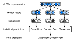
Figure 2: The morphological features prediction.

For each attribute its value is predicted with a fully connected network with one hidden layer and soft-max activation function. Various words are defined by the sets of various morphological features. Since for each word only some attributes are present in the set of morphological features, the possible values are extended with “not applicable” label. It allows the model to learn that an attribute is not present in the set of morphological features of a particular word.

2.3 Lemmatizer

Lemmatizer takes two different inputs. First, features extracted by the biLSTM encoder are used, however their dimensionality is reduced with a single fully connected layer. Next, the word, for which we want to predict a lemma, is converted to a sequence of characters. The special symbols “beginning-of-word” and “end-of-word” are added to the sequence to represent the beginning and the end of the word. Each character in the sequence is represented as a trainable embedding vector. The final input to the lemmatizer is a sequence of character embeddings concatenated with the reduced version of features extracted by the biLSTM encoder. Note that each character embedding is concatenated with exactly the same extracted feature vector.

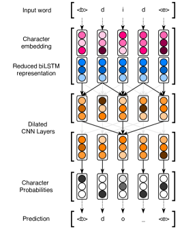
Figure 3: The lemmas prediction.

Then the dilated convolutional neural network followed by soft-max function converts given input to the sequence of probabilities of one-hot encoded characters of the predicted lemma (see Figure 3).

2.4 Parser

2.4.1 Arc Prediction

Two single fully connected layers transform features extracted by the biLSTM encoder into head and dependent vector representations. A fully connected dependency graph is defined with an adjacency matrix. The columns of the matrix correspond to heads represented with heads’ vector representations and the rows correspond to dependents represented with dependents’ vector representations. The elements of the adjacency matrix, in turn, are dot products of all pairs of the head and dependent vector representations. Soft-max function is then applied to each row of the matrix to predict the adjacent head-dependent pairs (see Figure 4).

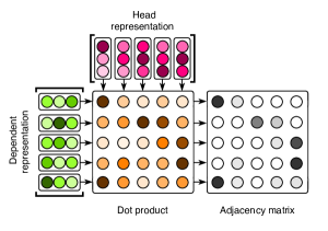
Figure 4: The adjacency matrix and the extracted dependency tree of the sentence The car is red.

2.4.2 Loss Function

In order to force the network to predict the correct head for each dependent and thus a correct dependency tree, the cross-entropy loss function is used for each row in the adjacency matrix. Note however that such formulation of the problem can lead the network to predict an adjacency matrix with cycles.

We aim to get an adjacency matrix for which a simple greedy algorithm would suffice to construct the correct tree. Therefore, we propose an additional ‘cycle-penalty’ loss function which reduces the number of cycles in the predicted adjacency matrix:

$$\mathrm{loss}(A)=\sum^{K}_{k=1}\mathrm{tr}(A^{k})$$

The non-zero trace of $A^{k}$ indicates that there are the paths of the length $k$ in the graph represented by the adjacency matrix $A$ Norman (1965). Therefore, by minimizing the sum of the traces of the subsequent powers of $A$ we reduce the number of cycles in the predicted graph. In an ideal scenario $K$ should be equal to the length of the sentence, but in practice even $K=3$ helps to reduce the number of cycles. The final loss used to train the arc prediction model is a sum of cross-entropy loss and ‘cycle-penalty’ loss.

If the smoothed adjacent matrix still contains cycles, Chu-Liu-Edmonds algorithm Chu and Liu (1965); Edmonds (1967) is applied to extract the properly built dependency tree in the final step of the prediction procedure.

2.4.3 Label Prediction

In order to predict the label for each arc of the predicted dependency tree, the vector representations of the arc’s head and its dependent are calculated. These representations do not correspond to those used during the arc prediction, but they are obtained in a similar way. The estimated vector of the dependent is concatenated with the weighted average of its predicted head vector. The weights correspond to probabilities of a word being the dependent’s head predicted by the arc model described in the previous section. It is not possible to take just the vector of a single predicted head, because it would prevent the model to be trained together with the rest of the system, as argmax operation is not differentiable. The concatenated vector representations are then fed to a single fully connected layer with soft-max activation function.

3 Implementation Details

3.1 Network Hyperparameters

Word Embedding

We use 300-dimensional fastText word embeddings Grave et al. (2018), which are then converted to 100-dimensional vectors by a single fully connected layer. The embedding is not available for some languages, i.e. for Old Church Slavonic (‘cu_proiel’), Old French (‘fro_srcmf’), Gothic (‘got_proiel’), Kurmanji (‘kmr_mg’), North Sámi (‘sme_giella’) or it seems incorrect, i.e. in Slovak (‘sk_snk’). Therefore, we estimate the embedding for these languages during the training of the whole system.

Character Embedding

The character level embedding is calculated with three convolutional layers with 512, 128 and 64 filters with dilation rates equal to 1, 2 and 4. All of the filters have the kernel of size 3. The input character embedding has the size of 64.

Final Word Embedding

The final word embedding is the concatenation of the 100-dimensional word embedding and the 64-dimensional character-based word embedding. It has thus 164 dimensions.

Feature Extraction

Two biLSTM layers with 512 hidden units are used to extract the final features.

Tagger

The tagger uses a fully connected network with the hidden layer of the size 64. The model to predict morphological features uses the hidden layer of 128 neurons.

Lemmatizer

The lemmatizer uses three convolutional layers with 256 filters and dilation rates equal to 1, 2 and 4. All of the filters have the kernel of size 3. Then the final convolutional layer with the kernel size equal to 1 is used to predict lemmas. The input characters, represented as the embeddings with 256 dimensions, are concatenated with the features extracted with the biLSTM encoder and reduced to 32 dimensions with a single fully connected layer.

Parser

The arc model uses heads’ and dependents’ vector representations with 512 dimensions. The labelling model uses 128-dimensional vectors.

All fully connected layers use tanh activation function and all convolutional layers use rectified linear unit (ReLU, Nair and Hinton, 2010).

3.2 Regularization

We apply both Gaussian Dropout (with the dropout rate of 0.25) and Gaussian Noise (with the standard deviation on 0.2) to the final word embedding and after processing each biLSTM layer. All fully connected layers use the standard dropout Srivastava et al. (2014) with the dropout rate of 0.25. The biLSTM layers use both the standard and recurrent dropout with the rate of 0.25. Moreover, the biLSTM and convolutional layers use L2 regularization with the rate of $1\times 10^{-6}$ and the trainable embeddings use L2 regularization with the rate of $1\times 10^{-5}$.

3.3 Training

We use cross-entropy loss for all parts of the system. The loss for the arc prediction model is a sum of cross-entropy loss and novel loss (see Section 2.4.2). The final loss is the weighted sum of losses with the following weights for each task:

• 0.05 for part-of-speech tagging,

• 0.2 for morphological features prediction,

• 0.05 for lemmatization,

• 0.2 for arc prediction,

• 0.8 for label prediction.

The whole system is optimized with ADAM Kingma and Ba (2014) with the learning rate equal to $0.002$ and $\beta_{1}=\beta_{2}=0.9$. Typically, the batch size of approximately 2500 words is used, however for a few of the smallest treebanks the batch size is reduced to 1000 or even 75 words. Each batch consists of sentences with a similar length, but the ordering of batches is randomized within each epoch. Each observation (i.e. sentence) is weighted with the log of the sentence length that forces the model to focus on longer (and usually more difficult) sentences. The model is trained for maximum of 400 epochs and the learning rate is reduced twice by the factor of two when the validation score reaches plateau. For languages with multiple treebanks, first a general model is trained on all sentences from these treebanks and then the model is fine-tuned for each treebank.

3.4 Self-training

For 20 arbitrarily selected treebanks, mostly the smallest ones, self-training method Triguero et al. (2015) is used to increase the performance of the system. First the model is trained in a standard way, as described in the previous sections. Then the ‘semi-supervised’ training set is built. It contains sentences with the total of approximately 25M words taken from raw data provided by CoNLL 2018 organizers. For Uyghur language only 3M words are available. The provided data sets come either from Wikipedia or Commom Crawl. Where it is possible we choose the sentences from Common Crawl, due to longer (on average) sentence sizes. The pre-trained model is then used to predict dependency trees, lemmas and part-of-speech tags for all sentences in the ‘semi-supervised’ training set. Finally, the new model is trained on this ‘semi-supervised’ training set for only one epoch and fine-tuned on the gold-standard training data, using the standard training procedure.

3.5 Languages with No Resources

Our solution for processing treebanks with no training data is very simple. We choose another language for which training data is available and train the model on this data. The estimated model is used for predictions in the language with no training data. We use the following treebank pairs:

• ‘br_keb’ (Breton) – ‘ga_idt’ (Irish),

• ‘fo_oft’ (Faroese) – ‘no_nynorsk’ (Norwegian),

• ‘pcm_nsc’ (Naija) – ‘en_ewt’ (English),

• ‘th_pud’ (Thai) – ‘vi_vtb’ (Vietnamese).

The parallel UD treebanks for Czech, English, Finish, and Swedish, and the treebank for modern Japanese are processed with the models estimated on other treebanks for the respective languages:

• ‘cs_pud’ – ‘cs_pdt’ (Czech),

• ‘en_pud’ – ‘en_ewt’ (English),

• ‘fi_pud’ – ‘fi_tdt’ (Finish),

• ‘sv_pud’ – ‘sv_talbanken’ (Swedish),

• ‘ja_modern’ – ‘ja_gsd’ (Japanese).

4 Results

4.1 Overview

In the official evaluation Zeman et al. (2018) our system ranks 3th/4th for all three main metrics (ex aequo with LATTICE and UDPipe Future for LAS). It performs particularly well on small treebanks with no development data, but a reasonable size of the training set. For example, the system ranks 1st in terms of all three measures on Russian ‘ru_taiga’ treebank, 1st (MLAS and BLEX) and 2nd (LAS) on Latin ‘la_perseus’ treebank and spoken Slovenian ‘sl_sst’ treebank, and 1st (MLAS and BLEX) and 3rd (LAS) on spoken Norwegian ‘no_nynorsklia’ treebank. It is worth noting that overall MLAS and BLEX scores obtained by our system trained on small treebanks are currently the state of the art (see Table 1). With respect to LAS score, our system ranks 3rd.

Category	LAS	MLAS	BLEX
All	73.02	60.25	64.44
Big	81.72	70.30	74.42
PUD	72.18	58.07	60.97
Small	66.90	49.24	54.89
Low-resource	19.26	1.89	6.17

Table 1: Official results of our system in CoNLL shared task. State-of-the-art results are in bold.

Regarding to processing big treebanks, our system performs very well on Czech ‘cs_fictree’ treebank and English ‘en_gum’ treebank (1st place in MLAS and BLEX, and 2nd place in LAS), and Latin ‘la_ittb’ treebank (1st place in MLAS and BLEX, and 3rd place in LAS). It is very important to note that most of the mentioned languages, i.e. Russian, Latin, Slovenian, Norwegian, and Czech, are Indo-European languages (fusional). Furthermore, for other fusional languages, e.g. Galician, Ancient Greek, Polish, Ukrainian, Dutch, Swedish, French, Italian, Spanish, Basque, our system provides quite satisfying results as well. It follows that our system is especially appropriate for processing fusional languages.

Our last observation concerns the usefulness of external word embeddings for NLP system with a neural architecture. The languages without external word embeddings (see Section 3.1) are processed by our system significantly below its overall performance. Hence, the external word embeddings are crucial for a neural NLP system.

4.2 Impact of Loss Function

For 15 arbitrarily selected treebanks we train the models without the additional loss function and we compare UAS scores of these models with UAS scores obtained by the models estimated with the additional loss function (with $K=3$, see Section 2.4.2). Moreover for each treebank we calculate what would be the fraction of trees with cycles if we use the greedy algorithm to construct the predicted trees.

Note that the following results cannot be directly compared to the official test results. First we report the scores on the validation set. Second we use the gold-standard segmentation instead of the segmentation predicted by the baseline model.

Treebank	UAS		% Cycles
	without	with	without	with
ar_padt	86.23	86.39	7.70	4.51
bg_btb	92.32	92.45	1.26	1.52
cu_proiel	86.94	86.49	4.19	3.91
da_ddt	86.61	86.24	5.14	4.61
de_gsd	87.74	87.64	3.50	2.63
es_ancora	92.39	92.49	3.08	3.39
fa_seraji	90.30	90.44	5.18	4.51
got_proiel	83.88	83.57	5.48	4.57
hr_set	90.34	90.50	6.71	4.95
hu_szeged	81.99	82.48	11.34	9.75
id_gsd	84.33	84.47	6.98	6.98
lv_lvtb	85.69	85.58	6.28	4.66
pt_bosque	92.65	92.63	1.25	1.43
ro_rrt	91.04	90.89	2.39	2.53
vi_vtb	68.92	69.02	15.00	12.63
Average	86.76	86.75	5.70	4.84

Table 2: Comparison of the models trained with and without the additional loss function.

The additional loss only slightly decreases UAS (see the second and the third column in Table 2). However, it also has only a small impact on the cycles reduction (see the fourth and the fifth column in Table 2). If there is a lot of cycles in the graphs predicted without the additional loss, e.g. 7.7% cycles in ‘ar_padt’ (Arabic), the number of cycles is significantly reduced with the additional loss function, i.e. the reduction by 3.2 p.p. If the rate of cycles is lower, e.g. 4.19% in ‘cu_proiel’ (Old Church Slavonic), fewer cycles are corrected, i.e. the reduction by 0.28 p.p. Finally, there are four treebanks – ‘bg_btb’ (Bulgarian), ‘es_ancora’ (Spanish), ‘pt_bosque’ (Portuguese), and ‘ro_rrt’ (Romanian), for which the additional loss function slightly increases the number of cycles.

4.3 Impact of Self-training

We test the impact of self-training method on the performance of the system trained on 20 selected treebanks. Again the models are tested on the validation set with the gold-standard segmentation.

Treebank	LAS		MLAS		BLEX
	std	self	std	self	std	self
bg_btb	88.84	89.23	79.39	80.12	78.89	79.21
da_ddt	83.24	84.89	72.40	75.76	76.73	78.93
el_gdt	87.89	89.19	73.55	76.98	74.06	77.30
eu_bdt	81.58	82.85	65.94	68.15	76.29	77.49
fa_seraji	86.91	87.22	80.19	81.18	80.86	81.36
ga_idt	N/A	N/A	N/A	N/A	N/A	N/A
he_htb	84.39	85.60	71.31	73.63	73.87	75.34
hr_set	86.06	86.22	71.17	71.61	79.01	79.38
hu_szeged	77.39	80.55	60.77	67.28	70.55	74.41
id_gsd	77.62	77.97	64.27	66.22	74.03	74.62
kk_ktb	N/A	N/A	N/A	N/A	N/A	N/A
lv_lvtb	80.52	82.67	65.53	69.11	71.71	74.19
ro_rrt	85.88	86.68	76.49	77.57	79.47	80.39
sk_snk	83.44	85.52	56.05	66.69	72.77	77.13
tr_imst	64.07	64.95	49.26	51.97	57.15	58.87
ug_udt	63.89	65.50	38.21	41.83	51.48	53.89
uk_iu	85.83	87.91	68.35	73.69	78.35	81.65
ur_udtb	80.91	81.34	52.92	53.48	71.09	71.72
vi_vtb	58.82	60.52	49.29	51.87	54.85	56.93
zh_gsd	77.09	76.71	65.17	64.88	69.68	68.93
Average	79.69	80.86	64.46	67.33	71.71	73.43

Table 3: Comparison of the standard (std) and self-training (self) models on the validation set using the gold-standard segmentation. Note that ‘kk_ktb’ (Kazakh) and ‘ga_idt’ (modern Irish) treebanks do not have validation sets, so we are unable to report any results.

Comparing the results of the models estimated on training data with the results of the models estimated with the self-training method (see Table 3), we notice that self-training significantly increases the performance of the system. There is an increase for all metrics for all treebanks except for ‘zh_gsd’ (Chinese). On average there is an increase of 1.2 p.p. for LAS, 2.9 p.p. for MLAS and 1.7 p.p. for BLEX.

5 Conclusion

We described the ICS PAS system which took part in CoNLL 2018 shared task. Our goal was to build one system for preprocessing natural languages, i.e. for part-of-speech tagging, lemmatisation and dependency parsing. The three system’s modules – tagger, lemmatizer and parser – are jointly trained. The proposed neural system ranks 3th/4th in the official evaluation of the shared task. It is worth nothing that the system is especially useful for estimating the models on relative sparse data (small treebanks), as it overcame other systems in terms of MLAS and BLEX. Furthermore, our system is especially appropriate for processing Indo-European fusional languages.

The self-training procedure significantly increases the performance of the system. The proposed loss function, in turn, has only a slight impact on the cycles reduction and UAS scores. The external word embeddings are crucial for our neural-based system.

References

- Buchholz and Marsi (2006) Sabine Buchholz and Erwin Marsi. 2006. CoNLL-X shared task on Multilingual Dependency Parsing. In Proceedings of the Tenth Conference on Computational Natural Language Learning. pages 149–164.
- Chu and Liu (1965) Yoeng Jin Chu and Tseng Hong Liu. 1965. On the Shortest Arborescence of a Directed Graph. Science Sinica 14:1396–1400.
- Edmonds (1967) Jack Edmonds. 1967. Optimum Branchings. Journal of Research of the National Bureau of Standards 71B(4):233–240.
- Grave et al. (2018) Edouard Grave, Piotr Bojanowski, Prakhar Gupta, Armand Joulin, and Tomas Mikolov. 2018. Learning word vectors for 157 languages. In Proceedings of the International Conference on Language Resources and Evaluation (LREC 2018).
- Graves and Schmidhuber (2005) Alex Graves and Jürgen Schmidhuber. 2005. Framewise Phoneme Classification with Bidirectional LSTM and Other Neural Network Architectures. Neural Networks 18(5):602–610.
- Hochreiter and Schmidhuber (1997) Sepp Hochreiter and Jürgen Schmidhuber. 1997. Long short-term memory. Neural Computation 9(8):1735–1780.
- Kingma and Ba (2014) Diederik P. Kingma and Jimmy Ba. 2014. Adam: A Method for Stochastic Optimization. CoRR abs/1412.6980. http://arxiv.org/abs/1412.6980.
- Nair and Hinton (2010) Vinod Nair and Geoffrey E. Hinton. 2010. Rectified Linear Units Improve Restricted Boltzmann Machines. In Proceedings of ICML’10, pages 807–814.
- Nivre et al. (2018) Joakim Nivre, Mitchell Abrams, Željko Agić, Lars Ahrenberg, Lene Antonsen, Maria Jesus Aranzabe, Gashaw Arutie, Masayuki Asahara, Luma Ateyah, Mohammed Attia, Aitziber Atutxa, Liesbeth Augustinus, Elena Badmaeva, Miguel Ballesteros, Esha Banerjee, Sebastian Bank, Verginica Barbu Mititelu, John Bauer, Sandra Bellato, Kepa Bengoetxea, Riyaz Ahmad Bhat, Erica Biagetti, Eckhard Bick, Rogier Blokland, Victoria Bobicev, Carl Börstell, Cristina Bosco, Gosse Bouma, Sam Bowman, Adriane Boyd, Aljoscha Burchardt, Marie Candito, Bernard Caron, Gauthier Caron, Gülşen Cebiroğlu Eryiğit, Giuseppe G. A. Celano, Savas Cetin, Fabricio Chalub, Jinho Choi, Yongseok Cho, Jayeol Chun, Silvie Cinková, Aurélie Collomb, Çağrı Çöltekin, Miriam Connor, Marine Courtin, Elizabeth Davidson, Marie-Catherine de Marneffe, Valeria de Paiva, Arantza Diaz de Ilarraza, Carly Dickerson, Peter Dirix, Kaja Dobrovoljc, Timothy Dozat, Kira Droganova, Puneet Dwivedi, Marhaba Eli, Ali Elkahky, Binyam Ephrem, Tomaž Erjavec, Aline Etienne, Richárd Farkas, Hector Fernandez Alcalde, Jennifer Foster, Cláudia Freitas, Katarína Gajdošová, Daniel Galbraith, Marcos Garcia, Moa Gärdenfors, Kim Gerdes, Filip Ginter, Iakes Goenaga, Koldo Gojenola, Memduh Gökırmak, Yoav Goldberg, Xavier Gómez Guinovart, Berta Gonzáles Saavedra, Matias Grioni, Normunds Grūzītis, Bruno Guillaume, Céline Guillot-Barbance, Nizar Habash, Jan Hajič, Jan Hajič jr., Linh Hà Mỹ, Na-Rae Han, Kim Harris, Dag Haug, Barbora Hladká, Jaroslava Hlaváčová, Florinel Hociung, Petter Hohle, Jena Hwang, Radu Ion, Elena Irimia, Tomáš Jelínek, Anders Johannsen, Fredrik Jørgensen, Hüner Kaşıkara, Sylvain Kahane, Hiroshi Kanayama, Jenna Kanerva, Tolga Kayadelen, Václava Kettnerová, Jesse Kirchner, Natalia Kotsyba, Simon Krek, Sookyoung Kwak, Veronika Laippala, Lorenzo Lambertino, Tatiana Lando, Septina Dian Larasati, Alexei Lavrentiev, John Lee, Phuong Lê Hông, Alessandro Lenci, Saran Lertpradit, Herman Leung, Cheuk Ying Li, Josie Li, Keying Li, KyungTae Lim, Nikola Ljubešić, Olga Loginova, Olga Lyashevskaya, Teresa Lynn, Vivien Macketanz, Aibek Makazhanov, Michael Mandl, Christopher Manning, Ruli Manurung, Cătălina Mărănduc, David Mareček, Katrin Marheinecke, Héctor Martínez Alonso, André Martins, Jan Mašek, Yuji Matsumoto, Ryan McDonald, Gustavo Mendonça, Niko Miekka, Anna Missilä, Cătălin Mititelu, Yusuke Miyao, Simonetta Montemagni, Amir More, Laura Moreno Romero, Shinsuke Mori, Bjartur Mortensen, Bohdan Moskalevskyi, Kadri Muischnek, Yugo Murawaki, Kaili Müürisep, Pinkey Nainwani, Juan Ignacio Navarro Horñiacek, Anna Nedoluzhko, Gunta Nešpore-Bērzkalne, Luong Nguyên Thị, Huyên Nguyên Thị Minh, Vitaly Nikolaev, Rattima Nitisaroj, Hanna Nurmi, Stina Ojala, Adédayọ̀ Olúòkun, Mai Omura, Petya Osenova, Robert Östling, Lilja Øvrelid, Niko Partanen, Elena Pascual, Marco Passarotti, Agnieszka Patejuk, Siyao Peng, Cenel-Augusto Perez, Guy Perrier, Slav Petrov, Jussi Piitulainen, Emily Pitler, Barbara Plank, Thierry Poibeau, Martin Popel, Lauma Pretkalniņa, Sophie Prévost, Prokopis Prokopidis, Adam Przepiórkowski, Tiina Puolakainen, Sampo Pyysalo, Andriela Rääbis, Alexandre Rademaker, Loganathan Ramasamy, Taraka Rama, Carlos Ramisch, Vinit Ravishankar, Livy Real, Siva Reddy, Georg Rehm, Michael Rießler, Larissa Rinaldi, Laura Rituma, Luisa Rocha, Mykhailo Romanenko, Rudolf Rosa, Davide Rovati, Valentin Roșca, Olga Rudina, Shoval Sadde, Shadi Saleh, Tanja Samardžić, Stephanie Samson, Manuela Sanguinetti, Baiba Saulīte, Yanin Sawanakunanon, Nathan Schneider, Sebastian Schuster, Djamé Seddah, Wolfgang Seeker, Mojgan Seraji, Mo Shen, Atsuko Shimada, Muh Shohibussirri, Dmitry Sichinava, Natalia Silveira, Maria Simi, Radu Simionescu, Katalin Simkó, Mária Šimková, Kiril Simov, Aaron Smith, Isabela Soares-Bastos, Antonio Stella, Milan Straka, Jana Strnadová, Alane Suhr, Umut Sulubacak, Zsolt Szántó, Dima Taji, Yuta Takahashi, Takaaki Tanaka, Isabelle Tellier, Trond Trosterud, Anna Trukhina, Reut Tsarfaty, Francis Tyers, Sumire Uematsu, Zdeňka Urešová, Larraitz Uria, Hans Uszkoreit, Sowmya Vajjala, Daniel van Niekerk, Gertjan van Noord, Viktor Varga, Veronika Vincze, Lars Wallin, Jonathan North Washington, Seyi Williams, Mats Wirén, Tsegay Woldemariam, Tak-sum Wong, Chunxiao Yan, Marat M. Yavrumyan, Zhuoran Yu, Zdeněk Žabokrtský, Amir Zeldes, Daniel Zeman, Manying Zhang, and Hanzhi Zhu. 2018. Universal Dependencies 2.2. LINDAT/CLARIN digital library at the Institute of Formal and Applied Linguistics (ÚFAL), Faculty of Mathematics and Physics, Charles University. http://hdl.handle.net/11234/1-2837.
- Nivre et al. (2016) Joakim Nivre, Marie-Catherine de Marneffe, Filip Ginter, Yoav Goldberg, Jan Hajič, Christopher D. Manning, Ryan T. McDonald, Slav Petrov, Sampo Pyysalo, Natalia Silveira, Reut Tsarfaty, and Daniel Zeman. 2016. Universal Dependencies v1: A Multilingual Treebank Collection. In Proceedings of the Tenth International Conference on Language Resources and Evaluation LREC 2016. pages 1659–1666.
- Nivre et al. (2007) Joakim Nivre, Johan Hall, Sandra Kübler, Ryan McDonald, Jens Nilsson, Sebastian Riedel, and Deniz Yuret. 2007. The CoNLL 2007 Shared Task on Dependency Parsing. In Proceedings of the CoNLL Shared Task Session of EMNLP-CoNLL 2007. pages 915–932.
- Norman (1965) R. L. Norman. 1965. A matrix method for location of cycles of a directed graph. AIChE Journal 11(3):450–452. https://doi.org/10.1002/aic.690110316.
- Srivastava et al. (2014) Nitish Srivastava, Geoffrey Hinton, Alex Krizhevsky, Ilya Sutskever, and Ruslan Salakhutdinov. 2014. Dropout: A simple way to prevent neural networks from overfitting. Journal of Machine Learning Research 15:1929–1958. http://jmlr.org/papers/v15/srivastava14a.html.
- Straka and Straková (2017) Milan Straka and Jana Straková. 2017. Tokenizing, POS Tagging, Lemmatizing and Parsing UD 2.0 with UDPipe. In Proceedings of the CoNLL 2017 Shared Task: Multilingual Parsing from Raw Text to Universal Dependencies. Association for Computational Linguistics, Vancouver, Canada, pages 88–99. http://www.aclweb.org/anthology/K/K17/K17-3009.pdf.
- Triguero et al. (2015) Isaac Triguero, Salvador García, and Francisco Herrera. 2015. Self-labeled techniques for semi-supervised learning: taxonomy, software and empirical study. Knowledge and Information Systems 42:245–284. https://doi.org/https://doi.org/10.1007/s10115-013-0706-y.
- Yu and Koltun (2016) Fisher Yu and Vladlen Koltun. 2016. Multi-Scale Context Aggregation by Dilated Convolutions. CoRR abs/1511.07122. http://arxiv.org/abs/1511.07122.
- Zeman et al. (2018) Daniel Zeman, Jan Hajič, Martin Popel, Martin Potthast, Milan Straka, Filip Ginter, Joakim Nivre, and Slav Petrov. 2018. CoNLL 2018 Shared Task: Multilingual Parsing from Raw Text to Universal Dependencies. In Proceedings of the CoNLL 2018 Shared Task: Multilingual Parsing from Raw Text to Universal Dependencies. Association for Computational Linguistics, Brussels, Belgium, pages 1–20.
- Zeman et al. (2017) Daniel Zeman, Martin Popel, Milan Straka, Jan Hajič, Joakim Nivre, Filip Ginter, Juhani Luotolahti, Sampo Pyysalo, Slav Petrov, Martin Potthast, Francis Tyers, Elena Badmaeva, Memduh Gökırmak, Anna Nedoluzhko, Silvie Cinková, Jan Hajič jr., Jaroslava Hlaváčová, Václava Kettnerová, Zdenka Urešová, Jenna Kanerva, Stina Ojala, Anna Missilä, Christopher D. Manning, Sebastian Schuster, Siva Reddy, Dima Taji, Nizar Habash, Herman Leung, Marie-Catherine de Marneffe, Manuela Sanguinetti, Maria Simi, Hiroshi Kanayama, Valeria dePaiva, Kira Droganova, Héctor Martínez Alonso, Çağrı Çöltekin, Umut Sulubacak, Hans Uszkoreit, Vivien Macketanz, Aljoscha Burchardt, Kim Harris, Katrin Marheinecke, Georg Rehm, Tolga Kayadelen, Mohammed Attia, Ali Elkahky, Zhuoran Yu, Emily Pitler, Saran Lertpradit, Michael Mandl, Jesse Kirchner, Hector Fernandez Alcalde, Jana Strnadová, Esha Banerjee, Ruli Manurung, Antonio Stella, Atsuko Shimada, Sookyoung Kwak, Gustavo Mendonça, Tatiana Lando, Rattima Nitisaroj, and Josie Li. 2017. CoNLL 2017 Shared Task: Multilingual Parsing from Raw Text to Universal Dependencies. In Proceedings of the CoNLL 2017 Shared Task: Multilingual Parsing from Raw Text to Universal Dependencies. Association for Computational Linguistics, pages 1–19. http://www.aclweb.org/anthology/K/K17/K17-3001.pdf.