Abstract

In this paper, we explore the potential of the LHC to measure the rate of $\mathrm{p}\mathrm{p}\rightarrow\mathrm{p}~{}WW\gamma~{}\mathrm{p}$ process, also to probe the new effective couplings contributing to the $WW\gamma$ and $WW\gamma\gamma$ vertices. The analysis is performed at the $\sqrt{s}=13$ TeV, in the di-leptonic decay channel, and assuming 300 $\,{\rm fb}^{-1}$ integrated luminosity (IL). In addition to the presence of two opposite sign leptons, a photon, and missing energy, the distinctive signature of this process is the presence of two intact protons flying few millimeters from the initial beam direction in both sides of interaction points which suppress the background process effectively. To exploit this feature of signal we benefit from forward detectors (FDs) placed about 200 meters from the interaction point to register the kinematics of tagged protons. In order to overcome the major sources of backgrounds, we introduced three categories of selection cuts dealing with objects that strike the central detector, protons hitting the FDs, and correlations of central objects and protons, respectively. We also evaluate the probability of pile-up protons to be tagged in the FDs as a function of the mean number of pile-up. Then the sensitivity of the LHC to observe this process and constraints on multi-boson effective couplings are extracted. The obtained expected limits show very good improvements for dimension-8 quartic couplings and competitive bounds on dimension-6 anomalous triple couplings w.r.t the current experimental limits. Therefore, we propose this process to the LHC experiments as a sensitive and complementary channel to study the multi-gauge boson couplings.

1 Introduction

In the standard model (SM) framework, the non-abelian property of $SU(2)_{L}\times U(1)_{Y}$ gauge theory predicts triple and quartic gauge boson self-interactions. The triple and quartic couplings are connected to electroweak symmetry breaking and explore the non-abelian gauge structure. Therefore, studying these couplings provides an important confirmation to the SM. Additionally, any deviation from the SM prediction of these gauge self-interactions could be a hint to beyond the SM. For instance, triple gauge boson couplings could be a consequence of integrating out of non-standard heavy particles at the loop level while the exchange of heavy new particles at tree level can contribute to quartic gauge couplings. As a result, any deviation from the SM predictions observed by the current experimental precision might appear at quartic rather than triple gauge couplings. From the theoretical point of view, such deviations can be explained in the effective field theory framework with high-dimensional model-independent operators that modify the self-interaction of electroweak gauge bosons or lead to new vertices both known as anomalous couplings [1]. The anomalous triple gauge couplings (aTGCs) and anomalous quartic gauge couplings (aQGCs) can be parametrized with dimension-6 [3, 2] and dimension-8 operators [4].

The direct probe of triple and quartic gauge boson interactions could be achieved by measurements of multi-boson productions at the colliders that have been carried out both in the experimental measurements and phenomenological studies. For instance, the observed bounds on aTGCs have been obtained from $WW$ production at LEP with center-of-mass energies $\sqrt{s}=130-209{\rm\ GeV}$[5] which is also measured in leptonic final states at Tevatron [6]. Besides, $WZ$ production at semi-leptonic final state at Tevatron with $\sqrt{s}=1.96{\rm\ TeV}$ has been tested for aTGCs [7]. Recently, various measurements on the di-boson production such as $WW$,$WZ$ and $W\gamma$ are performed at the LHC with $\sqrt{s}=7,8{\rm\ TeV}$ [9, 8, 10, 11], also the same final state in one of the W boson decaying leptonicly and the other W or Z boson decaying hadronically has been explored at $\sqrt{s}=13{\rm\ TeV}$ [12, 13, 14, 15]. The observed limits on aQGCs in the context of dimension-8 are available from exclusive $W$ pair production at Tevatron [16]. The constraints on aQGCs at the LHC for same sign W pair production plus two jets in leptonic decay of $W$ bosons at $\sqrt{s}=8{\rm\ TeV}$ [17] and $WV\gamma$ production with $V=W,Z$ following by semi-leptonic decay of massive gauge bosons at the same center-of-mass energy [18] have been obtained. Furthermore, there are many phenomenological studies at lepton colliders such as $e^{-}e^{+}$ [19, 20, 21, 25, 22, 23, 24, 26, 27, 28, 30, 29, 31, 32] and hadron colliders [40, 33, 34, 35, 36, 37, 38, 39, 41] in which the potential to probe multi-gauge boson couplings have been explored. Beside direct constraints, indirect searches on aTGCs have been performed using the data from rare B-meson decays [42], as well as coupling measurements of Higgs boson to electroweak gauge boson at Tevatron and LHC [43, 44, 45]. An alternative possibility to explore the multi-gauge boson couplings is via the central exclusive production (CEP) at the LHC. The CEP happens through the exchange of two color-singlet states radiated from two crossing protons resulting in an isolated central system and two intact protons that fly in the very forward-backward regions of the interaction point. Benefiting from FDs such as CMS-TOTEM Precision Proton Spectrometer (CT-PPS)[46] and ATLAS Forward Proton (AFP) [47] these two protons can be tagged and consequently, CEP could be distinguished from inclusive background processes. Therefore, exploring CEP processes can provide a unique window to search for new physics namely anomalous gauge couplings. The detailed analysis of central exclusive processes with $W$ boson pair production including aTGCs and aQGCs have been performed at Tevatron [16]. Moreover, observed bounds on dimension-6 and -8 operators via central exclusive $WW$ production at $\sqrt{s}=7{\rm\ TeV}$, $8{\rm\ TeV}$, and their combinations without proton tagging are reported by CMS and ATLAS experiments [50, 48, 49]. Additionally, several phenomenological studies estimated the potential of the LHC for CEP processes to probe the anomalous gauge boson couplings that can be found in Refs [51, 52, 39, 53, 54]. In this paper, we propose $WW\gamma$ production via the CEP as a new channel at the LHC and explore the potential of this process to probe aTGCs and aQGCs. This process is purely sensitive to gauge boson couplings and can be a complementary channel to increase the sensitivity to the SM and anomalous $WW\gamma$ and $WW\gamma\gamma$ couplings. We consider the fully leptonic decay of W bosons and $300\,{\rm fb}^{-1}$ of proton-proton collision data at the center-of-mass energy of $13{\rm\ TeV}$. The paper is organized as follows: In section 2, a general description of the flux of emitted photon from a proton is provided. Section 3 gives a short review of the effective field theory approach for anomalous gauge couplings. In section 4 the CEP of $WW\gamma$ at the LHC is explained. In Section 5 the strategy of analysis to the optimum selection of signal and suppression of different sources of backgrounds are described. Section 6 describes the potential of the LHC to measure the SM $WW\gamma$ process via photon-photon scattering. In section 7 the expected limits on aTGCs and aQGCs are explained. Finally, in section 8 the summary and conclusion are provided.

2 Photon-photon interaction at the LHC

Photon-photon interactions at the LHC can be studied through the CEP that is defined as

$$\mathrm{p}\mathrm{p}\rightarrow\mathrm{p}\oplus X\oplus\mathrm{p}.$$ (1)

In these type of processes two incoming protons are collided via exchange of two color-singlet states such as photons and they remain intact. The amount of missing energy of each proton which is carried by each photon, produce state $X$ which can be detected at the central detectors while the two unbroken protons fly in the forward and backward regions of the central detector with very small angle w.r.t their original directions. Therefore, one sees the large rapidity gaps ($\oplus$) among the centrally produced state and two forward protons which is one of the distinctive signatures of the CEP processes.

Despite the fact that the cross sections of the CEP processes are small w.r.t parton-parton initial state processes, they can be measured accurately in a very clean environment due to several reasons. For instance, due to the absence of proton remnants, one could obtain the clean experimental environment like electron-positron colliders. Unlike the usual hard proton-proton scattering, by measuring the fractional energy loss of each proton ($\xi_{1},\xi_{2}$) which is defined as $\xi=\frac{E_{\mathrm{p}}-E_{\mathrm{p^{\prime}}}}{E_{\mathrm{p}}}$ ($E_{\mathrm{p}}$ and $E_{\mathrm{p^{\prime}}}$ are energy of incoming and outgoing protons, respectively) the scale of collision can be determined event-by-event basis. Also measurement of the forward protons permits to predict the kinematics of centrally produced state and matching them can lead to several orders of magnitude suppression in the background processes. Benefiting from these properties which FDs granted us, the CEP could provide a rich testing ground for electroweak and QCD sector of the SM and unique window to physics beyond the SM.

The cross section of the CEP process when two photons exchange, can be computed in the framework of the Equivalent Photon Approximation (EPA)[55, 56, 57]. In this approximation the cross section can be factorized as following

$$\mathrm{d}\sigma(\mathrm{p}\mathrm{p}\rightarrow\mathrm{p}X\mathrm{p})=\hat{\sigma}(\gamma\gamma\rightarrow X)\mathrm{d}N_{1}^{\gamma}\mathrm{d}N_{2}^{\gamma},$$ (2)

where $\hat{\sigma}(\gamma\gamma\rightarrow X)$ is the Born cross section of state X and $dN^{\gamma}$ is the number of emitted photons with virtuality $Q^{2}$ and energy $E_{\gamma}$. Then the photon spectrum is given by:

$$\mathrm{d}^{2}N^{\gamma}=\frac{\alpha_{\text{em}}}{\pi}\frac{\mathrm{d}E_{\gamma}}{E_{\gamma}}\frac{\mathrm{d}Q^{2}}{Q^{2}}\left[\left(1-\frac{2E_{\gamma}}{\sqrt{s}}\right)\left(1-\frac{Q^{2}_{\text{min}}}{Q^{2}}\right)F_{E}+\frac{2E_{\gamma}^{2}}{s}F_{M}\right],$$ (3)

where $\alpha_{\text{em}}$ is fine structure constant and $\sqrt{s}$ is the center-of-mass energy of the proton-proton system and $m_{\mathrm{p}}$ is proton mass. The minimum allowed photon virtuality $Q_{\text{min}}$, $F_{\text{E}}$, and $F_{\text{M}}$ are defined respectively as

$$Q_{\text{min}}^{2}\equiv m_{\mathrm{p}}^{2}E_{\gamma}^{2}/[(s-\sqrt{s}E_{\gamma})],~{}F_{\text{M}}=G^{2}_{\text{M}},~{}F_{E}=\frac{(4m_{\mathrm{p}}^{2}G^{2}_{E}+Q^{2}G^{2}_{\text{M}})}{(4m_{\mathrm{p}}^{2}+Q^{2})}\,,$$ (4)

and $F_{\text{E}}$ and $F_{\text{M}}$ are functions of the electric ($G_{\text{E}}$) and magnetic ($G_{\text{M}}$) proton form factors. In the dipole approximation [39]

$$G^{2}_{\text{E}}=G^{2}_{\text{M}}/\mu_{\mathrm{p}}^{2}=(1+Q^{2}/Q^{2}_{0})^{-4},$$ (5)

the values of $Q^{2}_{0}$ and magnetic moment of protons are $0.71{\rm\ GeV}^{2}$ and $7.78$, respectively. Therefore, the flux of photon can be obtained by integrating over photon virtuality as follows

$$f(E_{\gamma})=\int^{Q^{2}_{\text{max}}}_{Q^{2}_{\text{min}}}\frac{\mathrm{d}^{2}N^{\gamma}}{\mathrm{d}E_{\gamma}\mathrm{d}Q^{2}}\mathrm{d}Q^{2},$$ (6)

where the value of $Q^{2}_{\text{max}}$ is set to large enough value 2-4 GeV². Thus, the total cross section can be obtained as a convolution of the effective photon fluxes and $\gamma\gamma\rightarrow X$ subprocess matrix elements as follows:

$$\frac{\mathrm{d}\sigma^{\gamma\gamma\rightarrow X}}{\mathrm{d}\Omega}=\int\frac{\mathrm{d}\sigma^{\gamma\gamma\rightarrow X}(W_{\text{miss}})}{\mathrm{d}\Omega}\frac{\mathrm{d}\mathcal{L}^{\gamma\gamma}}{\mathrm{d}W_{\text{miss}}}\mathrm{d}{W_{\text{miss}}}$$ (7)

where $\frac{\mathrm{d}\mathcal{L}^{\gamma\gamma}}{\mathrm{d}W_{\text{miss}}}$ is the two photons luminosity spectrum which can be obtained by integrating the product of two photon rates $f(E_{\gamma 1})f(E_{\gamma 2})$ over the energy of photons while the two photons invariant mass or equivalently total missing mass of protons $W_{\text{miss}}=2\sqrt{E_{\gamma 1}E_{\gamma 2}}=\sqrt{\xi_{1}\xi_{2}s}$ remains fix. Fig 1 shows the effective luminosity of two-photons in pp collision at $\sqrt{s}=13$ TeV as a function of invariant mass of two photons $W_{\text{miss}}$. The blue (solid) curve is the luminosity spectrum without any cut on the acceptance of FDs. The red (dashed) and green (dot-dashed) correspond to the $0.0015<\xi<0.2$ and $0.0015<\xi<0.5$ ranges of FDs acceptance [58, 59], respectively. As can be seen, the photon luminosity decrease by increasing the invariant mass of photons. Moreover, applying the lower cut on FDs acceptance leads to almost one order of magnitude drop in the photon luminosity at low invariant mass $W_{\text{miss}}$. However, the upper limits on FDs acceptance have little effect on the value of photon luminosity.

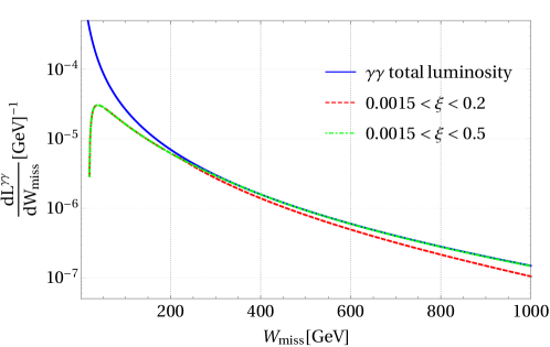
Figure 1: Photon-photon luminosity versus two-photon invariant mass at 13 TeV for total and FD acceptance.

The process that we would like to study is $W$-boson pair associated production with a photon in di-leptonic decay of $W$-bosons, generated through di-photon exchange. It is worth to mention that the process $\mathrm{p}\mathrm{p}\rightarrow W^{+}W^{-}\gamma$ has been measured at the LHC [60, 18]. In the following we briefly review the related effective Lagrangian to aTGCs and aQGCs.

3 EFT for anomalous gauge couplings involving photon

In this section, we focus on overall beyond the SM contributions to the triple and quartic gauge boson interactions. These contributions are described through effective field theory (EFT) approach in which the SM is extended by higher-dimensional operators composing by all possible combinations of the SM fields defined as

$$\mathcal{L}_{\text{EFT}}=\mathcal{L}_{\text{SM}}+\sum_{i}\frac{c_{i}^{(6)}}{\Lambda^{2}}\mathcal{O}_{i}^{(6)}+\sum_{j}\frac{c_{j}^{(8)}}{\Lambda^{4}}\mathcal{O}_{j}^{(8)}+...,$$ (8)

where $\Lambda$ is the mass scale of any new physics. The EFT is valid only for the energy $E\ll\Lambda$, $c_{i}$ are dimensionless Wilson coefficients and $\mathcal{O}_{i}^{(n)}$ represents the dimension $n$ operators. The operators respect the Lorentz symmetry and the SM gauge symmetry $SU(3)_{C}\times SU(2)_{L}\times U(1)_{Y}$. Only even-dimension operators can contribute if we require lepton and baryon number conservation. Therefore, the leading effective operators which give contribution to vertices containing multi-bosons are expected from dimension-6 operators. Gauge boson interactions within the EFT framework can be expressed as two nonlinear and linear approaches. In the nonlinear approach, the SM gauge symmetry is conserved and is realized by using the chiral Lagrangian parametrization given in Refs [32, 35]. In this approach triple and quartic gauge boson couplings appear as dimension-6 operators. In the linear approach, the SM gauge symmetry is broken by means of Higgs scalar doublet [32, 61]. In this parametrization, the quartic gauge boson couplings without triple gauge boson coupling appear as dimension-8 operators.
The general dimension-6 operators including a neutral vector boson and two charged vector bosons can be described by ten dimensionless couplings [62]. However, the number of operators can be decreased to 6 by imposing charge conjugate (C) and parity (P) invariant. The detail of operators is given in Ref. [62]. In this analysis for the ease of comparison to LEP results, we used the anomalous Lagrangian approach for triple gauge couplings which is known as LEP parametrization. The aTGCs defining the interaction of photon and W-bosons are expressed as:

$$\mathcal{L}_{WW\gamma}^{(6)}=ie(W_{\mu\nu}^{\dagger}W^{\mu}A^{\nu}-W^{\dagger}_{\mu}A_{\nu}W^{\mu\nu}+\kappa_{\gamma}W^{\dagger}_{\mu}W_{\nu}A^{\mu\nu}+\frac{\lambda_{\gamma}}{M_{W}^{2}}W^{\dagger}_{\delta\mu}W^{\mu}_{\nu}A^{\nu\delta}),$$ (9)

where $W_{\mu\nu}=\partial_{\mu}W_{\nu}-\partial_{\nu}W_{\mu}$ and $A_{\mu\nu}=\partial_{\mu}A_{\nu}-\partial_{\nu}A$ are the field strength of W-boson and photon after symmetry breaking. The dimensionless parameter $\kappa_{\gamma}$ and $\lambda_{\gamma}$ are connected to magnetic dipole and electric quadruple moment, respectively. In the SM, the free parameters are $\lambda_{\gamma}=0$ and $\kappa_{\gamma}=1$. In the rest of the paper we constrain the $\Delta\kappa_{\gamma}$ defined as $1-\kappa_{\gamma}$ where $1$ is the SM contribution.

In general, to make equation (9) gauge invariant under $SU(2)_{L}$, we have to consider the quartic and higher multiplicity couplings as well. As a consequence, the dimension-6 operators contributing in aQGC with two photons and two $W$ bosons are given as [30, 63]:

$$\mathcal{L}^{(6)}_{WW\gamma\gamma} = \frac{-e^{2}}{8}\frac{a_{0}^{W}}{\Lambda^{2}}A_{\mu\nu}A^{\mu\nu}W^{+\alpha}W^{-}_{\alpha}-\frac{-e^{2}}{16}\frac{a_{C}^{W}}{\Lambda^{2}}A_{\mu\alpha}A^{\mu\beta}(W^{+\alpha}W^{-}_{\beta}+W^{-\alpha}W^{+}_{\beta}).\,\,\,\,\,\,\,\,\,\,\,\,\,\,$$ (10)

Besides, as mentioned above, the lowest order operator of purely aQGCs in the absence of aTGCs are at dimension-8. The dimension-8 quartic coupling operators can be explained by three classes: longitudinal, transverse and mixing contributions [32, 61, 4]. The longitudinal class includes only covariant derivatives of the Higgs field, $D_{\mu}\Phi$. They are given by two independent operators which result in massive vector bosons couplings (see Ref [4] for details). The mixing class of operators including both field tensor and $D_{\mu}\Phi$ are addressed by seven operators [4]. Some of which leading to $WW\gamma\gamma$ vertex are as follows:

$$\mathcal{L}^{(8)}_{M,0} = \frac{f_{M,0}}{\Lambda^{4}}Tr[W_{\mu\nu}W^{\mu\nu}]\times[(D_{\beta}\Phi)^{{\dagger}}D^{\beta}\Phi],$$

$$\mathcal{L}^{(8)}_{M,1} = \frac{f_{M,1}}{\Lambda^{4}}Tr[W_{\mu\nu}W^{\nu\beta}]\times[(D_{\beta}\Phi)^{{\dagger}}D^{\mu}\Phi],$$

$$\mathcal{L}^{(8)}_{M,2} = \frac{f_{M,2}}{\Lambda^{4}}[B_{\mu\nu}B^{\mu\nu}]\times[(D_{\beta}\Phi)^{{\dagger}}D^{\beta}\Phi],$$

$$\mathcal{L}^{(8)}_{M,3} = \frac{f_{M,3}}{\Lambda^{4}}[B_{\mu\nu}B^{\nu\beta}]\times[(D_{\beta}\Phi)^{{\dagger}}D^{\mu}\Phi].$$ (11)

On the top of introduced operators, the transverse class operators, including fully field strength tensor, are also possible [4]. We should note that some of transverse class operators (i.e $\mathcal{L}^{(8)}_{T,0}-\mathcal{L}^{(8)}_{T,7}$) also contribute at $WW\gamma\gamma$ production cross section; however their contribution is small comparing to the mixing class operators.

The Lorentz structure of some of the dimension-8 operators are analogous to dimension-6 aQGC operators. Moreover, most of available constraints on aQGCs are given in dimension-6 parameters. Hence, it is reasonable to explain dimension-8 operators in terms of dimension-6 operators. Considering $WW\gamma\gamma$ vertex, the direct relation between $f_{M,i}$ couplings with $i=0,1,2,3$, and $a^{W}_{0}$ and $a^{W}_{C}$ couplings are obtained as follows [32]:

$$\frac{a_{0}^{W}}{\Lambda^{2}} = -\frac{4M_{W}^{2}}{g^{2}}\frac{f_{M,0}}{\Lambda^{4}}-\frac{8M_{W}^{2}}{{g^{\prime}}^{2}}\frac{f_{M,2}}{\Lambda^{4}},$$

$$\frac{a_{C}^{W}}{\Lambda^{2}} = \frac{4M_{W}^{2}}{g^{2}}\frac{f_{M,1}}{\Lambda^{4}}+\frac{8M_{W}^{2}}{{g^{\prime}}^{2}}\frac{f_{M,3}}{\Lambda^{4}},$$ (12)

where $g^{\prime}=e/\cos\theta_{W}$, $g=e/\sin\theta_{W}$ and $M_{W}$ stands for U(1), SU(2) couplings and mass of W boson, respectively.

4 WW$\gamma$ production in $\gamma\gamma$ collisions

At the LHC, in addition to the production of $WW\gamma$ via quark-antiquark annihilation, this process can also occur via the CEP process as

$$\mathrm{p}\mathrm{p}\rightarrow\mathrm{p}~{}W^{+}W^{-}\gamma~{}\mathrm{p},$$ (13)

where $W^{+}W^{-}\gamma$ can be seen in the central detector while the two intact protons can be detected by the FDs at a long distance from interaction point and very small angle w.r.t to the proton beams. Figure 2 represents some of Feynman diagrams for WW$\gamma$ production via the CEP process at tree level. Diagram (a) has a dominant contribution to the SM process. Diagrams (b,c) are small at tree level in the SM but become interesting when one considers aQGCs. In this analysis, we consider the fully leptonic decay of both W bosons to either electrons or muons. Therefore, the final state of the SM signal $WW\gamma$ or $WW\gamma$ process including the aTQCs and aQGCs will consist of two opposite sign leptons, missing energy due to neutrinos from W boson decay and one isolated photon. We also consider the $\tau$ lepton only if it decays leptonically to electron or muon. Having the final state of leptons, missing energy, and photon, several sources of background processes will contribute to our signal region. The background can be divided into two categories. The first type of backgrounds comes from processes initiated from the photon-photon interactions such as $l^{+}l^{-}\gamma$, $\tau^{+}\tau^{-}\gamma$, $WZ\gamma$, $ZZ\gamma$ with $l^{\pm}=e^{\pm},\mu^{\pm}$. Therefore, in addition to the similar final state to the signal in the central detector, they have two intact protons that can be matched kinematically with the central system. The second type of backgrounds which could contribute are parton-parton initiated processes, for instance, $l^{+}l^{-}\gamma$, $\tau^{+}\tau^{-}\gamma$, $t\bar{t}\gamma$, $WZ\gamma$, $ZZ\gamma$ if they coincide with two protons from pile-up.

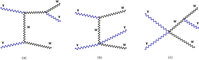
Figure 2: Representative Feynman diagrams for $\gamma\gamma\rightarrow W^{+}W^{-}\gamma$ production at tree level.

In this work, we use the MadGraph5_aMC@NLO package [64, 65] in order to generate the SM processes and signal processes with aTGCs and aQGCs. In order to simulate the photon emission from incoming protons for the processes with photon-photon interaction, the photon PDF based on the equivalent photon approximation for low-virtuality photons has been implemented in MadGraph5_aMC@NLO [57]. To calculate the total cross section, W-boson mass $m_{W}$= 80.37 GeV and $G_{F}=1.16639\times 10^{-5}{\mathrm{GeV}^{-2}}$ is considered. To calculate the cross section and generate the events of WW$\gamma$ process, including aTGCs and aQGCs, we use the FeynRules package [66] to convert the effective Lagrangian to the UFO model [67] which can be linked to the MadGraph5_aMC@NLO. MadGraph5_aMC@NLO is also used to generate several photon-photon or parton-parton initiated background processes. To perform parton showering and hadronization, all the generated samples are passed through Pythia 8 [68]. In this analysis, we also consider the fast simulation of LHC-like detectors to consider the effects of detector response on the final reconstructed objects using the Delphes 3.4.1 package [69].

5 Analysis Design

In this section, we describe the strategy for analysis including the object selection cuts, event selections and discuss the contribution of each source of background. Depending on the flavor of leptons decayed from W boson, we divide our signal region into the same flavor leptonic (SF) channel consists of $e^{+}e^{-},\mu^{+}\mu^{-}$ events and different flavor (DF) channel $e^{+}\mu^{-},e^{-}\mu^{+}$, because the SF channel suffers from a large contribution of $l^{+}l^{-}\gamma$ background process while DF does not.

5.1 Selection cuts

In order to select the $WW\gamma$ signal events including the SM or anomalous coupling contributions, we apply three categories of selection cuts. The first set of cuts includes the central detector requirements which are applied in order to select the objects needed to construct the signal final state events and suppress the backgrounds, optimally. The second set of cuts is applied to the tagged protons in order to adopt the acceptance of the FDs. The third type of cuts is beneficial form the kinematic correlation of central produced state and detected protons in the FDs to reject non-exclusive backgrounds as well as exclusive backgrounds with the different expected proton’s kinematics according to the signal. For the first category of cuts (type I), we require to have two opposite sign well-isolated leptons, both of them required to have $p_{T,l}>10$ GeV but at least one of them must pass $p_{T,l}>20$ GeV and both are required to be in $|\eta_{l}|<$2.5. It should be pointed out that required $p_{T,l}$ thresholds are totally in agreement with the current thresholds of double lepton triggers which are used in the current experiments such as CMS. Therefore one expects the high trigger efficiency considering these cut values. In addition, we veto events containing any extra loose lepton with $p_{T,l}>10$ GeV and $|\eta_{l}|<$ 2.5 in order to suppress the contribution from $WZ\gamma$, $ZZ\gamma$ background processes. We also demand to have exactly one isolated photon with $p_{T,\gamma}>20$ GeV and $|\eta_{\gamma}|<$ 2.5. To suppress the backgrounds without W boson, we require the missing transverse energy, $\not{E}>30{{\rm\ GeV}}$. In order to suppress the contribution of events with a photon radiating from W and Z decay product as well as preventing the drop of reconstruction efficiency due to the close-by lepton from photon, we require to have $\Delta R_{\gamma,l}=\sqrt{\Delta\phi^{2}+\Delta\eta^{2}}>$ 0.5. The last criteria to suppress the backgrounds containing jets such as inclusive $t\bar{t}\gamma$, is to veto events containing more than one jets with $p_{T,j}>$40 GeV and $|\eta_{j}|<$5.0. The reason to apply veto cut on the number of jets $N_{j}>2$ is that the probability to reconstruct a jet from pile-up is not negligible in high pile-up conditions, even for purely leptonic signal events. Therefore, to maintain the optimum amount of signal versus high rejection of backgrounds, we loosen the number of jets in the veto condition. In the second type of cuts (type II) we require to have at least one proton in each side of interaction point to be within the FD acceptance. The acceptance of the detector is usually expressed in terms of the fractional energy loss of each proton. In this analysis, we consider two scenarios for FD acceptance corresponding to $0.0015<\xi<0.2$ and $0.0015<\xi<0.5$. However, in order to suppress the different sources of backgrounds, we require $\xi$ to be greater than 0.008. Figure 3 (left) indicates the distribution of fractional energy loss of both protons reaching the forward detectors. One could see from Figure 3 (left) that applying a lower cut on the $\xi$ will reduce the contribution of photon initiated backgrounds as well as pile-up backgrounds, effectively. Furthermore, we exploit from the high correlation of primary vertex (PV) displacement in the $z$-direction and arrival time of both tagged protons to the timing FDs in the CEP processes, to put down the inclusive background contribution, effectively.

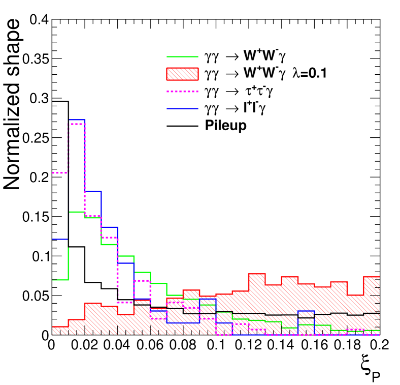
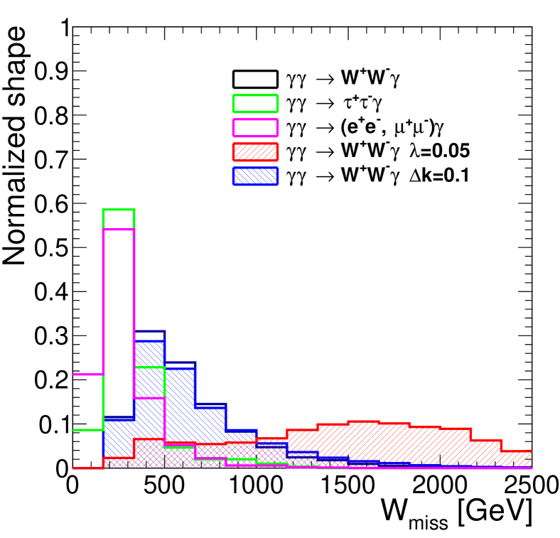
Figure 3: Distribution of fractional energy loss of protons reaching the FDs (left) and protons missing mass (right) for SM $\mathrm{p}\mathrm{p}\rightarrow\mathrm{p}W^{+}W^{-}\gamma\mathrm{p}$, $\mathrm{p}\mathrm{p}\rightarrow\mathrm{p}l^{+}l^{-}\gamma\mathrm{p}$ and two $\mathrm{p}\mathrm{p}\rightarrow\mathrm{p}W^{+}W^{-}\gamma\mathrm{p}$ samples including aTGCs correspond to $\lambda_{\gamma}=0.05$ and $\Delta\kappa=0.05$.

For the third type of requirements (type III), we restrict the protons missing mass $W_{\text{miss}}$ to be larger than 200 GeV. As indicated in Figure 3 (right) protons missing mass for the CEP $W^{+}W^{-}\gamma$ starts from 200 GeV which is approximate energy for the production of two on-shell W bosons. While for the less heavy state such as the CEP $l^{+}l^{-}\gamma$, the threshold is smaller. Therefore, having this cut effectively reduces the contribution of photon-photon initiated $l^{+}l^{-}\gamma$ background. In addition to that, one can use the conservation of momentum in the $z$-direction in order to obtain the missing longitudinal momentum of the central system. Thus, the central mass can be reconstructed partially and could be used to reject both the CEP and inclusive backgrounds when it is compared to the protons missing mass. This cut will be explained and discussed in detail in Section 5.3.

5.2 Pile-up Implementation

Pile-up is referred to the multiple soft proton-proton interactions in each bunch crossing of the LHC which is happening along with the hard process coming from the PV. The average number of pile-up interactions per bunch crossing $<N_{PU}>$ is depended on the condition of the machine that collides the protons to each other, such as the energy of protons, the number of protons in each bunch and etc. The mean value of pile-up at the LHC varies between 20-50 from Run I to II and the expectation for high luminosity LHC is between the 140-200. The overall effect of pile-up interaction is the production of soft hadrons that propagate to all layers of detectors and biases the measured quantities and degrade the resolution of the reconstructed final state particles of hard processes. In order to estimate the effects of the pile-up interactions, we simulate the minimum bias events using the Pythia 8. Then the superposition of generated minimum bias events and the PV of hard processes is performed using the Delphes 3.4.1. In order to implement pile-up interactions in each event we take similar parameters that considered for modeling pile-up in the CMS detector at the LHC. In this analysis the simulation of all the signal and background samples are performed, considering the average number of pile-up as $<N_{PU}>$= 30. In this analysis, the variables which are affected by the pile-up are isolation of leptons, photons as well as missing energy. Therefore, to alleviate the effects of pile-up, we subtract the contribution of soft charged particles originated from the vertices which are far enough from the primary vertex. Furthermore, to remove the contribution of neutral pile-up the FastJet area method is used [70]. This method considers the homogeneous energy density imposed by neutral pile-up particles and the area where the isolation of leptons and photons are effected to subtract the neutral contribution of the pile-up. In addition to the above effects, the presence of the pile-up in the exclusive searches is very important as they can produce protons that may lay in the acceptance of FDs. We will discuss the effects of these detected protons in the next section.

5.3 Inclusive backgrounds with Pile-up protons

One of the main sources of background processes that can contribute to our signal regions is non-exclusive backgrounds. The main processes which can produce a similar signature as our signal in the central detector are $t\bar{t}\gamma,l^{+}l^{-}\gamma,W^{+}W^{-}\gamma,W^{+}Z\gamma,ZZ\gamma$. The cross sections of these processes are several orders of magnitudes larger than the signal. They may pass the type I selection requirements. However, they can contribute to our signal region only if they pass also the type II and III selection cuts. This can happen if the event of such inclusive processes coincides with protons in the acceptance of FDs produced by pile-up interactions. The main proton-proton processes that may produce protons in the FDs are elastic and single diffractive processes. Other interactions such as double diffractive and non-diffractive processes have fewer contributions as these interaction does not produce intact protons directly and the trapped protons from these processes can result from the dissociation of incoming protons. In addition, the elastic interactions suppress heavily due to the lower cut on the proton acceptance region $\xi>$ 0.008, introduced in the previous section, as the outgoing protons are expected to have very small $\xi$. Therefore, the main process that can produce two detectable protons on each side of FDs is from multiple single diffractive processes that occur at each proton bunch crossing. The appearance of protons in the FDs due to pile-up is independent of inclusive processes and vary only by changing the average number of pile-up. Therefore, the fraction of events that have at least one proton in the acceptance region of each side of FDs, as well as events that satisfy the timing requirement, can be calculated as an independent factor from the specific inclusive processes. Then to obtain the backgrounds yield after applying the Type II selection cuts, one can multiply the number of inclusive events that remain after central selection cuts by these calculated efficiencies. We will calculate and report the type II selection cut efficiencies for different pile-up scenarios that can be used for any study including this type of background.

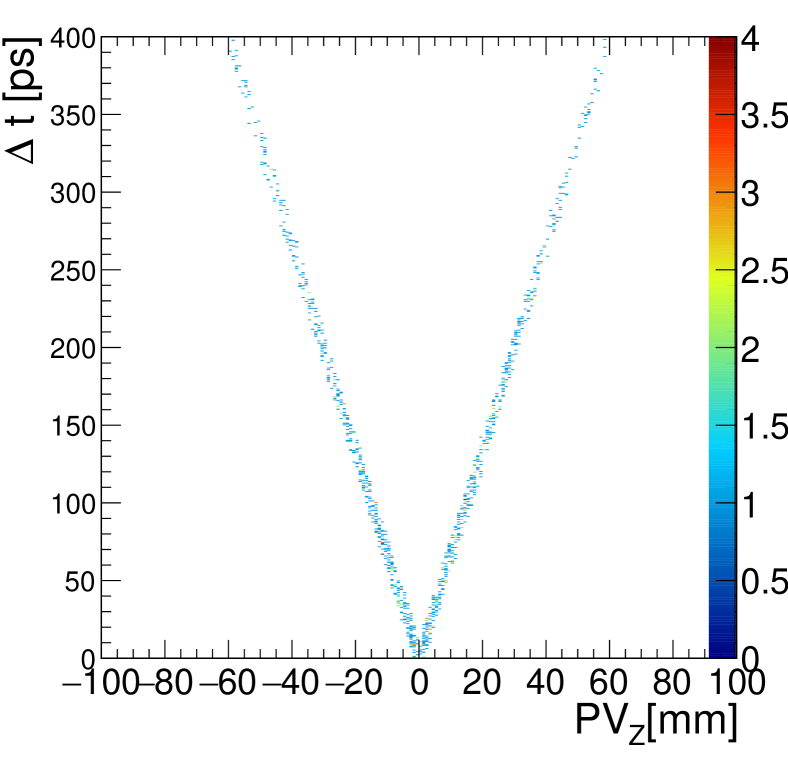
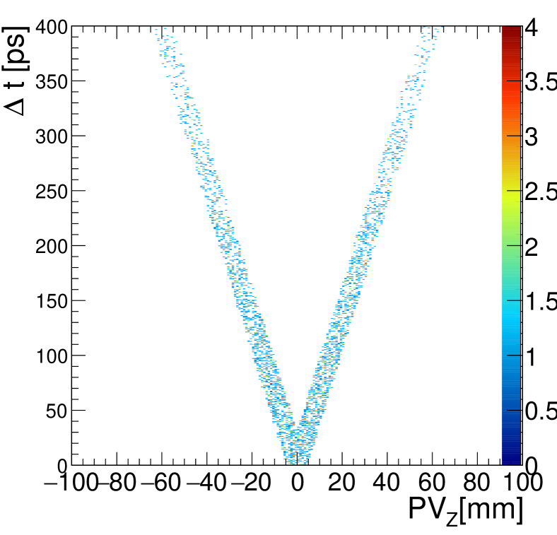
Figure 4: Absolute time of flight difference of two protons detected in the timing FDs versus PV position in $z$-direction, considering 10 ps(left) and 30 ps(right) resolutions. This correlation is calculated for the SM process $\mathrm{p}\mathrm{p}\rightarrow\mathrm{p}W^{+}W^{-}\gamma\mathrm{p}$.

The type II selection cuts described in Section 5.1 except for the timing requirement which will be discussed here.

In the CEP processes primary vertex position in the longitudinal direction is proportional to the difference between the arrival time of two protons to the FDs as $z_{\text{PV}}\propto\frac{(t_{1}-t_{2})}{2}$, while for inclusive processes superposed by the pile-up protons are not. Therefore, depending on the timing resolution of time of flight detectors, it could be used to reject the inclusive backgrounds several orders of magnitudes. The benchmark resolution considered for timing FDs is between the 10-30 ps [71, 46] corresponds to the uncertainties of $\sigma_{\text{PV}_{z}}=$ 2.1 and 6.3 mm on the PV position, respectively. Figure 4 shows the correlation between the displacement of the primary vertex in $z$-direction and the absolute difference between the arrival time of two tagged protons in the FDs for the SM $W^{+}W^{-}\gamma$, CEP process assuming the 10 ps (left) and 30 ps (right) resolutions for timing detectors. inclusive background processes will pass the timing cut if the distance between vertex position obtained from pile-up protons and the PV position is closer than 2.1 (6.3) mm for considered resolutions of 10 (30) ps, respectively. These distance values can be obtained simply from timing resolutions of FDs. In order to apply this requirement, one needs to select one pair of protons out of different possible combinations. Because the number of pile-up protons that reach the timing FDs can be exceeded from two. Figure 5 indicates the multiplicity of protons passing the acceptance cuts.

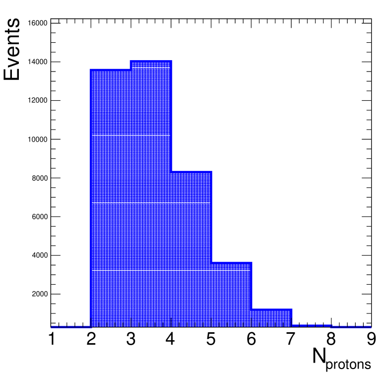
Figure 5: Multiplicity of pile-up protons passing the $0.008<\xi<0.2$ FDs acceptance. The average number of pile-up is $<N_{PU}>$=30 per event. The number of generated pile-up events are 100k.

Therefore, we require to select a pair of protons which is placed in the closest distance w.r.t to the PV by defining the $\delta r=\sqrt{(Z_{\text{PV}}-Z_{\mathrm{p}1})^{2}+(Z_{\text{PV}}-Z_{\mathrm{p}2})^{2}}$ where, the $Z_{\mathrm{p}1,\mathrm{p}2}$ are vertex position of each tagged protons, and $Z_{\text{PV}}$ is the vertex position of PV in the $z$-direction. Thus, a pair of protons with the smallest value of $\delta r$ in each event is selected. Figure 6 shows the distribution of PV position of $W^{+}W^{-}\gamma$ inclusive process versus absolute difference arrival time of two selected pile-up protons.

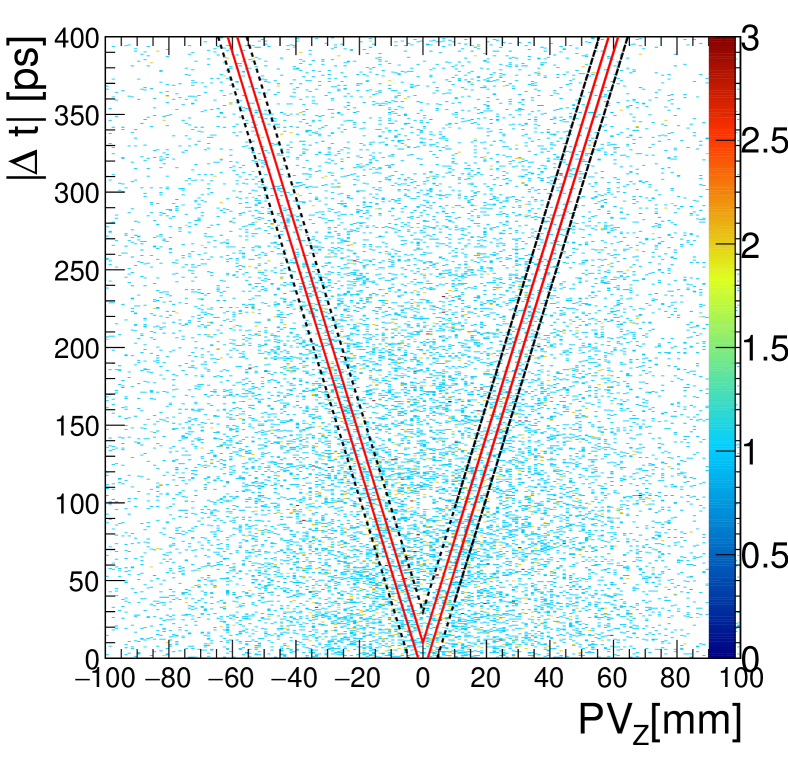
Figure 6: Distribution of absolute time difference of superimposed pile-up protons tagged in the FDs versus displacement of PV in the $z$-direction for inclusive $W^{+}W^{-}\gamma$ process. The protons are restricted to pass $0.008<\xi<0.2$ requirement. The average number of pile-up per each bunch crossing is $<N_{PU}>$=30. The events between red (black dashed) lines will pass the timing requirement due to coincidence of pile-up protons with their PV position considering 10(30) ps resolutions.

The area enclosed between the red (black dashed) lines represents accepted inclusive events that the time difference of the arrival of their tagged protons falls within the uncertainty range of the PV position imposed by the timing detector resolutions of 10(30) ps. Table 1 shows the calculated fraction of events remained after applying the acceptance cut as well as the time of flight (TOF) cuts for the average number of pile-up from $<N_{PU}>$=10-140, assuming two scenarios for protons acceptance. It is clear from Table 1 that the probability of pile-up protons tagged in the FDs increases with rising the average number of pile-up $<N_{PU}>$. Therefore, it is necessary to pay careful attention to the inclusive background processes along with the pile-up protons in the high pile-up condition to estimate the realistic background contribution.

The last category of selection cuts which we call it type III, depends on both the central state and tagged proton kinematics. The first requirement is a lower cut on the $W_{\text{miss}}$ which is explained in the section 5.1. In addition to that, in the CEP processes, one can reconstruct the mass of central system from the fractional energy loss of both tagged protons $W_{\text{miss}}$, whereas it is not true if the protons come from pile-up interaction, explained earlier in this section.

Double tagging efficiency
	$<N_{PU}>$	10	30	50	100	140
Type II	$0.0015<\xi<0.2$	0.06	0.31	0.56	0.87	0.95
	$0.0015<\xi<0.5$	0.30	0.81	0.95	0.99	1.00
	$\xi>0.008$	0.03	0.19	0.38	0.73	0.86
		0.26	0.76	0.93	0.99	1.00
	TOF	0.001	0.008	0.016	0.036	0.048
		0.010	0.04	0.06	0.011	0.157

Table 1: The fraction of remained events assuming the FDs acceptance, lower cut on the $\xi_{1,2}$, and TOF requirement for different average numbers of pile-up are reported. At least one proton on each side of interaction point is required. The obtained fraction of events at each level includes all other previous cuts. The efficiency of double proton tagging is increased by rising the number of pile-up.

Therefore, in the case of full reconstruction of the central system, there will be a direct correlation between $M_{X}$ with $X=l_{1}l_{2}\gamma(\nu_{1}+\nu_{2})_{\text{rec}}$ and $W_{\text{miss}}$ which results to significant rejection of backgrounds. On the other hand, there is a source of ambiguity in the di-leptonic channel of the central system of our interest CEP $W^{+}W^{-}\gamma$ (either the SM or including the anomalous couplings) process, due to the presence of two neutrinos. Regarding the neutrinos, the only known information from central detector is the sum of missing energy in $x$ and $y$ directions, while the presence of FDs allows us to obtain the total missing momentum in the $z$-direction via conservation of momentum in the longitudinal direction

$$p_{z}(l_{1})+p_{z}(l_{2})+p_{z}(\gamma)+p_{z}(\nu_{1}+\nu_{2})=p_{z}(\mathrm{p}_{1})+p_{z}(\mathrm{p}_{2}).$$ (14)

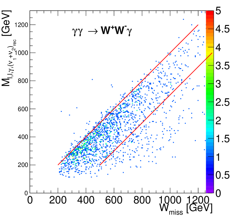
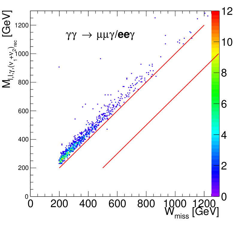
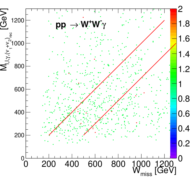
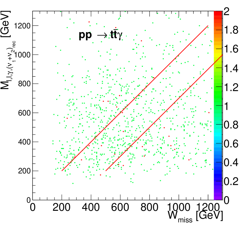
Figure 7: Two-dimensional distributions of reconstructed invariant mass of central system versus protons missing mass. The constructed invariant mass is obtained by summation of four-momentum for two leptons, photon, and four-momentum sum of two neutrinos. The left-top and right-top plots show these two-dimensional distributions for $\gamma\gamma\rightarrow W^{+}W^{-}\gamma$ and $\gamma\gamma\rightarrow l^{+}l^{-}\gamma$ processes, respectively. The left-bottom and right-bottom plots belong to the inclusive $W^{+}W^{-}\gamma$ and $t\bar{t}\gamma$ processes superimposed by pile-up protons. The events surrounded between two red lines will be kept by the Type III cut.

Then, one could obtain the invariant mass of the central system by summing over four-momentum of leptons, photons, and  total missing energy as $M_{l_{1}l_{2}\gamma(\nu_{1}+\nu_{2})_{\text{rec}}}=(p({l_{1}})+p({l_{2}})+p(\gamma)+p{(\nu_{1}+\nu_{2})_{\text{rec}}})^{2}$. However, we are not fully aware of four-momentum components of each neutrino that lead to expansion of correlation between the reconstructed invariant mass of the central system and $W_{\text{miss}}$. Figure 7 top-left indicates this behavior for the CEP $W^{+}W^{-}\gamma$ process. Having this characteristic, we require the 0 $<W_{\text{miss}}-M_{{l_{1}l_{2}\gamma(\nu_{1}+\nu_{2})}_{\text{rec}}}<$ 300 which is the region depicted between the red lines. Fortunately, even looser correlation is sufficient to reject inclusive $W^{+}W^{-}\gamma$ ($t\bar{t}\gamma$) backgrounds showing in the bottom left (right), respectively. Table 2 shows the number of inclusive backgrounds after applying each set of selection cuts. The final yields are represented for 300 $\,{\rm fb}^{-1}$ IL.

($\mathcal{L}=300\,{\rm fb}^{-1},\sqrt{s}=13{\rm\ TeV}$) $\mathrm{p}\mathrm{p}\rightarrow\tau\bar{\tau}\gamma$ $\mathrm{p}\mathrm{p}\rightarrow t\bar{t}\gamma$ $\mathrm{p}\mathrm{p}\rightarrow W^{+}W^{-}\gamma$ $\mathrm{p}\mathrm{p}\rightarrow ZZ\gamma$ $\mathrm{p}\mathrm{p}\rightarrow W^{\pm}Z\gamma$ $\mathrm{p}\mathrm{p}\rightarrow l\bar{l}\gamma$ $e\mu(ee+\mu\mu)$ $e\mu(ee+\mu\mu)$ $e\mu(ee+\mu\mu)$ $e\mu(ee+\mu\mu)$ $e\mu(ee+\mu\mu)$ $e\mu(ee+\mu\mu)$ Type I $p_{T,l_{1}}>20{{\rm\ GeV}},p_{T,l_{2}}>10{{\rm\ GeV}}$ 8519 (8411) 6106(6089) 560 (588) 0.07 (4) 23 (114) 949 (418763) $|\eta_{l_{1},l_{2}}|<2.5$, $iso<0.15$ $\not{E}>30{{\rm\ GeV}}$ 4106 (4191) 5447(5409) 447 (469) 0.05 (2.2) 18 (92) 501 (171067) $p_{T,\gamma}>20{{\rm\ GeV}}$,$|\eta_{\gamma}|<2.5$, $iso<0.15$ 1141 (1124) 2709(2516) 204 (210) 0.02 (1) 8 (41) 43 (60093) $\Delta R_{\gamma,l_{1}}>0.5$, $\Delta R_{\gamma,l_{2}}>0.5$ Veto $N_{j}>2$, $p_{T,j}>40{{\rm\ GeV}}$ 1124(1119) 1101(1034) 201(205) 0.02(0.82) 7.77(39) 33(59649) $|M_{l_{1}l_{2}}-m_{Z}|>10{\rm\ GeV}$ 1090 (1107) 282 (266) 609 (622) 0.015(0.07) 6.9 (8.8) 5(4446) Type II $0.008<\xi<0.2$ 182(187) 207(197) 38(39) 0.005(0.01) 1.2(1.8) 0(1035) $0.008<\xi<0.5$ 858(772) 219(202) 137(140) 0.01 (0.06) 5.3 (7) 19(3396) TOF 0 (0) 5.4(3.4) 0.88(0.75) 0(0) 0.03 (0.006) 0(19) 23(23) 17(24) 3.3 (4) 0(0.0009) 0.14(0.2) 0 (100) Type III $W_{\text{miss}}>200{\rm\ GeV}$ 0(0) 5.4(2.75) 0.76 (0.75) 0 (0) 0.03(0.006) 0(19) 23(23) 17 (24) 3.3(4) 0(0.0009) 0.14(0.2) 0 (100) 0 $<W_{\text{miss}}-M_{l_{1}l_{2}\gamma(\nu_{1}+\nu_{2})_{\text{rec}}}<$ 300 0 (0) 0(0) 0.13 (0.06) 0 (0) 0(0) 0(0) 0 (0) 1.36(0) 0.126 (0.126) 0(0.0009) 0.006(0.006) 0(0)

Table 2: The remaining yields of the SM inclusive background processes coincide with pile-up protons after each type of selection cuts for $300\,{\rm fb}^{-1}$ IL are presented. The mean number of modeled pile-up set to 30.

($\mathcal{L}=300\,{\rm fb}^{-1},\sqrt{s}=13{\rm\ TeV}$) $\gamma\gamma\rightarrow W^{+}W^{-}\gamma$ $\gamma\gamma\rightarrow\tau\bar{\tau}\gamma$ $\gamma\gamma\rightarrow l^{+}l^{-}\gamma$ $e\mu(ee+\mu\mu)$ $e\mu(ee+\mu\mu)$ $e\mu(ee+\mu\mu)$ Type I $p_{T,l_{1}}>20{{\rm\ GeV}},p_{T,l_{2}}>10{{\rm\ GeV}}$ 3.3 (3.4) 2.1 (2.2) 0.7 (464) $|\eta_{l_{1},l_{2}}|<2.5$, $iso<0.15$ $\not{E}>30{{\rm\ GeV}}$ 2.9 (2.9) 1.3 (1.4) 0.34 (188) $p_{T,\gamma}>20{{\rm\ GeV}}$,$|\eta_{\gamma}|<2.5$,$iso<0.15$ 1.5 (1.5) 0.5 (0.5) 0.02 (60) $\Delta R_{\gamma,l_{1}}>0.5$, $\Delta R_{\gamma,l_{2}}>0.5$ Veto $N_{j}>2$, $p_{T,j}>40{{\rm\ GeV}}$ 1.5 (1.5) 0.5 (0.4) 0.03 (60) $|M_{l_{1}l_{2}}-m_{Z}|>10{\rm\ GeV}$ 1.4 (1.4) 0.46 (0.4) 0.01 (52) Type II $0.008<\xi<0.2$,TOF 1.2 (1.2) 0.2 (0.3) 0 (17) $0.008<\xi<0.5$, TOF 1.28 (1.26) 0.22 (0.27) 0 (17) Type III $W_{\text{miss}}>200{\rm\ GeV}$ 1.2 (1.2) 0.18 (0.2) 0 (12) 1.28 (1.26) 0.18 (0.23) 0 (12) 0 $<W_{\text{miss}}-M_{l_{1}l_{2}\gamma(\nu_{1}+\nu_{2})_{\text{rec}}}<$ 300 0.94 (0.94) 0.15 (0.2) 0 (0.066) 0.98 (0.99) 0.15 (0.2) 0 (0.067)

Table 3: The remaining yields of the SM $\gamma\gamma\rightarrow W^{+}W^{-}\gamma$, $\gamma\gamma\rightarrow\tau^{+}\tau^{-}\gamma$, and $\gamma\gamma\rightarrow e^{+}e^{-}\gamma/\mu^{+}\mu^{-}\gamma$ after each type of selection cuts for $300\,{\rm fb}^{-1}$ IL are presented.

5.4 $\gamma\gamma$-initiated background processes

One of the main sources of backgrounds to our exclusive $W^{+}W^{-}\gamma$ process is from the processes with the same mechanism of photon-photon interactions at the LHC. Among them, the dominant background is the production of $\gamma\gamma\rightarrow l^{+}l^{-}\gamma$ which the leptons can be either electron, muon or tau (if tau decays leptonically). The $e^{-}e^{+}\gamma,~{}\mu^{-}\mu^{+}\gamma$ channels are dominant in the SF signal region while the $\tau^{-}\tau^{+}\gamma$ can contribute equally in both SF and DF signal regions. We applied the three types of selection cuts described in the previous sections. Table 3 shows the number of events for the SM $W^{+}W^{-}\gamma$ exclusive process and their photon-photon initiated backgrounds after each set of selection cuts and assuming 300 $\,{\rm fb}^{-1}$ expected IL. It is interesting to mention that the correlation between the reconstructed mass of the central system and protons missing mass for $l^{+}l^{-}\gamma$ background which is depicted in Figure 7 (top-right) is completely different from the SM $W^{+}W^{-}\gamma$ mass correlation. Table 3 shows a large amount of this background remains after type I and II, but reduced to the zero level considering this cut.

5.5 Double pomeron exchange processes

In addition to central exclusive production via $\gamma\gamma$ interaction, $W^{+}W^{-}\gamma$ and $l^{+}l^{-}\gamma$ processes can occur through the double pomeron exchange (DPE). The pomeron is believed to carry the quantum numbers of vacuum, thus they will be colorless states in QCD language. It is also proposed that pomeron has partonic structure such as hadrons [72, 73]. Therefore, hard diffractive processes can be described in terms of single and double pomeron exchange between two protons based on the Ingelman-Schlein approach [74] that has been searched in the different experiments ever since [75, 76, 77]. In this model, cross section of the DPE can be factorized into the diffractive parton distribution functions and matrix element of hard interaction between the pomeron constituents that considered to be gluonic. Currently, several MC generators such as Forward Physics Monte Carlo (FPMC) generator [78] can calculate the cross section and generate events of the DPE processes such as dilepton, di-boson, and di-jet productions. Since our favorite $\text{DPE}\rightarrow W^{+}W^{-}\gamma$ and $\text{DPE}\rightarrow l^{+}l^{-}\gamma$ processes are not yet implemented in any generators, we inevitably have considered some assumptions in order to extract their contribution into the SM signal and background processes. According to [74] the cross section of $\text{DPE}\rightarrow W^{+}W^{-}\gamma$ and $\text{DPE}\rightarrow l^{+}l^{-}\gamma$ can be factorized into the scattering amplitude of emerging partons from each pomeron and already known diffractive PDF. On the other hand the cross section of inclusive $W^{+}W^{-}\gamma$ and $l^{+}l^{-}\gamma$ from proton-proton collision also can be factorized into the matrix element of partonic interaction by the PDF of protons. Therefore, one can assume the equality of cross section ratios of inclusive and DPE as following

$$\frac{\sigma_{\mathrm{p}\mathrm{p}\rightarrow W^{+}W^{-}/l^{+}l^{-}}}{\sigma_{\mathrm{p}\mathrm{p}\rightarrow W^{+}W^{-}\gamma/l^{+}l^{-}\gamma}}=\frac{\sigma_{\text{DPE}\rightarrow W^{+}W^{-}/l^{+}l^{-}}}{\sigma_{\text{DPE}\rightarrow W^{+}W^{-}\gamma/l^{+}l^{-}\gamma}}.$$ (15)

We calculated the ratios $\frac{\sigma_{\mathrm{p}\mathrm{p}\rightarrow W^{+}W^{-}/l^{+}l^{-}}}{\sigma_{\mathrm{p}\mathrm{p}\rightarrow W^{+}W^{-}\gamma/l^{+}l^{-}\gamma}}$ by MadGraph5_aMC@NLO at tree level for $W^{+}W^{-}\gamma$ and $l^{+}l^{-}\gamma$ processes resulting to values of 243.3 and 92.5, respectively. Due to the existence of a photon in the matrix element of the denominator, one would expect the ratio to be around $1/\alpha\simeq$ 100 where the $\alpha$ is Fine-structure constant. The di-lepton production to the di-lepton plus photon cross section ratio seems to agree with this expectation, but the di-boson ratio is more than twice as high the expected ratio. The reason is behind the contributed Feynman diagrams with triple and quartic gauge boson couplings which have destructive interference and lead to lower cross section ratio w.r.t di-leptonic ratio. We also calculate the cross sections of DPE$\rightarrow W^{+}W^{-}$ and DPE$\rightarrow l^{+}l^{-}$ using FPMC generator at 13 TeV and obtain the corresponding values of 1.35 and 701.4 pb for these two processes, respectively. Having the left-hand-side of equation 15 also the numerator of right-hand-side we obtain 5.5 fb and 7.58 pb for the cross section of DPE$\rightarrow W^{+}W^{-}\gamma$ and DPE$\rightarrow l^{+}l^{-}\gamma$, respectively. Furthermore, the obtained cross sections have to be multiplied by a gap survival probability for QCD diffractive and central exclusive productions which is 0.03[79]. This factor accounts for the probability that the gaps are surviving from the presence of extra particles in the interaction. This rapidity gap can be washed out mainly by soft inelastic interaction that produces some secondary particles or re-scattering of leading hadron or hard QCD bremsstrahlung. In order to estimate the contribution of these two DPE processes in our signal regions we assumed that the kinematics of their final state are similar to the $\gamma\gamma\rightarrow l^{+}l^{-}\gamma$ and $\gamma\gamma\rightarrow W^{+}W^{-}\gamma$. Therefore, we obtain the efficiency of type I and type II selection cuts from photon initiated processes and apply these efficiencies as a new factor to the similar DPE processes. The summary of factors which are applied to the DPE processes and their final contributions in the two signal regions using $300\,{\rm fb}^{-1}$ IL is shown in Table 4.

6 SM $\gamma\gamma\rightarrow W^{+}W^{-}\gamma$ measurement

Considering the small predicted cross section of central exclusive $W^{+}W^{-}\gamma$ process, the measurements of this process needs a high amount of data. On the other hand, the advantage of having timing and tracking FDs allows us to measure this process in the high pile-up run conditions of the LHC, also bring the backgrounds of this process in very small amount as shown in detail in the previous sections. We consider the fully leptonic decay of W bosons in the SF and DF channels. In order to calculate the potential discovery of this process, we use Profile Likelihood formalism. The median significance assuming the signal hypothesis $\mu$=1 can be obtained by

$$\text{med}[Z_{0}|1]=\sqrt{2((s+b)ln(1+s/b)-s)},$$ (16)

where s and b are the number of signal and backgrounds [80]. Figure 8 illustrates the potential observation of this process considering only di-leptonic channel as a function of IL.

Backgrounds
Process	DPE$\rightarrow W^{+}W^{-}\gamma$	DPE$\rightarrow l^{+}l^{-}\gamma$
Total cross section [fb]	5.5	7583
Gap survival rapidity [fb]	0.165	227.49
Type I selection cut eff [fb]	0.002	0.36
Type II selection cut eff [fb]	4e-6 (1e-4)	0e-5 (0e-5)
Type III selection cut eff [fb]	0e-6 (0e-4)	0e-5 (0e-5)
Final yield for 300 $\,{\rm fb}^{-1}~{}(ee,\mu\mu,e\mu))$	0e-6 (0e-4)	0e-5 (0e-5)

Table 4: The sequence of different type of cuts on the cross sections of DPE$\rightarrow W^{+}W^{-}\gamma$ and DPE$\rightarrow l^{+}l^{-}\gamma$ processes in two signal regions are presented. The last row represents the final yields for 300 $\,{\rm fb}^{-1}$ IL.

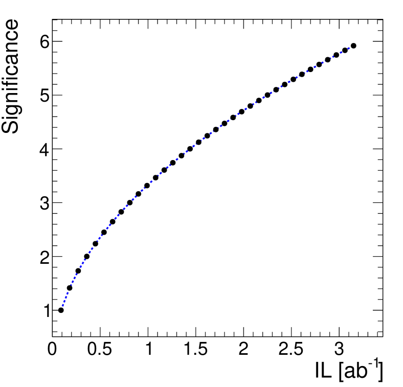
Figure 8: Expected significance as a function of IL for the SM central exclusive production of $W^{+}W^{-}\gamma$ process using only di-leptonic channel.

The amount of data for having a strong evidence of this process with 3$\sigma$ significance is about the 0.8 $\,{\rm ab}^{-1}$ while for full observation of this process with 5$\sigma$ significance one expected 2.1 $\,{\rm ab}^{-1}$ IL. The observation of this process is not the most interesting aspect of this study but rather the power of this process to constrain anomalous couplings due to very low amount of backgrounds which is going to be discussed in next two sections. It should be mentioned that estimated amount of data needed to observe this process, given in Figure 8, is obtained from the extrapolation of the present study based on $<N_{PU}>=30$.

7 Sensitivity to anomalous gauge boson couplings

In this section, we discuss the potential of $W^{+}W^{-}\gamma$ CEP to probe aTGCs and aQGCs at the LHC using forward detectors. In order to reach the highest sensitivity, one needs to study these new couplings in the signal dominated region. Therefore, we need to modify the type III of introduced cuts in the previous sections. The first modification is to restrict the lower cut on the protons missing mass to more than 900 GeV, as the contribution of anomalous couplings is enhanced at high missing mass values while the backgrounds are effectively suppressed. Figure 3 right shows the distribution of protons missing mass for two scenarios of anomalous couplings, SM $W^{+}W^{-}\gamma$ CEP as the irreducible background, and some other photon initiated backgrounds. In addition to this change, we introduce a new cut on the invariant mass of visible central state ${\it i.e.}$ lepton pair and photon. We restrict the invariant mass of lepton pair and photon to be higher than 200 and 500 GeV for the two considered scenarios of acceptance. Even though this cut is highly correlated with the previous cuts for photon initiated backgrounds, it is fully independent for inclusive backgrounds with pile-up protons. Therefore, this cut effectively suppresses inclusive backgrounds while it is safe for keeping the signal contribution. Figure 9 illustrates the invariant mass of lepton pair and photon for some of photon initiated and inclusive backgrounds as well as two considered anomalous signals. We also require the difference between the missing mass of protons and reconstructed mass state only to be greater than zero as we observed the correlation between these two masses behave differently from what indicated in Figure 7 top-left when one includes the anomalous couplings. Thus, to avoid the drop in signal efficiency we loosen this criterion.

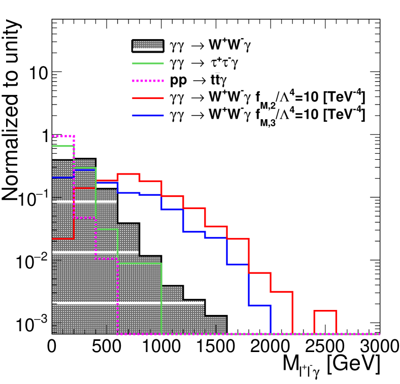
Figure 9: The invariant mass distribution of $l_{1}l_{2}\gamma$, measured in the central detector. The SM backgrounds are indicated in shaded gray, solid green and dashed purple histograms. The red and blue histograms show the two samples of dimension-8 coupling $f_{M,2}/\Lambda^{4}=f_{M,3}/\Lambda^{4}=10{\rm\ TeV}^{-4}$.

($\mathcal{L}=300\,{\rm fb}^{-1},\sqrt{s}=13{\rm\ TeV}$)	Backgrounds	$\lambda=0.05$	$f_{M,1}/\Lambda^{4}=10{\rm\ TeV}^{-4}$	$f_{M,3}/\Lambda^{4}=10{\rm\ TeV}^{-4}$
	$e\mu+ee+\mu\mu$	$e\mu+ee+\mu\mu$	$e\mu+ee+\mu\mu$	$e\mu+ee+\mu\mu$
Type I	6745.9	116	3.5	64
TOF,$0.008<\xi<0.2(0.5)$	38.8 (71.3)	7(85)	1.8 (2.9)	3 (43)
$W_{\text{miss}}>900,M_{l^{+}l^{-}\gamma}>200(500){\rm\ GeV},$	0.3 (0.9)	7(79)	0.3 (1.1)	2 (38)
$W_{\text{miss}}-M_{l_{1}l_{2}\gamma(\nu_{1}+\nu_{2})_{\text{rec}}}>0$

Table 5: The yield of the SM backgrounds and few signal samples after applying the Type I cut, modified Type II, and Type III cuts for 300 f$\text{b}^{-1}$ IL. The considered signal samples are $\lambda=0.05$ and $f_{M,1}/\Lambda^{4}=f_{M,3}/\Lambda^{4}=10{\rm\ TeV}^{-4}$.

Table 5 shows the effect of each type of selection cuts on the total SM backgrounds including the photon initiated, DPE, and inclusive backgrounds and few cases of aQGCs and aTGCs.

An important subject in studying the anomalous gauge boson couplings is to check for the preservation of unitarity. It is well understood that the non-zero value of new EFT operators could result in the rapid increase of scattering amplitude w.r.t the energy which could violate the unitarity in the sufficient high center-of-mass energy of colliding partons. In this analysis, the presence of dimension-6 and -8 effective operators could potentially cause this violation. However, considering the FDs acceptance e.g 0.008$<\xi<$ 0.2 prevents the center-of-mass energy of two colliding photons from exceeding 2.5 GeV which is shown to be approximately safe [81]. For other cases in which the acceptance cut is not sufficient to exclude the regions which unitarity is not preserved one usually uses the form factors (FFs). These FFs essentially are energy dependent cutoff of a complete model at the scale of $\Lambda$ which is integrated out as the higher-order EFT operators. A dipole FF or a sharp cutoff on the EFT operators at a fixed energy scale is usually considered to control the unitarity. In the EFT description which is a model-independent approach, there is no preferred method or functionality for FFs. Therefore, various forms of FFs are considered in the literature. In this analysis, to compare our results in a FF independent way with several experimental measurements [8, 83, 82, 48, 84], we also do not apply any unitarity dipole form factor or cutoff.

7.1 Statistical method

In this section, we discuss the potential of this channel to constrain aTGCs and aQGCs assuming one and two-dimensional scan of effective couplings. We use the signal region defined in Table 5 in order to count the contribution of signal and SM backgrounds in both SF and DF di-leptonic channels. In order to extract the two-dimensional expected limit on a pair of effective couplings, we define the profile likelihood test statistics as follows

$$q(c_{i}^{d},c_{j}^{d})=-2\text{ln}\frac{\mathcal{L}(n|f(c_{i},c_{j})+b,\hat{\hat{\theta}})}{\mathcal{L}(n|f(\hat{c_{i}},\hat{c_{j}})+b,\hat{\theta})}.$$ (17)

The $\mathcal{L}$ is the product of Poisson distribution of expected events and log normal distribution of nuisance parameters denoted by $\theta$ for each dileptonic signal region. $\hat{c_{i,j}}$ and $\hat{\theta}$ are the values of parameter of interest and nuisance parameters which maximize the likelihood. The $\hat{\hat{\theta}}$ is the value of nuisance parameters that maximize the likelihood of the couplings which are being tested. $f(c_{i},c_{j})$ is the yield of anomalous couplings (ACs) plus SM $W^{+}W^{-}\gamma$ for a specific pair of couplings and b is the number of other SM backgrounds. In order to scan the test statistics over the different values of ACs, one needs to have SM+AC yield as a function of ACs. To obtain the functionality, we generate signal sample while switching on the two couplings simultaneously using the re-weighting method in MadGraph5_aMC@NLO for more than 100 different sets of couplings. Then the yield functionality obtained by fitting these 100 points by a Quadratic Polynomial. In order to be conservative, we assume 100$\%$ uncertainty on the background yields. It has been shown that the distribution of defined test statistic approaches the $\chi^{2}$ distribution [85]. Thus, one can extract the expected limit by defining the delta log-likelihood (deltaLL) function. Consequently, 68(95)$\%$ C.L. allowed region of a pair of parameters can be calculated from $q(c_{i},c_{j})$= 2.30 (5.99). The same procedure is followed for obtaining the expected limit on one coupling except for the quantile for 68(95) $\%$ C.L. which are $q(c_{i})$= 1.00 (3.84).

7.2 Triple gauge boson couplings

In this section, we calculate the two-dimensional limit on $\lambda_{\gamma}$ and $\Delta\kappa_{\gamma}$ as well as one-dimensional constraints on one of aTGC by setting the other one to zero. In this respect, we consider the signal region explained in the previous part and summarized in Table 5 in order to select signal events and employ the statistical method discussed in Section 7.1. Figure 10 indicates 68$\%$ and 95$\%$ C.L expected limit on the $\lambda_{\gamma}$ and $\Delta k_{\gamma}$ couplings assuming two different acceptance regions, 0.008$<\xi<$0.2 (left) and 0.008$<\xi<$0.5 (right) and considering the IL corresponds to 300$\,{\rm fb}^{-1}$.

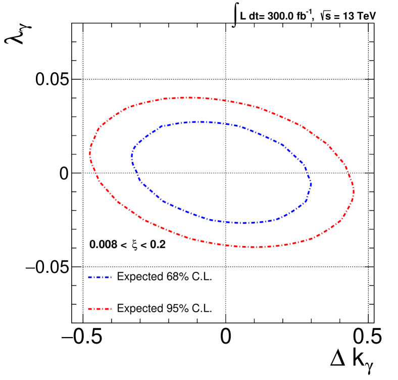
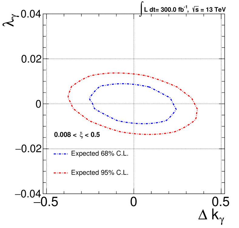
Figure 10: Two-dimensional 68$\%$ and 95$\%$ C.L. expected limit on the $\lambda_{\gamma}$ and $\Delta k_{\gamma}$ couplings assuming 0.008$<\xi<$0.2 (left) and 0.008$<\xi<$0.5 (right) and considering the IL corresponds to 300$\,{\rm fb}^{-1}$.

It is obvious that in the higher acceptance regions the sensitivity of the process to the anomalous parameters especially $\lambda_{\gamma}$ improve as the main contribution of the signal from this parameter appears at the high proton missing mass region. The one-dimensional 68$\%$ and 95$\%$ C.L. expected limits on these parameters are presented in Table 6 for both acceptance scenarios. It should be mentioned that since the $\Delta\kappa_{\gamma}$ contribution to the $W^{+}W^{-}\gamma$ CEP only increases the normalization of the SM, therefore, expected sensitivity of this parameter can be improved by lowering the mass cut criterion in Table 5. However, as in general the sensitivity of this process to the coupling$\Delta\kappa_{\gamma}$ is not high enough we decide to keep the same signal region for both couplings.

($\mathcal{L}=300\,{\rm fb}^{-1},\sqrt{s}=13{\rm\ TeV}$)
aTGCs	0.008$<\xi<$0.2	0.008$<\xi<$0.5
$\lambda_{\gamma}$	68$\%$ C.L. [-0.019,0.019]	68$\%$ C.L. [-0.006,0.006]
	95$\%$ C.L. [-0.032,0.032]	95$\%$ C.L. [-0.011,0.011,]
$\Delta\kappa_{\gamma}$	68$\%$ C.L. [-0.16,0.15]	68$\%$ C.L. [-0.17,0.16]
	95$\%$ C.L. [-0.26,0.25]	95$\%$ C.L. [0.30,0.29]

Table 6: 68$\%$ and 95$\%$ C.L expected limit on the $\lambda_{\gamma}$ and $\Delta k_{\gamma}$ couplings assuming two different acceptances, 0.008$<\xi<$0.2 and 0.008$<\xi<$0.5, considering the IL corresponds to 300$\,{\rm fb}^{-1}$.

7.3 Quartic gauge boson couplings

In this section, we examine the sensitivity of this process to the aQGCs arising from dimension-8 effective operators. It has been shown that the dimension-6 operators could contribute to both triple and quartic gauge boson couplings [62]. Therefore, the lowest order of operators which only appear as quartic couplings is dimension-8. Figure 11 shows the cross sections of $W^{+}W^{-}\gamma$ CEP as a function of four main new quartic couplings which give the contribution to this process via effective $WW\gamma\gamma$ vertex.

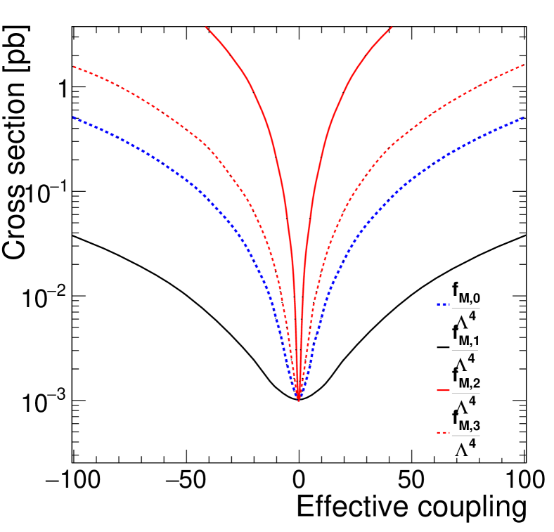
Figure 11: The cross sections of $\mathrm{p}\mathrm{p}\rightarrow\mathrm{p}W^{+}W^{-}\gamma\mathrm{p}$ as a function of four dimension-8 anomalous QGCs at proton-proton center-of-mass energy of 13 TeV.

As it can be seen $f_{M,2}$ and $f_{M,3}$ have strong dependency to the cross section and are expected to give tighter constraints comparing to the $f_{M,0}$ and $f_{M,1}$. Again in this section, we used the signal regions defined in Table 5. In the first step, we calculated the expected 68$\%$ and 95$\%$ C.L exclusion regions between two couplings for both acceptance scenarios. Figure 12 depicts these two dimensional allowed regions between $f_{M,1}$ and $f_{M,0}$ for acceptance of 0.008$<\xi<$0.2 (top-left) and 0.008$<\xi<$0.5 (top-right). The similar expected exclusion regions between $f_{M,3}$ and $f_{M,2}$ couplings for 0.008$<\xi<$0.2 (bottom-left) and 0.008$<\xi<$0.5 (bottom-right) are shown in Figure 12.

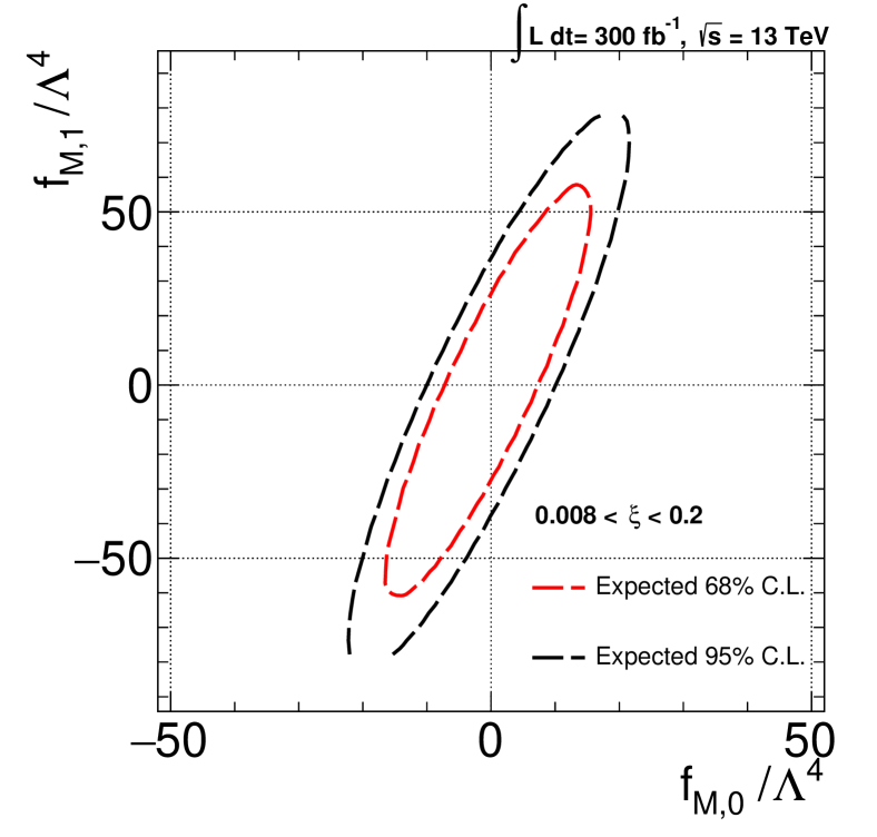
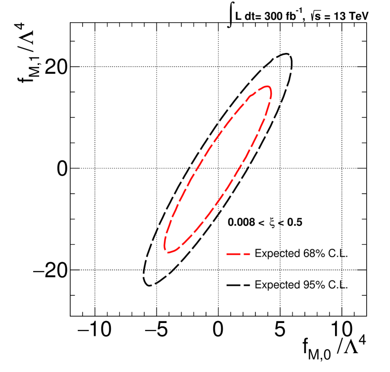
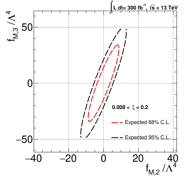
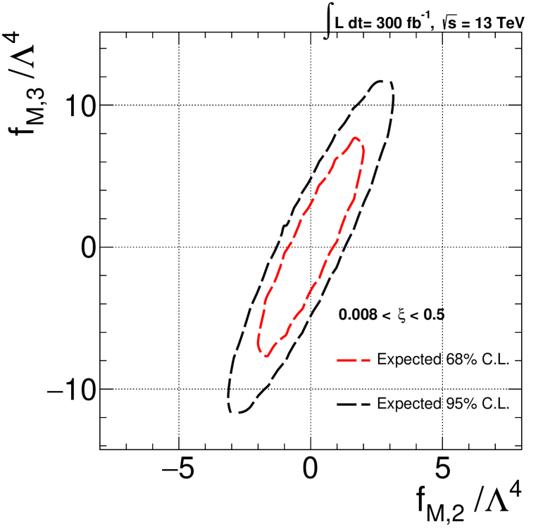
Figure 12: Two-dimensional 68$\%$ and 95$\%$ C.L expected allowed regions between $f_{M,1}$ and $f_{M,0}$ for acceptance of 0.008$<\xi<$0.2 (top-left) and 0.008$<\xi<$0.5 (top-right). Also Two-dimensional allowed region for $f_{M,3}$ and $f_{M,2}$ for acceptance of 0.008$<\xi<$0.2 (bottom-left) and 0.008$<\xi<$0.5 (bottom-right) assuming 300 f$\text{b}^{-1}$ IL.

We also estimate one-dimensional 68$\%$ and 95$\%$ C.L. expected limits on these anomalous couplings by assuming one coupling as free parameter and the rest couplings are set to zero. The one-dimensional constraints on aQGCs are presented in Table 7. The one-dimensional reported limit values in Table 7 include both acceptance scenarios, also considering the 300 $\text{fb}^{-1}$ IL.

68$\%$ and 95$\%$ Expected limit, ($\mathcal{L}=300\,{\rm fb}^{-1},\sqrt{s}=13{\rm\ TeV}$)
dimension-8 aQGC	0.008$<\xi<$0.2	0.008$<\xi<$0.5
$f_{M,0}/\Lambda^{4}({\rm\ TeV}^{-4})$	68$\%$ C.L. [-5.7,5.7]	68$\%$ C.L.[-1.3,1.3]
	95$\%$ C.L. [-8.7,8.7]	95$\%$ C.L. [-2.0,2.0]
$f_{M,1}/\Lambda^{4}({\rm\ TeV}^{-4})$	68$\%$ C.L. [-21.9,21.9]	68$\%$ C.L. [-5.0,5.0]
	95$\%$ C.L. [-32.8,32.8]	95$\%$ C.L. [-7.7,7.7]
$f_{M,2}/\Lambda^{4}({\rm\ TeV}^{-4})$	68$\%$ C.L. [-1.9,1.9]	68$\%$ C.L. [-0.5,0.5]
	95$\%$ C.L. [-3.2,3.2]	95$\%$ C.L. [-0.9,0.9]
$f_{M,3}/\Lambda^{4}({\rm\ TeV}^{-4})$	68$\%$ C.L. [-5.0,5.0]	68$\%$ C.L. [-1.2,1.2]
	95$\%$ C.L. [-7.9,7.9]	95$\%$ C.L. [-1.9,1.9]
$a_{0}^{W}/\Lambda^{2}({\rm\ TeV}^{-2})$	68$\%$ C.L. [-1.1,1.1]	68$\%$ C.L. [-0.3,0.3]
	95$\%$ C.L. [-1.8,1.8]	95$\%$ C.L. [-0.5,0.5]
$a_{C}^{W}/\Lambda^{2}({\rm\ TeV}^{-2})$	68$\%$ C.L. [-3.3,3.3]	68$\%$ C.L. [-0.8,0.8]
	95$\%$ C.L. [-5.2,5.2]	95$\%$ C.L. [-1.2,1.2]

Table 7: 68$\%$ and 95$\%$ C.L. expected limits on dimension-8 aQGCs assuming only one of them non-zero while the rest are set to zero. Expected limits on the dimension-6 aQGCs are also presented from translation of dimension-8 couplings. The limits include both acceptance scenarios and the 300 $\text{fb}^{-1}$ IL.

As it was explained in section 3 due to similar Lorentz structure of dimension-8 and dimension-6 operators they can be expressed in terms of each other which is shown in equation 3. Using this relation we translated limits on dimension-8 $f_{M,0,2}$ and $f_{M,1,3}$ anomalous couplings to the expected limit on dimension-6 $a_{0}^{W}$ and $a_{C}^{W}$ anomalous couplings which are shown in Table 7 for both assumed acceptance regions of protons. In addition, we calculated the expected allowed two-dimensional regions for $a_{0}^{W}$ and $a_{C}^{W}$ by generating the signal sample that includes the simultaneous variation of $f_{M,0,1,2,3}$ using the re-weighting approach implemented in the MadGraph5_aMC@NLO package  [64, 65]. By scanning the $f_{M,0,1,2,3}$ simultaneously over 400 points and translation of the expected limit on the $a_{0}^{W}$ and $a_{C}^{W}$ we obtain the two-dimensional 68$\%$ and 95$\%$ C.L. expected limit assuming the 300 f$\text{b}^{-1}$ IL shown in Figure 13 left and right for the acceptance regions of 0.008$<\xi<$0.2 and 0.008$<\xi<$0.5, respectively.

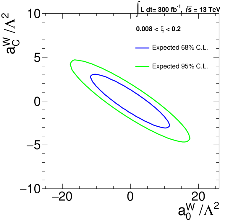
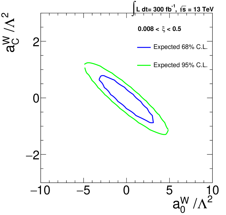
Figure 13: Two-dimensional 68$\%$ and 95$\%$ C.L. expected allowed regions of $a_{0}^{W}$ and $a_{C}^{W}$ for acceptance of 0.008$<\xi<$0.2 (left) and 0.008$<\xi<$0.5 (right), assuming 300 f$\text{b}^{-1}$ IL.

8 Summary and remarks

For the first time, the potential of the LHC to measure the CEP of $W^{+}W^{-}\gamma$ as well as the sensitivity of this process to the aTGCs and aQGCs, in the fully leptonic decay channel of W bosons, is explored. In contrast to the small predicted cross section of $W^{+}W^{-}\gamma$ CEP, this process is highly sensitive to multiple gauge boson couplings as the tree level diagrams made of purely gauge bosons.

To assess this goal first the feasibility of the LHC to measure the SM $W^{+}W^{-}\gamma$ production via quasi-real photon-photon scattering is investigated. The detailed understanding of final state objects both in the central and FDs are essential to distinguish signal process from the backgrounds. Signal events suffer from two major sources of background that arise from the other CEP processes with the common final state particles and inclusive processes which are coincided with the pile-up protons. Therefore, the presence of forward detectors with high resolution on momentum and arrival time of protons is vital to suppress background contributions. To preserve the optimum amount of signal also having maximum rejection of backgrounds we introduce three categories of selection cuts. The first set of cuts aims to keep the least number of objects needed to reconstruct the signal in the central detector. The second one reflects the acceptance limitations of FDs to tag intact protons. The final category of cuts benefits from the high kinematical correlation of central final state objects with the scattered protons detected by the FDs. The first and third type of cuts are very efficient for other CEP backgrounds such as $e^{+}e^{-}\gamma,\mu^{+}\mu^{-}\gamma,\tau^{+}\tau^{-}\gamma$ processes while all three categories of criterion are useful to reject the inclusive backgrounds which occur simultaneously with pile-up protons. The contribution of the latter background will grow as the mean number of pile-up increase in the high luminosity condition of the LHC. We evaluate the probability of tagging protons on FDs considering the energy acceptance and time of flight resolution w.r.t the vast range of mean pile-up scenarios from 10$-$140. The obtained probabilities can be used for any other studies aiming to estimate the contribution of inclusive backgrounds coincides with the pile-up protons. Then we estimate the amount of data that is needed to have strong evidence of SM predicted $W^{+}W^{-}\gamma$ central exclusive process and finally the observation of this process.

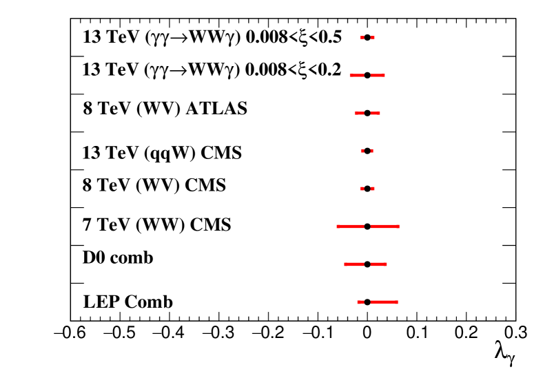
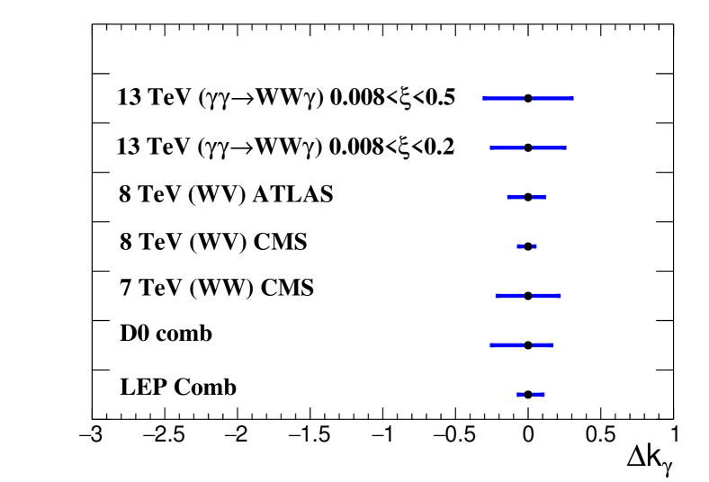
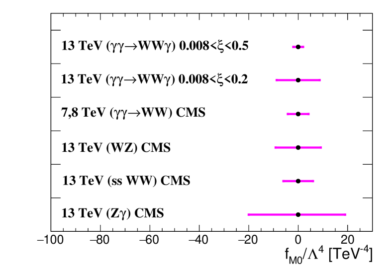
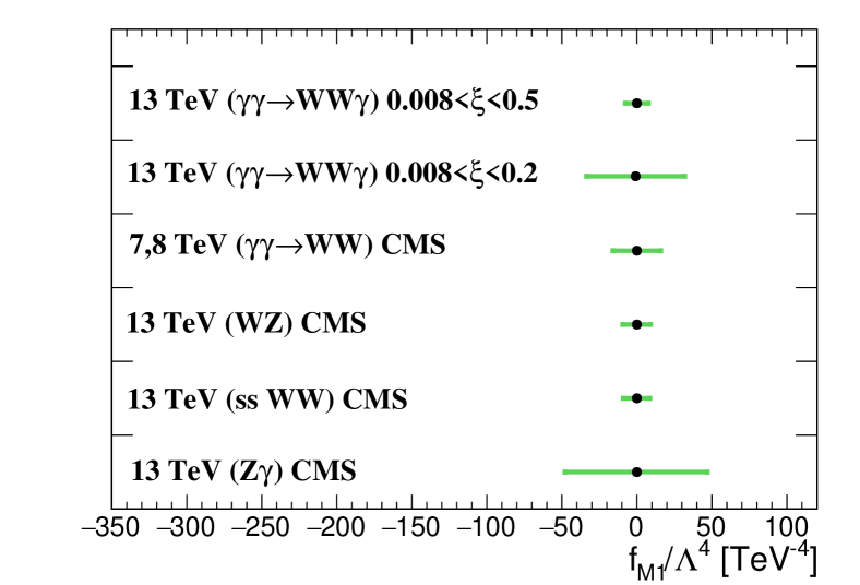
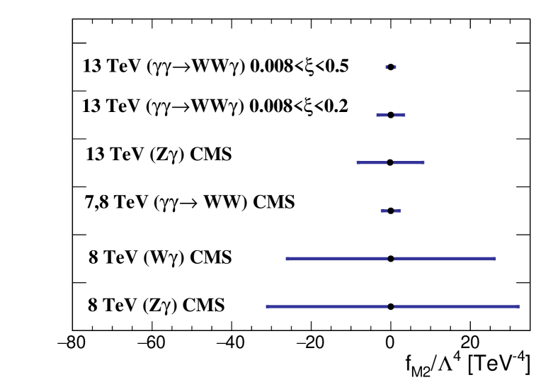
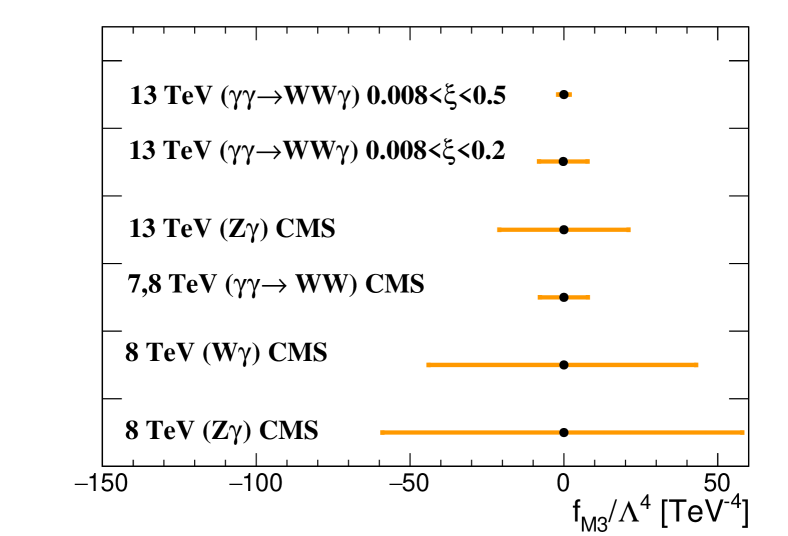
Figure 14: Comparison of expected 95$\%$ C.L. limit on aTGCs and aQGCs obtained from $\gamma\gamma\rightarrow WW\gamma$ analysis with center-of-mass energy of 13 TeV with current experimental observed limits [5, 6, 10, 11, 9, 15, 48, 12, 13, 8, 14]

In the second part, we estimate the power of this process to probe the aTGCs and aQGCs. In this regard, the $W^{+}W^{-}\gamma$ CEP also counts as irreducible background for the signal with anomalous couplings. As these anomalous couplings usually are emanated from momentum dependent terms in the effective Lagrangian. Therefore, the selection cuts introduced in the previous part upgraded to obtain the optimum signal region in the high momentum phase space. To study the new couplings, we consider the Lagrangian based on anomalous coupling approach for aTGCs. For aQGCs we employ dimension-8 effective terms that contribute to the $WW\gamma\gamma$ vertex. Then the expected limits are translated to the two dimension-6 operators contribute to the aQGCs. The expected 68$\%$ and 95$\%$ C.L. limit for all anomalous couplings are calculated individually. The two-dimensional limits are also extracted by obtaining the signal yields when two parameters vary simultaneously. All the limits are expressed in two considered acceptances of 0.008$<\xi<$0.2 and 0.008$<\xi<$0.5 for protons.

We have compared the obtained limits of this analysis with the current experimental bounds on aTGCs and aQGCs [5, 6, 10, 11, 9, 15, 48, 12, 13, 8, 14] which are shown in Figure 14. Left-top plot shows this process is highly sensitive to the $\lambda_{\gamma}$ while right-top plot indicates the obtained limits on $\Delta\kappa_{\gamma}$ are not competitive to the current bounds. This is partly because the high invariant mass cuts define the signal region while the $\Delta\kappa_{\gamma}$ coupling only alters the normalization of the SM process. Regarding the aQGCs, this analysis shows very good sensitivity to these couplings as it is obvious from left-middle, right-middle, left-bottom, and right-bottom plots which compare the expected limits on the $f_{M,0,1,2,3}$ to the current experimental observed limits by the CMS and ATLAS experiments, respectively. These plots show using $\gamma\gamma\rightarrow W^{+}W^{-}\gamma$ process one could obtain considerable improvement, especially on $f_{M,2}$ and $f_{M,3}$ couplings. Also, sensitivity on all four couplings is competitive with the inclusive $\gamma\gamma\rightarrow W^{+}W^{-}$ process measured by the CMS experiment [48]. In summary, this study shows the $W^{+}W^{-}\gamma$ CEP is very effective to probe the aQGCs and could be used by the current LHC experiments as a sensitive as well as a complementary channel to probe the multi-gauge boson couplings predicted in the SM.

Acknowledgments:

We are thankful to Christophe Royon and Mojtaba Mohammadi Najafabadi for insightful discussions and their helpful comments on the manuscript.

References

- [1] C. Degrande, N. Greiner, W. Kilian, O. Mattelaer, H. Mebane, T. Stelzer, S. Willenbrock and C. Zhang, Annals Phys. 335, 21 (2013) doi:10.1016/j.aop.2013.04.016 [arXiv:1205.4231 [hep-ph]].
- [2] W. Buchmuller and D. Wyler, Nucl. Phys. B 268, 621 (1986). doi:10.1016/0550-3213(86)90262-2
- [3] G. Belanger and F. Boudjema, Phys. Lett. B 288, 201 (1992). doi:10.1016/0370-2693(92)91978-I
- [4] M. Baak et al., arXiv:1310.6708 [hep-ph].
- [5] S. Schael et al. [ALEPH and DELPHI and L3 and OPAL and LEP Electroweak Collaborations], Phys. Rept. 532, 119 (2013) doi:10.1016/j.physrep.2013.07.004 [arXiv:1302.3415 [hep-ex]].
- [6] V. M. Abazov et al. [D0 Collaboration], Phys. Lett. B 718, 451 (2012) doi:10.1016/j.physletb.2012.10.062 [arXiv:1208.5458 [hep-ex]].
- [7] T. Aaltonen et al. [CDF Collaboration], Phys. Rev. D 86, 031104 (2012) doi:10.1103/PhysRevD.86.031104 [arXiv:1202.6629 [hep-ex]].
- [8] V. Khachatryan et al. [CMS Collaboration], JHEP 1706, 106 (2017) doi:10.1007/JHEP06(2017)106 [arXiv:1612.09256 [hep-ex]].
- [9] M. Aaboud et al. [ATLAS Collaboration], Eur. Phys. J. C 77, no. 8, 563 (2017) doi:10.1140/epjc/s10052-017-5084-2 [arXiv:1706.01702 [hep-ex]].
- [10] S. Chatrchyan et al. [CMS Collaboration], Eur. Phys. J. C 73, no. 10, 2610 (2013) doi:10.1140/epjc/s10052-013-2610-8 [arXiv:1306.1126 [hep-ex]].
- [11] A. M. Sirunyan et al. [CMS Collaboration], Phys. Lett. B 772, 21 (2017) doi:10.1016/j.physletb.2017.06.009 [arXiv:1703.06095 [hep-ex]].
- [12] A. M. Sirunyan et al. [CMS Collaboration], Phys. Lett. B 795, 281 (2019) doi:10.1016/j.physletb.2019.05.042 [arXiv:1901.04060 [hep-ex]].
- [13] A. M. Sirunyan et al. [CMS Collaboration], Phys. Rev. Lett. 120, no. 8, 081801 (2018) doi:10.1103/PhysRevLett.120.081801 [arXiv:1709.05822 [hep-ex]].
- [14] A. M. Sirunyan et al. [CMS Collaboration], arXiv:2002.09902 [hep-ex].
- [15] A. M. Sirunyan et al. [CMS Collaboration], Eur. Phys. J. C 80, no. 1, 43 (2020) doi:10.1140/epjc/s10052-019-7585-7 [arXiv:1903.04040 [hep-ex]].
- [16] V. M. Abazov et al. [D0 Collaboration], Phys. Rev. D 88, 012005 (2013) doi:10.1103/PhysRevD.88.012005 [arXiv:1305.1258 [hep-ex]].
- [17] G. Aad et al. [ATLAS Collaboration], Phys. Rev. Lett. 113, no. 14, 141803 (2014) doi:10.1103/PhysRevLett.113.141803 [arXiv:1405.6241 [hep-ex]].
- [18] M. Aaboud et al. [ATLAS Collaboration], Eur. Phys. J. C 77, no. 9, 646 (2017) doi:10.1140/epjc/s10052-017-5180-3 [arXiv:1707.05597 [hep-ex]].
- [19] S. Dawson, A. Likhoded, G. Valencia and O. Yushchenko, eConf C 960625, NEW147 (1996) [hep-ph/9610299].
- [20] R. Rahaman and R. K. Singh, arXiv:1711.04551 [hep-ph].
- [21] D. Choudhury and S. D. Rindani, Phys. Lett. B 335, 198 (1994) doi:10.1016/0370-2693(94)91413-3 [hep-ph/9405242].
- [22] B. Ananthanarayan, J. Lahiri, M. Patra and S. D. Rindani, JHEP 1408, 124 (2014) doi:10.1007/JHEP08(2014)124 [arXiv:1404.4845 [hep-ph]].
- [23] R. Rahaman and R. K. Singh, Eur. Phys. J. C 77, no. 8, 521 (2017) doi:10.1140/epjc/s10052-017-5093-1 [arXiv:1703.06437 [hep-ph]].
- [24] O. J. P. Eboli, M. C. Gonzalez-Garcia and S. F. Novaes, Nucl. Phys. B 411, 381 (1994) doi:10.1016/0550-3213(94)90455-3 [hep-ph/9306306].
- [25] B. Ananthanarayan, S. K. Garg, M. Patra and S. D. Rindani, Phys. Rev. D 85, 034006 (2012) doi:10.1103/PhysRevD.85.034006 [arXiv:1104.3645 [hep-ph]].
- [26] S. Y. Choi, Z. Phys. C 68, 163 (1995) doi:10.1007/BF01579815 [hep-ph/9412300].
- [27] S. Atag and I. Sahin, Phys. Rev. D 68, 093014 (2003) doi:10.1103/PhysRevD.68.093014 [hep-ph/0310047].
- [28] T. G. Rizzo, hep-ph/9907395.
- [29] P. Poulose and S. D. Rindani, Phys. Lett. B 452, 347 (1999) doi:10.1016/S0370-2693(99)00236-1 [hep-ph/9809203].
- [30] O. J. P. Eboli, M. B. Magro, P. G. Mercadante and S. F. Novaes, Phys. Rev. D 52, 15 (1995) doi:10.1103/PhysRevD.52.15 [hep-ph/9503432].
- [31] W. J. Stirling and A. Werthenbach, Eur. Phys. J. C 14, 103 (2000) doi:10.1007/s100520000399, 10.1007/s100520050737 [hep-ph/9903315].
- [32] G. Belanger, F. Boudjema, Y. Kurihara, D. Perret-Gallix and A. Semenov, Eur. Phys. J. C 13, 283 (2000) doi:10.1007/s100520000305 [hep-ph/9908254].
- [33] A. S. Belyaev, O. J. P. Eboli, M. C. Gonzalez-Garcia, J. K. Mizukoshi, S. F. Novaes and I. Zacharov, Phys. Rev. D 59, 015022 (1999) doi:10.1103/PhysRevD.59.015022 [hep-ph/9805229].
- [34] O. J. P. Eboli, M. C. Gonzalez-Garcia, S. M. Lietti and S. F. Novaes, Phys. Rev. D 63, 075008 (2001) doi:10.1103/PhysRevD.63.075008 [hep-ph/0009262].
- [35] O. J. P. Eboli, M. C. Gonzalez-Garcia and S. M. Lietti, Phys. Rev. D 69, 095005 (2004) doi:10.1103/PhysRevD.69.095005 [hep-ph/0310141].
- [36] U. Baur and D. L. Rainwater, Phys. Rev. D 62, 113011 (2000) doi:10.1103/PhysRevD.62.113011 [hep-ph/0008063].
- [37] M. Chiesa, A. Denner and J. N. Lang, Eur. Phys. J. C 78, no. 6, 467 (2018) doi:10.1140/epjc/s10052-018-5949-z [arXiv:1804.01477 [hep-ph]].
- [38] M. Chiesa, A. Denner and J. N. Lang, PoS LL 2018, 012 (2018) [arXiv:1808.03167 [hep-ph]].
- [39] E. Chapon, C. Royon and O. Kepka, Phys. Rev. D 81, 074003 (2010) doi:10.1103/PhysRevD.81.074003 [arXiv:0912.5161 [hep-ph]].
- [40] D. Yang, Y. Mao, Q. Li, S. Liu, Z. Xu and K. Ye, JHEP 1304, 108 (2013) doi:10.1007/JHEP04(2013)108 [arXiv:1211.1641 [hep-ph]].
- [41] S. M. Etesami, S. Khatibi and M. Mohammadi Najafabadi, Eur. Phys. J. C 76 (2016) no.10, 533 doi:10.1140/epjc/s10052-016-4376-2 [arXiv:1606.02178 [hep-ph]].
- [42] C. Bobeth and U. Haisch, JHEP 1509, 018 (2015) doi:10.1007/JHEP09(2015)018 [arXiv:1503.04829 [hep-ph]].
- [43] T. Corbett, O. J. P. Éboli, J. Gonzalez-Fraile and M. C. Gonzalez-Garcia, Phys. Rev. Lett. 111, 011801 (2013) doi:10.1103/PhysRevLett.111.011801 [arXiv:1304.1151 [hep-ph]].
- [44] B. Dumont, S. Fichet and G. von Gersdorff, JHEP 1307, 065 (2013) doi:10.1007/JHEP07(2013)065 [arXiv:1304.3369 [hep-ph]].
- [45] E. Masso, JHEP 1410, 128 (2014) doi:10.1007/JHEP10(2014)128 [arXiv:1406.6376 [hep-ph]].
- [46] M. Albrow et al. [CMS and TOTEM Collaborations], CERN-LHCC-2014-021, TOTEM-TDR-003, CMS-TDR-13.
- [47] S. Grinstein [AFP Collaboration], Nucl. Part. Phys. Proc. 273-275, 1180 (2016). doi:10.1016/j.nuclphysbps.2015.09.185
- [48] V. Khachatryan et al. [CMS Collaboration], JHEP 1608, 119 (2016) doi:10.1007/JHEP08(2016)119 [arXiv:1604.04464 [hep-ex]].
- [49] M. Aaboud et al. [ATLAS Collaboration], Phys. Rev. D 94, no. 3, 032011 (2016) doi:10.1103/PhysRevD.94.032011 [arXiv:1607.03745 [hep-ex]].
- [50] S. Chatrchyan et al. [CMS Collaboration], JHEP 1307, 116 (2013) doi:10.1007/JHEP07(2013)116 [arXiv:1305.5596 [hep-ex]].
- [51] A. Senol and M. Köksal, Phys. Lett. B 742, 143 (2015) doi:10.1016/j.physletb.2015.01.022 [arXiv:1410.3648 [hep-ph]].
- [52] T. Pierzchala and K. Piotrzkowski, Nucl. Phys. Proc. Suppl. 179-180, 257 (2008) doi:10.1016/j.nuclphysbps.2008.07.032 [arXiv:0807.1121 [hep-ph]].
- [53] R. S. Gupta, Phys. Rev. D 85, 014006 (2012) doi:10.1103/PhysRevD.85.014006 [arXiv:1111.3354 [hep-ph]].
- [54] S. Taheri Monfared, S. Fayazbakhsh and M. Mohammadi Najafabadi, Phys. Lett. B 762 (2016), 301-308 doi:10.1016/j.physletb.2016.09.055 [arXiv:1610.02883 [hep-ph]].
- [55] C. F. von Weizsacker, Z. Phys. 88, 612 (1934). doi:10.1007/BF01333110
- [56] E. J. Williams, Phys. Rev. 45, 729 (1934). doi:10.1103/PhysRev.45.729
- [57] V. M. Budnev, I. F. Ginzburg, G. V. Meledin and V. G. Serbo, Phys. Rept. 15, 181 (1975). doi:10.1016/0370-1573(75)90009-5
- [58] M. G. Albrow et al. [FP420 R and D Collaborations], JINST 4, T10001 (2009) doi:10.1088/1748-0221/4/10/T10001 [arXiv:0806.0302 [hep-ex]].
- [59] V. Avati and K. Osterberg. 2005. Report No. CERN-TOTEM-NOTE–002, (2006).
- [60] J. I. Djuvsland [ATLAS Collaboration], PoS EPS -HEP2017, 755 (2017). doi:10.22323/1.314.0755
- [61] O. J. P. Eboli, M. C. Gonzalez-Garcia and J. K. Mizukoshi, Phys. Rev. D 74, 073005 (2006) doi:10.1103/PhysRevD.74.073005 [hep-ph/0606118].
- [62] C. Degrande et al., arXiv:1309.7890 [hep-ph].
- [63] M. Baillargeon, G. Belanger and F. Boudjema, In *Paris 1994, Proceedings, Two-photon physics* 267-308, and Annecy Lab. Part. Phys. - ENSLAPP-A-473 (94/05,rec.May) 75 p [hep-ph/9405359].
- [64] J. Alwall, M. Herquet, F. Maltoni, O. Mattelaer and T. Stelzer, JHEP 1106, 128 (2011) doi:10.1007/JHEP06(2011)128 [arXiv:1106.0522 [hep-ph]].
- [65] J. Alwall et al., JHEP 1407, 079 (2014) doi:10.1007/JHEP07(2014)079 [arXiv:1405.0301 [hep-ph]].
- [66] A. Alloul, N. D. Christensen, C. Degrande, C. Duhr and B. Fuks, Comput. Phys. Commun. 185, 2250 (2014) doi:10.1016/j.cpc.2014.04.012 [arXiv:1310.1921 [hep-ph]].
- [67] C. Degrande, C. Duhr, B. Fuks, D. Grellscheid, O. Mattelaer and T. Reiter, Comput. Phys. Commun. 183, 1201 (2012) doi:10.1016/j.cpc.2012.01.022 [arXiv:1108.2040 [hep-ph]].
- [68] T. Sjostrand, S. Mrenna and P. Z. Skands, Comput. Phys. Commun. 178, 852 (2008) doi:10.1016/j.cpc.2008.01.036 [arXiv:0710.3820 [hep-ph]].
- [69] J. de Favereau et al. [DELPHES 3 Collaboration], JHEP 1402, 057 (2014) doi:10.1007/JHEP02(2014)057 [arXiv:1307.6346 [hep-ex]].
- [70] M. Cacciari, G. P. Salam and G. Soyez, JHEP 0804, 005 (2008) doi:10.1088/1126-6708/2008/04/005 [arXiv:0802.1188 [hep-ph]].
- [71] L. Adamczyk et al., CERN-LHCC-2015-009, ATLAS-TDR-024.
- [72] S. Nussinov, Phys. Rev. Lett. 34, 1286 (1975) doi:10.1103/PhysRevLett.34.1286
- [73] S. Nussinov, Phys. Rev. D 14, 246 (1976). doi:10.1103/PhysRevD.14.246
- [74] G. Ingelman and P. E. Schlein, Phys. Lett. 152B, 256 (1985). doi:10.1016/0370-2693(85)91181-5
- [75] R. Bonino et al. [UA8 Collaboration], Phys. Lett. B 211, 239 (1988). doi:10.1016/0370-2693(88)90840-4
- [76] T. Ahmed et al. [H1 Collaboration], Phys. Lett. B 348, 681 (1995) doi:10.1016/0370-2693(95)00279-T [hep-ex/9503005].
- [77] F. Abe et al. [CDF Collaboration], Phys. Rev. Lett. 79, 2636 (1997). doi:10.1103/PhysRevLett.79.2636
- [78] M. Boonekamp, A. Dechambre, V. Juranek, O. Kepka, M. Rangel, C. Royon and R. Staszewski, arXiv:1102.2531 [hep-ph].
- [79] A. D. Martin, V. A. Khoze and M. G. Ryskin, doi:10.3204/DESY-PROC-2009-02/15 arXiv:0810.3560 [hep-ph].
- [80] G. Cowan, K. Cranmer, E. Gross and O. Vitells, Eur. Phys. J. C 71, 1554 (2011) Erratum: [Eur. Phys. J. C 73, 2501 (2013)] doi:10.1140/epjc/s10052-011-1554-0, 10.1140/epjc/s10052-013-2501-z [arXiv:1007.1727 [physics.data-an]].
- [81] T. Corbett, O. J. P. Éboli and M. C. Gonzalez-Garcia, Phys. Rev. D 91, no. 3, 035014 (2015) doi:10.1103/PhysRevD.91.035014 [arXiv:1411.5026 [hep-ph]].
- [82] M. Aaboud et al. [ATLAS Collaboration], JHEP 1707, 107 (2017) doi:10.1007/JHEP07(2017)107 [arXiv:1705.01966 [hep-ex]].
- [83] V. Khachatryan et al. [CMS Collaboration], Phys. Lett. B 770, 380 (2017) doi:10.1016/j.physletb.2017.04.071 [arXiv:1702.03025 [hep-ex]].
- [84] A. M. Sirunyan et al. [CMS Collaboration], Phys. Lett. B 798, 134985 (2019) doi:10.1016/j.physletb.2019.134985 [arXiv:1905.07445 [hep-ex]].
- [85] S. S. Wilks, Annals Math. Statist. 9, no. 1, 60 (1938). doi:10.1214/aoms/1177732360