Local Graph Clustering with Network Lasso

Abstract

We study the statistical and computational properties of a network Lasso method for local graph clustering. The clusters delivered by nLasso can be characterized elegantly via network flows between cluster boundary and seed nodes. While spectral clustering methods are guided by a minimization of the graph Laplacian quadratic form, nLasso minimizes the total variation of cluster indicator signals. As demonstrated theoretically and numerically, nLasso methods can handle very sparse clusters (chain-like) which are difficult for spectral clustering. We also verify that a primal-dual method for non-smooth optimization allows to approximate nLasso solutions with optimal worst-case convergence rate.

I Introduction

Many application domains generate network structured data. Networked data arises in the study of self-organizing systems constituted by individual agents who can interact [21, 22]. Networked data also arises in computer vision where nodes represent individual pixels that are connected if they are close-by. Metrological observations collected by spatially distributed stations forms a network of time series with edges connecting close-by stations. We represent networked data conveniently using an “empirical” or “similarity” graph $\mathcal{G}$ [4, 30].

The analysis of networked data is often facilitated by grouping or clustering the data points into coherent subsets of data points. Clustering methods aim at finding subsets (clusters) of data points that are more similar to each other than to the remaining data points. Most existing clustering methods are unsupervised as they do not require the true cluster assignments for any data point [17, 19, 23, 30, 20, 18].

Local graph clustering starts from few “seed nodes” and explore their neighbourhoods to find clusters around them [29, 27]. With a runtime depending only on the resulting clusters, these methods are attractive for massive graphs [27, 8].

Spectral clustering methods use the eigenvectors of the graph Laplacian matrix to approximate the indicator functions of clusters [5, 26, 30, 23, 1]. These methods are computationally attractive as they amount to linear systems which can be implemented as scalable message passing protocols [7, 32]. Our approach differs from spectral clustering in the approximation of the cluster indicators.

To approximate cluster indicators, we use the solutions of a particular instance of the network Lasso (nLasso) optimization problem [9]. We solve this nLasso clustering problem using an efficient primal-dual method. This primal-dual method has attractive convergence guarantees and can be implemented as scalable message passing (see Section IV).

Building on our recent work on the duality between TV minimization and network flow optimization [14, 15], we show that the proposed nLasso clustering method can be interpreted (in a precise sense) as a flow-based clustering method [28, 31, 29, 16]. As detailed in Section III, our nLasso problem (and its dual flow optimization problem) is similar but different from the TV minimization problems (and its dual flow optimization problems) studied in [14, 15].

Compared with spectral methods, flow-based methods (including our approach) better handle sparsely connected (chain-like) clusters (see Section VI) and are more robust to “structural heterogeneities” [31, 11]. In contrast to existing flow-based local clustering methods, our approach is based on efficient convex optimization methods instead of computationally expensive combinatorial algorithms.

This paper makes the following contributions:

• Section II formulates local graph clustering as a particular instance of the nLasso problem.

• In Section III we derive the dual problem of the nLasso. We provide an interpretation of this dual problem as an instance of network flow optimization.

• Section IV presents a local clustering method by applying a primal-dual method to the nLasso problem. This method is appealing for big data applications as it can be implemented as a scalable message-passing method.

• Section V characterizes the clusters delivered by nLasso in terms of the amount of flow that can be routed from cluster boundaries to the seed nodes within that cluster. This offers a novel link between flow-based clustering and convex optimization.

II Local Graph Clustering

We consider networked data which is represented by a simple undirected weighted graph $\mathcal{G}=\big{(}\mathcal{V},\mathcal{E},\mathbf{W}\big{)}$. The nodes $\mathcal{V}=\{1,\ldots,n\}$ represent individual data points. Undirected edges $e=\{i,j\}\in\mathcal{E}$ connect similar data points $i,j\in\mathcal{V}$ and are assigned a positive weight $W_{i,j}\!>\!0$. Absence of an edge between nodes $i,j\!\in\!\mathcal{V}$ implies $W_{i,j}\!=\!0$. The neighbourhood of a node $i\!\in\!\mathcal{V}$ is $\mathcal{N}_{i}\!:=\!\{j\!\in\!\mathcal{V}:\{i,j\}\!\in\!\mathcal{E}\}$.

It will be convenient to define a directed version of the graph $\mathcal{G}$ by replacing each undirected edge $\{i,j\}$ by the directed edge $\big{(}{\rm min}\{i,j\},\max\{i,j\}\big{)}$. We overload notation and use $\mathcal{G}$ to denote the undirected and directed version of the empirical graph. The directed neighbourhoods of a node $i\in\mathcal{V}$ are

$$\mathcal{N}_{i}^{+}\!:=\!\{j\!\in\!\mathcal{V}\!:\!(i,j)\!\in\!\mathcal{E}\}\mbox{, and }\mathcal{N}_{i}^{-}\!:=\!\{j\!\in\!\mathcal{V}:(j,i)\!\in\!\mathcal{E}\}.$$ (1)

Local graph clustering starts from a given set of seed nodes

$$\mathcal{S}=\{i_{1},\ldots,i_{|S|}\}\subset\mathcal{V}.$$ (2)

The seed nodes might be obtained by exploiting domain knowledge and are grouped into batches $\mathcal{S}_{k}$,

$$\mathcal{S}=\mathcal{S}_{1}\cup\ldots\cup\mathcal{S}_{F}.$$ (3)

Each batch contains $L_{k}$ seed nodes of the same cluster $\mathcal{C}_{k}$.

We allow the number of seed nodes to be a vanishing fraction of the entire graph. This is an extreme case of semi-supervised learning where the labelling ratio (viewing seed nodes as labeled data points) goes to zero.

The proposed local graph clustering method (see Section 3) operates by exploring the neighbourhoods of the seed nodes $\mathcal{S}$. It constructs clusters $\mathcal{C}_{k}$ around the seed nodes $\mathcal{S}_{k}$ such that only few edges leave the cluster $\mathcal{C}_{k}$.

We characterize a cluster $\mathcal{C}_{k}$ via its boundary

$$\partial\mathcal{C}_{k}:=\{(i,j)\in\mathcal{E}:i\in\mathcal{C}_{k},j\notin\mathcal{C}_{k}\}.$$ (4)

A good cluster $\mathcal{C}_{k}$ is such that the total weight of the edges in its boundary $\partial\mathcal{C}_{k}$ is small. We make this characterization more precise in Section V using network flows to quantify the connectivity between cluster boundary and seed nodes.

III The Network Lasso and Its Dual

Local graph clustering methods learn graph signals $\hat{\mathbf{x}}\in\mathbb{R}^{\mathcal{V}}$ that are good approximations to the indicator signals $\mathbf{x}^{(k)}=\big{(}x_{1}^{(k)},\ldots,x_{n}^{(k)}\big{)}^{T}\in\mathbb{R}^{\mathcal{V}}$. These indicator signals represent the clusters $\mathcal{C}_{k}\subseteq\mathcal{V}$ around the seed nodes $\mathcal{S}_{k}$ (see (3)) via

$$x_{i}^{(k)}=\begin{cases}1&\mbox{ if }i\in\mathcal{C}_{k}\\ 0&\mbox{ otherwise.}\end{cases}.$$ (5)

Spectral graph clustering uses eigenvectors of the graph Laplacian matrix to approximations to cluster indicator signals. In contrast, we use TV minimization to learn approximations $\hat{\mathbf{x}}$ to the cluster indicators $\mathbf{x}^{(k)}$, for $k=1,\ldots,F$.

We have recently explored the relation between network flow problems and TV minimization [14, 15]. Loosely speaking, the solution of TV minimization is piece-wise constant over clusters whose boundaries have a small total weight. This property motivates us to learn the indicator function for the cluster $\mathcal{C}_{k}$ around the seed nodes $\mathcal{S}_{k}$ by solving

$$\hat{\mathbf{x}}\in\operatorname*{arg\;min}_{\mathbf{x}\in\mathbb{R}^{\mathcal{V}}}\sum_{i\in\mathcal{S}_{k}}(x_{i}\!-\!1)^{2}/2\!+\!\sum_{i\notin\mathcal{S}_{k}}\alpha x_{i}^{2}/2\!+\!\lambda\|\mathbf{x}\|_{\rm TV}.$$ (6)

Here, we used the total variation (TV)

$$\|\mathbf{x}\|_{\rm TV}=\sum_{\{i,j\}\in\mathcal{E}}W_{i,j}|x_{i}-x_{j}|.$$ (7)

Note that (6) is a non-smooth convex optimization problem. It is a special case of the nLasso problem [9].

We solve a separate nLasso problem (6) for each batch $\mathcal{S}_{k}$, for $k\!=\!1,\ldots,F$, of seed nodes in the same cluster. The nodes $i\!\notin\!\mathcal{S}_{k}$ which are not seed nodes for $\mathcal{C}_{k}$ belong to one of two groups. One group $\mathcal{C}_{k}\setminus\mathcal{S}_{k}$ of nodes which belong to $\mathcal{C}_{k}$ and the other group of nodes $i\notin\mathcal{C}_{k}$ outside the cluster.

The special case of (6) when $\alpha\!=\!0$ is studied in [14]. We can also interpret (6) as TV minimization using soft constraints instead of hard constraints [15]. While [15] enforces $\hat{x}_{i}$ for each seed node $i\in\mathcal{S}_{k}$, (6) uses soft constraints such that typically $\hat{x}_{i}\!<\!1$ at seed nodes $i\!\in\!\mathcal{S}_{k}$. Spectral methods use optimization problems similar to (6) but with the Laplacian quadratic form $\sum_{\{i,j\}\in\mathcal{E}}W_{i,j}(x_{i}\!-\!x_{j})^{2}$ instead of TV (7).

We hope that any solution to (6) is a good approximation to the indicator function $x^{(k)}$ of a well-connected subset around the seed nodes $\mathcal{S}_{k}$. We use the graph signal $\hat{x}:i\mapsto\hat{x}_{i}$ obtained from solving (6) to determine a reasonable cluster $\mathcal{C}_{k}\!\supseteq\!\mathcal{S}_{k}$.

The idea of determining clusters via learning graph signals as (approximations) of indicator functions of good clusters is also underlying spectral clustering [30]. Instead of TV minimization underlying nLasso (6), spectral clustering uses the matrix Laplacian to score candidates for cluster indicator functions. Moreover, spectral clustering methods do not require any seed nodes with known cluster assignment.

The choice of the tuning parameters $\alpha$ and $\lambda$ in (6) crucially influence the behaviour of the clustering method and the properties of clusters delivered by (6). Their choice can be based on the intuition provided by a minimum cost flow problem that is dual (equivalent) to nLasso (6). This minimum cost flow problem is not defined directly on the empirical graph $\mathcal{G}$ but the augmented graph $\widetilde{\mathcal{G}}=\big{(}\widetilde{\mathcal{V}},\widetilde{\mathcal{E}}\big{)}$. This augmented graph is obtained by augmenting the graph $\mathcal{G}$ with an additional node “$\star$” and edges $(i,\star)$ for each node $i\in\mathcal{V}$.

As detailed in the supplementary material, the nLasso (6) is equivalent (dual) to the minimum cost flow problem [15, 14]

$$\min_{y\in\mathbb{R}^{\mathcal{E}}}\sum_{i\in\mathcal{S}_{k}}(y_{(i,\star)}-1)^{2} +(1/\alpha)\sum_{i\notin\mathcal{S}_{k}}y_{(i,\star)}^{2}$$ (8)

$$\mbox{s.t.}\sum_{j\in\mathcal{N}_{i}^{+}}y_{(i,j)} =\sum_{j\in\mathcal{N}_{i}^{-}}y_{(j,i)}\mbox{for all nodes }i\in\widetilde{\mathcal{V}}$$ (9)

$$|y_{e}| \leq\lambda W_{e}\mbox{ for all }e\in\mathcal{E}.$$ (10)

The constraints (9) enforce conservation of the flow $y_{e}$ at every node $i\!\in\!\widetilde{\mathcal{V}}$. The constrains (10) enforce the flow $y_{e}$ not exceeding the edge capacity $\lambda W_{e}$. There are no capacity constrains for augmented edges $(i,\star)$ with $i\!\in\!\mathcal{V}$.

The node signal $\hat{\mathbf{x}}$ solves (6) and the edge signal $\hat{\mathbf{y}}$ solve (8), respectively, if and only if [25, Ch. 31]

$$-\sum_{j\in\mathcal{N}_{i}^{+}}\hat{y}_{(i,j)}+\sum_{j\in\mathcal{N}_{i}^{-}}\hat{y}_{(j,i)} =\hat{x}_{i}\!-\!1\mbox{ for }i\in\mathcal{S}_{k}$$ (11)

$$-\sum_{j\in\mathcal{N}_{i}^{+}}\hat{y}_{(i,j)}+\sum_{j\in\mathcal{N}_{i}^{-}}\hat{y}_{(j,i)} =\alpha\hat{x}_{i}\mbox{ for }i\notin\mathcal{S}_{k}$$ (12)

$$|\hat{y}_{e}|\leq\lambda W_{e}\mbox{ for all edges }e\in\mathcal{E}$$ (13)

$$\hat{x}_{i}\!-\!\hat{x}_{j}\!=\!0\mbox{ for }e\!=\!(i,j)\in\mathcal{E}\mbox{ with }|\hat{y}_{(i,j)}|\!<\!\lambda W_{e}.$$ (14)

We can interpret conditions (11), (12) as conservation laws satisfied by any flow $\hat{y}_{e}$ that solves the nLasso dual (8). We can think of injecting (extracting) a flow of value $\hat{x}_{i}\!-\!1$ at seed nodes $i\!\in\!\mathcal{S}_{k}$. The nodes $i\notin\mathcal{S}_{k}$ are leaking a flow of value $\alpha\hat{x}_{i}$. The optimal flow $\hat{y}_{e}$ has to provide these demands while respecting the capacity constraints (13).

We illustrate the conditions (11)-(14) in Fig. 1 for a simple chain graph. According to (14), the nLasso solution $\hat{\mathbf{x}}$ can only change across edges $e=(i,j)$ which are saturated $|\hat{y}_{e}|=\lambda W_{e}$. For a chain graph, using a suitable choice for $\alpha$ and $\lambda$ in (6), nLasso is able to recover a cluster structure as soon as the weights of boundary edges exceeds the weights of intra-cluster edges.

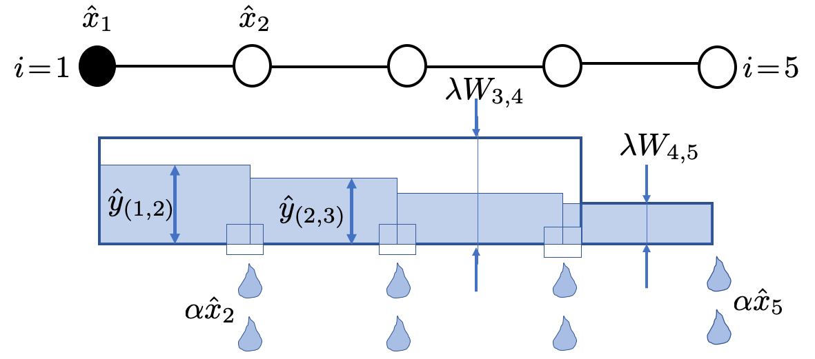
Figure 1: The dual (8) of nLasso optimizes the flow through a leaky network obtained from the empirical graph $\mathcal{G}$.

We use the optimality condition (11)-(14) to characterize the solutions of nLasso (6) in Section V. Combining this characterization with generative models for the clusters $\mathcal{C}_{k}$, such as stochastic block models, allows to derive sufficient conditions on the parameters of the generative model such that solutions of (6) allow to recover the true underlying local clusters [13].

IV Computational Aspects

The necessary and sufficient conditions (11)-(14) characterize any pair of solutions for (6) and its dual (8). We can find solutions to the conditions (11)-(14), which provides a solution to nLasso in turn, by reformulating those coupled condition as a fixed point equation.

There are many different fixed-point equations that are equivalent to the optimality conditions (11)-(14). We will use a particular construction which results in a method that is guaranteed to converge to a solution of (6) and (8) and can be implemented as a scalable message passing on the empirical graph $\mathcal{G}$. This construction is discussed in great detail in [2] and has been applied to the special case of nLasso (6) for $\alpha=0$ in our recent work [14]. For local graph clustering, we need $\alpha>0$ to force the solutions of (6) to decay towards zero outside the local cluster around the seed nodes $\mathcal{S}_{k}$.

Applying tools from [14], we obtain the following updates generating two sequences $\hat{x}_{i}^{(r)}$ and $\hat{y}_{e}^{(r)}$, for $r=0,1,\ldots$, converging to solutions of (6) and (8), respectively.

$$\vspace*{-2mm}\tilde{x}_{i} \!:=\!2\hat{x}^{(r)}_{i}-\hat{x}^{(r\!-\!1)}_{i}\mbox{ for }i\!\in\!\mathcal{V}$$ (15)

$$\hat{y}^{(r\!+\!1)}_{e} \!:=\!\hat{y}^{(r)}_{e}\!+\!(1/2)(\tilde{x}_{i}\!-\!\tilde{x}_{j})\mbox{ for }e=(i,j)\!\in\!\mathcal{E}$$ (16)

$$\hat{y}^{(r\!+\!1)}_{e} \!:=\!\hat{y}_{e}^{(k\!+\!1)}\!/\!\max\{1,|\hat{y}_{e}^{(r\!+\!1)}|/(\lambda W_{e})\}\mbox{ for }(i,j)\!\in\!\mathcal{E}$$ (17)

$$\hat{x}^{(r\!+\!1)}_{i} \!:=\!\hat{x}^{(r)}_{i}\!-\!\gamma_{i}\bigg{[}\sum_{j\!\in\!\mathcal{N}_{i}^{+}}\hat{y}^{(r\!+\!1)}_{(i,j)}\!-\!\sum_{j\!\in\!\mathcal{N}_{i}^{-}}\hat{y}^{(r\!+\!1)}_{(j,i)}\bigg{]}\mbox{ for }i\!\in\!\mathcal{V}$$ (18)

$$\hat{x}_{i}^{(r\!+\!1)} \!:=\!\big{(}\gamma_{i}\!+\!\hat{x}^{(r\!+\!1)}_{i}\big{)}/(\gamma_{i}\!+\!1)\mbox{ for every }i\!\in\!\mathcal{S}_{k}$$ (19)

$$\hat{x}_{i}^{(r\!+\!1)} \!:=\!\hat{x}^{(r\!+\!1)}_{i}/(\alpha\gamma_{i}\!+\!1)\mbox{ for every }i\!\in\!\mathcal{V}\setminus\mathcal{S}_{k}.$$ (20)

Here, $\gamma_{i}=1/d_{i}$ is the inverse of the node degree $d_{i}=\big{|}\mathcal{N}_{i}\big{|}$. Starting from an arbitrary initialization $\hat{x}^{(0)}_{i}$ and $\hat{y}^{(0)}_{e}$, the iterates $\hat{x}^{(r)}_{i}$ and $\hat{y}^{(r)}_{e}$ converge to a solution of nLasso (6) and its dual (8), respectively [10].

The updates (15)-(20) define a message-passing on the empirical graph $\mathcal{G}$ to jointly solve nLasso (6) and its dual (8). The computational complexity of one full iteration is proportional to the number of edges in the empirical graph. The overall complexity also depends on the number of iterations required to ensure the iterate $\hat{x}_{i}^{(r)}$ being sufficiently close to the nLasso (6) solution.

Basic analysis of proximal methods shows that the number of required iterations required scales inversely with the required sub-optimality of $\hat{x}_{i}^{(r)}$ (see [3, 6]). This convergence rate cannot be improved for chain graphs [12]. For a fixed number of iterations and empirical graphs with bounded maximum node degree, the computational complexity of our method scales linearly with the number of nodes (data points).

We now develop an interpretation of the updates (15)-(20) as an iterative method for network flow optimization. The update (17) enforces the capacity constraints (10) to be satisfied for the flow iterates $\hat{y}^{(r)}$. The update (18) amounts to adjusting the current nLasso estimate $\hat{x}_{i}^{(r)}$, for each node $i\in\!\mathcal{V}$ by the demand induced by the current flow approximation $\hat{y}^{(r)}$.

Together with the updates (19) and (20), the update (18) enforces the flow $\hat{y}^{(r)}$ to satisfy the conservation laws (11) and (12). The update (16) aims at enforcing (14) by adjusting the cumulated demands $\hat{x}^{(r)}_{i}$ via the flow $\hat{y}^{(r)}_{(i,j)}$ through an edge $e=(i,j)\in\mathcal{E}$ according to the difference $(\tilde{x}_{i}-\tilde{x}_{j})$.

The above interpretation helps to guide the choice for the parameters $\alpha$ and $\lambda$ in (6). The edge capacities $\lambda W_{e}$ limit the rate by which the values $\hat{x}^{(r)}_{i}$ can be “build up”. Choosing $\lambda$ too small would, therefore, slow down the convergence of $\hat{x}^{(r)}_{i}$. On the other hand, using nLasso (6) with too large $\lambda$ does not allow to detect small local clusters $\mathcal{C}_{k}$ (see Section V).

V Cluster Characterization

We use the solution $\hat{x}_{i}$ of nLasso (6) to approximate the indicator of a local cluster around the seed nodes $\mathcal{S}_{k}$. The cluster delivered by our method is obtained by thresholding,

$$\mathcal{C}_{k}:=\{i\in\mathcal{V}:\hat{x}_{i}>1/2\}.$$ (21)

In practice we replace the exact nLasso solution $\hat{x}_{i}$ in (21) with the iterate $\hat{x}^{(r)}_{i}$ obtained after a sufficient number $r$ of primal-dual updates (15)-(20) (see Section VI). The threshold $1/2$ is (21) is somewhat arbitrary. Our theoretical results can be easily adapted for other choices for the threshold. The question if there exists an optimal choice for the threshold and what this actually means precisely is beyond the scope of this paper.

Our main theoretical result is a necessary condition on the cluster (21) and the nLasso parameters $\alpha$ and $\lambda$ (see (6)).

Proposition 1.

Consider the cluster (21) obtained from the nLasso solution. Then, if $\mathcal{S}_{k}\subseteq\mathcal{C}_{k}$,

$$\lambda\sum_{e\in\partial\mathcal{C}_{k}}W_{e}\leq 1-(\alpha/2)\sum_{i\in\mathcal{C}_{k}\setminus\mathcal{S}_{k}}\hat{x}^{(r)}_{i}.$$ (22)

and

$$\lambda\sum_{e\in\partial\mathcal{C}_{k}}W_{e}\leq\alpha\sum_{i\notin\mathcal{C}_{k}}\hat{x}^{(r)}_{i}.$$ (23)

Proof.

Follows from the optimality conditions (11)-(14). ∎

The necessary conditions (22) and (23) can guide the choice of the parameters $\alpha$ and $\lambda$ in (6). We can enforce nLasso to deliver clusters with small boundary $\partial\mathcal{C}_{k}$ by using a a large $\lambda$ in (6). Since the left side of (22) must not exceed the right hand side, using a large $\lambda$ enforces a cluster (21) such that $\sum_{e\in\partial\mathcal{C}_{k}}W_{e}$ is small. In the extreme case of very large $\lambda$, this leads to $\partial\mathcal{C}_{k}$ being empty. There is a critical value for $\lambda$ in (6) beyond which the cluster $\mathcal{C}_{k}$ (21) contains all connected components with seed nodes $\mathcal{S}_{k}$.

We can combine (23) with an upper bound $U$ on the number of nodes $i\notin\mathcal{C}_{k}$ reached by message-passing updates (15)-(20). Inserting this bound $U$ on the number of “relevant” nodes $i\notin\mathcal{C}_{k}$ into (23), yields the necessary condition

$$\lambda\sum_{e\in\partial\mathcal{C}_{k}}W_{e}\leq U\alpha/2.$$ (24)

VI Numerical Experiments

We verify Proposition 1 numerically on a chain graph $\mathcal{G}_{c}$ with nodes $\mathcal{V}\!=\!\{1,\ldots,100\}$. Consecutive nodes $i$ and $i\!+\!1$ are connected by edges of weight $W_{e}\!=\!5/4$ with the exception of edge $e^{\prime}=\{4,5\}$ with the weight $W_{e^{\prime}}\!=\!1$.

We determine a cluster $\mathcal{C}_{1}$ around seed node $i\!=\!1$ using (21). The updates (15)-(20) are iterated for a fixed number of $K\!=\!1000$ iterations. The nLasso parameters were set to $\lambda\!=\!2/10$ and $\alpha\!=\!1/200$ (see (6)). These parameter values ensure conditions (22) and (24) (with $U\!=\!80$) are satisfied for the resulting cluster is $\mathcal{C}_{1}=\{1,2,3,4\}$.

We depict the resulting graph signal $\hat{x}^{(K)}_{i}$ (“$\circ$”) for the first $20$ nodes of $\mathcal{G}_{c}$ in Fig. 2. We also show the (scaled) eigenvector (“$\star$”) of the graph Laplacian corresponding to the smallest non-zero eigenvalue. This eigenvector is known as the Fiedler vector and used by spectral graph clustering methods to approximate the cluster indicators [24]. According to Fig. 2, the (approximate) nLasso solution better approximates the indicator of the true cluster $\mathcal{C}_{1}=\{1,2,3,4\}$.

Figure 2: Signal (“$\circ$”) obtained after $1000$ iterations of (15)-(20) for the chain graph $\mathcal{G}_{c}$ . The resulting local cluster is $\mathcal{C}_{1}\!=\!\{1,2,3,4\}$ (see (21)). We also depict the graph signal (“$\star$”) obtained by the eigenvector of the normalized graph Laplacian corresponding to the smallest non-zero eigenvalue.

In a second experiment, we compare our method with existing local clustering methods in a simple image segmentation task. We represent an image as a grid graph whose nodes are individual pixels. Vertically and horizontally adjacent pixels are connected by edges with weight $W_{i,j}=\exp(-(g_{i}-g_{j})^{2}/20^{2})$ with the greyscale value $g_{i}\in\{0,\dots,255\}$ of the $i$-th pixel.

We determine a local cluster around a set of seed nodes (see Fig. 3(a)) using $K=1000$ iterations of (15)-(20) to approximately solve nLasso (6) (see Fig. 3(b)). The local cluster obtained by the flow-based capacity releasing diffusion (CRD) method [31] is depicted in Fig. 3(c). The local clustering obtained by the spectral method presented in [1] is shown in Fig. 3(d). The seed nodes and resulting clusters obtained by the three methods are enclosed by a red contour line in Fig. 3. It seems that our method is the only method which can accurately determine the pixels belonging to the foreground object (a coin) around the seed nodes (see Fig. 3(a)).

A third experiment compares our method with existing clustering methods for an empirical graph being the realization of a partially labelled stochastic block model (SBM). We used a SBM with two blocks or clusters $\mathcal{C}_{1}$ and $\mathcal{C}_{2}$. Each cluster consists of $100$ nodes. A randomly chosen pair of nodes is connected by an edge with probability $1/5$ ($1/100$) if they belong to the same block (different blocks). The cluster (21) delivered by nLasso (6), with $\alpha=1/40$ and $\lambda=1/200$ and using $20$ randomly chosen seed nodes, perfectly recovered the true clusters. The spectral method [1] achieved labelling accuracy (fraction of correctly labelled nodes) of $1/2$. The flow-based methods [31, 16] achieved a labelling accuracy of around $9/10$.

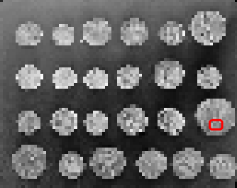
(a) Image with seed nodes.

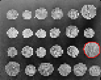
(b) nLasso (6).

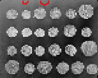
(c) Flow-based CRD [31].

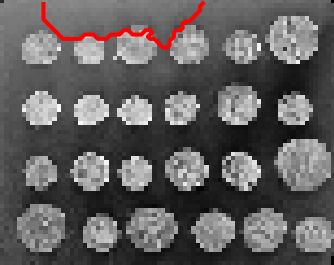
(d) Approximate Page-Rank [1].

Figure 3: Image segmentation results.

The source code for the above experiments can be found at https://github.com/alexjungaalto/.

VII Conclusion

We have studied the application of nLasso to local graph clustering. Our main technical result is a characterization of the nLasso solutions in terms of network flows between cluster boundaries and seed nodes. Conceptually, we provide an interesting link between flow-based clustering and non-smooth convex optimization. This work offers several avenues for follow-up research. We have recently proposed networked exponential families to couple the network topology with the information geometry of node-wise probabilistic models. It is interesting to study how the properties of these node-wise probabilistic models can be exploited to guide local clustering methods.

VIII Supplementary Material

Duality of nLasso (6) and Minimum Cost Flow (8). Let us rewrite nLasso (6) as

$$\min_{\mathbf{x}\in\mathbb{R}^{\mathcal{V}}}f(\mathbf{x})+g(\mathbf{B}\mathbf{x})$$ (25)

with the unweighted incidence matrix $\mathbf{B}$ of $\mathcal{G}$. For some edge $e\!\in\!\mathcal{E}$ and node $i\!\in\!\mathcal{V}$, $B_{e,i}\!=\!1$ if $e\!=\!(i,j)$ for some $j\!\in\!\mathcal{V}$, $B_{e,i}\!=\!-1$ if $e\!=\!(j,i)$ for some $j\!\in\!\mathcal{V}$ and $B_{e,i}=0$ otherwise.

The components in (25) are

$$f(\mathbf{x})\!:=\!\sum_{i\in\mathcal{S}_{k}}(x_{i}\!-\!1)^{2}/2\!+\!\sum_{i\notin\mathcal{S}_{k}}\alpha x_{i}^{2}/2\mbox{, }g(\mathbf{y})\!:=\!\lambda\sum_{e\in\mathcal{E}}W_{e}|y_{e}|.$$ (26)

According to [25, Cor. 31.2.1] (see also [3, Sec. 3.5]),

$$\min_{\mathbf{x}\in\mathbb{R}^{\mathcal{V}}}f(\mathbf{x})+g(\mathbf{B}\mathbf{x}) =\max_{\mathbf{y}\in\mathbb{R}^{\mathcal{E}}}-g^{*}(-\mathbf{y})-f^{*}(\mathbf{B}^{T}\mathbf{y})$$

$$=\max_{\mathbf{y}\in\mathbb{R}^{\mathcal{E}}}-g^{*}(\mathbf{y})-f^{*}(-\mathbf{B}^{T}\mathbf{y})$$ (27)

with the convex conjugates

$$g^{*}(\mathbf{y}) :=\sup_{\mathbf{z}\in\mathbb{R}^{\mathcal{E}}}\mathbf{y}^{T}\mathbf{z}-g(\mathbf{z})\stackrel{{\scriptstyle\eqref{equ_f_g_primal_dual_proof}}}{{=}}\sup_{\mathbf{z}\in\mathbb{R}^{\mathcal{E}}}\mathbf{y}^{T}\mathbf{z}-\lambda\sum_{e\in\mathcal{E}}W_{e}|z_{e}|$$

$$=\begin{cases}\infty&\text{if $|y_{e}|>\lambda W_{e}\mbox{ for some }e\in\mathcal{E}$}\\ 0&\text{otherwise}\end{cases}$$ (28)

and

$$f^{*}(\mathbf{x}) \!:=\sup_{\mathbf{w}\in\mathbb{R}^{\mathcal{V}}}\mathbf{x}^{T}\mathbf{w}-f(\mathbf{w})$$ (29)

$$~\stackrel{{\scriptstyle\eqref{equ_f_g_primal_dual_proof}}}{{=}}\sup_{\mathbf{w}\in\mathbb{R}^{\mathcal{V}}}\sum_{i\in\mathcal{S}_{k}}\big{[}x_{i}w_{i}\!-\!(1/2)(w_{i}\!-\!1)^{2}\big{]}\!+\!\sum_{i\notin\mathcal{S}_{k}}\big{[}x_{i}w_{i}\!-\!(\alpha/2)w^{2}_{i}\big{]}.$$

Exploiting the separability of the supremum in (29),

$$f^{*}(\mathbf{z})=\sum_{i\in\mathcal{S}_{k}}\left((1/2)z_{i}^{2}+z_{i}\right)+\sum_{i\notin\mathcal{S}_{k}}(1/2\alpha)z_{i}^{2}.$$ (30)

Using (30) and (VIII) allows to rewrite the RHS of (VIII) as

$$\max_{\mathbf{x}\in\mathbb{R}^{\mathcal{V}},\mathbf{y}\in\mathbb{R}^{\mathcal{E}}} -\sum_{i\in\mathcal{S}_{k}}\left((1/2)x_{i}^{2}-x_{i}\right)-\sum_{i\notin\mathcal{S}_{k}}(1/2\alpha)x_{i}^{2}$$

$$\mbox{ s.t.\ }x_{i}\!=\!\sum_{j\in\mathcal{N}^{+}_{i}}y_{i,j}\!-\!\sum_{j\in\mathcal{N}^{-}_{i}}y_{j,i}\mbox{, }i\!\in\!\mathcal{V}\mbox{, }|y_{e}|\!\leq\!\lambda W_{e}\mbox{, }e\!\in\!\mathcal{E}.$$ (31)

Since maximizing some real-valued function $t(\cdot)$ is equivalent to minimizing $-t(\cdot)$, the optimization problem (31) is equivalent to

$$\min_{\mathbf{x}\in\mathbb{R}^{\mathcal{V}},\mathbf{y}\in\mathbb{R}^{\mathcal{E}}} \sum_{i\in\mathcal{S}_{k}}\left((1/2)x_{i}^{2}-x_{i}\right)+\sum_{i\notin\mathcal{S}_{k}}(1/2\alpha)x_{i}^{2}$$

$$\mbox{ s.t.\ }x_{i}\!=\!\sum_{j\in\mathcal{N}^{+}_{i}}y_{i,j}\!-\!\sum_{j\in\mathcal{N}^{-}_{i}}y_{j,i}\mbox{, }i\!\in\!\mathcal{V}\mbox{, }|y_{e}|\!\leq\!\lambda W_{e}\mbox{, }e\!\in\!\mathcal{E}.$$ (32)

Primal-Dual Optimality Condition (11)-(14). Consider the primal form (25) of the nLasso (6) and the corresponding dual problem on the RHS of (VIII). According to [25, Thm. 31.3], the graph signal $\hat{\mathbf{x}}$ solves (25) and the edge signal $\hat{\mathbf{y}}$ solves (8), respectively, if and only if,

$$-\mathbf{B}^{T}\hat{\mathbf{y}}\in\partial f(\hat{\mathbf{x}})\mbox{ , and }\mathbf{B}\hat{\mathbf{x}}\in\partial g^{*}(\hat{\mathbf{y}}).$$ (33)

The second condition in (33) is equivalent to (13)-(14). This equivalence can be verified by evaluating the sub-differential of $g^{*}(\mathbf{y})=\max_{e\in\mathcal{E}}g^{*}(y_{e})$ (see Figure 4). The first condition in (33) is equivalent to (11) and (12) since $\frac{\partial f(\mathbf{x})}{\partial x_{i}}=x_{i}-1$ for $i\in\mathcal{S}_{k}$ and $\frac{\partial f(\mathbf{x})}{\partial x_{i}}=\alpha x_{i}$ for $i\in\mathcal{V}\setminus\mathcal{S}_{k}$.

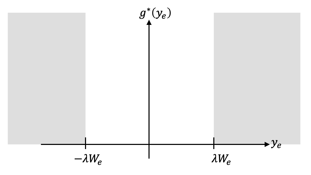
Figure 4: Components $g^{*}(y_{e})$ of convex conjugate $g^{*}(\mathbf{y})$.

References

- [1] R. Andersen, F. Chung, and K. Lang. Local graph partitioning using pagerank vectors. In Proc. 47th Annual IEEE Symp. Found. Computer Science, pages 475–486, Oct. 2006.
- [2] A. Chambolle and T. Pock. A first-order primal-dual algorithm for convex problems with applications to imaging. J. Math. Imag. Vis., 40(1), 2011.
- [3] A. Chambolle and T. Pock. An introduction to continuous optimization for imaging. Acta Numer., 25:161–319, 2016.
- [4] O. Chapelle, B. Schölkopf, and A. Zien, editors. Semi-Supervised Learning. The MIT Press, Cambridge, Massachusetts, 2006.
- [5] F. R.K̃. Chung. Spectral Graph Theory. 1997.
- [6] P. L. Combettes and J.-C. Pesquet. Proximal splitting methods in signal processing. In H. Bauschke, R. Burachik, P. Combettes, V. Elser, D. Luke, and H. Wolkowicz, editors, Fixed-Point Algorithms for Inverse Problems in Science and Engineering, volume 49. Springer New York, 2011.
- [7] A. G. Dimakis, S. Kar, J. M. F. Moura, M. G. Rabbat, and A. Scaglione. Gossip algorithms for distributed signal processing. Proceedings of the IEEE, 98(11):1847–1864, Nov. 2010.
- [8] K. Fountoulakis, D. F. Gleich, and M. W. Mahoney. A short introduction to local graph clustering methods and software. In The 7th Int. Conf. Compl. Networks and App., Cambridge, UK, Dec. 2018.
- [9] D. Hallac, J. Leskovec, and S. Boyd. Network lasso: Clustering and optimization in large graphs. In Proc. SIGKDD, pages 387–396, 2015.
- [10] B. He, Y. You, and X. Yuan. On the convergence of primal-dual hybrid gradient algorithm. SIAM J. Imaging Sci., 7(4):2526–2537, 2014.
- [11] L.G.S. Jeub, P. Balachandran, M.A. Porter, P.J. Mucha, and M.W. Mahoney. Think locally, act locally: Detection of small, medium-sized, and large communities in large networks. Phys. Rev. E, 2015.
- [12] A. Jung. On the complexity of sparse label propagation. Front. Appl. Math. Stat., 4:22, July 2018.
- [13] A. Jung. Clustering in partially labeled stochastic block models via total variation minimization. In Proc. 54th Asilomar Conf. Signals, Systems, Computers, Pacific Grove, CA, Nov. 2020.
- [14] A. Jung. On the duality between network flows and network lasso. IEEE Sig. Proc. Lett., 27:940 – 944, 2020.
- [15] A. Jung, A O. Hero, A. Mara, S. Jahromi, A. Heimowitz, and Y.C. Eldar. Semi-supervised learning in network-structured data via total variation minimization. IEEE Trans. Signal Processing, 67(24), Dec. 2019.
- [16] K. Lang and S. Rao. A flow-based method for improving the expansion or conductance of graph cuts. In D. Bienstock and G. Nemhauser, editors, Integer Programming and Combinatorial Optimization, pages 325–337, Berlin, Heidelberg, 2004. Springer.
- [17] H. Li, Z. Bu, Z. Wang, and J. Cao. Dynamical clustering in electronic commerce systems via optimization and leadership expansion. IEEE Trans. Ind. Inf., 16(8):5327–5334, Aug. 2020.
- [18] H.-J. Li, Z. Bu, Z. Wang, J. Cao, and Y. Shi. Enhance the performance of network computationby a tunable weighting strategy. IEEE Trans. Emerg. Top. Comp. Int., 2(3):214–223, Jun. 2018.
- [19] H.-J. Li and J.J. Daniels. Social significance of community structure: Statistical view. Phys. Rev. E, 91(1):012801, Jan. 2015.
- [20] H.-J. Li and L. Wang. Multi-scale asynchronous belief percolation model on multiplex networks. New Journal of Physics, 21, Jan. 2019.
- [21] H.-J. Li, Q. Wang, S. Liu, and J. Hu. Exploring the trust management mechanism in self-organizing complex network based on game theory. Physica A: Stat. Mech. App., 542, 2020.
- [22] M. E. J. Newman. Networks: An Introduction. Oxford Univ. Press, 2010.
- [23] A. Y. Ng, M. I. Jordan, and Y. Weiss. On spectral clustering: Analysis and an algorithm. In Adv. Neur. Inf. Proc. Syst., 2001.
- [24] P. Orponen and S.E. Schaeffer. Local clustering of large graphs by approximate fiedler vectors. In Proc. of the 4th international conference on Experimental and Efficient Algorithms, pages 524–533, 2005.
- [25] R. T. Rockafellar. Convex Analysis. Princeton Univ. Press, Princeton, NJ, 1970.
- [26] D. Spielman. Spectral graph theory. In U. Naumann and O. Schenk, editors, Combinatorial Scientific Computing. Chapman and Hall/CRC, 2012.
- [27] D.A. Spielman and S.-H. Teng. A local clustering algorithm for massive graphs and its application to nearly-linear time graph partitioning. SIAM J. Comput., 42(1):1–26, Jan. 2013.
- [28] N. Veldt, D.F. Gleich, and M.W. Mahoney. A simple and strongly-local flow-based method for cut improvement. In Proc. 33rd Int. Conf. Mach. Learn. (ICML), volume 48 of JMLR: W and CP, 2016.
- [29] N. Veldt, C. Klymko, and D.F. Gleich. Flow-based local graph clustering with better seed set inclusion. In Proc. SIAM Int. Conf. on Data Mining, May 2019.
- [30] U. von Luxburg. A tutorial on spectral clustering. Statistics and Computing, 17(4):395–416, Dec. 2007.
- [31] D. Wang, K. Fountoulakis, M. Henzinger, M.W. Mahoney, and S. Rao. Capacity releasing diffusion for speed and locality. In Proc. of ICML, pages 3598–3607, 2017.
- [32] L. Xiao, S. Boyd, and S.-J. Kim. Distributed average consensus with least-mean-square deviation. Journal of Parallel and Distributed Computing, 67(1):33–46, 2007.