Fluctuations and correlations of transmission eigenchannels in diffusive media

Abstract

Selective excitation of a diffusive system’s transmission eigenchannels enables manipulation of its internal energy distribution. The fluctuations and correlations of the eigenchannels’ spatial profiles, however, remain unexplored so far. Here we show that the depth profiles of high-transmission eigenchannels exhibit low realization-to-realization fluctuations. Furthermore, our experimental and numerical studies reveal the existence of inter-channel correlations, which are significant for low-transmission eigenchannels. Because high-transmission eigenchannels are robust and independent from other eigenchannels, they can reliably deliver energy deep inside turbid media.

In recent years, extensive studies of coherent wave transport in multiple-scattering media have been conducted with light, microwaves, and acoustic waves Mosk et al. (2012); Rotter and Gigan (2017). The overarching goal of this research is overcoming the limitations imposed by incoherent diffusion: thereby enabling energy delivery deep inside a turbid medium. While multiple scattering persistently randomizes waves traveling in a linear system with static disorder, the coherent wave transport is ultimately a deterministic process. Therefore, it can be described by a field transmission matrix $t$, which maps the incident waves to the transmitted waves Beenakker (1997). The eigenvectors of $t^{\dagger}t$ provide the input wavefronts which excite a set of disorder-specific wavefunctions –spanning the system– known as the transmission eigenchannels. Any incoming wave can be decomposed into a linear combination of eigenchannels, each propagating independently through the system with a transmittance given by the corresponding eigenvalue $\tau$. One of the striking theoretical predictions of diffusive systems is the bimodal distribution of the transmission eigenvalues: with maxima at $\tau=0$ and $\tau=1$ Dorokhov (1984); Imry (1986); Mello et al. (1988); Pendry et al. (1990); Nazarov (1996). The corresponding eigenchannels are referred to as closed and open channels.

Both the fluctuations of, and the correlations between transmission eigenvalues are intensely studied topics  Beenakker (1997); Rotter and Gigan (2017); Pichard et al. (1990); Shi and Genack (2012). This fundamental research area has provided explanations for prominent physical phenomena like universal conductance fluctuations and quantum shot noise  Imry (1986); Feng et al. (1988); Altshuler et al. (1991); Beenakker and Rejaei (1993); Berkovits and Feng (1994); Caselle (1995); Nazarov (1996); Beenakker (1997, 2011). However, the statistical properties of individual eigenchannels, such as the fluctuations of eigenchannel profiles and correlations between them, have not been studied before. In electronic systems, this is because input states cannot be easily controlled and therefore systematically exciting individual eigenchannels is unfeasible. Thanks to the recent developments of optical wavefront shaping techniques, photonic systems offer a unique opportunity for studying the second-order statistics of transmission eigenchannels.

The ability to manipulate input states in optics and acoustics has spurred a renewed interest in using transmission eigenchannels for imaging and sensing applications Mosk et al. (2012); Vellekoop (2015); Yu et al. (2015); Rotter and Gigan (2017). Coupling waves into an open channel, not only enhances the transmitted power through a diffusive system Vellekoop and Mosk (2008); Kim et al. (2012); Yu et al. (2013); Kim et al. (2013); Popoff et al. (2014); Bosch et al. (2016); Hsu et al. (2017), but also enhances the energy density inside the system Choi et al. (2011); Gérardin et al. (2014); Peña et al. (2014); Davy et al. (2015); Sarma et al. (2015); Ojambati et al. (2016); Sarma et al. (2016); Hong et al. (2018); Yılmaz et al. (2019). The latter has a tremendous impact on enhancing light-matter interactions and manipulating nonlinear processes in turbid media Liew et al. (2016); Paniagua-Diaz et al. (2018). So far, however, the potential energy density enhancement is only known after ensemble averaging over many disorder realizations. Thus, it is still an open question if coupling energy into an open channel guarantees a significant enhancement of the energy density inside a single diffusive sample.

Here, we experimentally and numerically investigate both the fluctuations and correlations of transmission eigenchannel depth profiles in optical diffusive systems. We develop novel experimental techniques for measuring the transmission matrix of an on-chip diffusive waveguide, exciting its individual transmission eigenchannels, and performing an interferometric measurement of the light field everywhere inside the waveguide. High-transmission eigenchannels exhibit small realization-to-realization fluctuations in their depth profiles, demonstrating a robustness when compared to either low-transmission eigenchannels or random inputs. Furthermore, different eigenchannels are correlated in their depth profile fluctuations from realization-to-realization. The correlations are weaker for higher-transmission eigenchannels, indicating they are more independent than lower-transmission eigenchannels. Their consistent depth profiles guarantee deep penetration of energy into any diffusive system, which is promising for applications in deep tissue imaging and light delivery.

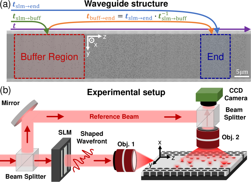
Figure 1: Waveguide structure and optical setup. A composite SEM image of a diffusive waveguide is shown in (a). The matrix mapping the field in the buffer region to the end region, $t_{\rm buff\rightarrow end}$, is related to the matrices $t_{\rm slm\rightarrow\rm buff}$ and $t_{\rm slm\rightarrow\rm end}$. In (b) the simplified sketch of the experimental setup illustrates how we wavefront shape a laser beam with a spatial light modulator (SLM) while performing an interferometric measurement of the light scattered out of the waveguide.

To directly observe the depth profiles of transmission eigenchannels within a diffusive system, we fabricate two-dimensional (2D) waveguide structures on a silicon-on-insulator wafer with electron beam lithography and plasma etching SM . As shown in Fig. 1(a), 100 nm-diameter holes are randomly etched into the waveguides, which have photonic crystal sidewalls to reflect light Yamilov et al. (2014). At the wavelength of our probe light, $\lambda=1.55$ µm, the transport mean free path, $\ell_{t}=3.2$ µm, is much shorter than the disordered region length, $L=50$ µm, in each waveguide. Therefore, the light undergoes multiple scattering and diffusive transport through each waveguide SM . Light scatters out-of-plane from the random holes, providing a direct probe of the light inside the disordered region. This process can be modeled as an effective loss, and accounted for in the diffusive dissipation length: $\xi_{a}$ = 28 µm. The waveguides are each 15 µm wide, supporting $N$ = 55 propagating modes at $\lambda=1.55$ µm. Before entering one of the diffusive waveguides, light is injected via the edge of the wafer into a ridge waveguide. Due to the large refractive index mismatch between silicon and air, only low-order waveguide modes are excited at the interface. Before the disordered region, the waveguide width is tapered from 300 µm to 15 µm in order to convert the lower-order modes to higher-order ones. The taper enables us to access all waveguide modes incident on the disordered region Sarma et al. (2016).

To measure the light field inside individual diffusive waveguides, we use an interferometric setup, as sketched in Fig. 1(b). In our setup, the monochromatic light from a wavelength-tunable laser source is split into two beams. One beam is modulated by a spatial light modulator (SLM) and then injected into one of the waveguides via the edge of the wafer. The other beam is used as a reference beam. It is spatially overlapped with the out-of-plane scattered light from the diffusive waveguide: on the CCD camera chip. The CCD camera records the resulting interference pattern, from which the complex field profile across the diffusive waveguide is obtained, as shown in SM .

By sequentially applying an orthogonal set of phase patterns to the 128 SLM macropixels, and measuring the field within the sample, we acquire a matrix that maps the field from the SLM to the field inside the disordered waveguide $t_{\rm slm\rightarrow\rm int}$. This matrix encompasses information about the light transport inside the waveguide and the light propagation from the SLM to the waveguide. To separate these, we need access to the field incident on the disordered region of the waveguide. We obtain this information by adding an auxiliary weakly-scattering region in front of the diffusive region called the ‘buffer’ region: as shown in Fig. 1 (a). From the light scattered out-of-plane from the buffer, we recover the field right in front of the strongly-scattering region. The length of the buffer region is 25 µm, which is shorter than its 32 µm-length transport mean free path. Therefore, light only experiences single scattering in the buffer, and as a result, the diffusive wave transport in the original disordered region is not appreciably altered.

With access to the field inside the buffer, we can construct the matrix relating the field on the SLM to the buffer, $t_{\rm slm\rightarrow\rm buff}$. From $t_{\rm slm\rightarrow\rm int}$, we can also construct the matrix, $t_{\rm slm\rightarrow\rm end}$, which maps the field from the SLM to a region near the end of the diffusive waveguide. With these we calculate the matrix which maps the field from the buffer to the end, $t_{\rm buff\rightarrow end}=t_{\rm slm\rightarrow end}\,t_{\rm slm\rightarrow buff}^{-1}$, using Moore-Penrose matrix inversion. Although $t_{\rm buff\rightarrow end}$ is not the field transmission matrix $t$, the depth profiles of its eigenchannels match those of transmission eigenchannels in our numerical simulation (see Fig. 2 and discussion below). Therefore, $t_{\rm buff\rightarrow end}$ can be used as an experimental proxy for the field transmission matrix, $t$, of the diffusive waveguide.

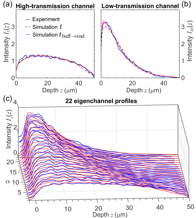
Figure 2: Depth profiles of transmission eigenchanels. High ($\alpha=1$) and low ($\alpha=20$) transmission eigenchannel profiles are presented in (a,b) while the 22 measured eigenchannel profiles are juxtaposed in (c). The experimentally measured profiles (blue lines) agree well with the profiles calculated from numerical simulations using the transmission matrix $t$ (black dashed lines) and the matrix $t_{\rm buff\rightarrow end}$ (red lines).

To excite a single eigenchannel, we first perform a singular value decomposition on $t_{\rm buff\rightarrow end}$ to obtain the field distribution in the buffer corresponding to one eigenchannel. Then we multiply the field profile in the buffer with $t^{-1}_{\rm slm\rightarrow buff}$ to calculate the SLM phase-modulation pattern. By displaying this pattern on the SLM, we excite a single eigenchannel of the diffusive waveguide. We record the spatial intensity profile of each eigenchannel within the diffusive waveguide. From this measurement, we obtain the eigenchannel depth profile $\tilde{I}(z)$ associated with each measurement by summing the intensity over the waveguide cross-section. For each depth profile, the measured intensity profile $\tilde{I}(z)$ is normalized to $I(z)=\tilde{I}(z)/[(1/L)\int_{0}^{L}\tilde{I}(z^{\prime})dz^{\prime}]$.

In Figures 2(a) and (b), the experimentally-measured depth profiles of a high-transmission and a low-transmission eigenchannel are juxtaposed. The high-transmission eigenchannel in (a) has an arch-shaped energy-density distribution which spans the depth of the diffusive region. In (b), the energy-density distribution of the low-transmission eigenchannel rapidly decays with depth. We numerically calculate the transmission eigenchannels with the recursive Green’s function method in the Kwant simulation package SM . The experimentally measured profiles match the corresponding depth profiles generated from numerical simulations of both $t$ and $t_{\rm buff\rightarrow end}$; confirming that we excite individual eigenchannels in our measurements. Furthermore, the agreement between the eigenchannels of $t_{\rm buff\rightarrow end}$ and $t$, confirms that the depth profiles of $t_{\rm buff\rightarrow end}$ have a one-to-one correspondence with the eigenchannels of $t$.

In total, we measure $50$ eigenchannel profiles for a single experimental system realization. Each profile matches one of the ensemble-averaged profiles of $t_{\rm buff\rightarrow end}$ generated numerically without any fitting parameters SM . Measurement noise causes multiple experimental profiles to be mapped to a single numerical profile, and this limits the total number of recovered eigenchannels to $22$. Fig. 2(c) shows the depth profiles for all $22$ eigenchannels, which agree well with the numerical simulations SM . The transmittance of the measured eigenchannels varies from $\tau_{1}\simeq 0.43$ to $\tau_{22}\simeq 7.9\times 10^{-4}$, with a mean value of $\langle\tau_{\alpha}\rangle=0.041$.

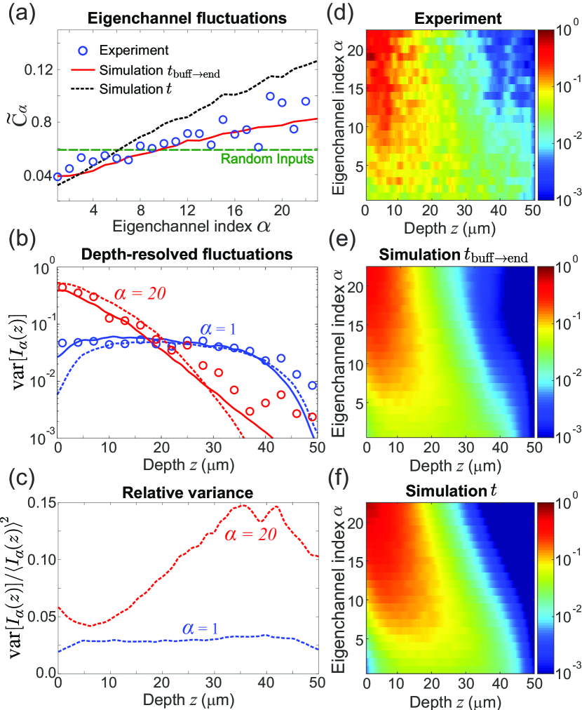
Figure 3: Eigenchannel fluctuations. In (a), the spatially-averaged depth-profile fluctuations of the eigenchannels, $\tilde{C}_{\alpha}$, increase monotonically with the channel index $\alpha$. The green dashed line indicates the experimentally observed fluctuations for random incident wavefronts: 0.59. In (b), experimentally observed depth-resolved intensity fluctuations, ${\rm var}[I_{\alpha}(z)]$, of high ($\alpha=1$) and low ($\alpha=20$) transmission eigenchannels (circles) are closely reproduced by the numerical simulations of transmission eigenchannels from $t_{\rm buff\rightarrow end}$ (solid lines) and $t$ (dashed lines). In (c), ${\rm var}[I_{\alpha}(z)]$ is divided by $\langle I_{\alpha}(z)\rangle^{2}$ for the high/low-transmission eigenchannels of $t$. In (d-e), the experimentally-observed and numerically-calculated depth-resolved intensity fluctuations for individual eigenchannels show how ${\rm var}[I_{\alpha}(z)]$ evolves with $\alpha$.

Next, we study the realization-to-realization fluctuations of eigenchannel profiles. From measurements of 13 system realizations SM , we compute the mean depth profile of each eigenchannel, $\langle I_{\alpha}(z)\rangle$, and the realization-specific deviation, $\delta I_{\alpha}(z)=I_{\alpha}(z)-\langle I_{\alpha}(z)\rangle$. From this, the total fluctuation of each eigenchannel profile is quantified by $\tilde{C}_{\alpha}=(1/L)\int_{0}^{L}\langle[\delta I_{\alpha}(z)]^{2}\rangle dz$, where $\langle...\rangle$ represents ensemble averaging. Fig. 3(a) shows that the total fluctuation of each eigenchannel profile increases monotonically as a function of eigenchannel index. The uncertainty of $\tilde{C}_{\alpha}$ -due to the finite number of ensembles in our experiment- is estimated from simulations to be $\pm 25\%$ the value of $\tilde{C}_{\alpha}$: which is smaller than the overall change of $\tilde{C}_{\alpha}$ with $\alpha$. Hence, the depth profiles of high-transmission eigenchannels fluctuate less than the profiles generated by random illumination patterns (indicated by the green dashed line); while lower-transmission eigenchannels fluctuate more.

Now we look into the position-dependent fluctuation of individual eigenchannel profiles about their ensemble average, ${\rm var}[I_{\alpha}(z)]=\langle[\delta I_{\alpha}(z)]^{2}\rangle$ as a function of depth, $z$. Fig. 3(b) reveals distinct differences in the depth dependence of high and low-transmission eigenchannels. While ${\rm var}[I_{\alpha}(z)]$ is nearly flat for the high-transmission eigenchannel, it features a fast drop with $z$ for the low-transmission eigenchannel. Figs. 3(d-f) are 2D plots of ${\rm var}[I_{\alpha}(z)]$ for all 22 eigenchannels: calculated using experimental data, as well as simulations of $t_{\rm buff\rightarrow end}$, and $t$. As the transmittance decreases, the maximum of ${\rm var}[I_{\alpha}(z)]$ moves towards the front surface of the diffusive region. The decrease in the variance with depth results from the decay of the mean intensity with depth: $\langle I_{\alpha}(z)\rangle$. However, the relative intensity fluctuation of the low-transmission eigenchannels, characterized by ${\rm var}[I_{\alpha}(z)]/\langle I_{\alpha}(z)\rangle^{2}$, actually increase with depth as shown in Fig. 3(c) for $\alpha=20$. In contrast, the relative intensity fluctuation of high-transmission eigenchannels is uniform with depth and small: for example ${\rm var}[I_{1}(z)]/\langle I_{1}(z)\rangle^{2}<0.04$ for all $z$. Moreover, the fluctuation of a transmission eigenchannel’s intensity at the sample output reflects the fluctuation of the corresponding transmission eigenvalue. Therefore, the stronger fluctuation of a low-transmission eigenchannel, relative to a high-transmission eigenchannel, at the output end $z=L$ indicates the fluctuation of its eigenvalue is similarly higher. This result, which we confirmed in our numerical simulations, is consistent with the theoretical prediction in Ref. Pichard et al. (1990).

The experimentally observed fluctuations of individual transmission eigenchannels are quantitatively reproduced by the numerical simulations of $t_{\rm buff\rightarrow end}$ and $t$ in Figs. 3(a,b,d-f). The excellent agreement between experimental and numerical results confirms that eigenchannel fluctuations depend on their transmittance. The higher the transmittance, the lower the fluctuations. This means that high-transmission eigenchannels have a robust and consistent depth profile: irrespective of the disorder configuration of a system.

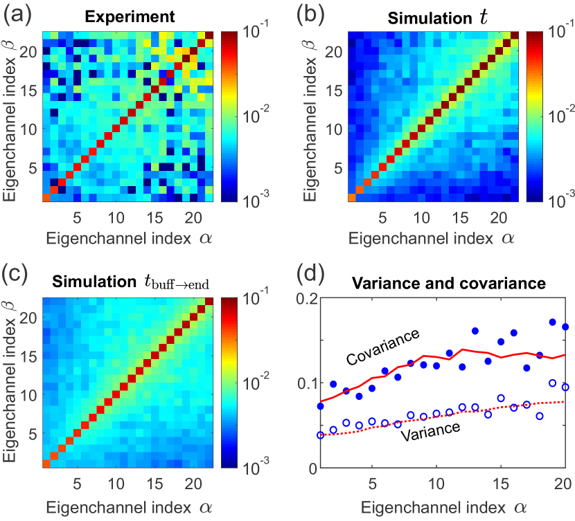
Figure 4: Inter-channel correlations. The covariance $\tilde{C}_{\alpha\beta}$ between any two pairs of eigenchannels, $\alpha$ and $\beta$, is calculated from experimental data (a) and numerical simulations (b,c). The cumulative covariance $\sum_{\beta\neq\alpha}\tilde{C}_{\alpha\beta}$ exceeds the variance $\tilde{C}_{\alpha\alpha}$ in (d). The blue symbols represent experimental data and red lines represent numerical simulations based on $t_{\rm buff\rightarrow end}$.

Finally, we investigate the cross-correlations between different transmission eigenchannels. For any given disorder realization, eigenchannels are an orthogonal set of functions at the front and back surfaces of the medium. While eigenchannels differ from realization-to-realization, their orthogonality implies that the differences in their field profiles must be correlated from realization-to-realization. This does not mean, however, that the intensity fluctuations of their profiles inside the sample should be correlated. To study cross-correlations in the eigenchannels’ intensity fluctuations across the sample, we introduce the covariance $\tilde{C}_{\alpha\beta}=\langle\delta I_{\alpha}(z)\delta I_{\beta}(z)\rangle_{z}$, where $\langle...\rangle_{z}$ describes both ensemble averaging and depth averaging. For $\alpha=\beta$, $\tilde{C}_{\alpha\alpha}$ reduces to the variance $\tilde{C}_{\alpha}$ which describes the eigenchannel fluctuations.

Fig. 4(a-c) shows the experimental and numerical results of $\tilde{C}_{\alpha\beta}$ for all $\alpha$ and $\beta$. The non-vanishing off-diagonal elements of $\tilde{C}_{\alpha\beta}$ ($\alpha\neq\beta$) reveal coordinated changes in the eigenchannels’ depth profiles. Between different pairings of eigenchannels, the correlations differ. The larger the difference in the transmittances of a pair, the weaker the correlation of their depth profile fluctuations. Furthermore, lower-transmission eigenchannels tend to correlate more with other low-transmission eigenchannels than higher-transmission eigenchannels do with other high-transmission eigenchannels. Quantitatively we can describe the correlation of a single eigenchannel to all others by the cumulative covariance $\sum_{\beta\neq\alpha}\tilde{C}_{\alpha\beta}$. As shown in Fig. 4(d), the cumulative covariance increases with $\alpha$, indicating higher-transmission eigenchannels are more independent from other eigenchannels than lower-transmission eigenchannels. Moreover, the cumulative covariance exceeds the variance $\tilde{C}_{\alpha\alpha}=\tilde{C}_{\alpha}$ by a factor of 2. Hence, the total cross-correlation for a single eigenchannel is stronger than its own fluctuation.

To provide a plausible explanation for the observed phenomena, we resort to the modal description of transmission eigenchannels Shi and Genack (2015). A transmission eigenchannel can be decomposed by the quasinormal modes of the disordered system. Previous research Shi and Genack (2015) has revealed that high-transmission eigenchannels are composed of only a few on-resonance modes, while low-transmission eigenchannels are composed of many off-resonance modes that destructively interfere. Since the destructive interference is sensitive to changes in the scattering configuration, the low-transmission eigenchannels exhibit strong fluctuations. Moreover, because individual low-transmission eigenchannels share many of the same off-resonant modes, their fluctuations are correlated. Since high-transmission eigenchannels are composed of a different set of modes than low-transmission eigenchannels, the correlations between high and low-transmission eigenchannels are weak.

Our findings regarding the second-order statistical properties of transmission eigenchannels are general and applicable to other types of waves such as microwaves, acoustic waves, and matter waves. In practical applications, the consistent and robust depth profiles of open channels guarantee that they can deliver energy deep into any diffusive system regardless of the disorder configuration. Such reliable energy delivery has major implications in applications ranging from multi-photon imaging to photothermal therapy, and shock wave treatment. Since our on-chip experimental platform allows for both direct measurement of the complex field inside a random structure and near-complete control over the incident field, we can investigate how to shape an incident wavefront to control the spatial distribution of light across the entire disordered sample. Furthermore, this setup can be used to experimentally study the spatial structure and statistics of the time-delay eigenchannels of a diffusive system, as well as the time-gated transmission and reflection eigenchannels of a diffusive system.