Bulk viscosity of resonating fermions revisited:
Kubo formula, sum rule, and the dimer and high-temperature limits

Abstract

The bulk viscosity of two-component fermions with a zero-range interaction is revisited both in two and three dimensions. We first point out that the “standard” Kubo formula employed in recent studies has flaws to give rise to an unphysical divergent bulk viscosity even in a limit where it is supposed to vanish. The corrected Kubo formula as well as the sum rule is then carefully rederived so as to confirm that the bulk viscosity indeed vanishes in the free, unitarity, and dimer limits. We also discuss that the recently found discrepancy between the Kubo formalism and the kinetic theory for the bulk viscosity is attributed to the fact that the quasiparticle approximation assumed by the latter breaks down even in the high-temperature limit.

I Introduction

Two-component fermions with a zero-range interaction constitute a system of simple elegance that is parametrized solely by a scattering length, $a$ Zwerger:2012 . As the inverse scattering length increases, the system evolves from a free Fermi gas (free limit) to a free Bose gas of tightly bound dimers (dimer limit). In particular, when the scattering length diverges (unitarity limit), the scale and conformal invariance emerge Mehen:2000 ; Son:2006 ; Nishida:2007 , so that its equation of state obeys the ideal gas law although the system is strongly interacting. The conformal invariance manifests itself also in dynamic properties such as the vanishing bulk viscosity Son:2007 ; Taylor:2010 ; Enss:2011 .

Recently, the frequency-dependent bulk viscosity (bulk viscosity spectral function) for an arbitrary scattering length was studied both in two and three dimensions based on the quantum virial expansion Nishida:2019 ; Enss:2019 ; Hofmann:2020 . The starting point was the “standard” Kubo formula for the bulk viscosity,

$$\operatorname{Re}[\zeta(\omega)]=\frac{\operatorname{Im}[R_{\Pi\Pi}(\omega)]}{\omega},$$ (1)

where

$$R_{XY}(\omega)=\frac{i}{L^{d}}\int_{0}^{\infty}\!dt\,e^{i(\omega+i0^{+})t}\langle[\hat{X}(t),\hat{Y}(0)]\rangle$$ (2)

for $\hat{X}=\hat{Y}=\hat{\Pi}$ is the stress-stress response function at zero wave vector. Because the trace of the integrated stress tensor operator is provided by $d\cdot\hat{\Pi}=2\hat{H}+\hat{C}/(\Omega_{d-1}ma^{d-2})$ and the commutator of the Hamiltonian with any operator in the grand canonical average vanishes, the above Kubo formula turns into the favorite form of

$$\operatorname{Re}[\zeta(\omega)]=\frac{1}{(d\cdot\Omega_{d-1}ma^{d-2})^{2}}\frac{\operatorname{Im}[R_{CC}(\omega)]}{\omega},$$ (3)

where $\hat{C}$ is the contact operator Martinez:2017 ; Fujii:2018 . It is its zero-frequency limit that corresponds to the bulk viscosity in hydrodynamics. The latter formula was then evaluated systematically in the high-temperature limit where the fugacity serves as a small expansion parameter Nishida:2019 ; Enss:2019 ; Hofmann:2020 .

Actually, these formulas have both technical and physical flaws (see also Ref. Bradlyn:2012 ). In order to derive Eq. (3), three terms such as $\operatorname{Im}[R_{HH}(\omega)]/\omega$ are dropped in Eq. (1) on the ground that the numerator vanishes. However, caution is required in the zero-frequency limit because the denominator also vanishes. Indeed, by employing the spectral representation,

$$R_{XY}(\omega) =-\frac{1}{L^{d}Z}\sum_{m,n}\frac{e^{-\beta E_{m}}-e^{-\beta E_{n}}}{\omega+E_{m}-E_{n}+i0^{+}}$$

$$\quad\times\langle m|\hat{X}|n\rangle\langle n|\hat{Y}|m\rangle,$$ (4)

and taking its imaginary part, one finds

$$\frac{\operatorname{Im}[R_{HH}(\omega)]}{\omega}=\frac{\pi}{L^{d}Z}\,\delta(\omega)\sum_{n}\beta e^{-\beta E_{n}}E_{n}^{2}$$ (5)

for $\hat{X}=\hat{Y}=\hat{H}$. This term thus diverges at zero frequency for an arbitrary scattering length including the free and unitarity limits where the bulk viscosity is supposed to vanish. Whether this and the other two terms should be dropped or not is ambiguous if one starts with Eq. (1).

Even if one takes Eq. (3) for granted, which now vanishes in the free and unitarity limits, it gives rise to a term proportional to $\delta(\omega)/a^{4}$ in the dimer limit (see Footnote 7 at the end of Sec. III.3). Because the system in the dimer limit is a free Bose gas of tightly bound dimers, it should exhibit scale invariance if probed at a lower frequency than their binding energy. Therefore, our physical intuition supposes that the bulk viscosity vanishes again, which conflicts with the divergent bulk viscosity of Eq. (3) in the dimer limit.

The purpose of this paper is to demonstrate that the above flaws are resolved by correcting the Kubo formula in Eq. (1). Although the corrected Kubo formula has been known since long ago Mori:1962 ; Luttinger:1964 , it is not well appreciated by the literature in the context of ultracold atom physics. Therefore, we first review its derivation as well as the sum rule in Sec. II and then carefully evaluate the corrected Kubo formula in Sec. III, confirming that the bulk viscosity indeed vanishes in the free, unitarity, and dimer limits. We also revisit the bulk viscosity in the high-temperature limit in Sec. IV and discuss a possible origin of the discrepancy between the Kubo formalism and the kinetic theory found recently in Refs. Nishida:2019 ; Enss:2019 ; Hofmann:2020 . Finally, Sec. V is devoted to a summary of this paper and some useful formulas regarding Kubo’s canonical correlation function are presented in Appendix A.

In what follows, we will set $\hbar=k_{B}=1$ and implicit summations over repeated indices are assumed throughout this paper. Also, an integration over $d$-dimensional wave vector or momentum is denoted by $\int_{\bm{k}}\equiv\int\!d{\bm{k}}/(2\pi)^{d}$ for the sake of brevity.

II Kubo formula

The Kubo formula for the bulk viscosity can be derived by matching current responses against an external force between microscopic and low-energy effective descriptions, the latter of which is of course hydrodynamics. Our derivation reviewed in this section partly follows that in Ref. Luttinger:1964 (see Appendix B therein).

II.1 Microscopics

We first consider that the system is weakly perturbed by an external vector potential, so that the microscopic Hamiltonian reads

$$\hat{H}\to\hat{H}^{A}(t)=\int\!d{\bm{r}}\,\frac{[D_{i}\hat{\psi}_{\sigma}({\bm{r}})]^{\dagger}[D_{i}\hat{\psi}_{\sigma}({\bm{r}})]}{2m}+\hat{V},$$ (6)

where $m$ is a mass of particles and $D_{i}\equiv\partial_{i}-iA_{i}(t,{\bm{r}})$ is the covariant derivative. Accordingly, the current density operator is modified into

$$\hat{\mathcal{J}}_{i}^{A}(t,{\bm{r}})\equiv-\frac{\delta\hat{H}^{A}(t)}{\delta A_{i}(t,{\bm{r}})}=\hat{\mathcal{J}}_{i}({\bm{r}})-\hat{\mathcal{N}}({\bm{r}})\frac{A_{i}(t,{\bm{r}})}{m}$$ (7)

with $\hat{\mathcal{N}}({\bm{r}})=\hat{\psi}_{\sigma}^{\dagger}({\bm{r}})\hat{\psi}_{\sigma}({\bm{r}})$ and $\hat{\mathcal{J}}_{i}({\bm{r}})=[\hat{\psi}_{\sigma}^{\dagger}({\bm{r}})\partial_{i}\hat{\psi}_{\sigma}({\bm{r}})-\partial_{i}\hat{\psi}_{\sigma}^{\dagger}({\bm{r}})\hat{\psi}_{\sigma}({\bm{r}})]/(2im)$ being the unperturbed number and current density operators, respectively. The linear-response theory predicts that the expectation value of Eq. (7) is provided by

$$\mathcal{J}_{i}(t,{\bm{r}}) =\langle\hat{\mathcal{J}}_{i}^{A}({\bm{r}})\rangle+i\int_{-\infty}^{t}\!dt^{\prime}\int\!d{\bm{r}}^{\prime}\langle[\hat{\mathcal{J}}_{i}(t,{\bm{r}}),\hat{\mathcal{J}}_{j}(t^{\prime},{\bm{r}}^{\prime})]\rangle$$

$$\quad\times A_{j}(t^{\prime},{\bm{r}}^{\prime})+O(A^{2}),$$ (8)

where $\hat{\mathcal{O}}(t,{\bm{r}})\equiv e^{i\hat{H}t}\hat{\mathcal{O}}({\bm{r}})e^{-i\hat{H}t}$ is an operator in the Heisenberg representation and $\langle\cdots\rangle\equiv\operatorname{Tr}[e^{-\beta(\hat{H}-\mu\hat{N})}\cdots]/\operatorname{Tr}[e^{-\beta(\hat{H}-\mu\hat{N})}]$ is an expectation value without the perturbation Altland-Simons . Then, by setting $\langle\hat{\mathcal{N}}({\bm{r}})\rangle=\mathcal{N}$ and $\langle\hat{\mathcal{J}}_{i}({\bm{r}})\rangle=0$ in thermodynamic equilibrium, the spacetime Fourier transformation leads to

$$\mathcal{J}_{i}(w,{\bm{k}})=-\mathcal{N}\frac{A_{i}(w,{\bm{k}})}{m}+R_{\mathcal{J}_{i}\mathcal{J}_{j}}(w,{\bm{k}})A_{j}(w,{\bm{k}})+O(A^{2}),$$ (9)

where

$$R_{\mathcal{X}\mathcal{Y}}(w,{\bm{k}})\equiv i\int_{0}^{\infty}\!dt\int\!d{\bm{r}}\,e^{iwt-i{\bm{k}}\cdot{\bm{r}}}\langle[\hat{\mathcal{X}}(t,{\bm{r}}),\hat{\mathcal{Y}}(0,{\bm{0}})]\rangle$$ (10)

is a response function and $w$ denotes an arbitrary complex frequency with $\operatorname{Im}[w]>0$. Although $w$ is eventually replaced by $\omega+i0^{+}$ for a real frequency $\omega$, it is of technical help to work on the upper-half plane of complex $w$ until the very end of all calculations.

It will turn out to be favorable to express the current-current response function in terms of Kubo’s canonical correlation function,

$$K_{\mathcal{X}\mathcal{Y}}(w,{\bm{k}}) \equiv\int_{0}^{\infty}\!dt\int\!d{\bm{r}}\,e^{iwt-i{\bm{k}}\cdot{\bm{r}}}\int_{0}^{\beta}\!\frac{d\tau}{\beta}$$

$$\quad\times\langle\delta\hat{\mathcal{X}}(t-i\tau,{\bm{r}})\delta\hat{\mathcal{Y}}(0,{\bm{0}})\rangle,$$ (11)

where $\delta\hat{\mathcal{O}}(t,{\bm{r}})\equiv\hat{\mathcal{O}}(t,{\bm{r}})-\langle\hat{\mathcal{O}}(t,{\bm{r}})\rangle$ is an operator with its expectation value subtracted Kubo:1957 . After some calculations as detailed in Appendix A.1, we obtain

$$iwR_{\mathcal{J}_{i}\mathcal{J}_{j}}(w,{\bm{k}})=-\beta K_{\pi_{ik}\pi_{jl}}(w,{\bm{k}})\frac{k_{k}k_{l}}{m^{2}},$$ (12)

where $\hat{\pi}_{ij}({\bm{r}})$ is the unperturbed stress tensor operator obeying the momentum continuity equation,

$$m\partial_{t}\hat{\mathcal{J}}_{i}(t,{\bm{r}})+\partial_{j}\hat{\pi}_{ij}(t,{\bm{r}})=0.$$ (13)

Therefore, the current response is found to be

$$\mathcal{J}_{i}(w,{\bm{k}}) =-\left[m\mathcal{N}\delta_{ij}+\beta K_{\pi_{ik}\pi_{jl}}(w,{\bm{k}})\frac{k_{k}k_{l}}{iw}\right]\frac{A_{j}(w,{\bm{k}})}{m^{2}}$$

$$\quad+O(A^{2})$$ (14)

in the microscopic description.

II.2 Hydrodynamics

We then consider that the system perturbed at low frequency and wave vector is described by hydrodynamics, which is founded on the number continuity equation,

$$\partial_{t}\mathcal{N}(t,{\bm{r}})+\partial_{i}\mathcal{J}_{i}(t,{\bm{r}})=0,$$ (15)

the momentum continuity equation,

$$m\partial_{t}\mathcal{J}_{i}(t,{\bm{r}})+\partial_{j}\pi_{ij}(t,{\bm{r}})$$

$$=\mathcal{N}(t,{\bm{r}})E_{i}(t,{\bm{r}})+\mathcal{J}_{j}(t,{\bm{r}})F_{ij}(t,{\bm{r}}),$$ (16)

and the energy continuity equation,

$$\partial_{t}\mathcal{H}(t,{\bm{r}})+\partial_{i}\mathcal{Q}_{i}(t,{\bm{r}})=\mathcal{J}_{i}(t,{\bm{r}})E_{i}(t,{\bm{r}}).$$ (17)

Here, $E_{i}(t,{\bm{r}})=-\partial_{t}A_{i}(t,{\bm{r}})$ and $F_{ij}=\partial_{i}A_{j}(t,{\bm{r}})-\partial_{j}A_{i}(t,{\bm{r}})$ are the external electric and magnetic fields, respectively, and the conserved charge densities and their fluxes are to be expressed in terms of the local thermodynamic variables and the fluid flow velocity $v_{i}(t,{\bm{r}})$. The constitutive relations for normal fluids read

$$\mathcal{J}_{i}(t,{\bm{r}})=\mathcal{N}(t,{\bm{r}})v_{i}(t,{\bm{r}})$$ (18)

for the number current density,

$$\mathcal{H}(t,{\bm{r}})=\mathcal{E}(t,{\bm{r}})+\frac{m}{2}\mathcal{N}(t,{\bm{r}})[{\bm{v}}(t,{\bm{r}})]^{2}$$ (19)

for the energy density,

$$\pi_{ij}(t,{\bm{r}}) =p(t,{\bm{r}})\delta_{ij}+m\mathcal{N}(t,{\bm{r}})v_{i}(t,{\bm{r}})v_{j}(t,{\bm{r}})$$

$$\quad-\sigma_{ij}(t,{\bm{r}})$$ (20)

for the stress tensor,

$$\mathcal{Q}_{i}(t,{\bm{r}}) =[\mathcal{H}(t,{\bm{r}})+p(t,{\bm{r}})]v_{i}(t,{\bm{r}})$$

$$\quad-\sigma_{ij}(t,{\bm{r}})v_{j}(t,{\bm{r}})-\kappa\,\partial_{i}T(t,{\bm{r}})$$ (21)

for the energy current density with

$$\sigma_{ij} =\left(\zeta-\frac{2}{d}\,\eta\right)\delta_{ij}\partial_{k}v_{k}(t,{\bm{r}})$$

$$\quad+\eta\,[\partial_{i}v_{j}(t,{\bm{r}})+\partial_{j}v_{i}(t,{\bm{r}})],$$ (22)

where $\zeta$ is the bulk viscosity, $\eta$ is the shear viscosity, and $\kappa$ is the thermal conductivity Landau-Lifshitz . We choose the number density $\mathcal{N}(t,{\bm{r}})$ and the internal energy density $\mathcal{E}(t,{\bm{r}})$ as the independent variables, so that the pressure $p(t,{\bm{r}})=p[\mathcal{N}(t,{\bm{r}}),\mathcal{E}(t,{\bm{r}})]$ and the temperature $T(t,{\bm{r}})=T[\mathcal{N}(t,{\bm{r}}),\mathcal{E}(t,{\bm{r}})]$ are locally determined by the equations of state.

When the perturbation by the external vector potential is weak, the thermodynamic variables slightly deviate from their equilibrium values, so that $\delta\mathcal{N}(t,{\bm{r}})=\mathcal{N}(t,{\bm{r}})-\mathcal{N}$, $\delta\mathcal{E}(t,{\bm{r}})=\mathcal{E}(t,{\bm{r}})-\mathcal{E}$, and $v_{i}(t,{\bm{r}})$ are as small as $O(A)$. After linearizing the hydrodynamic equations in Eqs. (15)–(17), the spacetime Fourier transformation leads to

$$-iw\delta\mathcal{N}(w,{\bm{k}})+\mathcal{N}ik_{i}v_{i}(w,{\bm{k}})=0,$$ (23)

$$-m\mathcal{N}iwv_{i}(w,{\bm{k}})+\left(\frac{\partial p}{\partial\mathcal{N}}\right)_{\mathcal{E}}ik_{i}\delta\mathcal{N}(w,{\bm{k}})$$

$$\quad+\left(\frac{\partial p}{\partial\mathcal{E}}\right)_{\mathcal{N}}ik_{i}\delta\mathcal{E}(w,{\bm{k}})+\left(\zeta+\frac{d-2}{d}\eta\right)k_{i}k_{j}v_{j}(w,{\bm{k}})$$

$$\quad+\eta\,{\bm{k}}^{2}v_{i}(w,{\bm{k}})=\mathcal{N}iwA_{i}(w,{\bm{k}}),$$ (24)

$$-iw\delta\mathcal{E}(w,{\bm{k}})+(\mathcal{E}+p)ik_{i}v_{i}(w,{\bm{k}})$$

$$\quad+\kappa\left(\frac{\partial T}{\partial\mathcal{N}}\right)_{\mathcal{E}}{\bm{k}}^{2}\delta\mathcal{N}(w,{\bm{k}})+\kappa\left(\frac{\partial T}{\partial\mathcal{E}}\right)_{\mathcal{N}}{\bm{k}}^{2}\delta\mathcal{E}(w,{\bm{k}})=0.$$ (25)

Finally, by eliminating $\delta\mathcal{N}(w,{\bm{k}})$ and $\delta\mathcal{E}(w,{\bm{k}})$, the current response up to $O(k^{2})$ is found to be

$$\mathcal{J}_{i}(w,{\bm{k}})=-\,\biggl{[}m\mathcal{N}\delta_{ij}-\left(\frac{\partial p}{\partial\mathcal{N}}\right)_{\mathcal{E}}\mathcal{N}\frac{k_{i}k_{j}}{(iw)^{2}}$$

$$\quad-\left(\frac{\partial p}{\partial\mathcal{E}}\right)_{\mathcal{N}}(\mathcal{E}+p)\frac{k_{i}k_{j}}{(iw)^{2}}+\left(\zeta+\frac{d-2}{d}\eta\right)\frac{k_{i}k_{j}}{iw}$$

$$\quad+\eta\,\frac{{\bm{k}}^{2}}{iw}\delta_{ij}+O(k^{3})\biggr{]}\,\frac{A_{j}(w,{\bm{k}})}{m^{2}}+O(A^{2})$$ (26)

in the hydrodynamic description.

Here, it is worthwhile to emphasize that the second and third terms in the square brackets of Eq. (II.2) originate from the pressure fluctuations associated with the fluctuations of the number and energy densities, respectively, which are essential to the correct Kubo formula for the bulk viscosity Mori:1962 . However, such pressure fluctuations were neglected in Ref. Taylor:2010 by stating “In the long-wavelength limit, the contributions to the stress tensor coming from viscous terms dominate over contributions from pressure fluctuations,” which we find ungrounded because both the contributions are $O(k^{2})$. We also note that the second and third terms are combined into the sound velocity,

$$mc_{s}^{2}\equiv\left(\frac{\partial p}{\partial\mathcal{N}}\right)_{\mathcal{S}/\mathcal{N}}=\left(\frac{\partial p}{\partial\mathcal{N}}\right)_{\mathcal{E}}+\left(\frac{\partial p}{\partial\mathcal{E}}\right)_{\mathcal{N}}\frac{\mathcal{E}+p}{\mathcal{N}},$$ (27)

so as to relate the pressure fluctuations to the gapless sound mode with $\mathcal{S}$ being the entropy density.

II.3 Bulk viscosity

Now, by matching the current responses between the microscopic and hydrodynamic descriptions in Eqs. (II.1) and (II.2) at low frequency and wave vector, we obtain

$$\lim_{w\to i0^{+}}\left[\beta K_{\pi_{ik}\pi_{jl}}(w,{\bm{0}})\frac{k_{k}k_{l}}{{\bm{k}}^{2}}+\frac{mc_{s}^{2}\mathcal{N}}{iw}\frac{k_{i}k_{j}}{{\bm{k}}^{2}}\right]$$

$$=\left(\zeta+\frac{d-2}{d}\eta\right)\frac{k_{i}k_{j}}{{\bm{k}}^{2}}+\eta\,\delta_{ij}.$$ (28)

Here, $K_{\pi_{ik}\pi_{jl}}(w,{\bm{0}})$ is symmetric under the exchanges of $i\leftrightarrow k$ and $j\leftrightarrow l$ by definition of the stress tensor operator as well as under $(ik)\leftrightarrow(jl)$ according to the Onsager reciprocal relations. Because the rotational invariance dictates that such a fourth-order tensor is decomposed into a sum of $\delta_{ik}\delta_{jl}$ and $\delta_{ij}\delta_{kl}+\delta_{il}\delta_{jk}$, we find

$$\lim_{w\to i0^{+}}\left[\beta K_{\pi_{ik}\pi_{jl}}(w,{\bm{0}})+\frac{mc_{s}^{2}\mathcal{N}}{iw}\delta_{ik}\delta_{jl}\right]$$

$$=\left(\zeta-\frac{2}{d}\,\eta\right)\delta_{ik}\delta_{jl}+\eta\,(\delta_{ij}\delta_{kl}+\delta_{il}\delta_{jk}),$$ (29)

so that the bulk and shear viscosities are provided by

$$\zeta =\lim_{w\to i0^{+}}\left[\beta K_{\pi\pi}(w,{\bm{0}})+\frac{mc_{s}^{2}\mathcal{N}}{iw}\right],$$ (30)

$$\eta =\lim_{w\to i0^{+}}\beta K_{\pi_{xy}\pi_{xy}}(w,{\bm{0}}),$$ (31)

where $d\cdot\hat{\pi}({\bm{r}})\equiv\hat{\pi}_{ii}({\bm{r}})$ is the trace of the stress tensor operator.

It is customary to refer to the right-hand side of Eq. (30),

$$\zeta(w)\equiv\beta K_{\pi\pi}(w,{\bm{0}})+\frac{mc_{s}^{2}\mathcal{N}}{iw},$$ (32)

as a frequency-dependent complex bulk viscosity for $w\to\omega+i0^{+}$. Because the bulk viscosity is provided by $\zeta=\lim_{w\to i0^{+}}\zeta(w)$, the singularity of the second term at $w=0$ originating from the gapless sound mode should be canceled by the same singularity inherent in the first term. Actually, the two terms can elegantly be combined so as to modify the stress tensor operator as

$$\hat{\tilde{\pi}}({\bm{r}})\equiv\hat{\pi}({\bm{r}})-\left[\left(\frac{\partial p}{\partial\mathcal{N}}\right)_{\mathcal{E}}\hat{\mathcal{N}}({\bm{r}})+\left(\frac{\partial p}{\partial\mathcal{E}}\right)_{\mathcal{N}}\hat{\mathcal{H}}({\bm{r}})\right],$$ (33)

where the subtracted terms represent the pressure fluctuations with $\hat{\mathcal{N}}({\bm{r}})$ and $\hat{\mathcal{H}}({\bm{r}})$ being the number and energy density operators, respectively. After some calculations as detailed in Appendix A.2, we obtain the succinct form of

$$\zeta(w)=\beta K_{\tilde{\pi}\tilde{\pi}}(w,{\bm{0}}),$$ (34)

which is nothing other than the Kubo formula for the bulk viscosity Mori:1962 ; Luttinger:1964 . We note that the canonical correlation function is favorable to clean up the rather involved expression in terms of the stress-stress response function Bradlyn:2012 , as detailed in Appendix A.3.

II.4 Sum rule

The sum rule for the frequency-dependent complex bulk viscosity from Eq. (32) reads

$$\int_{-\infty}^{\infty}\!\frac{d\omega}{\pi}\,\zeta(\omega+i0^{+})$$

$$=\int\!d{\bm{r}}\int_{0}^{\beta}\!d\tau\,\langle\delta\hat{\pi}(-i\tau,{\bm{r}})\delta\hat{\pi}(0,{\bm{0}})\rangle-mc_{s}^{2}\mathcal{N},$$ (35)

where the frequency integration sets the two operators at equal time. In order to further evaluate it, we from now on specialize to two-component fermions with a zero-range interaction in $d$ spatial dimensions, for which the trace of the stress tensor operator is provided by

$$\hat{\pi}({\bm{r}})=\frac{2\hat{\mathcal{H}}({\bm{r}})}{d}+\frac{\hat{\mathcal{C}}({\bm{r}})}{d\cdot\Omega_{d-1}ma^{d-2}}$$ (36)

up to irrelevant total derivatives Fujii:2018 . Here, $\Omega_{d-1}\equiv(4\pi)^{d/2}/2\Gamma(2-d/2)=2,\,2\pi,\,4\pi$ coincides with the surface area of the unit $(d-1)$-sphere for $d=1,\,2,\,3$ and $\hat{\mathcal{C}}({\bm{r}})$ is the contact density operator Braaten:2008 , which is related to the derivative of the Hamiltonian density with respect to the scattering length as

$$\hat{\mathcal{C}}({\bm{r}})=\Omega_{d-1}ma^{d-1}\frac{\partial\hat{\mathcal{H}}({\bm{r}})}{\partial a}.$$ (37)

Accordingly, the derivative of the stress tensor operator with respect to the scattering length turns into

$$\frac{\partial\hat{\pi}({\bm{r}})}{\partial a}=\frac{(4-d)\,\hat{\mathcal{C}}({\bm{r}})}{d\cdot\Omega_{d-1}ma^{d-1}},$$ (38)

because of $\partial\hat{\mathcal{C}}({\bm{r}})/\partial a=0$ for $2\leq d<4$. The spatial integrals of $\hat{\mathcal{N}}({\bm{r}})$, $\hat{\mathcal{H}}({\bm{r}})$, $\hat{\mathcal{C}}({\bm{r}})$, and $\hat{\pi}({\bm{r}})$ are to be denoted by $\hat{N}$, $\hat{H}$, $\hat{C}$, and $\hat{\Pi}$, respectively, and their expectation values by $\mathcal{O}=\langle\hat{\mathcal{O}}({\bm{r}})\rangle$ except for the pressure $p=\langle\hat{\pi}({\bm{r}})\rangle$.

Then, by employing the following properties of the canonical correlation function at equal time,

$$\int_{0}^{\beta}\!d\tau\,\langle\delta\hat{H}(-i\tau)\delta\hat{\mathcal{O}}({\bm{0}})\rangle=-\beta\left(\frac{\partial\langle\hat{\mathcal{O}}({\bm{0}})\rangle}{\partial\beta}\right)_{\beta\mu,a},$$ (39)

$$\int_{0}^{\beta}\!d\tau\,\langle\delta\hat{C}(-i\tau)\delta\hat{\mathcal{O}}({\bm{0}})\rangle$$

$$=-\Omega_{d-1}ma^{d-1}\left[\left(\frac{\partial\langle\hat{\mathcal{O}}({\bm{0}})\rangle}{\partial a}\right)_{\beta,\mu}-\left\langle\frac{\partial\hat{\mathcal{O}}({\bm{0}})}{\partial a}\right\rangle\right],$$ (40)

as well as the thermodynamic identities,

$$\left(\frac{\partial p}{\partial\beta}\right)_{\beta\mu,a} =-\frac{\mathcal{E}+p}{\beta},$$ (41)

$$\left(\frac{\partial p}{\partial a}\right)_{\beta,\mu} =-\frac{\mathcal{C}}{\Omega_{d-1}ma^{d-1}},$$ (42)

the sum rule for the frequency-dependent complex bulk viscosity is found to be

$$\int_{-\infty}^{\infty}\!\frac{d\omega}{\pi}\,\zeta(\omega+i0^{+})=\frac{d+2}{d}p+\frac{(4-d)\,\mathcal{C}}{d^{2}\cdot\Omega_{d-1}ma^{d-2}}-mc_{s}^{2}\mathcal{N}.$$ (43)

Our sum rule determined solely by thermodynamics turns out to coincide with that derived in Ref. Taylor:2010 , which we find unexpected because the last term originates from the pressure fluctuations neglected therein. Finally, the thermodynamic identities together with the dimensional analysis, as detailed in Appendix E of Ref. Taylor:2010 , simplifies the sum rule into

$$\int_{-\infty}^{\infty}\!\frac{d\omega}{\pi}\,\zeta(\omega+i0^{+})=-\frac{a^{3-d}}{d^{2}\cdot\Omega_{d-1}m}\left(\frac{\partial\mathcal{C}}{\partial a}\right)_{\mathcal{N},\mathcal{S}}.$$ (44)

Here, both $\mathcal{N}$ and $\mathcal{S}$ (as opposed to $\mathcal{S}/\mathcal{N}$ Taylor:2010 ; Taylor:2012 ) should be fixed in differentiating $\mathcal{C}$ with respect to $a$.

III Free, unitarity, and dimer limits

We evaluate the Kubo formula for the frequently-dependent complex bulk viscosity derived in the previous section, whose real part is supposed to vanish at an arbitrary frequency in the free and unitarity limits and at a lower frequency than the binding energy of dimers in the dimer limit.

III.1 Free and unitarity limits

In the free and unitarity limits where the system is scale invariant, the last term of the stress tensor operator in Eq. (36) is negligible because $\hat{\mathcal{C}}({\bm{r}})$ vanishes in the free limit and $a$ diverges in the unitarity limit. Accordingly, the equation of state obeys the ideal gas law, $p=2\mathcal{E}/d$, so that the modified stress tensor operator in Eq. (33) reads $\hat{\tilde{\pi}}({\bm{r}})=0$. Therefore, the frequency-dependent complex bulk viscosity is found to vanish at an arbitrary frequency,

$$\zeta(\omega+i0^{+})=0,$$ (45)

without any ambiguity discussed in Sec. I because the operator evaluated by the Kubo formula in Eq. (34) is identically zero.

III.2 Contact correlation

Although the canonical correlation function provides the succinct form of the frequently-dependent complex bulk viscosity, the response function is of practical help because the standard diagrammatic method can be applied. As detailed in Appendix A.3, Eq. (32) can be expressed in terms of the stress-stress response function and the sum rule as

$$\zeta(w)=\frac{R_{\pi\pi}(w,{\bm{0}})}{iw}-\frac{1}{iw}\int_{-\infty}^{\infty}\!\frac{d\omega}{\pi}\,\zeta(\omega+i0^{+}).$$ (46)

In particular, for two-component fermions with a zero-range interaction, the substitution of Eqs. (36) and (44) leads to

$$\zeta(w)=\frac{1}{iw}\frac{R_{\mathcal{C}\mathcal{C}}(w,{\bm{0}})}{(d\cdot\Omega_{d-1}ma^{d-2})^{2}}+\frac{1}{iw}\frac{a^{3-d}}{d^{2}\cdot\Omega_{d-1}m}\left(\frac{\partial\mathcal{C}}{\partial a}\right)_{\mathcal{N},\mathcal{S}},$$ (47)

where the commutator of the Hamiltonian with any operator in the grand canonical average can safely be dropped by working on the upper-half plane of complex $w$.

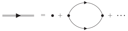
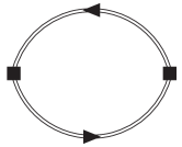
Figure 1: Diagrammatic representation of (top) the pair propagator and (bottom) the contact-contact response function, which become exact both in the dimer limit and in the high-temperature limit. The single and double lines represent the fermion and pair propagators, respectively, whereas the dot is a bare coupling constant and the square is to insert the contact density operator.

In order to evaluate the contact-contact response function, we first introduce the pair propagator in the medium above the superfluid critical temperature Melo:1993 ,

$$[D(ip_{0},{\bm{p}})]^{-1}=\frac{1}{g}-\int_{\bm{q}}\,\frac{1-f_{F}\!\left(\frac{({\bm{p}}/2+{\bm{q}})^{2}}{2m}\right)-f_{F}\!\left(\frac{({\bm{p}}/2-{\bm{q}})^{2}}{2m}\right)}{ip_{0}-\frac{{\bm{p}}^{2}}{4m}-\frac{{\bm{q}}^{2}}{m}+2\mu},$$ (48)

whose diagrammatic representation is depicted in Fig. 1. Here, $g<0$ is a bare coupling constant, $p_{0}=2\pi n/\beta$ is the bosonic Matsubara frequency, and $f_{F}(\varepsilon)=1/[e^{\beta(\varepsilon-\mu)}+1]$ is the Fermi-Dirac distribution function. Figure 1 also depicts the diagrammatic representation of the contact-contact response function,

$$R_{\mathcal{C}\mathcal{C}}(ik_{0},{\bm{k}})=\frac{m^{4}}{\beta}\sum_{p_{0}}\int_{\bm{p}}\,D(ik_{0}+ip_{0},{\bm{k}}+{\bm{p}})D(ip_{0},{\bm{p}}),$$ (49)

which fully incorporates two-body physics and thus becomes exact both in the dimer limit and in the high-temperature limit. The summation over the bosonic Matsubara frequency can be performed by employing the complex contour integration together with the spectral representation of the pair propagator,

$$D(ip_{0},{\bm{p}})=\int_{-\infty}^{\infty}\!\frac{dE}{\pi}\,\frac{\operatorname{Im}[D(E-i0^{+},{\bm{p}})]}{ip_{0}-E},$$ (50)

so that we obtain

$$R_{\mathcal{C}\mathcal{C}}(ik_{0},{\bm{k}})=-\iint_{-\infty}^{\infty}\!\frac{dE}{\pi}\frac{dE^{\prime}}{\pi}\int_{\bm{p}}\,\left(\frac{1}{e^{\beta E}-1}-\frac{1}{e^{\beta E^{\prime}}-1}\right)$$

$$\quad\times\frac{\operatorname{Im}[m^{2}D(E-i0^{+},{\bm{k}}+{\bm{p}})]\operatorname{Im}[m^{2}D(E^{\prime}-i0^{+},{\bm{p}})]}{ik_{0}+E-E^{\prime}}.$$ (51)

Finally, by setting $ik_{0}\to w$ and ${\bm{k}}={\bm{0}}$ and changing the integration variables to $\varepsilon^{(\prime)}=E^{(\prime)}-\frac{{\bm{p}}^{2}}{4m}+2\mu$, the contact-contact response function turns into

$$R_{\mathcal{C}\mathcal{C}}(w,{\bm{0}})$$

$$=-\iint_{-\infty}^{\infty}\!\frac{d\varepsilon}{\pi}\frac{d\varepsilon^{\prime}}{\pi}\int_{\bm{p}}\,\left[f_{B}\!\left(\varepsilon+\tfrac{{\bm{p}}^{2}}{4m}\right)-f_{B}\!\left(\varepsilon^{\prime}+\tfrac{{\bm{p}}^{2}}{4m}\right)\right]$$

$$\quad\times\frac{\operatorname{Im}[m^{2}D_{\bm{p}}(\varepsilon-i0^{+})]\operatorname{Im}[m^{2}D_{\bm{p}}(\varepsilon^{\prime}-i0^{+})]}{w+\varepsilon-\varepsilon^{\prime}},$$ (52)

where $f_{B}(\varepsilon)=1/[e^{\beta(\varepsilon-2\mu)}-1]$ is the Bose-Einstein distribution function and $D_{\bm{p}}(\varepsilon)\equiv D(\varepsilon+{\bm{p}}^{2}/4m-2\mu,{\bm{p}})$ is the pair propagator in the center-of-mass frame with the residual dependence on its momentum due to the medium.

Similarly, the contact density itself is provided by

$$\mathcal{C}=-\frac{m^{2}}{\beta}\sum_{p_{0}}\int_{\bm{p}}\,e^{ip_{0}0^{+}}D(ip_{0},{\bm{p}}),$$ (53)

where the summation over the bosonic Matsubara frequency leads to

$$\mathcal{C}=\int_{-\infty}^{\infty}\!\frac{d\varepsilon}{\pi}\int_{\bm{p}}\,f_{B}\!\left(\varepsilon+\tfrac{{\bm{p}}^{2}}{4m}\right)\operatorname{Im}[m^{2}D_{\bm{p}}(\varepsilon-i0^{+})]$$ (54)

with the same pair propagator introduced above.

III.3 Dimer limit

The pair propagator is further simplified in the dimer limit, $a\to+0$, where $f_{F}(\varepsilon>0)$ and $f_{B}(\varepsilon>0)$ are negligible because of $2\mu=-1/ma^{2}\to-\infty$, so that the pair propagator is reduced to that in the vacuum. The integration over ${\bm{q}}$ can thus be performed to lead to

$$D(\varepsilon-i0^{+})=\frac{\Omega_{d-1}}{m}\frac{d-2}{a^{2-d}-(-m\varepsilon+i0^{+})^{d/2-1}},$$ (55)

where the subscript of ${\bm{p}}$ is dropped on the left-hand side and the bare coupling constant is replaced by

$$g=\frac{\Omega_{d-1}}{m}\frac{d-2}{a^{2-d}-\frac{\Lambda^{d-2}}{\Gamma(d/2)\Gamma(2-d/2)}}$$ (56)

in the cutoff regularization with $|{\bm{q}}|<\Lambda$. By substituting its imaginary part,

$$\operatorname{Im}[D(\varepsilon-i0^{+})] =\theta(a)\,\frac{2\pi\Omega_{d-1}}{m^{2}a^{4-d}}\,\delta\!\left(\varepsilon+\tfrac{1}{ma^{2}}\right)$$

$$\quad+\theta(\varepsilon)\operatorname{Im}[D(\varepsilon-i0^{+})],$$ (57)

into the contact-contact response function in Eq. (III.2), we obtain

$$R_{\mathcal{C}\mathcal{C}}(w,{\bm{0}}) =\frac{\Omega_{d-1}m^{2}\mathcal{N}}{a^{4-d}}\int_{0}^{\infty}\!\frac{d\varepsilon}{\pi}\operatorname{Im}[D(\varepsilon-i0^{+})]$$

$$\quad\times\left(\frac{1}{\varepsilon+\frac{1}{ma^{2}}-w}+\frac{1}{\varepsilon+\frac{1}{ma^{2}}+w}\right),$$ (58)

where $\mathcal{N}=2\int_{\bm{p}}f_{B}({\bm{p}}^{2}/4m-1/ma^{2})$ is the number density with $1/ma^{2}$ being the binding energy of dimers.

Now, turning to thermodynamics in the dimer limit, the pressure of a free Bose gas of tightly bound dimers is provided by

$$p=-\frac{1}{\beta}\int_{\bm{p}}\,\ln\!\left\{1-\exp\!\left[-\beta\left(\tfrac{{\bm{p}}^{2}}{4m}-\tfrac{1}{ma^{2}}-2\mu\right)\right]\right\},$$ (59)

from which all thermodynamic variables are readily obtained including

$$\left(\frac{\partial\mathcal{C}}{\partial a}\right)_{\mathcal{N},\mathcal{S}}=-\frac{\Omega_{d-1}(4-d)\mathcal{N}}{a^{5-d}}.$$ (60)

Then, by employing the following identity,

$$\frac{\Omega_{d-1}(4-d)}{2ma^{2-d}}=\int_{0}^{\infty}\!\frac{d\varepsilon}{\pi}\,\frac{\operatorname{Im}[D(\varepsilon-i0^{+})]}{\varepsilon+\frac{1}{ma^{2}}},$$ (61)

and comparing it with Eq. (III.3), the sum rule is found to be related to the contact-contact response function at $w=0$ as

$$-\frac{a^{3-d}}{d^{2}\cdot\Omega_{d-1}m}\left(\frac{\partial\mathcal{C}}{\partial a}\right)_{\mathcal{N},\mathcal{S}}=\frac{R_{\mathcal{C}\mathcal{C}}(0,{\bm{0}})}{(d\cdot\Omega_{d-1}ma^{d-2})^{2}}.$$ (62)

Accordingly, the substitution of Eqs. (III.3) and (62) into Eq. (47) leads to

$$\zeta(w) =\frac{\mathcal{N}}{d^{2}\cdot\Omega_{d-1}a^{d}}\int_{0}^{\infty}\!\frac{d\varepsilon}{i\pi}\,\frac{\operatorname{Im}[D(\varepsilon-i0^{+})]}{\varepsilon+\frac{1}{ma^{2}}}$$

$$\quad\times\left(\frac{1}{\varepsilon+\frac{1}{ma^{2}}-w}-\frac{1}{\varepsilon+\frac{1}{ma^{2}}+w}\right).$$ (63)

The resulting frequency-dependent complex bulk viscosity is plotted in Fig. 2 for $w\to\omega+i0^{+}$, which is exact in the limit of $a\to+0$ at fixed temperature and number density. In particular, we find that its real part indeed vanishes at a lower frequency than the binding energy of dimers without the unphysical divergence at zero frequency, whereas the bound-continuum transition turns possible above the dimer-breakup threshold. We also note that our $\operatorname{Re}[\zeta(\omega+i0^{+})]$ in the dimer limit for $d=2$ coincides with the zero-temperature and zero-density limit of the bulk viscosity spectral function in Ref. Taylor:2012 .

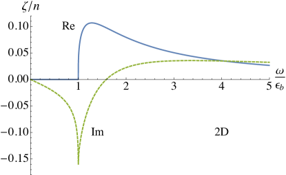
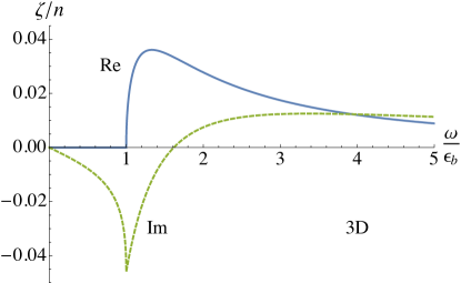
Figure 2: Frequency-dependent complex bulk viscosity $\zeta(\omega+i0^{+})$ in the dimer limit for (top) $d=2$ and (bottom) $d=3$ in units of the number density. Its real and imaginary parts are plotted by the solid and dashed curves, respectively, and the frequency is normalized by the binding energy of dimers.

IV High-temperature limit

The diagrammatic method employed in the previous section is also applicable to the high-temperature limit, where our Kubo formalism can be contrasted with the kinetic theory.

IV.1 Quantum virial expansion

The quantum virial expansion is a systematic expansion in terms of fugacity, $z=e^{\beta\mu}$, which becomes small in the high-temperature limit at fixed number density and scattering length Liu:2013 . Because of $f_{F}(\varepsilon)\to ze^{-\beta\varepsilon}$ and $f_{B}(\varepsilon)\to z^{2}e^{-\beta\varepsilon}$ to the lowest order in fugacity, Eq. (III.2) after the integration over ${\bm{p}}$ is reduced to

$$R_{\mathcal{C}\mathcal{C}}(w,{\bm{0}})=-\frac{2^{d/2}z^{2}}{\lambda_{T}^{d}}\iint_{-\infty}^{\infty}\!\frac{d\varepsilon}{\pi}\frac{d\varepsilon^{\prime}}{\pi}\frac{e^{-\beta\varepsilon}-e^{-\beta\varepsilon^{\prime}}}{w+\varepsilon-\varepsilon^{\prime}}$$

$$\times\operatorname{Im}[m^{2}D(\varepsilon-i0^{+})]\operatorname{Im}[m^{2}D(\varepsilon^{\prime}-i0^{+})]+O(z^{3}),$$ (64)

where $\lambda_{T}=\sqrt{2\pi\beta/m}$ is the thermal de Broglie wavelength and $D(\varepsilon-i0^{+})$ provided by Eq. (55) is the pair propagator in the vacuum. The resulting contact-contact response function indeed reproduces Eq. (39) of Ref. Nishida:2019 derived systematically with a different method.

Similarly, the contact density in Eq. (54) is reduced to

$$\mathcal{C}=\frac{2^{d/2}z^{2}}{\lambda_{T}^{d}}\int_{-\infty}^{\infty}\!\frac{d\varepsilon}{\pi}\,e^{-\beta\varepsilon}\operatorname{Im}[m^{2}D(\varepsilon-i0^{+})]+O(z^{3}).$$ (65)

Because its partial derivative with respect to $a$ at fixed $\mathcal{N}$ and $\mathcal{S}$ is equivalent to that at fixed $\beta$ and $z$ to the lowest order in fugacity, we obtain

$$\left(\frac{\partial\mathcal{C}}{\partial a}\right)_{\mathcal{N},\mathcal{S}}=\frac{2^{d/2}z^{2}}{\lambda_{T}^{d}}\frac{a^{1-d}}{\Omega_{d-1}m}\iint_{-\infty}^{\infty}\!\frac{d\varepsilon}{\pi}\frac{d\varepsilon^{\prime}}{\pi}\frac{e^{-\beta\varepsilon}-e^{-\beta\varepsilon^{\prime}}}{\varepsilon-\varepsilon^{\prime}}$$

$$\times\operatorname{Im}[m^{2}D(\varepsilon-i0^{+})]\operatorname{Im}[m^{2}D(\varepsilon^{\prime}-i0^{+})]+O(z^{3}),$$ (66)

where Eqs. (42)–(44) of Ref. Nishida:2019 are followed in reverse. Then, by comparing it with Eq. (IV.1), the sum rule is found to be related to the contact-contact response function at $w=0$ in the same way as Eq. (62). Accordingly, the substitution of Eqs. (IV.1) and (62) into Eq. (47) leads to

$$\zeta(w)=\frac{2^{d/2}z^{2}}{(d\cdot\Omega_{d-1}a^{d-2})^{2}\lambda_{T}^{d}}\iint_{-\infty}^{\infty}\!\frac{d\varepsilon}{\pi}\frac{d\varepsilon^{\prime}}{\pi}\frac{e^{-\beta\varepsilon}-e^{-\beta\varepsilon^{\prime}}}{\varepsilon-\varepsilon^{\prime}}$$

$$\times\frac{\operatorname{Im}[mD(\varepsilon-i0^{+})]\operatorname{Im}[mD(\varepsilon^{\prime}-i0^{+})]}{i\,(w+\varepsilon-\varepsilon^{\prime})}+O(z^{3}).$$ (67)

Therefore, we find that the real part of the frequency-dependent complex bulk viscosity for $w\to\omega+i0^{+}$ reproduces the bulk viscosity spectral function in Refs. Nishida:2019 ; Enss:2019 ; Hofmann:2020 , cf. Eq. (40) of Ref. Nishida:2019 . In particular, it gives rise to a term proportional to $\delta(\omega)/a^{4}$ for $a>0$ originating from the bound-bound transition. As opposed to the dimer limit, such a zero-frequency peak at $O(z^{2})$ is physical in the high-temperature limit and to be broadened by resumming higher-order corrections in fugacity, for example, due to atom-dimer and dimer-dimer collisions [see the Appendix of Ref. Nishida:2019 for the $O(z^{3})$ correction]. How to systematically resum such higher-order corrections is currently unknown and needs to be elucidated in a future study.

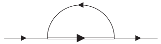
Figure 3: Diagrammatic representation of the fermion self-energy. See the caption of Fig. 1 for the other details.

For later purpose, we also evaluate the fermion self-energy,

$$\Sigma(ip^{\prime}_{0},{\bm{p}})=\frac{1}{\beta}\sum_{q^{\prime}_{0}}\int_{\bm{q}}\,D(ip^{\prime}_{0}+iq^{\prime}_{0},{\bm{p}}+{\bm{q}})G(iq^{\prime}_{0},{\bm{q}}),$$ (68)

whose diagrammatic representation is depicted in Fig. 3. Here, $G(iq^{\prime}_{0},{\bm{q}})=1/(iq^{\prime}_{0}-{\bm{q}}^{2}/2m+\mu)$ with $q^{\prime}_{0}=2\pi(n+1/2)/\beta$ is the fermion propagator and the summation over the fermionic Matsubara frequency leads to

$$\Sigma(ip^{\prime}_{0},{\bm{p}}) =\int_{-\infty}^{\infty}\!\frac{d\varepsilon}{\pi}\int_{\bm{q}}\left[f_{B}\!\left(\varepsilon+\tfrac{({\bm{p}}+{\bm{q}})^{2}}{4m}\right)+f_{F}\!\left(\tfrac{{\bm{q}}^{2}}{2m}\right)\right]$$

$$\quad\times\frac{\operatorname{Im}[D_{{\bm{p}}+{\bm{q}}}(\varepsilon-i0^{+})]}{ip^{\prime}_{0}+\mu-\varepsilon-\frac{({\bm{p}}+{\bm{q}})^{2}}{4m}+\frac{{\bm{q}}^{2}}{2m}}.$$ (69)

Because of $f_{F}(\varepsilon)\to ze^{-\beta\varepsilon}$ and $f_{B}(\varepsilon)\to z^{2}e^{-\beta\varepsilon}$ to the lowest order in fugacity, the first term in the square brackets is negligible and the integration over $\varepsilon$ can thus be performed, so that we obtain

$$\Sigma(ip^{\prime}_{0},{\bm{p}}) =\int_{\bm{q}}\,f_{F}\!\left(\tfrac{{\bm{q}}^{2}}{2m}\right)D\!\left(ip^{\prime}_{0}-\tfrac{{\bm{p}}^{2}}{2m}+\mu+\tfrac{({\bm{p}}-{\bm{q}})^{2}}{4m}\right)$$

$$\quad+O(z^{2}),$$ (70)

which has both real and imaginary parts at $O(z)$ Dusling:2013 ; Chafin:2013 .

The momentum distribution function of fermions for each spin component then follows from

$$f_{\bm{p}} =\frac{1}{\beta}\sum_{p^{\prime}_{0}}e^{ip^{\prime}_{0}0^{+}}[G(ip^{\prime}_{0},{\bm{p}})$$

$$\quad+G(ip^{\prime}_{0},{\bm{p}})\Sigma(ip^{\prime}_{0},{\bm{p}})G(ip^{\prime}_{0},{\bm{p}})+\cdots],$$ (71)

where the summation over the fermionic Matsubara frequency leads to

$$f_{\bm{p}} =f_{F}\!\left(\tfrac{{\bm{p}}^{2}}{2m}\right)+\int_{-\infty}^{\infty}\!\frac{d\varepsilon}{\pi}\,f_{F}\!\left(\varepsilon+\tfrac{{\bm{p}}^{2}}{2m}\right)$$

$$\quad\times\operatorname{Im}\!\left[\frac{\Sigma\bigl{(}\varepsilon+\frac{{\bm{p}}^{2}}{2m}-\mu-i0^{+},{\bm{p}}\bigr{)}}{(\varepsilon-i0^{+})^{2}}\right]+O(z^{3}).$$ (72)

Equivalently, it can also be expressed as

$$f_{\bm{p}} =Z_{\bm{p}}\,f_{F}\!\left(\tfrac{{\bm{p}}^{2}}{2m}\right)+f^{\prime}_{F}\!\left(\tfrac{{\bm{p}}^{2}}{2m}\right)\operatorname{Re}\!\left[\Sigma\!\left(\tfrac{{\bm{p}}^{2}}{2m}-\mu-i0^{+},{\bm{p}}\right)\right]$$

$$\quad+\mathrm{P}\int_{-\infty}^{\infty}\!\frac{d\varepsilon}{\pi}\,\frac{1}{\varepsilon}\,\frac{\partial}{\partial\varepsilon}\Bigl{\{}f_{F}\!\left(\varepsilon+\tfrac{{\bm{p}}^{2}}{2m}\right)$$

$$\qquad\times\operatorname{Im}\!\left[\Sigma\!\left(\varepsilon+\tfrac{{\bm{p}}^{2}}{2m}-\mu-i0^{+},{\bm{p}}\right)\right]\Bigr{\}}+O(z^{3}),$$ (73)

where $Z_{\bm{p}}=1+\operatorname{Re}[\Sigma^{\prime}({\bm{p}}^{2}/2m-\mu-i0^{+},{\bm{p}})]$ is the quasiparticle residue and ^′ denotes the partial derivative with respect to $\varepsilon$ at $\varepsilon=0$. In particular, the last term involving the imaginary part of the self-energy is responsible for the characteristic large-momentum tail of $\lim_{|{\bm{p}}|\to\infty}f_{\bm{p}}=\mathcal{C}/|{\bm{p}}|^{4}$ determined by the contact density Tan:2008a ; Tan:2008b ; Tan:2008c .

IV.2 Kinetic theory

The bulk viscosity is provided by $\zeta=\lim_{w\to i0^{+}}\zeta(w)$, which at $a\to\infty$ following from Eq. (IV.1) in the high-temperature limit was found to disagree with that derived from the kinetic theory both for $d=2,\,3$ Nishida:2019 ; Enss:2019 ; Hofmann:2020 . Here, we discuss that such discrepancies between the Kubo formalism and the kinetic theory for the bulk viscosity are attributed to the fact that the quasiparticle approximation assumed by the latter breaks down even in the high-temperature limit where the fermion self-energy becomes small.

The bulk viscosity in the high-temperature limit was computed in Refs. Dusling:2013 ; Chafin:2013 by employing the Landau kinetic equation for quasiparticles,

$$\frac{\partial f_{\bm{p}}}{\partial t}+\frac{\partial E_{\bm{p}}}{\partial{\bm{p}}}\cdot\frac{\partial f_{\bm{p}}}{\partial{\bm{r}}}-\frac{\partial E_{\bm{p}}}{\partial{\bm{r}}}\cdot\frac{\partial f_{\bm{p}}}{\partial{\bm{p}}}=\left(\frac{\partial f_{\bm{p}}}{\partial t}\right)_{\mathrm{coll}},$$ (74)

where

$$E_{\bm{p}}[f(t,{\bm{r}})]=\frac{{\bm{p}}^{2}}{2m}$$

$$\quad+\operatorname{Re}\!\left[\Sigma\!\left(\tfrac{{\bm{p}}^{2}}{2m}-\mu-i0^{+},{\bm{p}}\right)\right]\Big{|}_{f_{F}({\bm{q}}^{2}/2m)\to f_{\bm{q}}(t,{\bm{r}})}$$ (75)

is the quasiparticle energy functional of the nonequilibrium distribution function and its on-shell self-energy correction is obtained from the real part of Eq. (IV.1) with the Fermi-Dirac distribution function replaced by the nonequilibrium distribution function. In particular, the scale invariance breaking in the quasiparticle energy due to its self-energy correction was found to be essential to a nonvanishing bulk viscosity Dusling:2013 ; Chafin:2013 . However, we consider that such a kinetic equation is not fully grounded because the self-energy in Eq. (IV.1) has both real and imaginary parts at $O(z)$. Namely, if the real part of the self-energy is essential to the bulk viscosity, its imaginary part being at the same order in fugacity is non-negligible so as to invalidate the quasiparticle approximation, i.e., replacing the fermion spectral function by a $\delta$ function on which the kinetic equation is founded Kita:2010 .

In order to further support our consideration, let us study the equilibrium distribution function resulting from the kinetic equation. Because the collision term in Eq. (74) must be canceled under the conservation of quasiparticle energies Baym-Pethick , the equilibrium distribution function in the rest frame obeys the self-consistent equation of

$$f_{\bm{p}}=\frac{1}{e^{\beta(E_{\bm{p}}[f]-\mu)}+1}.$$ (76)

By substituting the quasiparticle energy in Eq. (IV.2) and expanding the right-hand side in terms of fugacity iteratively, we obtain

$$f_{\bm{p}} =f_{F}\!\left(\tfrac{{\bm{p}}^{2}}{2m}\right)+f^{\prime}_{F}\!\left(\tfrac{{\bm{p}}^{2}}{2m}\right)\operatorname{Re}\!\left[\Sigma\!\left(\tfrac{{\bm{p}}^{2}}{2m}-\mu-i0^{+},{\bm{p}}\right)\right]$$

$$\quad+O(z^{3}),$$ (77)

where two contributions are found to be missing from the microscopic distribution function in Eq. (IV.1). One is the factor of the quasiparticle residue, whereas the other is the whole term involving the imaginary part of the self-energy. Furthermore, because all thermodynamic variables in the kinetic theory are expressed in terms of the distribution function Baym-Pethick , they also differ from the microscopic ones in the quantum virial expansion. Therefore, the Landau kinetic equation employed in Refs. Dusling:2013 ; Chafin:2013 is incapable of describing physics at the order where the self-energy contributes because its imaginary part neglected therein is actually non-negligible. We consider that this constitutes the origin of the discrepancy between the Kubo formalism and the kinetic theory for the bulk viscosity.

V Summary

The standard Kubo formula for the bulk viscosity presented in Eq. (1) has flaws to give rise to unphysical divergences at zero frequency. They are however resolved with the corrected Kubo formula Mori:1962 ; Luttinger:1964 ; Bradlyn:2012 , which has been known since long ago but is not well appreciated by the literature in the context of ultracold atom physics. After carefully rederiving the Kubo formula for the frequency-dependent complex bulk viscosity as well as its sum rule, we found that the sum rule for two-component fermions with a zero-range interaction in two and three dimensions [Eq. (44)] coincides with that derived in Ref. Taylor:2010 , although we do not fully agree with the derivation therein because of the neglected pressure fluctuations.

The Kubo formula can be evaluated unambiguously, in particular, by working with the complex bulk viscosity on the upper-half plane of complex frequency. We then confirmed that the bulk viscosity spectral function indeed vanishes at an arbitrary frequency in the free and unitarity limits and at a lower frequency than the binding energy of dimers in the dimer limit [Eq. (III.3)] without the unphysical divergences at zero frequency.

In the high-temperature limit, the bulk viscosity spectral function in the quantum virial expansion [Eq. (IV.1)] was reproduced with our diagrammatic method. We also discussed that the Landau kinetic equation employed in Refs. Dusling:2013 ; Chafin:2013 to compute the bulk viscosity is not fully grounded even in the high-temperature limit where the fermion self-energy becomes small. This is because the self-energy has both real and imaginary parts at the same order in fugacity so as to invalidate the quasiparticle approximation, i.e., replacing the fermion spectral function by a $\delta$ function on which the kinetic equation is founded. We consider that this constitutes the origin of the recently found discrepancy between the Kubo formalism and the kinetic theory for the bulk viscosity Nishida:2019 ; Enss:2019 ; Hofmann:2020 .

Appendix A Kubo’s canonical correlation function

In this Appendix, we present some useful formulas and their detailed derivations regarding Kubo’s canonical correlation function Kubo:1957 .

A.1 Derivation of Eq. (12)

First, by multiplying the response function defined in Eq. (10) by $iw$ and using $iwe^{iwt}=\partial_{t}e^{iwt}$, the temporal integration by parts leads to

$$iwR_{\mathcal{J}_{i}\mathcal{J}_{j}}(w,{\bm{k}})=-i\int\!d{\bm{r}}\,e^{-i{\bm{k}}\cdot{\bm{r}}}\langle[\hat{\mathcal{J}}_{i}(0,{\bm{r}}),\hat{\mathcal{J}}_{j}(0,{\bm{0}})]\rangle-i\int_{0}^{\infty}\!dt\int\!d{\bm{r}}\,e^{iwt-i{\bm{k}}\cdot{\bm{r}}}\langle[\partial_{t}\hat{\mathcal{J}}_{i}(t,{\bm{r}}),\hat{\mathcal{J}}_{j}(0,{\bm{0}})]\rangle.$$ (78)

Here, the first term turns out to vanish because of $[\hat{\mathcal{J}}_{i}({\bm{r}}),\hat{\mathcal{J}}_{j}({\bm{r}}^{\prime})]=[\hat{\mathcal{J}}_{j}({\bm{r}})\partial_{i}+\hat{\mathcal{J}}_{i}({\bm{r}}^{\prime})\partial_{j}]\delta({\bm{r}}-{\bm{r}}^{\prime})/(im)$ Nishida:2007 . Then, by using the momentum continuity equation (13), the spatial integration by parts leads to

$$iwR_{\mathcal{J}_{i}\mathcal{J}_{j}}(w,{\bm{k}})=-\frac{k_{k}}{m}\int_{0}^{\infty}\!dt\int\!d{\bm{r}}\,e^{iwt-i{\bm{k}}\cdot{\bm{r}}}\langle[\hat{\pi}_{ik}(t,{\bm{r}}),\hat{\mathcal{J}}_{j}(0,{\bm{0}})]\rangle.$$ (79)

After using the spacetime translational invariance, the integrand can be rewritten as

$$\langle[\hat{\pi}_{ik}(0,{\bm{0}}),\hat{\mathcal{J}}_{j}(-t,-{\bm{r}})]\rangle =\langle[\hat{\pi}_{ik}(0,{\bm{0}})\hat{\mathcal{J}}_{j}(-t,-{\bm{r}})-\hat{\pi}_{ik}(0,{\bm{0}})e^{-\beta\hat{H}}\hat{\mathcal{J}}_{j}(-t,-{\bm{r}})e^{\beta\hat{H}}]\rangle$$

$$=-\int_{0}^{\beta}\!d\tau\,\partial_{\tau}\langle\hat{\pi}_{ik}(0,{\bm{0}})e^{-\tau\hat{H}}\hat{\mathcal{J}}_{j}(-t,-{\bm{r}})e^{\tau\hat{H}}\rangle$$

$$=i\int_{0}^{\beta}\!d\tau\,\langle\hat{\pi}_{ik}(0,{\bm{0}})\partial_{t}\hat{\mathcal{J}}_{j}(-t+i\tau,-{\bm{r}})\rangle,$$ (80)

because the number operator $\hat{N}$ commutes with the other operators. Then, by using the momentum continuity equation (13) again, the spatial integration by parts leads to

$$iwR_{\mathcal{J}_{i}\mathcal{J}_{j}}(w,{\bm{k}})=-\frac{k_{k}k_{l}}{m^{2}}\int_{0}^{\infty}\!dt\int\!d{\bm{r}}\,e^{iwt-i{\bm{k}}\cdot{\bm{r}}}\int_{0}^{\beta}\!d\tau\,\langle\delta\hat{\pi}_{ik}(0,{\bm{0}})\delta\hat{\pi}_{jl}(-t+i\tau,-{\bm{r}})\rangle,$$ (81)

where the expectation value needs to be subtracted from the operator to ensure that boundary contributions at spatial infinity vanish under the clustering property:

$$\lim_{|{\bm{r}}|\to\infty}\langle\delta\hat{\pi}_{ik}(0,{\bm{0}})\delta\hat{\pi}_{jl}(-t+i\tau,-{\bm{r}})\rangle=\lim_{|{\bm{r}}|\to\infty}\langle\delta\hat{\pi}_{ik}(0,{\bm{0}})\rangle\langle\delta\hat{\pi}_{jl}(-t+i\tau,-{\bm{r}})\rangle=0.$$ (82)

Finally, by using the spacetime translational invariance again and comparing the outcome with the canonical correlation function defined in Eq. (II.1), we arrive at Eq. (12).

A.2 Derivation of Eq. (34)

First, by substituting the modified stress tensor operator defined in Eq. (33) into the right-hand side of Eq. (34), we obtain

$$K_{\tilde{\pi}\tilde{\pi}}(w,{\bm{0}}) =K_{\pi\pi}(w,{\bm{0}})-2\left(\frac{\partial p}{\partial\mathcal{N}}\right)_{\mathcal{E}}K_{\mathcal{N}\pi}(w,{\bm{0}})-2\left(\frac{\partial p}{\partial\mathcal{E}}\right)_{\mathcal{N}}K_{\mathcal{H}\pi}(w,{\bm{0}})$$

$$\quad+\left(\frac{\partial p}{\partial\mathcal{N}}\right)_{\mathcal{E}}\left[\left(\frac{\partial p}{\partial\mathcal{N}}\right)_{\mathcal{E}}K_{\mathcal{N}\mathcal{N}}(w,{\bm{0}})+\left(\frac{\partial p}{\partial\mathcal{E}}\right)_{\mathcal{N}}K_{\mathcal{N}\mathcal{H}}(w,{\bm{0}})\right]$$

$$\quad+\left(\frac{\partial p}{\partial\mathcal{E}}\right)_{\mathcal{N}}\left[\left(\frac{\partial p}{\partial\mathcal{N}}\right)_{\mathcal{E}}K_{\mathcal{H}\mathcal{N}}(w,{\bm{0}})+\left(\frac{\partial p}{\partial\mathcal{E}}\right)_{\mathcal{N}}K_{\mathcal{H}\mathcal{H}}(w,{\bm{0}})\right],$$ (83)

because $\hat{N}$ and $\hat{H}$ are conserved. Then, by using the following properties of the canonical correlation function,

$$K_{\mathcal{N}\mathcal{O}}(w,{\bm{0}}) =-\frac{1}{iw}\left(\frac{\partial\langle\hat{\mathcal{O}}({\bm{0}})\rangle}{\beta\partial\mu}\right)_{\beta},$$ (84)

$$K_{\mathcal{H}\mathcal{O}}(w,{\bm{0}}) =\frac{1}{iw}\left(\frac{\partial\langle\hat{\mathcal{O}}({\bm{0}})\rangle}{\partial\beta}\right)_{\beta\mu},$$ (85)

for $\langle\hat{\mathcal{N}}({\bm{r}})\rangle=\mathcal{N}$, $\langle\hat{\mathcal{H}}({\bm{r}})\rangle=\mathcal{E}$, and $\langle\hat{\pi}({\bm{r}})\rangle=p$, the thermodynamic identities lead to

$$K_{\tilde{\pi}\tilde{\pi}}(w,{\bm{0}}) =K_{\pi\pi}(w,{\bm{0}})+\frac{2}{iw}\left(\frac{\partial p}{\partial\mathcal{N}}\right)_{\mathcal{E}}\left(\frac{\partial p}{\beta\partial\mu}\right)_{\beta}-\frac{2}{iw}\left(\frac{\partial p}{\partial\mathcal{E}}\right)_{\mathcal{N}}\left(\frac{\partial p}{\partial\beta}\right)_{\beta\mu}$$

$$\quad-\frac{1}{iw}\left(\frac{\partial p}{\partial\mathcal{N}}\right)_{\mathcal{E}}\left[\left(\frac{\partial p}{\partial\mathcal{N}}\right)_{\mathcal{E}}\left(\frac{\partial\mathcal{N}}{\beta\partial\mu}\right)_{\beta}+\left(\frac{\partial p}{\partial\mathcal{E}}\right)_{\mathcal{N}}\left(\frac{\partial\mathcal{E}}{\beta\partial\mu}\right)_{\beta}\right]$$

$$\quad+\frac{1}{iw}\left(\frac{\partial p}{\partial\mathcal{E}}\right)_{\mathcal{N}}\left[\left(\frac{\partial p}{\partial\mathcal{N}}\right)_{\mathcal{E}}\left(\frac{\partial\mathcal{N}}{\partial\beta}\right)_{\beta\mu}+\left(\frac{\partial p}{\partial\mathcal{E}}\right)_{\mathcal{N}}\left(\frac{\partial\mathcal{E}}{\partial\beta}\right)_{\beta\mu}\right]$$

$$=K_{\pi\pi}(w,{\bm{0}})+\frac{1}{iw}\left(\frac{\partial p}{\partial\mathcal{N}}\right)_{\mathcal{E}}\frac{\mathcal{N}}{\beta}+\frac{1}{iw}\left(\frac{\partial p}{\partial\mathcal{E}}\right)_{\mathcal{N}}\frac{\mathcal{E}+p}{\beta}.$$ (86)

Finally, by using the sound velocity in Eq. (27) and comparing the outcome with the frequency-dependent complex bulk viscosity defined in Eq. (32), we arrive at Eq. (34).

A.3 Comparison of Eq. (32) with Ref. Bradlyn:2012

First, by using $e^{iwt}=\partial_{t}e^{iwt}/iw$ in the canonical correlation function in Eq. (32), the temporal integration by parts leads to

$$\zeta(w)=\frac{mc_{s}^{2}\mathcal{N}}{iw}-\frac{1}{iw}\int\!d{\bm{r}}\int_{0}^{\beta}\!d\tau\,\langle\delta\hat{\pi}(-i\tau,{\bm{r}})\delta\hat{\pi}(0,{\bm{0}})\rangle-\frac{1}{iw}\int_{0}^{\infty}\!dt\int\!d{\bm{r}}\,e^{iwt}\int_{0}^{\beta}\!d\tau\,\langle\partial_{t}\delta\hat{\pi}(t-i\tau,{\bm{r}})\delta\hat{\pi}(0,{\bm{0}})\rangle.$$ (87)

Then, the integral over $\tau$ in the last term can be rewritten as

$$\int_{0}^{\beta}\!d\tau\,\langle\partial_{t}\delta\hat{\pi}(t-i\tau,{\bm{r}})\delta\hat{\pi}(0,{\bm{0}})\rangle =i\int_{0}^{\beta}\!d\tau\,\partial_{\tau}\langle e^{\tau\hat{H}}\delta\hat{\pi}(t,{\bm{r}})e^{-\tau\hat{H}}\delta\hat{\pi}(0,{\bm{0}})\rangle$$

$$=i\langle[e^{\beta\hat{H}}\delta\hat{\pi}(t,{\bm{r}})e^{-\beta\hat{H}}\delta\hat{\pi}(0,{\bm{0}})-\delta\hat{\pi}(t,{\bm{r}})\delta\hat{\pi}(0,{\bm{0}})]\rangle$$

$$=-i\langle[\delta\hat{\pi}(t,{\bm{r}}),\delta\hat{\pi}(0,{\bm{0}})]\rangle$$

$$=-i\langle[\hat{\pi}(t,{\bm{r}}),\hat{\pi}(0,{\bm{0}})]\rangle,$$ (88)

so that we obtain

$$\zeta(w)=\frac{mc_{s}^{2}\mathcal{N}}{iw}-\frac{1}{iw}\int\!d{\bm{r}}\int_{0}^{\beta}\!d\tau\,\langle\delta\hat{\pi}(-i\tau,{\bm{r}})\delta\hat{\pi}(0,{\bm{0}})\rangle+\frac{R_{\pi\pi}(w,{\bm{0}})}{iw}.$$ (89)

Here, the last term is the stress-stress response function, whereas the first and second terms evidently correspond to the inverse compressibility and equal-time commutator (“contact”) terms of Ref. Bradlyn:2012 , respectively.

Actually, the first and second terms are combined into the sum rule in Eq. (II.4), so that the frequency-dependent complex bulk viscosity can also be expressed as

$$\zeta(w)=\frac{R_{\pi\pi}(w,{\bm{0}})}{iw}-\frac{1}{iw}\int_{-\infty}^{\infty}\!\frac{d\omega}{\pi}\,\zeta(\omega+i0^{+}).$$ (90)

This is the formula employed in Sec. III.2. Its real part for $w\to\omega+i0^{+}$ then reads

$$\operatorname{Re}[\zeta(\omega+i0^{+})]=\frac{\operatorname{Im}[R_{\pi\pi}(\omega+i0^{+},{\bm{0}})]}{\omega}-\pi\delta(\omega)\left[\operatorname{Re}[R_{\pi\pi}(i0^{+},{\bm{0}})]-\int_{-\infty}^{\infty}\!\frac{d\omega^{\prime}}{\pi}\zeta(\omega^{\prime}+i0^{+})\right],$$ (91)

whose last term unless canceled is missing from the standard Kubo formula for the bulk viscosity in Eq. (1).

References

- (1) The BCS-BEC Crossover and the Unitary Fermi Gas, edited by W. Zwerger, Lecture Notes in Physics Vol. 836 (Springer, Berlin, Heidelberg, 2012).
- (2) T. Mehen, I. W. Stewart, and M. B. Wise, “Conformal invariance for non-relativistic field theory,” Phys. Lett. B 474, 145-152 (2000).
- (3) D. T. Son and M. Wingate, “General coordinate invariance and conformal invariance in nonrelativistic physics: Unitary Fermi gas,” Ann. Phys. (NY) 321, 197-224 (2006).
- (4) Y. Nishida and D. T. Son, “Nonrelativistic conformal field theories,” Phys. Rev. D 76, 086004 (2007).
- (5) D. T. Son, “Vanishing bulk viscosities and conformal invariance of the unitary Fermi gas,” Phys. Rev. Lett. 98, 020604 (2007).
- (6) E. Taylor and M. Randeria, “Viscosity of strongly interacting quantum fluids: Spectral functions and sum rules,” Phys. Rev. A 81, 053610 (2010).
- (7) T. Enss, R. Haussmann, and W. Zwerger, “Viscosity and scale invariance in the unitary Fermi gas,” Ann. Phys. (NY) 326, 770-796 (2011).
- (8) Y. Nishida, “Viscosity spectral functions of resonating fermions in the quantum virial expansion,” Ann. Phys. (NY) 410, 167949 (2019).
- (9) T. Enss, “Bulk viscosity and contact correlations in attractive Fermi gases,” Phys. Rev. Lett. 123, 205301 (2019).
- (10) J. Hofmann, “High-temperature expansion of the viscosity in interacting quantum gases,” Phys. Rev. A 101, 013620 (2020).
- (11) M. Martinez and T. Schäfer, “Hydrodynamic tails and a fluctuation bound on the bulk viscosity,” Phys. Rev. A 96, 063607 (2017).
- (12) K. Fujii and Y. Nishida, “Hydrodynamics with spacetime-dependent scattering length,” Phys. Rev. A 98, 063634 (2018).
- (13) B. Bradlyn, M. Goldstein, and N. Read, “Kubo formulas for viscosity: Hall viscosity, Ward identities, and the relation with conductivity,” Phys. Rev. B 86, 245309 (2012).
- (14) H. Mori, “Collective motion of particles at finite temperatures,” Prog. Theor. Phys. 28, 763-783 (1962).
- (15) J. M. Luttinger, “Theory of thermal transport coefficients,” Phys. Rev. 135, A1505-A1514 (1964).
- (16) See, for example, A. Altland and B. D. Simons, Condensed Matter Field Theory, 2nd ed. (Cambridge University Press, Cambridge, U.K., 2010).
- (17) R. Kubo, “Statistical-mechanical theory of irreversible processes. I. General theory and simple applications to magnetic and conduction problems,” J. Phys. Soc. Jpn. 12, 570-586 (1957).
- (18) See, for example, L. D. Landau and E. M. Lifshitz, Fluid Mechanics, 2nd ed. (Butterworth-Heinemann, Oxford, 1987).
- (19) E. Braaten and L. Platter, “Exact relations for a strongly interacting Fermi gas from the operator product expansion,” Phys. Rev. Lett. 100, 205301 (2008).
- (20) S. Tan, “Energetics of a strongly correlated Fermi gas,” Ann. Phys. (NY) 323, 2952-2970 (2008).
- (21) S. Tan, “Large momentum part of a strongly correlated Fermi gas,” Ann. Phys. (NY) 323, 2971-2986 (2008).
- (22) S. Tan, “Generalized virial theorem and pressure relation for a strongly correlated Fermi gas,” Ann. Phys. (NY) 323, 2987-2990 (2008).
- (23) E. Taylor and M. Randeria, “Apparent low-energy scale invariance in two-dimensional Fermi gases,” Phys. Rev. Lett. 109, 135301 (2012).
- (24) C. A. R. Sá de Melo, M. Randeria, and J. R. Engelbrecht, “Crossover from BCS to Bose superconductivity: Transition temperature and time-dependent Ginzburg-Landau theory,” Phys. Rev. Lett. 71, 3202 (1993).
- (25) X.-J. Liu, “Virial expansion for a strongly correlated Fermi system and its application to ultracold atomic Fermi gases,” Phys. Rep. 524, 37-83 (2013).
- (26) K. Dusling and T. Schäfer, “Bulk viscosity and conformal symmetry breaking in the dilute Fermi gas near unitarity,” Phys. Rev. Lett. 111, 120603 (2013).
- (27) C. Chafin and T. Schäfer, “Scale breaking and fluid dynamics in a dilute two-dimensional Fermi gas,” Phys. Rev. A 88, 043636 (2013).
- (28) T. Kita, “Introduction to nonequilibrium statistical mechanics with quantum field theory,” Prog. Theor. Phys. 123, 581-658 (2010).
- (29) P. Massignan, G. M. Bruun, and H. Smith, “Viscous relaxation and collective oscillations in a trapped Fermi gas near the unitarity limit,” Phys. Rev. A 71, 033607 (2005).
- (30) G. M. Bruun and H. Smith, “Viscosity and thermal relaxation for a resonantly interacting Fermi gas,” Phys. Rev. A 72, 043605 (2005).
- (31) G. M. Bruun, “Shear viscosity and spin-diffusion coefficient of a two-dimensional Fermi gas,” Phys. Rev. A 85, 013636 (2012).
- (32) T. Schäfer, “Shear viscosity and damping of collective modes in a two-dimensional Fermi gas,” Phys. Rev. A 85, 033623 (2012).
- (33) See, for example, G. Baym and C. Pethick, Landau Fermi-Liquid Theory: Concepts and Applications (Wiley, New York, 1991).