Deep learning black hole metrics from shear viscosity

Abstract

Based on AdS/CFT correspondence, we build a deep neural network to learn black hole metrics from the complex frequency-dependent shear viscosity. The network architecture provides a discretized representation of the holographic renormalization group flow of the shear viscosity and can be applied to a large class of strongly coupled field theories. Given the existence of the horizon and guided by the smoothness of spacetime, we show that Schwarzschild and Reissner-Nordström metrics can be learned accurately. Moreover, we illustrate that the generalization ability of the deep neural network can be excellent, which indicates that by using the black hole spacetime as a hidden data structure, a wide spectrum of the shear viscosity can be generated from a narrow frequency range. These results are further generalized to an Einstein-Maxwell-dilaton black hole. Our work might not only suggest a data-driven way to study holographic transports but also shed some light on holographic duality and deep learning.

Introduction.—Renormalization group (RG) is a physical scheme to understand various emergent phenomena in the world through iterative coarse graining Kadanoff1966 ; Wilson74 ; Wilson83 ; Polchinski84 . Deep learning (DL) is the core algorithm of the recent wave of artificial intelligence Sejnowski2018 . It has been suggested that RG and DL might have a logic in common Wen16 ; Mehta1401 and their relation has attracted a lot of interest Beny13 ; Saremi13 ; Paul1412 ; Braddea1610 ; Lin1608 ; Ringel1704 ; Oprisa1705 ; Foreman1710 ; Iso1801 ; Wang1802 .

RG is believed to be one of the key elements to understand quantum gravity. In particular, by anti-de Sitter/conformal field theory (AdS/CFT) correspondence Maldacena97 ; Gubser98 ; Witten98 ; Susskind98 , a strongly coupled quantum critical theory in the d-dimensional spacetime is reorganized along the RG scale, inducing a classical theory of gravity in the (d+1)-dimensional AdS spacetime. RG is not the only connection between DL and gravity. Through the study of tensor networks Bridgeman1603 ; Scholl2011 ; Vidal2011 , especially the multi-scale entanglement renormalization ansatz (MERA) Vidal0512 , it has been realized that the way the geometry is emergent from field theories usually involves the network and optimization, which are two important ingredients of DL.

Because of these connections, the deep neural network (DNN) may be capable of providing a research platform for holographic duality Shu1705 ; You1709 ; Hashimoto1802 ; Hashimoto1809 ; You1903 ; Hashimoto1903 ; Hartnoll1906 ; Tan1908 . One can expect at least two benefits: It is helpful to understand how the spacetime emerges and can be used to build a data-driven phenomenological model for strongly coupled field theories. The latter was initiated in Hashimoto1802 , where the inverse problem of the AdS/CFT is studied, that is, how to reconstruct the spacetime metric from the given field theory data by the DNN which implements the AdS/CFT. Subsequently, the so-called AdS/DL correspondence is applied to learn the bulk metric from the lattice QCD data of the finite-temperature chiral condensate. Interestingly, the emergent metric exhibits both a black hole horizon and an IR wall with finite height, signaling the crossover of QCD thermal phases Hashimoto1809 .

Let us briefly introduce the prototype of AdS/DL (i.e., the first numerical experiment in Hashimoto1802 ). It establishes the architecture of the DNN according to the discretized equation of motion of the $\phi^{4}$ theory minimally coupled to gravity. The training data are the one-point function and the conjugate source with a label determined by the near-horizon scalar field. The target of learning is the metric of the Schwarzschild black hole. A key technique is to design the regularization by which the emergent metric is favored to be smooth. It is found that the DNN performs better near the boundary than near the horizon where the relative error is around 30%. In Tan1908 , it has been attempted to learn the Reissner-Nordström (RN) metric by AdS/DL but the mean square error (MSE) ranges from $\mathcal{O}\left(10^{-3}\right)$ to $\mathcal{O}\left(10^{-1}\right)$. Importantly, it was revealed that the form of the regularization term must be fine-tuned for different metrics. This suggests that their DNN may not find the target metric if it is unknown previously, since it is difficult to judge which is closer to the target metric under different regularizations.

In this paper, we will extend the physical range of the AdS/DL nontrivially and illustrate that it can be realized without previous technical problems. Our strategies are as follows. First, AdS/CFT is almost customized for the computation of the transports of strongly coupled quantum critical systems at finite temperatures ZaanenBook . In particular, the application of holography is anchored partially in the prediction of the nearly perfect fluidity KSS , which has been observed in the hot quark gluon plasmas and cold unitary Fermi gases Schaefer0904 . With these in mind, we adapt the complex frequency-dependent shear viscosity as the given field theory data. Second, we propose to build the DNN according to the holographic RG flow of the shear viscosity. Up to the holographic renormalization, this flow was presented in the well-known holographic membrane paradigm Liu0809 ; Strominger1006 , which interpolates the standard AdS/CFT correspondence and the classical black hole membrane paradigm smoothly Thorne86 ; Wilczek97 . Third, we assume the existence of the horizon, which will reduce the learning difficulties. Fourth, the system error in Hashimoto1802 comes from adding labels on the data and introducing the regularization. Because the horizon value of the shear response is completely determined by the regularity analysis on the horizon, we can generate the data by the flow from IR to UV. The direction of information transfer is contrary to Hashimoto1802 ; Hashimoto1809 and there is no error caused by the labels of the data. Fifth, we still use the regularization to guide the network to find a smooth metric. However, our training process has two stages and the regularization is only required in the first stage, so we can choose any regularization term as long as it leads to a smaller loss in the second stage. Finally, we will discuss possible extensions and physical implications.

From RG flow to DNN.—Suppose that a strongly coupled field theory is dual to the (3+1)-dimensional Einstein gravity minimally coupled with matter, which admits a homogeneous and isotropic (along the field theory directions) black hole solution with the metric ansatz

$$ds^{2}=-g_{tt}(r)dt^{2}+g_{rr}(r)dr^{2}+g_{xx}(r)d\vec{x}^{2}.$$ (1)

When the black hole is perturbed by time-dependent sources, the shear mode $\left(\delta g\right)_{\;x_{2}}^{x_{1}}=h(r)e^{-i\omega t}$ of the gravitational wave is controlled by the equation of motion

$$\frac{1}{\sqrt{-g}}\partial_{r}(\sqrt{-g}g^{rr}\partial_{r}h)+g^{tt}\omega^{2}h=0,$$ (2)

provided that the graviton is massless Hartnoll1601 . In the Hamiltonian form, the wave equation can be written as

$$\Pi = -\sqrt{-g}g^{rr}\partial_{r}h,$$ (3)

$$\partial_{r}\Pi = \sqrt{-g}g^{rr}g^{tt}\omega^{2}h,$$ (4)

where $\Pi$ is the momentum conjugate to the field $h$. Consider the foliation in the $r$-direction and define the shear response function $\chi=\Pi/(i\omega h)$ on each cutoff surface. Substituting Eq. (3) into Eq. (4), one can obtain

$$\partial_{r}\chi-i\omega\sqrt{\frac{g_{rr}}{g_{tt}}}\left(\frac{\chi^{2}}{g_{xx}}-g_{xx}\right)=0.$$ (5)

Note that this radial flow equation has been derived in Liu0809 where the DC limit is focused on. We will study the frequency-dependent behavior.

Applying the regularity of $\chi$ on the horizon, one can read off the horizon value of $\chi$ directly

$$\chi(r_{h})=g_{xx}(r_{h}),$$ (6)

where $r_{h}$ is the horizon radius. Taking Eq. (6) as the IR boundary condition, the flow equation can be integrated to the UV boundary. However, it should be pointed out that the response function $\chi$ on the UV boundary is not equal to the shear viscosity $\eta$ of the boundary field theory. In the Supplementary Material (SM), we will clarify the relation between them using the Kubo formula of the complex frequency-dependent shear viscosity Read1207 ; Wu2015 and the holographic renormalization Henningson9806 ; HJ . It can be found that for a large class of holographic models, including the Einstein-Maxwell theory which will be studied below, the relation is

$$\eta(\omega)=\left.\chi(\omega,r)+i\omega r\right|_{r\rightarrow\infty}.$$ (7)

In the metric ansatz (1), $g_{xx}$ can be fixed as $r^{2}$ without loss of generality but $g_{tt}$ and $g_{rr}$ are independent in general. However, there are some black holes which share the feature $g_{tt}g_{rr}=1$, indicating that the radial pressure is the negative of the energy density Jacobson0707 . For simplicity, we will consider this situation first and return to the more general case later. Thus, the metric ansatz can be reduced to

$$ds^{2}=\frac{1}{z^{2}}\left[-f(z)dt^{2}+\frac{1}{f(z)}dz^{2}+d\vec{x}^{2}\right],$$ (8)

where we have used the coordinate $z=r_{h}/r$ so that the horizon is located at $z=1$ and the boundary at $z=0$. Accordingly, Eq. (5) can be rewritten as

$$\left(\eta-\frac{i\omega}{z}\right)^{\prime}+\frac{i\omega}{f}\left[z^{2}\left(\eta-\frac{i\omega}{z}\right)^{2}-\frac{1}{z^{2}}\right]=0,$$ (9)

where we have set $r_{h}=1$ and the prime denotes the derivative with respect to $z$. Note that we have replaced $\chi(\omega,z)$ with $\eta(\omega,z)-i\omega/z$ from IR to UV. Compared to Eq. (7) where the replacement occurs only on the UV, we have found that this technique reduces the discretized error considerably. The radially varying function $\eta(\omega,z)$ can be referred to the holographic RG flow of the shear viscosity. In the following, we will build a DNN according to the flow equation (9).

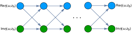
Figure 1: The architecture of the DNN. The green and blue nodes have $N$ layers, which propagate the shear viscosity from IR to UV by discretized RG flow equations (11). The arrows indicate the direction of information transfer.

FIG. 1 is a schematic diagram of the DNN. The $N$ deep layers are located by discretizing the radial direction

$$z(n)=z_{b}+n\Delta z,\;\Delta z=\frac{z_{h}-z_{b}}{N},$$ (10)

where $z_{b}$ ($z_{h}$) is the UV (IR) cutoff and the integer $n$ belongs to $\left[1,N\right]$. The trainable weights of the DNN represent the discretized metrics. The input is $\eta(\omega,z_{h})$ and the output is $\eta(\omega,z_{b})$. The information is transferred from the $N$th layer (IR) to the $1$th layer (UV). The propagation rule of $\eta(\omega,z)$ between layers is determined by the discretized representation of Eq. (9):

$$\text{{Re}}\eta\left(z+\Delta z\right) = \text{{Re}}\eta\left(z\right)\left[1+\Delta z\frac{2\omega z^{2}}{f\left(z\right)}\left(\text{{Im}}\eta\left(z\right)-\frac{\omega}{z}\right)\right],$$

$$\text{{Im}}\eta\left(z+\Delta z\right) = \text{{Im}}\eta\left(z\right)+\Delta z\frac{\omega z^{2}}{f\left(z\right)}\Big{[}\frac{1-f(z)}{z^{4}}$$ (11)

$$-\left(\text{{Re}}\eta\left(z\right)\right)^{2}+\left(\text{{Im}}\eta\left(z\right)-\frac{\omega}{z}\right)^{2}\Big{]}.$$

Here we have separated the discretized flow equation into real and imaginary parts for the convenience in DL.

The loss function we choose is the $L^{2}$-norm

$$L_{\mathrm{DNN}}=\sum_{\mathrm{data}}\left|\eta(\omega,z_{b})-\bar{\eta}(\omega,z_{b})\right|^{2},$$ (12)

up to a regularization term, if existent. Here $\eta$ represents the input data and $\bar{\eta}$ is what the DNN generates.

We need a regularization term which can guide the DNN to find a smooth black hole metric. In principle, the form of the regularization term can be arbitrary as long as it can reduce the final loss. In practice, our regularization term is specified as

$$L_{\text{{REG}}} = c_{1}\sum_{n=1}^{N-1}\frac{1}{z(n)^{c_{2}}}\left[f(z(n+1))-f(z(n))\right]^{2}$$ (13)

$$+c_{3}\left[f(z(N))-0\right]^{2},$$

where the two parts are designed for the smoothness of the metric and the existence of the horizon, respectively. Three hyperparameters $c_{1},c_{2}$, and $c_{3}$ are introduced.

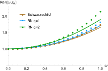
Figure 2: The data of the shear viscosity generated by different metrics. (a) and (b) denote the real and imaginary parts, respectively. The curves are generated by the continuous holographic RG flow equation of the shear viscosity, while the markers are generated by the discretized equation.

Generated data and discretized error.—We specify the discretized RG flow and hence the DNN by setting $z_{b}=0.01$, $z_{h}=0.99$, and $N=10$. Using the discretized flow equation (11) with the IR boundary condition $\eta(\omega,z_{h})=1+i\omega$ and the target metric, we can generate the data required by DL. Here we consider the two most famous black holes, i.e. the Schwarzschild and RN. They are characterized respectively by the functions

$$f(z) = 1-z^{3},$$ (14)

$$f(z) = 1-z^{3}-\frac{q^{2}z^{3}}{4}+\frac{q^{2}z^{4}}{4},$$ (15)

where $q$ is the charge density. We generate 2000 data $(\omega,\ \eta(\omega,z_{b}))$ with even frequency spacing. The training set and validation set account for 90% and 10%, respectively. In Fig. (2), we compare the data with the ones generated by numerically solving the continuous flow equation of the shear viscosity. It is found that the discretized error is small when the target is the Schwarzschild metric, and increases with the frequency and the charge density. The discretized error can be reduced by adding more layers but it requires powerful computing capabilities. As a proof of principle, here we simply assume that the discretized error does not affect our results qualitatively.

Emergence and generalization.—With the data in hand, we will train the DNN and extract the weights. The training scheme will be given in the SM. In TABLE S.1, we list the training reports after two training stages of various numerical experiments. Among others, it is shown that from the dataset with $\omega\in(0,1]$, the Schwarzschild and RN metrics can be learned with high accuracy: the mean relative error (MRE) is around $0.1\%$. Note that the MSE is $\mathcal{O}\left(10^{-7}\right)$. The target and learned metrics have been plotted in FIG. (3.a).

Hereto, we almost naively select the frequency range of the data as $\Delta\omega=1$. One important question in DL is how well the model generalizes. To proceed, we consider different datasets with the narrow frequency range $\Delta\omega=10^{-2}$ and keep each of them with 2000 data. Interestingly, we find that both Schwarzschild and RN metrics still can be well learned, although the error will increase when the frequency window is close to zero and especially when the charge density is large. This is shown by the MRE of the metrics learned from two typical windows, see the right half of FIG. (3.b). Furthermore, it suggests that the generalization ability of the DNN can be excellent. Indeed, in the left half of FIG. (3.b), we illustrate that using the metric learned from the data with $\Delta\omega=10^{-2}$, one can generate the data with $\Delta\omega=1$ very accurately. In the best performing example, the MRE of the generated data can be $\mathcal{O}\left(10^{-6}\right)$. We also note that the examples with relatively large errors in FIG. (3.b) can be expected because the DC limit of the shear viscosity is determined solely by the physics on the horizon. In particular, when the charge density increases, the RN black hole approaches extremality and the IR CFT associated with the AdS${}_{2}\times\mathrm{R}^{2}$ geometry gradually begins to dominate the low-frequency physics Liu0907 ; Edalati0910 . Similarly, we do not expect that the DNN can learn well from a very high-frequency window, where the UV CFT associated with the AdS boundary should dominate.

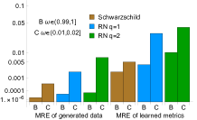
Figure 3: The performance of the DNN. (a) The curves are the target metrics and the markers are the results learned from the data A, which has a wide frequency range. (b) The right half of the bars represents the MRE of the metrics which are learned from the data with narrow ranges B and C. The left half represents the MRE of the wideband data, which are generated using the metrics learned from the narrowband.

Beyond Einstein-Maxwell.—Our DNN is not only applicable to the Einstein-Maxwell theory. In the SM, we demonstrate in general that the DNN can be applied to the Einstein-Maxwell-dilaton (EMD) theory with the typical potential and coupling of the dilaton Gubser0911 . The only nontrivial constraint is that the conformal dimension of the dilaton operator $\Delta_{\phi}$ should be less than 5/2. To be more specific, we further study a concrete EMD theory. It admits the analytical black hole solution with $\Delta_{\phi}=2$ and its holographic renormalization has been given in Kim1608 . This exemplifies our general argument explicitly. We also carry out the numerical experiments as before. It is found that the performance of the DNN for the EMD black hole is similar to that for the RN, see TABLE S.1. Note that at the zero-temperature limit, the EMD black hole becomes a special hyperscaling violating Lifshitz geometry with the asymptotic AdS. Moreover, here the metric components $g_{tt}(r)g_{rr}(r)\neq 1$. So what the DNN has learned is the joint factor

$$f(z)=\left.\frac{1}{r^{2}}\sqrt{\frac{g_{tt}(r)}{g_{rr}(r)}}\right|_{r=r_{h}/z},$$ (16)

as we will explain below.

Viscosity and entanglement.—A more general metric like the EMD black hole has two independent components $g_{tt}$ and $g_{rr}$. From Eq. (5), one can find that they appear in the form of the joint factor $g_{rr}/g_{tt}$. Therefore, without the constraint on the energy-momentum tensor for $g_{tt}g_{rr}=1$, the DNN still can be applied to learn the joint factor, but in general each of them cannot be learned separately from the shear response. Nevertheless, if there is another way to determine one component, the other can be obtained by the DNN. For example, there is evidence that the entanglement plays an important role in weaving the spacetime Maldacena0106 ; RT0603 ; Swingle0905 ; Raamsdonk1010 ; Susskind1306 . Among others, it has been shown that the holographic entanglement entropy $S(l)$ can be used to fix the bulk metric wherever the extremal surface reaches Bilson0807 , which can be described as

$$\left.r\sqrt{g_{rr}(r)}\right|_{r=r_{h}/z}=\frac{1}{2\pi^{2}L}z^{2}\partial_{z}\int_{z_{b}}^{z}\frac{z_{\ast}S(z_{\ast})}{\sqrt{z^{4}-z_{\ast}^{4}}}dz_{\ast},$$ (17)

where we have set the gravitational constant $16\pi G=1$ and $z_{\ast}$ is determined by $S^{\prime}(l)=8\pi L/z_{\ast}^{2}$. Note that $l$ and $L$ denote the finite width and the (regularized) infinite length of the rectangle on which the extremal surface is anchored RT0603 . Since the holographic entanglement entropy is only related to $g_{rr}$, it can complement to the shear viscosity to determine two metric components.

Conclusion and discussion.—Using a simple DL algorithm, we studied an inverse problem of AdS/CFT: Given the complex frequency-dependent shear viscosity of boundary field theories at finite temperatures, can the bulk metrics of black holes be extracted? We showed that Schwarzschild, RN, and EMD metrics can be learned by the DNN with high accuracy. The network architecture can be taken as a discretized representation of the holographic RG flow of the shear viscosity, hence supporting the underlying relationship among DL, RG, and gravity. We pointed out that our DNN is applicable to any strongly coupled field theory provided that: it is dual to the (3+1)-dimensional Einstein gravity minimally coupled with matter, it allows a homogeneous and isotropic black hole solution, the graviton mass in the wave equation vanishes, and the UV relation (7) holds. The extensions to the symmetry-breaking situations, the higher spacetime dimensions, and the modified theories of gravity should be worthwhile. Among others, we note that using the wave equation with the graviton mass which has been built up in Hartnoll1601 , one can construct the RG flow and the DNN where the graviton mass is encoded into new trainable weights. It is interesting to study whether the DNN can learn the metric and the mass simultaneously. In addition to various extensions, there are two open questions which should be mentioned. (i) Is there a better ansatz for the regularization term? Note that the regularization in this work is not to prevent overfitting as usual in machine learning. Instead, it is a guide to the minimum loss. We might need a deeper physical understanding of the regularization. (ii) How to reduce the discretized error at high frequencies and low temperatures sufficiently? Compared with directly increasing the number of layers, a more efficient method might be to apply the recently proposed DNN models of ordinary differential equations Chen1806 . We ultimately hope that our work could suggest a data-driven way to study holographic transports.

Moreover, we found that the complete black hole metric from IR to UV can be well learned from the data with narrow frequency ranges. We also checked that the performance of the DNN is hardly changed by randomly deleting several data points in our numerical experiments. These two facts indicate that the shear viscosity encodes the spacetime in a very different way from the entanglement entropy. The latter probes the deeper spacetime only by the $S(l)$ with a larger $l$, so any data point is necessary to reconstruct the spacetime. Perhaps we can describe the difference concisely as follows: the non-local observable (entanglement entropy) on the boundary probes the bulk spacetime locally, while the local observable (shear viscosity) probes it non-locally.

Furthermore, this non-locality leads to the excellent generalization ability of the DNN, which should be important in the application to the experimental data collected only in a part of the spectrum. Theoretically, from the perspective of machine learning, it usually implies that the data are highly structured. This structure is often important but obscure, due to the infamous black-box problem of machine learning. However, here the structure is nothing but the higher-dimensional black hole spacetime. This strong emergence might shed some light on the understanding of DL. Last but not least, the excellent generalization suggests that the strongly coupled field theories with gravity dual could exhibit another feature of the hologram in addition to encoding the higher dimension: The local (a small piece of the hologram) can reproduce the whole, see the schematic diagram FIG. (4).

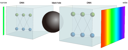
Figure 4: Schematic diagram: the DNN encodes the black hole spacetime, by which a wide spectrum of the field theory data can be generated from its narrow piece.

Acknowledgments.—We thank Koji Hashimoto for reading the draft and giving valuable comments. We also thank Matteo Baggioli, Yongcheng Ding, Wei-Jia Li, Tomi Ohtsuki, and Fu-Wen Shu for helpful discussions. SFW and XHG are supported by NSFC grants No. 11675097 and No. 11875184, respectively. YT is supported partially by NSFC grants No. 11975235 and No. 11675015. He is also supported by the “Strategic Priority Research Program of the Chinese Academy of Sciences” with Grant No. XDB23030000.

Supplementary material for
‘Deep learning black hole metrics from shear viscosity’

I Complex frequency-dependent shear viscosity

Compared to the real shear viscosity at the zero frequency limit, the study of the complex frequency-dependent counterpart is rare. So let’s begin from reviewing the Kubo formula of the complex frequency-dependent shear viscosity. In Read1207 , the Kubo formulas for the stress-stress response function at zero wavevector is derived from first principles. The approach given in Read1207 starts from a microscopic Hamiltonian and define the viscosity tensor as the linear response to a uniform external strain. In Wu2015 , an alternative field-theory approach is proposed, by which the Ward identity of viscosity coefficients in Read1207 is retrieved and extended. Here we will follow Wu2015 to give the definition of the complex frequency-dependent shear viscosity by the generating functional.

For a theorist, the viscosity can be measured by sending a gravitational wave through the system Son2007 . Suppose that a homogeneous and isotropic system lives in the two-dimensional flat space which is perturbed by a uniform gravitational wave. The response tensor $Y^{ijkl}$ can be defined by

$$\delta\langle T^{ij}(t)\rangle_{\mathrm{r}}=-\frac{1}{2}\int dt^{\prime}Y^{ijkl}(t-t^{\prime})\partial_{t^{\prime}}\delta g_{\mathrm{r}kl}(t^{\prime}).$$ (S.1)

Here the subscript $\mathrm{r}$ and the subscript $\mathrm{a}$ below indicate that we have invoked the closed time-path formalism to discuss the real-time response. The elastic modulus and the viscosity tensor can be further defined by separating the right hand of Eq. (S.1) into two parts,

$$\delta\langle T^{ij}(t)\rangle_{\mathrm{r}}=-\frac{1}{2}\int dt^{\prime}\lambda^{ijkl}(t-t^{\prime})\delta g_{\mathrm{r}kl}(t^{\prime})-\frac{1}{2}\int dt^{\prime}\eta^{ijkl}(t-t^{\prime})\partial_{t^{\prime}}\delta g_{\mathrm{r}kl}(t^{\prime}).$$ (S.2)

The stress tensor can be derived by the variation of the generating functional with respect to the metric

$$\langle T^{ij}(t)\rangle_{\mathrm{r}}=\frac{2}{\sqrt{g}}\frac{\delta W}{\delta g_{\mathrm{a}ij}(t)},$$ (S.3)

and the second variation leads to the retarded correlator

$$G_{\mathrm{ra}}^{ij,kl}(t)\equiv\frac{4\delta W}{\delta g_{\mathrm{a}ij}(t)\delta g_{\mathrm{r}kl}(0)}=\delta^{kl}\langle T^{ij}\rangle\delta(t)-\lambda^{ijkl}(t)-\partial_{t}\eta^{ijkl}(t).$$ (S.4)

The elastic modulus is the stress response up to the zeroth-order in time derivatives, which can be determined by the constitute relation of perfect fluids. In hydrodynamic expansion, one has

$$\delta\langle T^{ij}(t)\rangle_{\mathrm{r}}=-\left(P\delta^{ik}\delta^{jl}+\frac{1}{2}\delta^{ij}\delta^{kl}\kappa^{-1}\right)\delta g_{\mathrm{r}kl}(t),$$ (S.5)

where $P$ is the pressure and $\kappa^{-1}$ is the inverse compressibility. Then the elastic modulus can be given by

$$\lambda^{ijkl}(t)=\left[P\left(\delta^{ik}\delta^{jl}+\delta^{il}\delta^{jk}\right)+\delta^{ij}\delta^{kl}\kappa^{-1}\right]\delta(t).$$ (S.6)

The viscosity tensor can be decomposed as

$$\eta^{ijkl}(t)=\zeta(t)\delta^{ij}\delta^{kl}+\eta(t)\left(\delta^{ik}\delta^{jl}+\delta^{il}\delta^{jk}-\delta^{ij}\delta^{kl}\right)+\eta^{H}(t)\left(\delta^{jk}\epsilon^{il}-\delta^{il}\epsilon^{kj}\right).$$ (S.7)

The coefficients $\zeta,\eta,\eta^{H}$ denote the bulk, shear, and Hall viscosities, respectively. Substituting the last two equations into Eq. (S.4), one can obtain

$$G_{\mathrm{ra}}^{12,12}(t) = -\lambda^{1212}(t)-\partial_{t}\eta^{1212}(t)$$ (S.8)

$$= -P\delta(t)-\partial_{t}\eta(t).$$

In Fourier space, we have the Kubo formula of the shear viscosity

$$\eta(\omega)=\frac{G_{\mathrm{ra}}^{12,12}(\omega)+P}{i\omega}.$$ (S.9)

Note that this formula applies to the complex shear viscosity at all frequencies. In contrast, many literatures focus on the real part and the DC limit of the shear viscosity, so the pressure in Eq. (S.9) is often neglected.

II Holographic renormalization

We proceed to bridge the shear viscosity $\eta(\omega)$ to the shear response $\chi(\omega)$. The essential procedure is to carry out the holographic renormalization Henningson9806 . Consider that the bulk action includes the Einstein gravity and the minimally coupled matter

$$S_{\mathrm{bulk}}=\int d^{4}x\sqrt{-g}\left(R+6+L_{\mathrm{matter}}\right),$$ (S.10)

where we have set the AdS radius $L=1$ and the Newton constant $16\pi G_{N}=1$. Suppose that the background metric is homogeneous and isotropic along the field theory directions

$$ds^{2}=-g_{tt}(r)dt^{2}+g_{rr}(r)dr^{2}+g_{xx}(r)d\vec{x}^{2}.$$ (S.11)

Accordingly, the energy-momentum tensor can be written by

$$T_{\mu\nu}=\mathrm{diag}\left(T_{tt}(r),T_{rr}(r),T_{xx}(r),T_{xx}(r)\right).$$ (S.12)

Perturbing the Einstein equation on the background, the wave equation of the shear mode is derived as Hartnoll1601

$$\frac{1}{\sqrt{-g}}\partial_{r}(\sqrt{-g}g^{rr}\partial_{r}h)+g^{tt}\omega^{2}h=0,$$ (S.13)

where we have assumed that the square of the graviton mass $m^{2}=g^{xx}T_{xx}-\delta T_{xy}/\delta g_{xy}$ is vanishing. Without loss of generality, we will set $g_{xx}=r^{2}$ hereafter. We further require that the metric can be expanded near the AdS boundary, with the form

$$g_{tt} = r^{2}(1+\frac{a_{1}}{r}+\frac{a_{2}}{r^{2}}+\frac{a_{3}}{r^{3}}+\cdots),$$

$$g^{rr} = r^{2}(1+\frac{b_{1}}{r}+\frac{b_{2}}{r^{2}}+\frac{b_{3}}{r^{3}}+\cdots),$$ (S.14)

where $a_{i}$ and $b_{i}$ are some constants.

Near the boundary, the wave equation of the shear mode has the asymptotic solution

$$h=h^{(0)}+\frac{1}{r^{2}}h^{(2)}+\frac{1}{r^{3}}h^{(3)}+\cdots.$$ (S.15)

Here $h^{(0)}$ is the source, $h^{(2)}$ is fixed by $h^{(0)}$ as $h^{(2)}=h^{(0)}\omega^{2}/2$, and $h^{(3)}$ relies on $h^{(0)}$ and the incoming boundary condition on the horizon. In solving the asymptotic equation, one can find

$$\left(a_{1}+b_{1}\right)\omega^{2}h^{(0)}=0.$$ (S.16)

The situation $a_{1}=-b_{1}\neq 0$ is rare, if existed. So we focus on $a_{1}=-b_{1}=0$.

We write down the Gibbons-Hawking term and the counterterms

$$S_{\mathrm{GH}} = -2\int d^{3}x\sqrt{-\gamma}K,$$ (S.17)

$$S_{\mathrm{ct}} = \int d^{3}x\sqrt{-\gamma}\left(-4+R+L_{\mathrm{matter}}^{(1)}\right),$$ (S.18)

where $\gamma^{ab}$ is the induced metric, $K$ is the external curvature, and $L_{\mathrm{matter}}^{(1)}$ is contributed by the matter.

We expand the on-shell bulk action, the Gibbons-Hawking term and the counterterms to the quadratic order of the shear mode,

$$\left.S_{\mathrm{bulk}}+S_{\mathrm{GH}}+S_{\mathrm{ct}}\right|_{\mathrm{on-shell,\;quadratic}}$$ (S.19)

$$= \int d^{2}x\int_{-\infty}^{\infty}\frac{d\omega}{2\pi}\frac{1}{2}\left[\left(-\frac{r^{2}\omega^{2}}{\sqrt{g_{tt}}}+4r^{2}\sqrt{g_{tt}}-2r\sqrt{\frac{g_{tt}}{g_{rr}}}-\frac{r^{2}g_{tt}^{\prime}}{\sqrt{g_{tt}g_{rr}}}+L_{\mathrm{matter}}^{(2)}\right)\bar{h}h-r^{2}\sqrt{\frac{g_{tt}}{g_{rr}}}\bar{h}h^{\prime}\right],$$

where $\bar{h}$ has the argument $-\omega$ and $L_{\mathrm{matter}}^{(2)}$ denotes the matter contribution which may be divergent on the boundary.

Substituting the asymptotic solution (S.15) and the metric (S.14) into Eq. (S.19), we obtain the renormalized action:

$$S_{\mathrm{ren}}=\int d^{2}x\int_{-\infty}^{\infty}\frac{d\omega}{2\pi}\frac{1}{2}\left[(3a_{3}-2b_{3}+L_{\mathrm{matter}}^{(3)})\bar{h}^{(0)}h^{(0)}+3\bar{h}^{(0)}h^{(3)}\right],$$ (S.20)

where $L_{\mathrm{matter}}^{(3)}$ is contributed by the matter and it is finite.

Invoking the holographic dictionary, one can extract the retarded correlator from $S_{\mathrm{ren}}$:

$$G_{\mathrm{ra}}^{12,12}(\omega)=(3a_{3}-2b_{3}+L_{\mathrm{matter}}^{(3)})+3\frac{h^{(3)}}{h^{(0)}}.$$ (S.21)

Expand the response function near the boundary, which yields

$$\chi\equiv\frac{\Pi}{i\omega h}=-\frac{\sqrt{-g}g^{rr}\partial_{r}h}{i\omega h}=\left.\frac{3}{i\omega}\frac{h^{(3)}}{h^{(0)}}-i\omega r\right|_{r\rightarrow\infty}.$$ (S.22)

Then we have

$$G_{\mathrm{ra}}^{12,12}(\omega)=(3a_{3}-2b_{3}+L_{\mathrm{matter}}^{(3)})+i\omega\left(\chi+i\omega r\right)_{r\rightarrow\infty}.$$ (S.23)

Reading the pressure $P=-G_{\mathrm{ra}}^{12,12}(0)$ from Eq. (S.9) and the DC response $\chi(0)=r_{h}^{2}$ from Eq. (5) of the main text, we find

$$G_{\mathrm{ra}}^{12,12}(\omega)=-P+i\omega\left(\chi+i\omega r\right)_{r\rightarrow\infty}+L_{\mathrm{matter}}^{(3)}\left(\omega\right)-L_{\mathrm{matter}}^{(3)}\left(0\right).$$ (S.24)

Notice that given the Dirichlet boundary conditions as usual, $L_{\mathrm{matter}}^{(1)}$ should be an intrinsic scalar on the 2+1-dimensional boundary, which indicates that we can parameterize

$$L_{\mathrm{matter}}^{(3)}\left(\omega\right)-L_{\mathrm{matter}}^{(3)}\left(0\right)=\omega^{2}M,$$ (S.25)

where $M$ represents a finite real number.

Combining Eq. (S.24), Eq. (S.25) and Eq. (S.9), we obtain the relation between shear response and shear viscosity

$$\eta(\omega)=\left.\chi(\omega)+i\omega r\right|_{r\rightarrow\infty}-i\omega M.$$ (S.26)

Some remarks on the parameter $M$ are in order. First of all, for the Einstein-Maxwell theory, $M$ is equal to zero. Second, it is also vanishing for some other matter fields. We take the massive scalar field $\phi$ as an example, which is dominated by

$$L_{\mathrm{matter}}=-\frac{1}{2}g^{\mu\nu}\partial_{\mu}\phi\partial_{\nu}\phi-\frac{1}{2}m_{\phi}^{2}\phi^{2}.$$ (S.27)

It is dual to the relevant operator with the conformal dimension $\Delta_{\phi}=\frac{3}{2}+\sqrt{\frac{9}{4}+m_{\phi}^{2}}$ when $\Delta_{\phi}<3$. The scalar field yields two counterterms related to $\omega^{2}$, that is

$$L_{\mathrm{matter}}^{(1)}=\phi\nabla^{2}\phi+R\phi^{2},$$ (S.28)

where we have neglected two prefactors. When $\Delta_{\phi}<5/2$, these two terms do not contribute to $M$. Third, for the bottom-up holographic model, usually only the IR behavior of the metric is concerned. Instead, the holographic renormalization depends on the UV alone. Thus, one can assume that the target IR metric is embedded into a suitable UV background, by which $M=0$. In the main text, we focus on the UV-complete metrics with $M=0$ for simplicity. More generally, one can follow this philosophy. Thus, for a large class of strongly coupled theories with gravity dual, we have obtained

$$\eta(\omega)=\left.\chi(\omega)+i\omega r\right|_{r\rightarrow\infty}.$$ (S.29)

III Einstein-Maxwell-dilaton theory

We will illustrate that our DNN can be applied to the Einstein-Maxwell-dilaton (EMD) theory Gubser0911 . Consider the bulk action in a $d+1$-dimensional spacetime

$$S_{\mathrm{bulk}}=\int d^{d+1}x\sqrt{-g}\left[R-\frac{Z\left(\phi\right)}{4}F^{\mu\nu}F_{\mu\nu}-\frac{1}{2}\nabla_{\mu}\phi\nabla^{\mu}\phi-V\left(\phi\right)\right].$$ (S.30)

Here $V\left(\phi\right)$ is the potential of the dilaton and $Z\left(\phi\right)$ is the coupling between the dilaton and the gauge field. For any dilaton functions, the wave equation of the shear mode is same as Eq. (S.13). The dilaton functions should be constrained to accommodate a spacetime solution with asymptotically AdS. Typically, they can be expanded near the AdS boundary

$$Z\left(\phi\right) = 1+\cdots,$$

$$V\left(\phi\right) = -d(d-1)+\frac{1}{2}V_{2}\phi^{2}+\cdots,$$ (S.31)

where the ellipsis denotes the higher order terms of $\phi$. Using the gauge

$$ds^{2}=d\rho^{2}+\gamma_{ij}(\rho,x)dx^{i}dx^{j},\;A_{\rho}=0,$$ (S.32)

we further require the boundary conditions of the fields as Papadimitriou0505

$$\gamma_{ij}(\rho,x)\simeq e^{2\rho}\bar{\gamma}_{ij}(x),\;A_{i}(\rho,x)\simeq A_{i}(x),\;\phi(\rho,x)\simeq e^{-(d-\Delta_{\phi})\rho}\bar{\phi}(x),$$ (S.33)

where the conformal dimension is

$$\Delta_{\phi}=\frac{d}{2}+\sqrt{\frac{d^{2}}{4}+m_{\phi}^{2}}$$ (S.34)

with the mass square

$$m_{\phi}^{2}=\left.\frac{\partial^{2}}{\partial\phi^{2}}\left[V\left(\phi\right)+\frac{Z\left(\phi\right)}{4}F^{2}\right]\right|_{\phi=0}.$$ (S.35)

According to the holographic renormalization, especially the Hamilton-Jacobi approach HJ , one can build up the most general ansatz for the intrinsic counterterms on the boundary

$$S_{\mathrm{ct}}=-2\int d^{d}x\sqrt{-\gamma}U(\gamma^{ij},A_{i},\phi).$$ (S.36)

It can be organized in an expansion

$$U=U_{(0)}+U_{(2)}+\cdots+U_{(2\left\lfloor\frac{d}{2}\right\rfloor)},$$ (S.37)

where $U_{(2k)}$ contains $k$ inverse metrics and $\left\lfloor d/2\right\rfloor$ denotes the integer no more than $d/2$. Hereafter, we will focus on $d=3$ and $U=U_{(0)}+U_{(2)}$.

Keeping in mind the U(1) symmetry, one can find that the contribution of gauge fields starts from $U_{(4)}$. The dilaton may contribute to both $U_{(0)}$ and $U_{(2)}$. The leading terms of $U_{(2)}$ with the dilaton are $\phi\nabla^{2}\phi$ and $R\phi^{2}$. Thus, as analyzed in the previous section, we can set $\Delta_{\phi}<5/2$ to impose the vanishing of the matter parameter $M$.

We proceed to study a concrete EMD theory Gubser0911 . We specify the potential and the coupling as

$$Z\left(\phi\right)=\exp(\phi/\sqrt{3}),\;V\left(\phi\right)=-6\cosh(\phi/\sqrt{3}).$$ (S.38)

This theory allows an analytical black hole solution

$$ds^{2} = u^{2}f_{2}(u)\left(-f_{1}(u)dt^{2}+dx^{2}+dy^{2}\right)+\frac{1}{u^{2}f_{1}(u)f_{2}(u)}du^{2},$$ (S.39)

$$f_{1}(u) = 1-\frac{1}{\left(Q+u\right)^{3}}\left(m_{+}+Q^{3}\right),$$

$$f_{2}(u) = \left(1+\frac{Q}{u}\right)^{\frac{3}{2}},$$

associated with the profile of matter fields

$$A = \frac{\sqrt{3Q\left(m_{+}+Q^{3}\right)}}{Q+u_{+}}\frac{u-u_{+}}{Q+u}dt,$$ (S.40)

$$\phi(u) = \frac{\sqrt{3}}{2}\log\left(1+\frac{Q}{u}\right),$$ (S.41)

where $m_{+}$ and $Q$ are two independent parameters. Note that $m_{+}$ is related to the horizon radius $u_{+}$. Interestingly, when the black hole solution approaches extremality, it interpolates the asymptotic AdS on the UV and the conformal-to-AdS₂ geometry on the IR with the Lifshitz and hyperscaling violating exponents $z=\infty\$and $-\theta/z=1$.

Substituting the background solution into Eq. (S.34) and Eq. (S.35), we obtain the conformal dimension $\Delta_{\phi}=2$. Since it is less than $5/2$, we can infer the matter parameter $M=0$. Moreover, the holographic renormalization of this theory has been studied in Kim1608 . Consequently, we can double check $M=0$ by calculating the renormalized action explicitly. From Kim1608 , we read the counterterms

$$S_{\mathrm{ct}}=\int d^{3}x\sqrt{-\gamma}\left(-4+R+\frac{1}{3}\phi n^{u}\partial_{u}\phi-\frac{1}{6}\phi^{2}\right).$$ (S.42)

Note that we have selected the grand canonical ensemble and the mixed boundary condition of the dilaton has been imposed to be consistent with the thermodynamic first law. Here $n^{u}$ is the radial component of the outward unit vector normal to the boundary.

In order to use the formalism in the previous section, we need to change the coordinate $u\rightarrow r$, defined by

$$r=\sqrt{g_{uu}}=\left(1+\frac{Q}{u}\right)^{3/4}u.$$ (S.43)

The exact solution is lengthy. To be explicit, we expand Eq. (S.43) at small $Q$, which has the approximate solution

$$u=\frac{1}{4}(-3Q+\sqrt{3Q^{2}+16r^{2}}).$$ (S.44)

Then we read off

$$L_{\mathrm{matter}}^{(1)} = \frac{1}{3}\left[\phi n^{r}\partial_{r}\phi-\frac{1}{2}\phi^{2}\right],$$ (S.45)

$$L_{\mathrm{matter}}^{(2)} = \frac{1}{12}\left[\frac{1}{2}\sqrt{g_{tt}}r^{2}\phi^{2}-\frac{\sqrt{g_{tt}}}{\sqrt{g_{rr}}}r^{2}\phi\phi^{\prime}\right]\bar{h}h,$$ (S.46)

$$L_{\mathrm{matter}}^{(3)} = \frac{1}{16}Q^{3}\bar{h}h.$$ (S.47)

As expected, one can find

$$L_{\mathrm{matter}}^{(3)}\left(\omega\right)-L_{\mathrm{matter}}^{(3)}\left(0\right)=\omega^{2}M=0.\$$ (S.48)

Also, we have checked that $M$ is still zero for large $Q$.

Then we can carry out the numerical experiments. We set the horizon radius $u_{+}=1$ for convenience. The performance of the DNN for the EMD black hole is similar to that for the RN black holes.

IV Training scheme and report

For all numerical experiments in this paper, we implement the same training scheme. We train the network in two stages. First, the initial weights are randomly selected from $\left(0,2\right)$. The loss function is given by the sum of Eq. (12) and Eq. (13) of the main text. We will adopt the RMSProp optimizer RMSProp . Second, the initial weights of the DNN will be replaced by the trained weights of the first stage. The loss function is re-set as Eq. (12) of the main text without the regularization. Then the network will be trained again with the optimizer Adam Adam . After the training of each stage, one can read the loss, extract the weights, and calculate their error. It can be found that after the second stage of training, the performance of the DNN is usually improved. In particular, the loss (without regularizations) of the first stage can be reduced by several orders of magnitude. Moreover, turning the regularization factors in the first stage can improve the performance of the DNN in the second stage. With this in mind, we will scan the parameter space of regularization factors.

In two stages of training, we fix the batch size $c_{\mathrm{bs}}=512$, but the learning rate is changed even not once and selected by experience. The number of epoches in each stage is large enough so that the training will not stop until the validation loss is almost not reduced. The regularization factor $c_{3}$ is set as $15c_{1}$. We focus on turning the regularization factors $c_{1}$ and $c_{2}$ because the performance of the DNN is more sensitive to them than other hyperparameters. Initially, $c_{1}\$and $c_{2}$ are limited to some suitable ranges. Then we scan the two-dimensional parameter space. Considering the statistical fluctuation due to the randomized initialization of the network, we train $5$ times for each set of regularization factors Iten1807 . We gradually move and reduce the ranges of parameters. We also gradually reduce the step sizes. Thus, the scanning is concentrated around the $c_{1}$ and $c_{2}$ where the DNN produces smaller losses. We stop the scanning when the step sizes $\Delta c_{1}<10^{-5}$ and $\Delta c_{2}<0.01$.

We select the optimal regularization factors as the ones according to the minimum loss. We read the minimum loss and the trained weights of the network accordingly, and then calculate the MRE of the weights and the MRE of the wideband data generated by the weights learned from narrowband data. These quantities are considered as the final performance of the DNN. We simply refer them as the “minimum loss”, the “learned metric”, the “MRE of learned metrics”, and the “MRE of generated data”, respectively. They have been exhibited in FIG. 3 of the main text and in TABLE S.1.

Table S.1: Training reports of various numerical experiments. We have five target metrics and each of them is learned from three datasets: A $\omega\in(0,1]$, B $\omega\in(0.99,1]$, and C $\omega\in(0.01,0.02]$. We list two optimal regularization factors and three quantities which characterize the performance of the DNN.

Target	Data	Optimal $c_{1}$	Optimal $c_{2}$	Minimum loss	MRE of learned metrics	MRE of generated data
Schwarzschild	A	$1.20\times 10^{-3}$	$2.02$	$1\times 10^{-13}$	$1\times 10^{-3}$	/
Schwarzschild	B	$1.4\times 10^{-4}$	$1.52$	$6\times 10^{-13}$	$2\times 10^{-3}$	$5\times 10^{-6}$
Schwarzschild	C	$3.4\times 10^{-4}$	$1.49$	$1\times 10^{-14}$	$5\times 10^{-3}$	$4\times 10^{-4}$
RN q=1	A	$9\times 10^{-5}$	$2.00$	$1\times 10^{-13}$	$1\times 10^{-3}$	/
RN q=1	B	$2.6\times 10^{-4}$	$1.30$	$7\times 10^{-13}$	$4\times 10^{-3}$	$3\times 10^{-5}$
RN q=1	C	$1.1\times 10^{-4}$	$0.90$	$1\times 10^{-14}$	$3\times 10^{-2}$	$2\times 10^{-3}$
RN q=2	A	$7\times 10^{-5}$	$1.25$	$1\times 10^{-12}$	$7\times 10^{-4}$	/
RN q=2	B	$6\times 10^{-5}$	$1.15$	$2\times 10^{-11}$	$1\times 10^{-2}$	$5\times 10^{-5}$
RN q=2	C	$4.2\times 10^{-4}$	$0.50$	$2\times 10^{-14}$	$4\times 10^{-2}$	$7\times 10^{-3}$
EMD Q=1	A	$8.5\times 10^{-4}$	$1.85$	$2\times 10^{-13}$	$1\times 10^{-3}$	/
EMD Q=1	B	$2.2\times 10^{-4}$	$1.20$	$1\times 10^{-12}$	$6\times 10^{-3}$	$5\times 10^{-5}$
EMD Q=1	C	$2.6\times 10^{-4}$	$1.00$	$1\times 10^{-14}$	$1\times 10^{-2}$	$1\times 10^{-3}$
EMD Q=5	A	$2.5\times 10^{-4}$	$1.16$	$6\times 10^{-13}$	$6\times 10^{-4}$	/
EMD Q=5	B	$1.1\times 10^{-4}$	$0.85$	$2\times 10^{-12}$	$4\times 10^{-3}$	$2\times 10^{-5}$
EMD Q=5	C	$3.0\times 10^{-4}$	$0.40$	$2\times 10^{-14}$	$4\times 10^{-2}$	$7\times 10^{-3}$

References

- (1) K. G. Wilson and J. Kogut, Phys. Rep. 12, 75 (1974).
- (2) K. G. Wilson, Rev. Mod. Phys. 55, 583 (1983).
- (3) J. Polchinski, Nucl. Phys. B 231, 269 (1984).
- (4) L. P. Kadanoff, Physics Physique Fizika 2, 263 (1966).
- (5) T. J. Sejnowski, The Deep Learning Revolution, The MIT Press, 2018.
- (6) X. G. Wen, http://url.cn/5eKhBBP. (In Chinese)
- (7) P. Mehta and D. J. Schwab, arXiv:1410.3831.
- (8) C. Bény, arXiv:1301.3124.
- (9) S. Saremi and T. J. Sejnowski, PNAS 110, 3071 (2013).
- (10) A. Paul and S. Venkatasubramanian, arXiv:1412.6621.
- (11) S. Braddea and W. Bialek, J. Stat. Phys. 167, 462 (2017) arXiv:1610.09733.
- (12) D. Oprisa and P. Toth, arXiv:1705.11023.
- (13) S. Foreman, J. Giedt, Y. Meurice, and J. Unmuth-Yockey, EPJ. Web. Conf. 175, 11025 (2018) arXiv:1710.02079.
- (14) S. Iso, S. Shiba and S. Yokoo, Phys. Rev. E 97, 053304 (2018) arXiv:1801.07172
- (15) S. H. Li and L. Wang, Phys. Rev. Lett. 121, 260601 (2018) arXiv:1802.02840
- (16) H. W. Lin, M. Tegmark, and D. Rolnick, J. Stat. Phys. 168, 1223-1247 (2017) arXiv:1608.08225.
- (17) M. Koch-Janusz and Z. Ringel, Nature. Phys. 14, 578 (2018) arXiv:1704.06279; P. M. Lenggenhager, D. E. Gokmen, Z. Ringel, S. D. Huber, and M. Koch-Janusz, Phys. Rev. X 10, 011037 (2020) arXiv:1809.09632.
- (18) J. M. Maldacena, Adv. Theor. Math. Phys. 2, 231 (1998) arXiv:hep-th/9711200.
- (19) S. S. Gubser, I. R. Klebanov, and A. M. Polyakov, Phys. Lett. B 428, 105 (1998) arXiv:hep-th/9802109.
- (20) E. Witten, Adv. Theor. Math. Phys. 2, 253 (1998) arXiv:hep-th/9802150.
- (21) L. Susskind and E. Witten, arXiv:hep-th/9805114.
- (22) J. C. Bridgeman and C. T. Chubb, J. Phys. A: Math. Theor. 50, 223001 (2017) arXiv:1603.03039.
- (23) U. Schollwöck, Ann. Phys. 326, 96-192 (2011) arXiv:1008.3477.
- (24) G. Evenbly and G. Vidal, J. Stat. Phys. 145, 891 (2011) arXiv:1106.1082.
- (25) G. Vidal, Phys. Rev. Lett. 99, 220405 (2007) arXiv:cond-mat/0512165; G. Vidal, Phys. Rev. Lett. 101, 110501 (2008) arXiv:quant-ph/0610099; G. Evenbly and G. Vidal, Phys. Rev. B 79, 144108 (2009) arXiv:0707.1454.
- (26) W. C. Gan and F. W. Shu, Int. J. Mod. Phys. D 26, 1743020 (2017), arXiv:1705.05750.
- (27) Y.-Z. You, Z. Yang, and X.-L. Qi, Phys. Rev. B 97, 045153 (2018) arXiv:1709.01223.
- (28) K. Hashimoto, S. Sugishita, A. Tanaka, and A. Tomiya, Phys. Rev. D 98, 046019 (2018) arXiv:1802.08313.
- (29) K. Hashimoto, S. Sugishita, A. Tanaka, and A. Tomiya, Phys. Rev. D 98, 106014 (2018) arXiv:1809.10536.
- (30) K. Hashimoto, Phys. Rev. D 99, 106017 (2019) arXiv:1903.04951.
- (31) H. Y. Hu, S. H. Li, L. Wang, and Y. Z. You, arXiv:1903.00804
- (32) X. Han and S. A. Hartnoll, Phys. Rev. X 10, 011069 (2020) arXiv:1906.08781.
- (33) J. Tan and C. B. Chen, Int. J. Mod. Phys. D 28, 1950153 (2019) arXiv:1908.01470.
- (34) J. Zaanen, Y. W. Sun, and Y. Liu, Holographic duality in condensed matter physics, (CUP, 2015), Section 7.
- (35) P. K. Kovtun, D. T. Son and A. O. Starinets, Phys. Rev. Lett. 94, 111601 (2005) arXiv:hep-th/0405231.
- (36) T. Schaefer and D. Teaney, Rept. Prog. Phys. 72, 126001 (2009) arXiv:0904.3107.
- (37) N. Iqbal and Hong Liu, Phys. Rev. D 79, 025023 (2009) arXiv:0809.3808.
- (38) I. Bredberg, C. Keeler, V. Lysov, and A. Strominger, JHEP 1103, 141 (2011) arXiv:1006.1902.
- (39) K. S. Thorne, R. H. Price and D. A. Macdonald, Black holes: the membrane paradigm, Yale University Press, New Haven 1986.
- (40) M. K. Parikh and F. Wilczek, Phys. Rev. D 58, 064011 (1998) arXiv:gr-qc/9712077.
- (41) S. A. Hartnoll, D. M. Ramirez, and J. E. Santos, JHEP 1603, 170 (2016) arXiv:1601.02757.
- (42) D. Nickel and D. T. Son, New. J. Phys. 13, 075010 (2011) arXiv:1009.3094.
- (43) I. Heemskerk and J. Polchinski, JHEP 06, 031 (2011) arXiv:1010.1264.
- (44) T. Faulkner, H. Liu and M. Rangamani, JHEP 08, 051 (2011) arXiv:1010.4036.
- (45) B. Bradlyn, M. Goldstein, and N. Read, Phys. Rev. B 86, 245309 (2012) arXiv:1207.7021.
- (46) M. Geracie, D. T. Son, C. Wu, and S. F. Wu, Phys. Rev. D 91, 045030 (2015) arXiv:1407.1252.
- (47) M. Henningson and K. Skenderis, JHEP 07, 023 (1998) arXiv:hep-th/9806087; S. de Haro, S. N. Solodukhin, and K. Skenderis, Commun. Math. Phys. 217, 595 (2001) arXiv:hep-th/0002230; M. Bianchi, D. Z. Freedman, and K. Skenderis, Nucl. Phys. B 631, 159 (2002) arXiv:hep-th/0112119.
- (48) J. de Boer, E. Verlinde and H. Verlinde, JHEP 08, 003 (2000) arXiv:hep-th/9912012; D. Martelli and W. Mueck, Nucl. Phys. B 654, 248 (2003) arXiv:hep-th/0205061; J. Kalkkinen, D. Martelli, and W. Mueck, JHEP 0104, 036 (2001) arXiv:hep-th/0103111; I. Papadimitriou and K. Skenderis, IRMA Lect. Math. Theor. Phys. 8, 73 (2005) arXiv:hep-th/0404176; H. Elvang and M. Hadjiantonis, JHEP 06, 046 (2016) arXiv:1603.04485; F. Chen, S. F. Wu, and Y. X. Peng, JHEP 07, 072 (2019) arXiv:1903.02672.
- (49) T. Jacobson, Class. Quant. Grav. 24, 5717 (2007) arXiv:0707.3222.
- (50) T. Akutagawa, K. Hashimoto, and T. Sumimoto, arXiv:2005.02636.
- (51) T. Faulkner, H. Liu, J. McGreevy, and D. Vegh, Phys. Rev. D 83, 125002 (2011) arXiv:0907.2694.
- (52) M. Edalati, J. I. Jottar and R. G. Leigh, JHEP 1001, 18 (2010) arXiv:0910.0645.
- (53) T. Andrade, M. Baggioli, and O. Pujolàs, Phys. Rev. D 100, 106014 (2019) arXiv:1903.02859.
- (54) M. Baggioli, S. Grieninger, and H. Soltanpanahi, Phys. Rev. Lett. 124, 081601 (2020) arXiv:1910.06331.
- (55) J. M. Maldacena, JHEP 04, 021 (2003) arXiv:hep-th/0106112.
- (56) S. Ryu and T. Takayanagi, Phys. Rev. Lett. 96, 181602 (2006) arXiv:hep-th/0603001.
- (57) B. Swingle, Phys. Rev. D 86, 065007 (2012) arXiv:0905.1317.
- (58) M. Van Raamsdonk, Gen. Rel. Grav. 42, 2323 (2010) arXiv:1005.3035.
- (59) J. Maldacena and L. Susskind, Fortsch. Phys. 61, 781 (2013) arXiv:1306.0533.
- (60) S. S. Gubser and F. D. Rocha, Phys. Rev. D 81, 046001 (2010) arXiv:0911.2898; K. Goldstein, S. Kachru, S. Prakash and S. P. Trivedi, JHEP 1008, 078 (2010) arXiv:0911.3586; C. Charmousis, B. Gouteraux, B. S. Kim, E. Kiritsis and R. Meyer, JHEP 1011, 151 (2010) arXiv:1005.469.
- (61) B. S. Kim, JHEP 1611, 044 (2016) arXiv:1608.06252.
- (62) S. Bilson, JHEP 08, 073 (2008) arXiv:0807.3695; JHEP 02, 050 (2011) arXiv:1012.1812.
- (63) R. T. Q. Chen., Y. Rubanova, J. Bettencourt, and D. Duvenaud, NIPS’18: Proceedings of the 32nd International Conference on Neural Information Processing Systems 6572-6583 (2018) arXiv:1806.07366.
- (64) For example, see: C. Wang, H. Zhai, and Y. Z. You, arXiv:1901.11103.
- (65) J. Halverson and C. Long, arXiv:2001.00555.
- (66) D. T. Son, Viscosity, Black Holes, and Relativistic Heavy Ion Collisions, Physics/Applied Physics colloquium at Stanford University, 2007.
- (67) I. Papadimitriou and K. Skenderis, JHEP 0508, 004 (2005) arXiv:hep-th/0505190.
- (68) T. Tieleman and G. Hinton. Lecture 6.5—RmsProp: Divide the gradient by a running average of its recent magnitude. COURSERA: Neural Networks for Machine Learning, 2012.
- (69) D. Kingma and J. Ba: Adam: arXiv:1412.6980.
- (70) R. Iten, T. Metger, H. Wilming, L. D. Rio, and R. Renner, Phys. Rev. Lett. 124, 010508 (2020) arXiv:1807.10300.