Necessary and Sufficient Conditions for
Frequency-Based Kelly Optimal Portfolio

Abstract

In this paper, we consider a discrete-time portfolio with $m\geq 2$ assets optimization problem which includes the rebalancing frequency as an additional parameter in the maximization. The so-called Kelly Criterion is used as the performance metric; i.e., maximizing the expected logarithmic growth of a trader’s account, and the portfolio obtained is called the frequency-based Kelly optimal portfolio. The focal point of this paper is to extend upon the results of our previous work to obtain various optimality characterizations on the portfolio. To be more specific, using Kelly’s criterion in our frequency-based formulation, we first prove necessary and sufficient conditions for the frequency-based Kelly optimal portfolio. With the aid of these conditions, we then show several new optimality characterizations such as expected ratio optimality and asymptotic relative optimality, and a result which we call the Extended Dominant Asset Theorem. That is, we prove that the $i$th asset is dominant in the portfolio if and only if the Kelly optimal portfolio consists of that asset only. The word “extended” on the theorem comes from the fact that it was only a sufficiency result that was proved in our previous work. Hence, in this paper, we improve it to involve a proof of the necessity part. In addition, the trader’s survivability issue (no bankruptcy consideration) is also studied in detail in our frequency-based trading framework. Finally, to bridge the theory and practice, we propose a simple trading algorithm using the notion called dominant asset condition to decide when should one triggers a trade. The corresponding trading performance using historical price data is reported as supporting evidence.

I Introduction

The takeoff point for this paper is the classical Kelly trading problem [1, 2, 5, 4, 3], which calls for maximizing the Expected Logarithmic Growth (ELG) of a trader’s account. To be more specific, the problem is often formulated by a sequence of trades with independent and identically distributed (i.i.d.) returns with known probability distribution. The trader’s objective is to specify a fraction $K$ of its account value at each stage seeking to maximize the ELG at the terminal stage. While many of the existing papers contributed on the Kelly’s problem and its application to stock trading; e.g., see [2, 18, 17, 3, 19, 5, 4], the effects of rebalancing frequency is still not heavily considered into the existing literature.

Some initial results along these lines regarding rebalancing frequency effects can be found in [14, 15, 16] and our most recent work in [9, 10, 11]. Indeed, in [14], a portfolio optimization with returns following a continuous geometric Brownian motion was considered. However, only two extreme cases: High-frequency trading and buy and hold were emphasized in their results. On the other hand, in [15] and [16], a portfolio optimization was considered with the constant gain $K$ selected without regard for the frequency with which the portfolio rebalancing is done. Subsequently, when this same gain $K$ is used to find an optimal rebalancing period, the resulting levels of ELG are arguably suboptimal.

In contrast to [14] and [15], our formulation to follow, achieved by adopting our previous work published in [9] and [10], considers full range of rebalancing frequencies and both the probability distribution of the returns and the time interval between rebalances are arbitrary. That is, we deal with what we view to be a more appropriate frequency-based Kelly trading formulation and seek an optimal portfolio which depends on the rebalancing frequency.

I-A Idea of Frequency-Based Formulation

Specifically, within this frequency-based trading context, we let $\Delta t$ be the time between trade updates and $n\geq 1$ be the number of steps between rebalancings. Then the frequency is $f:=1/(n\Delta t)$. In the sequel, we may call the quantity $n$ to be the rebalancing period. Now, letting $V(k)$ denote the trader’s account value at stage $k$, the trader invests $KV(0)$ with $K\geq 0$ at stage $k=0$ and waits $n\geq 1$ steps before updating the trade size. After each trade, the broker takes its share and the balance of the money is left to “ride” with resulting profits or losses viewed as “unrealized” until stage $n$ is reached. When $n$ is small, this is viewed as the high-frequency case, and when $n$ is large, one use the term “buy and hold”.

I-B Plan for the Remainder of the Paper

In Section II, we first recall our frequency-based formulation considered in [9] and [10]. Then, in Section III, based on the formulation, we offer our main result which gives necessary and sufficient conditions for the frequency-based optimal Kelly portfolio. In addition, several technical results regarding the various optimality conditions are also provided; e.g., extended dominant asset theorem, the expected ratio optimality, and asymptotic relative optimality are proved. In Section IV, we propose a simple trading algorithm which uses the idea of extended dominant asset theorem to determine when should one trigger a trade on an underlying asset or not. Several back-testing simulations using historical prices are provided to support the trading performance of the algorithm. In Section V, a concluding remark is provided. Finally, in Appendix, we also address an important issue regarding survivability (no-bankruptcy).

II Problem Formulation

To study the effect of rebalancing frequency in portfolio optimization problems, as seen in Section I, let $n\geq 1$ being the number of steps between rebalancings. For $k=0,1,\dots,$ we consider a trader who is forming a portfolio consisting of $m\geq 2$ assets and assume that at least one of them is riskless with nonnegative rate of return $r\geq 0.$ That is, if an asset is riskless, its return is deterministic and is treated as a degenerate random variable with value $r$ for all $k$ with probability one. Alternatively, if Asset $i$ is a stock whose price at time $k$ is $S_{i}(k)>0$, then its return is

$$X_{i}(k)=\frac{S_{i}(k+1)-S_{i}(k)}{S_{i}(k)}.$$

In the sequel, for stocks, we assume that the return vectors $X(k):=\left[X_{1}(k)\,X_{2}(k)\,\cdots\,X_{m}(k)\right]^{T}$ have a known distribution and have components $X_{i}(\cdot)$ which can be arbitrarily correlated. We also assume that these vectors are i.i.d. with components satisfying $X_{\min,i}\leq X_{i}(k)\leq X_{\max,i}$ with known bounds above and with $X_{\max,i}$ being finite and $X_{\min,i}>-1$. The latter constraint on $X_{\min,i}$ means that the loss per time step is limited to less than $100\%$ and the price of a stock cannot drop to zero.

II-A Feedback Control Perspectives

Consistent with the literature [6, 12, 9, 10, 7, 8, 11], we bring the control-theoretic point of view into our problem formulation. That is, the system output at stage $k$ is taken to be the trader’s account value $V(k)$ and the $i$th feedback gain $0\leq K_{i}\leq 1$ represents the fraction of the account allocated to the $i$th asset for $i=1,\dots,m$. Said another way, the $i$th controller is a linear feedback of the form $I_{i}(k)=K_{i}V(k).$ Since $K_{i}\geq 0$, the trader is going long. In view of the above and recalling that there is at least one riskless asset available, without loss of generality, we consider the unit simplex constraint

$$K\in{\mathcal{K}}:=\left\{K\in\mathbb{R}^{m}:K_{i}\geq 0\text{ for all $i$},\;\sum_{i=1}^{m}K_{i}=1\right\}$$

which is classical in finance; e.g., see [17, 2, 10]. That is, with $K\in\mathcal{K}$, we have a guarantee that 100% of the account is invested. Moreover, we claim that the constraint set $\mathcal{K}$ assures trader’s survivability; i.e., no bankruptcy is assured; see Appendix for a proof of this important property.

II-B Frequency-Dependent Dynamics and Feedback Setting

Letting $n\geq 1$ be the number of steps between rebalancings, at time $k=0$, the trader begins with initial investment control

$$u(0)=\sum_{i=1}^{m}K_{i}V(0)$$

and waits $n$ steps in the spirit of buy and hold. Then, when $k=n$, the investment control is updated to be $u(n)=\sum_{i=1}^{m}K_{i}V(n).$ Now, to study the performance which is dependent on rebalancing frequency, for $i=1,2,\ldots,m$, we use the compound returns

$$\mathcal{X}_{n,i}:=\prod_{k=0}^{n-1}(1+X_{i}(k))-1$$

which are readily seen to satisfy $\mathcal{X}_{n,i}>-1$ for all $n\geq 1$ and we work with the random vector $\mathcal{X}_{n}$ having $i$th component $\mathcal{X}_{n,i}$. Then, for an initial account value $V(0)>0$ and rebalancing period $n\geq 1$, the corresponding account value at stage $n$ is described by the stochastic recursion

$$V(n)=(1+K^{T}\mathcal{X}_{n})V(0).$$

In the sequel, we may sometimes write $V(n,K)$ to emphasize the dependence on the feedback gain $K$.

II-C Frequency-Dependent Optimization Problem

Consistent with our prior work in [9] and [10], for any rebalancing period $n\geq 1$, we study the problem of maximizing the expected logarithmic growth

$${g_{n}}(K) :=\frac{1}{n}\mathbb{E}\left[\log\frac{V(n,K)}{V(0)}\right]$$

$$=\frac{1}{n}\mathbb{E}\left[{\log(1+{K^{T}}{\mathcal{X}_{n}})}\right]$$

and we use $g_{n}^{*}$ to denote the associated optimal expected logarithmic growth. It is readily verified that $g_{n}(K)$ is concave in $K$. Furthermore, any vector $K^{*}\in\mathcal{K}\subset\mathbb{R}^{m}$ satisfying $g_{n}(K^{*})=g_{n}^{*}$ is called a Kelly optimal feedback gain. The portfolio which uses the Kelly optimal feedback gain is called frequency-based Kelly optimal portfolio.

III Results On Optimality

In this section, we provide necessary and sufficient conditions which characterize the frequency-based Kelly optimal portfolio.

Theorem 3.1 (Necessity and Sufficiency):

The feedback gain $K^{*}$ is optimal to the frequency-dependent optimization problem described in Section II if and only if for $i=1,2,\dots,m$,

$$\mathbb{E}\left[\frac{1+\mathcal{X}_{n,i}}{1+{K^{*}}^{T}\mathcal{X}_{n}}\right]=1,\;\;\;\text{ if }K_{i}^{*}>0$$

$$\mathbb{E}\left[\frac{1+\mathcal{X}_{n,i}}{1+{K^{*}}^{T}\mathcal{X}_{n}}\right]\leq 1,\;\;\;\text{ if }K_{i}^{*}=0.$$

Proof.

To prove necessity, define $\mathcal{R}_{n}:=\mathcal{X}_{n}+\bf{1}$ representing the total return with $i$th component $\mathcal{R}_{n,i}=\mathcal{X}_{n,i}+1$ and ${\bf 1}:=[1\;1\;\cdots\;1]^{T}\in\mathbb{R}^{m}$. We now consider the frequency-dependent optimization problem as an equivalent constrained convex minimization problem as follows:

$$\max_{K}-\mathbb{E}[\log K^{T}\mathcal{R}_{n}]$$

subject to

$$\hskip 14.22636ptK^{T}{\bf 1}-1=0;$$

$$\hskip 14.22636pt-K^{T}e_{i}\leq 0,\;\;\;i=1,2,...,m$$

where $e_{i}$ is unit vector having $1$ at $i$th component. Then the Karush-Kuhn-Tucker Conditions, see e.g., [13], tell us that if $K^{*}$ is a local maximum then there is a scalar $\lambda\in\mathbb{R}^{1}$ and a vector $\mu\in\mathbb{R}^{m}$ with component $\mu_{j}\geq 0$ such that

$$\nabla(-\mathbb{E}[\log{K^{*}}^{T}\mathcal{R}_{n}])+\lambda{\bf 1}-\sum_{i=1}^{m}\mu_{i}e_{i}=\textbf{0}$$

with $\textbf{0}\in\mathbb{R}^{m}$ being zero vector and $\mu_{j}{K^{*}}^{T}e_{j}=0$ for $j=1,2,\dots,m$. This implies that for $j=1,\dots,m$, we have $\mu_{j}{K_{j}^{*}}=0$ and

$$-\mathbb{E}\left[\frac{\mathcal{R}_{n,j}}{{K^{*}}^{T}\mathcal{R}_{n}}\right]+\lambda-\mu_{j}=0.$$ (1)

We note here that the interchanging of differentiation and expectation is justifiable since $\mathcal{X}_{n,i}$ is bounded. Now we take a weighted sum of equation (1); i.e.,

$$\sum_{j=1}^{m}K_{j}^{*}\left(-\mathbb{E}\left[\frac{\mathcal{R}_{n,j}}{{K^{*}}^{T}\mathcal{R}_{n}}\right]+\lambda-\mu_{j}\right)=0$$

which leads to

$$-\sum_{j=1}^{m}K_{j}^{*}\mathbb{E}\left[\frac{\mathcal{R}_{n,j}}{{K^{*}}^{T}\mathcal{R}_{n}}\right]+\sum_{j=1}^{m}K_{j}^{*}\lambda-\sum_{j=1}^{m}K_{j}^{*}\mu_{j}=0.$$

Using the facts that $\mu_{j}K_{j}^{*}=0$ for all $j$ and $\sum_{j=1}^{m}K_{j}^{*}=1$, we have

$$-\sum_{j=1}^{m}K_{j}^{*}\mathbb{E}\left[\frac{\mathcal{R}_{n,j}}{{K^{*}}^{T}\mathcal{R}_{n}}\right]+1\cdot\lambda+0=0.$$ (2)

Note that

$$\sum_{j=1}^{m}K_{j}^{*}\mathbb{E}\left[\frac{\mathcal{R}_{n,j}}{{K^{*}}^{T}\mathcal{R}_{n}}\right] =\mathbb{E}\left[\frac{{K^{*}}^{T}\mathcal{R}_{n}}{{K^{*}}^{T}\mathcal{R}_{n}}\right]=1.$$

Thus, substituting the result above back into equation (2), we obtain $\lambda=1$. This tells us that for $j=1,\dots,m$,

$$-\mathbb{E}\left[\frac{\mathcal{R}_{n,j}}{{K^{*}}^{T}\mathcal{R}_{n}}\right]+1-\mu_{j}=0$$

and $\mu_{j}{K_{j}^{*}}=0.$ Thus, to sum up, if $K_{j}^{*}>0$, implies that $\mu_{j}=0$ and

$$\mathbb{E}\left[\frac{\mathcal{R}_{n,j}}{{K^{*}}^{T}\mathcal{R}_{n}}\right]=1.$$

If $K_{j}^{*}=0,$ implies that $\mu_{j}\geq 0$ implies that

$$\mathbb{E}\left[\frac{\mathcal{R}_{n,j}}{{K^{*}}^{T}\mathcal{R}_{n}}\right]\leq 1.$$

Now, transforming the $\mathcal{R}_{n}$ back to $\mathcal{X}_{n}$ by $\mathcal{R}_{n}=\mathcal{X}_{n}+1$ and using the fact that $\sum_{i=1}^{m}K_{i}^{*}=1$ again, we obtain the desired conditions. Finally, by concavity of $\mathbb{E}[\log K^{T}\mathcal{R}_{n}]$, the conditions above are also sufficient. ∎

Remarks: It is interesting to note that if $n=1$, then Theorem 3.1 reduces to the classical result in classical Kelly theory; see [2, Theorem 16.2.1]. Additionally, Theorem 3.1 is also closely related to the Dominant Asset Theorem given in our prior work [10]. For the sake of completeness, we recall the statement of the theorem as follows: Given a collection of $m\geq 2$ assets, if Asset $j$ is dominant; i.e., Asset $j$ satisfies

$$\mathbb{E}\left[\frac{1+X_{i}(0)}{1+X_{j}(0)}\right]\leq 1$$

for every other asset $i\neq j$, then $K^{*}=e_{j}.$ Thus, $K_{i}^{*}=0$ for $i\neq j.$ In fact, this result can be viewed as a special case of Theorem 3.1. It should be also noted that the Dominant Asset Theorem is about sufficiency on optimal $K^{*}$— not necessity. Fortunately, with the aids of Theorem 3.1, we are now able to prove the missing part on necessity of Dominant Asset Theorem. This is summarized in the next theorem to follow.

Theorem 3.2 (Extended Dominant Asset Theorem):

The optimal Kelly feedback gain $K^{*}=e_{j}$ if and only if

$$\mathbb{E}\bigg{[}\frac{1+X_{i}(0)}{1+X_{j}(0)}\bigg{]}\leq 1.$$

Proof.

The sufficiency is proved in our prior work in [10, Dominant Asset Theorem]. Hence, for the sake of brevity, we only provide a proof of necessity here. Assuming that $K^{*}=e_{j}$, we must show the desired inequality holds. Applying Theorem 3.1, it follows that for $i\neq j,$ $K_{i}^{*}=0$ and

$$\mathbb{E}\left[\frac{1+\mathcal{X}_{n,i}}{1+{K^{*}}^{T}\mathcal{X}_{n,j}}\right]=\mathbb{E}\left[\frac{1+\mathcal{X}_{n,i}}{1+\mathcal{X}_{n,j}}\right]\leq 1.$$

Using the definition of $\mathcal{X}_{n,i}=\prod_{k=0}^{n-1}(1+X_{i}(k)))-1$, the equality above indeed implies that

$$\mathbb{E}\left[\prod_{k=0}^{n-1}\frac{1+X_{i}(k)}{1+X_{j}(k)}\right]\leq 1.$$

Since $X_{i}(k)$ are i.i.d., in $k$, we have

$$\left(\mathbb{E}\left[\frac{1+X_{i}(0)}{1+X_{j}(0)}\right]\right)^{n}\leq 1.$$ (3)

Note that $X_{i}(0)>-1$ for all $i=1,2,\dots,m$, it follows that the ratio

$$\frac{1+X_{i}(0)}{1+X_{j}(0)}>0$$

with probability one; hence its expected value is also strictly positive. Thus, in combination with inequality (3), we conclude

$$\mathbb{E}\left[\frac{1+X_{i}(0)}{1+X_{j}(0)}\right]\leq 1.\qed$$

Remark: When the condition

$$\mathbb{E}\bigg{[}\frac{1+X_{i}(0)}{1+X_{j}(0)}\bigg{]}\leq 1$$ (4)

the Extended Dominant Asset Theorem 3.2 tells us to invest all available funds on the $j$th asset. In the sequel, the inequality (4) is called the dominant asset condition. As seen later in Section IV, this condition allows us to construct a simple algorithm which may be useful for practical stock trading.

In the rest of this section, some other new optimality results are provided.

Lemma 3.3 (Expected Ratio Optimality):

Let $K^{*}$ be the frequency-based optimal Kelly feedback gain. Then

$$\mathbb{E}\bigg{[}\frac{1+{K}^{T}\mathcal{X}_{n}}{1+{K^{*}}^{T}\mathcal{X}_{n}}\bigg{]}\leq 1$$

for any $K$. In addition, we have

$$\mathbb{E}\bigg{[}\log\frac{1+K^{T}\mathcal{X}_{n}}{1+{K^{*}}^{T}\mathcal{X}_{n}}\bigg{]}\leq 0$$

for any $K$.

Proof.

Let $K$ be given. From Theorem 3.1, it follows that for a Kelly optimal feedback gain $K^{*}$, we have

$$\mathbb{E}\bigg{[}\frac{1+X_{n,i}}{1+{K^{*}}^{T}\mathcal{X}_{n}}\bigg{]}\leq 1$$

for all $i=1,\dots,m$. Multiplying this inequality by $K_{i}$ and summing over $i$, we obtain

$$\sum_{i=1}^{m}K_{i}\mathbb{E}\bigg{[}\frac{1+X_{n,i}}{1+{K^{*}}^{T}\mathcal{X}_{n}}\bigg{]}\leq\sum_{i=1}^{m}K_{i}=1$$

which is equivalent to

$$\mathbb{E}\bigg{[}\frac{1+{K}^{T}\mathcal{X}_{n}}{1+{K^{*}}^{T}\mathcal{X}_{n}}\bigg{]}\leq 1.$$

To complete the proof, we invoke Jensen’s inequality on the quantity $\mathbb{E}\left[\log\frac{1+K^{T}\mathcal{X}_{n}}{1+{K^{*}}^{T}\mathcal{X}_{n}}\right]$ and observe that

$$\mathbb{E}\bigg{[}\log\frac{1+K^{T}\mathcal{X}_{n}}{1+{K^{*}}^{T}\mathcal{X}_{n}}\bigg{]} \leq\log\mathbb{E}\bigg{[}\frac{1+K^{T}\mathcal{X}_{n}}{1+{K^{*}}^{T}\mathcal{X}_{n}}\bigg{]}$$

$$\leq\log 1=0.$$

Hence, the proof is complete. ∎

Remark: Lemma 3.3 above tell us that the frequency-based Kelly optimal portfolio also maximizes the expected relative wealth $\mathbb{E}[\frac{1+K^{T}\mathcal{X}_{n}}{1+{K^{*}}^{T}\mathcal{X}_{n}}]$. In addition, we note that the for any $K$,

$$1+K^{T}\mathcal{X}_{n} =1+\sum_{i=1}^{m}K_{i}\mathcal{X}_{n,i}$$

$$\geq 1+\min_{j}\mathcal{X}_{\min,j}\sum_{i=1}^{m}K_{i}$$

$$>0.$$

Hence, the ratio $\frac{1+K^{T}\mathcal{X}_{n}}{1+{K^{*}}^{T}\mathcal{X}_{n}}>0$. Now using the Markov inequality, the condition

$$\mathbb{E}\bigg{[}\frac{1+K^{T}\mathcal{X}_{n}}{1+{K^{*}}^{T}\mathcal{X}_{n}}\bigg{]}\leq 1$$

for any $K$ implies that

$$P\left(\frac{1+K^{T}\mathcal{X}_{n}}{1+{K^{*}}^{T}\mathcal{X}_{n}}>c\right)\leq\frac{1}{c}$$

for any $c>0.$ The following lemma indicates a stronger result on the asymptotic relative optimality of $K^{*}$.

Lemma 3.4 (Asymptotic Relative Optimality):

The optimal feedback vector $K^{*}$ is such that

$$\limsup_{n\to\infty}\frac{1}{n}\log\frac{1+K^{T}\mathcal{X}_{n}}{1+{K^{*}}^{T}\mathcal{X}_{n}}\leq 0$$

with probability one.

Proof.

The idea of the proof is very similar to the one presented in [2, Theorem 16.3.1]. However, for the sake of completeness, we provide our own proof here. Recalling Lemma 3.3, we have

$$\mathbb{E}\bigg{[}\frac{1+K^{T}\mathcal{X}_{n}}{1+{K^{*}}^{T}\mathcal{X}_{n}}\bigg{]}\leq 1$$

and Markov inequality tell us that

$$P\left(\frac{1+K^{T}\mathcal{X}_{n}}{1+{K^{*}}^{T}\mathcal{X}_{n}}>c_{n}\right)\leq\frac{1}{c_{n}}$$

for any $c_{n}>0.$ Hence,

$$P\left(\frac{1}{n}\log\frac{1+K^{T}\mathcal{X}_{n}}{1+{K^{*}}^{T}\mathcal{X}_{n}}>\frac{1}{n}\log c_{n}\right)\leq\frac{1}{c_{n}}.$$

Take $c_{n}:=n^{2}$ and summing all $n$, we have

$$\sum_{n=1}^{\infty}P\left(\frac{1}{n}\log\frac{1+K^{T}\mathcal{X}_{n}}{1+{K^{*}}^{T}\mathcal{X}_{n}}>\frac{2\log n}{n}\right)\leq\sum_{n=1}^{\infty}\frac{1}{n^{2}}<\infty.$$

Therefore, applying the Borel-Cantelli Lemma; e.g., see [20], it leads to

$$P\left(\frac{1}{n}\log\frac{1+K^{T}\mathcal{X}_{n}}{1+{K^{*}}^{T}\mathcal{X}_{n}}>\frac{2\log n}{n}\,\,\text{infinitely often}\right)=0.$$

Thus, there exists $N>0$ such that for all $n\geq N$, we have

$$\frac{1}{n}\log\frac{1+K^{T}\mathcal{X}_{n}}{1+{K^{*}}^{T}\mathcal{X}_{n}}\leq\frac{2\log n}{n}.$$

It follows that

$$\limsup_{n\to\infty}\frac{1}{n}\log\frac{1+K^{T}\mathcal{X}_{n}}{1+{K^{*}}^{T}\mathcal{X}_{n}}\leq 0$$

with probability one. ∎

Remark: Note that for $n\geq 1$, $V(n)=(1+K^{T}\mathcal{X}_{n})V(0)$, thus, Lemma 3.4 implies that

$$\limsup_{n\to\infty}\frac{1}{n}\log\frac{V(n)}{V^{*}(n)}\leq 0$$

with probability one where $V^{*}(n)=(1+{K^{*}}^{T}\mathcal{X}_{n})V(0)$.

IV Dominant Ratio Trading Algorithm

Besides the theoretical interests, as mentioned in Section III, we view that Theorem 3.1 and Extended Dominate Asset Theorem 3.2 may be useful to design an algorithm for practical stock trading. The main idea is to take advantage of the Dominant Asset Condition stated in Theorem 3.2; i.e.,

$$\mathbb{E}\left[\frac{1+X_{i}(k)}{1+X_{j}(k)}\right]\leq 1,$$

if it holds, then we set $K_{j}^{*}=1$; otherwise, $K_{j}^{*}=0.$

IV-A Bridging Theory and Practice

To implement the idea described above, we proceed as follows: Using $s_{i}(k)$ to denote the $k$th daily realized prices for the $i$th stock, we calculate the associated realized return, call it $x_{i}(k)$, where

$$x_{i}(k):=\frac{s_{i}(k+1)-s_{i}(k)}{s_{i}(k)}$$

for $i=1,2,\dots,m$. It should be noted that, in practice, the realized returns $x_{i}(k)$ are often nonstationary. Hence, when testing the dominant asset condition, we work with a sliding window consisting of the most recent $M$ trading steps. That is, we estimate the expected ratio in the Dominant Asset Condition by

$$R_{ij}(k):=\frac{1}{M}\sum_{\ell=0}^{M-1}\frac{1+x_{i}(k-\ell)}{1+x_{j}(k-\ell)}.$$

Then, if $R_{ij}\leq 1$ for all $i\neq j$, we set $K_{j}^{*}(k)=1$; otherwise, we set $K_{j}^{*}(k)=0.$ We call the procedure above the Dominant Ratio Trading Algorithm. An illustrative example using historical prices data is provided in the next subsection to follow.

IV-B Illustrative Example Via Back-Testing

Consider a one-year long portfolio consisting of three assets with duration from February 14, 2019 to February 14, 2020: Vanguard Total World Stock Index Fund ETF Shares (Ticker: VT), Vanguard Total Bond Market Index Fund ETF Shares (Ticker: BND), and Vanguard Total World Bond EFT (Ticker: BNDX) where the price trajectories are shown in Figure 1.

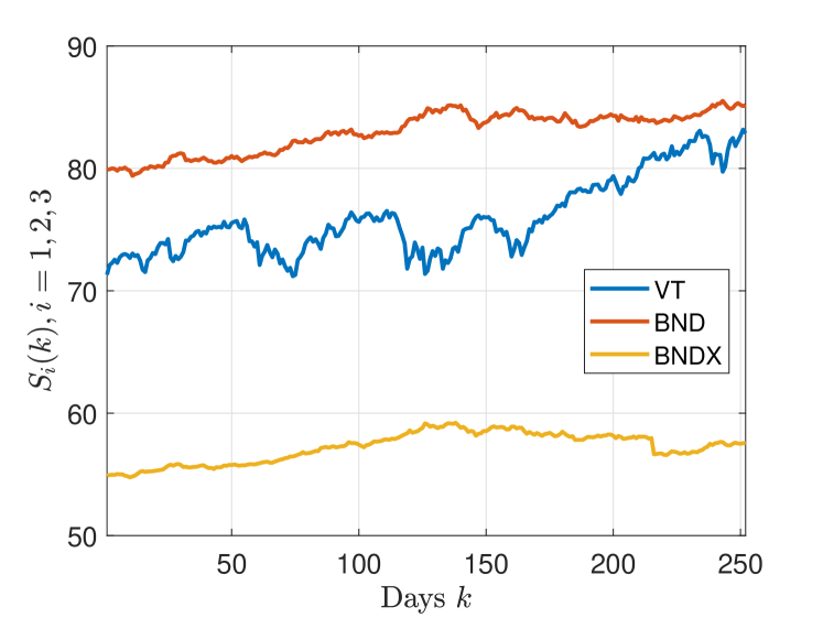
Figure 1: Daily Closing Stock Prices $S_{i}(k),i=1,2,3$ for VT, BND, and BNDX, respectively.

Begin with initial account value $V(0)=\$1$, we implement the algorithm described above using a window size $M=20$ days. That is, the initial trade is triggered after receiving the first twenty daily prices data. We ran MATLAB script and plot a typical trading performance in terms of the trajectory of account value $V(k)$, which is shown in Figure 2. In Figure 2, we find that the account value obtained by Dominant Ratio Trading Algorithm is increasing from $V(0)=1$ to $V(252)\approx 1.23$, which yields a returns about $23\%$ and is obviously higher than the account value obtained by standard buy and hold strategy. We also reported the corresponding trading signal $K_{i}(k)$ for $i=1,2,3$ in Figure 3 where a flavor of bang-bang control is seen. To close this section, we also tested various sliding window sizes using equally-spaced $M=1,5,15,\dots,60$ with increment $5$ between elements and we seen that the algorithm produces similar trading performance to the one seen in Figure 2. This example provides a potential for bridging the theory and practice in stock trading. Further developments along this line might be fruitful to pursue as a direction of future research. For example, an initial computational complexity analysis and trading with various stocks may be of the next interests to pursue.

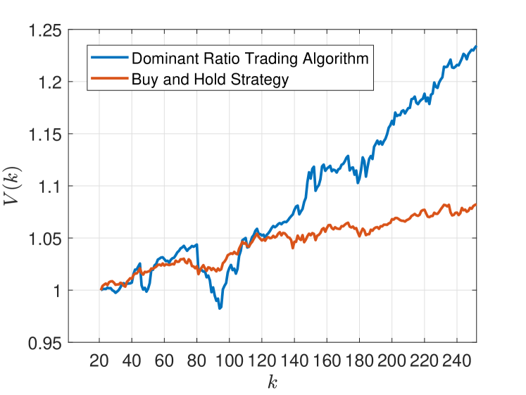
Figure 2: Trading Performance Comparison: Dominant Ratio Trading Algorithm with $M=20$ versus Buy and Hold strategy.

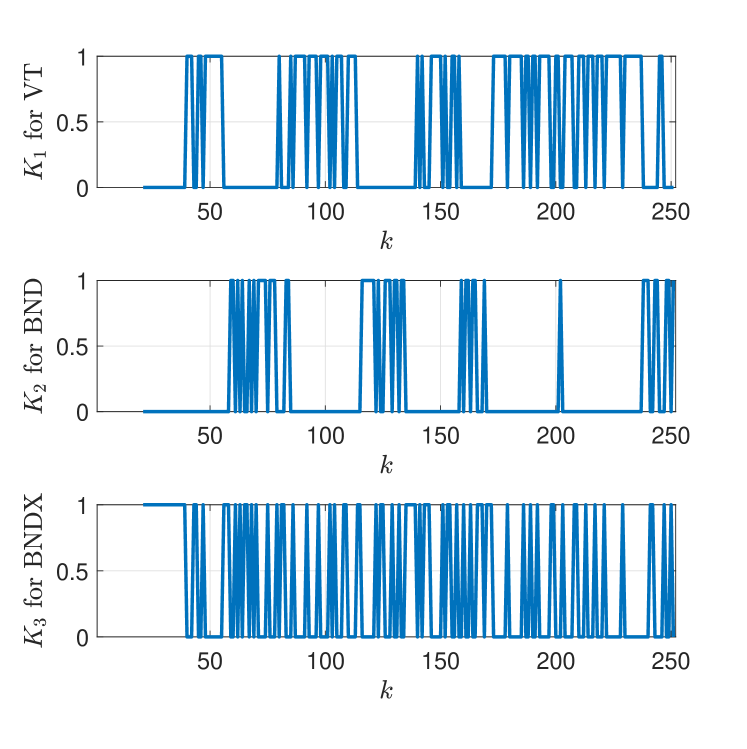
Figure 3: Feedback Gains $K_{i}(k)$ with $i=1,2,3$ for VT, BND, and BNDX, respectively. One sees a bang-bang flavored control signals.

V Conclusion and Future Work

In this paper, we studied necessary and sufficient conditions for the frequency-based optimal Kelly portfolio. With the aid of these conditions, we derived various different optimality characterizations such as expected ratio optimality, asymptotic relative optimality, and Extended Dominant Asset Theorem. Moreover, to bridge the theory and practice, we used the notion of dominant asset to construct a trading algorithm which indicates the trader when to invest all available funds into the dominant asset.

Regarding further research, one obvious continuation would be to study the case when $K_{i}<0$ is allowed; i.e., short selling should be considered as a next level extension of the formulation. In this situation, we envision a similar results along the lines of those given here. In addition, it would be of interest to relax some of the assumptions in the formulation from i.i.d. return sequences to time-dependent sequences.

Finally, for cases when the distribution model for returns $X_{i}(k)$ is either partially known or completely unknown, it would be of interest to study the extent to which the theory in this paper can be extended. For example, the line along the data-driven algorithm described in Section IV might be helpful.

VI ACKNOWLEDGMENTS

The author thanks Professor B. Ross Barmish and Professor John A. Gubner for leading the author into this field and seeing the potentiality and applicability of control theory.

Appendix A Survival Considerations

In the context of stock trading, the very first goal for a trader is to assure that the bankruptcy would never occur for the entire trading period; i.e., one must assure $V(k)>0$ for all $k$. If this is the case, we say the trades are survival. Below, we provide a result which indicates that the any feedback gain $K$ satisfying the constraint set $\mathcal{K}$ considered in Section II assures survival.

Lemma: If $K\in\mathcal{K}$, then $V(n)>0$ for all $n\geq 1$.

Proof.

We first note that for $n=1$, the account value is

$$V(1)=(1+K^{T}\mathcal{X}_{1})V(0)=(1+K^{T}X(k))V(0)>0.$$

Now, to show $V(n)>0$ for $n>1$, we observe that

$$V(n) =(1+K^{T}\mathcal{X}_{n})V(0)$$

$$=\left(1+\sum_{i=1}^{m}K_{i}\left(\prod_{k=0}^{n-1}(1+X_{i}(k))-1\right)\right)V(0)$$

$$\geq\left(1+\sum_{i=1}^{m}K_{i}\mathcal{X}_{i,\min}\right)V(0)$$

where $\mathcal{X}_{i,\min}:=(1+X_{\min,i})^{n}-1>-1$ for all $i,$ Hence,

$$V(n) \geq\left(1+\min_{i=1,\dots,m}\mathcal{X}_{i,\min}\sum_{j=1}^{m}K_{j}\right)V(0)$$

$$=\left(1+\min_{i=1,\dots,m}\mathcal{X}_{i,\min}\right)V(0)$$

$$>0$$

where the last inequality holds since $\mathcal{X}_{i,\min}>-1$ for all $i$ implies $\min_{i}\mathcal{X}_{i,\min}>-1$ and the proof is complete. ∎

References

- [1] J. L. Kelly, “A New Interpretation of Information Rate,” Bell System Technical Journal, vol. 35.4, pp. 917–926, 1956.
- [2] T. M. Cover and J. A. Thomas, Elements of Information Theory, John Wiley & Sons, 2012.
- [3] P. H. Algoet and T. M. Cover, “Asymptotic Optimality and Asymptotic Equipartition Properties of Log-Optimum Investment,” The Annals of Probability, vol. 16, pp. 876–898, 1988.
- [4] L. M. Rotando and E. O. Thorp, “The Kelly and the Stock Market,” The American Mathematical Monthly, vol. 99, pp. 922–931, 1992.
- [5] E. O. Thorp, “The Kelly Criterion in Blackjack Sports Betting and The Stock Market,” Handbook of Asset and Liability Management: Theory and Methodology, vol. 1, pp. 385–428, Elsevier Science, 2006.
- [6] B. R. Barmish and J. A. Primbs, “On a New Paradigm for Stock Trading Via a Model-Free Feedback Controller,” IEEE Transactions on Automatic Control, AC-61, pp. 662–676, 2016.
- [7] Q. Zhang, “Stock Trading: An Optimal Selling Rule,” SIAM Journal of Control and Optimization, vol. 40, pp. 64–87, 2001.
- [8] J. A. Primbs, “Portfolio Optimization Applications of Stochastic Receding Horizon Control,” Proceedings of the American Control Conference, pp. 1811–1816, New York, 2007.
- [9] C. H. Hsieh, B. R. Barmish, and J. A. Gubner, “At What Frequency Should the Kelly Bettor Bet,” Proceedings of the American Control Conference, pp. 5485–5490, Milwaukee, 2018.
- [10] C. H. Hsieh, J. A. Gubner, and B. R. Barmish, “Rebalancing Frequency Considerations for Kelly-Optimal Stock Portfolios in a Control-Theoretic Framework,” Proceedings of the IEEE Conference on Decision and Control, pp. 5820–5825, Miami Beach, 2018.
- [11] C. H. Hsieh, Contributions to the Theory of Kelly Betting with Applications to Stock Trading: A Control-Theoretic Approach, Ph.D. dissertation, University of Wisconsin–Madison, 2019.
- [12] C. H. Hsieh, B. R. Barmish, and J. A. Gubner, “On Positive Solutions of a Delay Equation Arising When Trading in Financial Markets,” IEEE Transactions on Automatic Control, in press, 2019.
- [13] S. Boyd and L. Vandenberghe, Convex Optimization, Cambridge University Press, 2004.
- [14] D. Kuhn and D. G. Luenberger, “Analysis of the Rebalancing Frequency in Log-Optimal Portfolio Selection,” Quantitative Finance, vol. 10, pp. 221–234, 2010.
- [15] S. R. Das, D. Kaznachey and M. Goyal, “Computing Optimal Rebalance Frequency for Log-Optimal Portfolios,” Quantitative Finance, vol. 14, pp.1489–1502, 2014.
- [16] S. R. Das and M. Goyal, “Computing Optimal Rebalance Frequency for Log-Optimal Portfolios in Linear Time,” Quantitative Finance, vol. 15, pp.1191–1204, 2015.
- [17] D. G. Luenberger, Investment Science, Oxford University Press, New York, 2011.
- [18] A. W. Lo, H. A. Orr, and R. Zhang, “The Growth of Relative Wealth and the Kelly Criterion,” Journal of Bioeconomics, vol. 20, pp. 49–67, 2018.
- [19] L. C. Maclean, E. O. Thorp, and W. T. Ziemba “Long-term Capital Growth: The Good and Bad Properties of The Kelly and Fractional Kelly Capital Growth Criteria,” Quantitative Finance, vol. 10, pp. 681–687, 2010.
- [20] J. S. Rosenthal, A First Look at Rigorous Probability Theory, World Scientific, 2006.
- [21] M. Horváth and A. Urbán, “Growth-Optimal Portfolio Selection with Short Selling and Leverage,” Machine Learning for Financial Engineering, pp. 153–178, 2012.