Condition numbers for the truncated total least squares problem and their estimations

Abstract. In this paper, we present explicit expressions for the mixed and componentwise condition numbers of the truncated total least squares (TTLS) solution of $A\boldsymbol{x}\approx\boldsymbol{b}$ under the genericity condition, where $A$ is a $m\times n$ real data matrix and $\boldsymbol{b}$ is a real $m$-vector. Moreover, we reveal that normwise, componentwise and mixed condition numbers for the TTLS problem can recover the previous corresponding counterparts for the total least squares (TLS) problem when the truncated level of for the TTLS problem is $n$. When $A$ is a structured matrix, the structured perturbations for the structured truncated TLS (STTLS) problem are investigated and the corresponding explicit expressions for the structured normwise, componentwise and mixed condition numbers for the STTLS problem are obtained. Furthermore, the relationships between the structured and unstructured normwise, componentwise and mixed condition numbers for the STTLS problem are studied. Based on small sample statistical condition estimation, reliable condition estimation algorithms are proposed for both unstructured and structured normwise, mixed and componentwise cases, which utilize the SVD of the augmented matrix $[A~{}\boldsymbol{b}]$. The proposed condition estimation algorithms can be integrated into the SVD-based direct solver for the small and medium size TTLS problem to give the error estimation for the numerical TTLS solution. Numerical experiments are reported to illustrate the reliability of the proposed condition estimation algorithms.

Keywords: Truncated total least squares, normwise perturbation, componentwise perturbation, structured perturbation, singular value decomposition, small sample statistical condition estimation.
AMS subject classifications: 15A09, 65F20, 65F35

1. Introduction

In this paper, we consider the following linear model

$$A{\boldsymbol{x}}\approx{\boldsymbol{b}},$$ (1.1)

where the data matrix $A\in{\mathbb{R}}^{m\times n}$ and the observation vector ${\boldsymbol{b}}\in{\mathbb{R}}^{m}$ are both perturbed. When $m>n$, the linear model (1.1) is overdetermined. To find a solution to (1.1), one may solve the following minimization problem:

$$\begin{array}[]{cc}\min&\big{\|}[\Delta A~{}\Delta{\boldsymbol{b}}]\big{\|}_{F}\\[5.69054pt] \mbox{subject to (s.t.)}&(A+\Delta A){\boldsymbol{x}}={\boldsymbol{b}}+\Delta{\boldsymbol{b}},\end{array}$$ (1.2)

where $\|\cdot\|_{F}$ means the Frobenius matrix norm. This is the classical total least square (TLS) problem, which was originally proposed by Golub and Van Loan [11].

The TLS problem is often used for the linear model (1.1) when the augmented matrix $[A~{}{\boldsymbol{b}}]$ is rank deficient, i.e., the small singular values of $[A~{}{\boldsymbol{b}}]$ are assumed to be separated from the others. More interestingly, the truncated total least square (TTLS) method aims to solve the linear model (1.1) in the sense that the small singular values of $[A~{}{\boldsymbol{b}}]$ are set to be zeros. For the discussion of the TTLS, one may refer to [27, §3.6.1] and [6, 8]. The TTLS problem arises in various applications such as linear system theory, computer vision, image reconstruction, system identification, speech and audio processing, modal and spectral analysis, and astronomy, etc. The overview of the TTLS can be found in [25].

Let $k$ be the predefined truncated level, where $1\leq k\leq n$. The TTLS problem aims to solve the following problem:

$${\boldsymbol{x}}_{k}=\arg\min\|{\boldsymbol{x}}\|_{2},\mbox{ subject to }A_{k}{\boldsymbol{x}}={\boldsymbol{b}}_{k},$$ (1.3)

where $\|\cdot\|_{2}$ denotes the Euclidean vector norm or its induced matrix norm and $[A_{k}~{}\,{\boldsymbol{b}}_{k}]$ is the best rank-$k$ approximation of $[A~{}\,{\boldsymbol{b}}]$ in the Frobenius norm. The TTLS problem can be viewed as the regularized TLS (1.2) by truncating the small singular values of $[A~{}{\boldsymbol{b}}]$ to be zero (cf.[6, 8]).

In order to solve (1.3), we first recall the singular value decomposition (SVD) of $[A~{}{\boldsymbol{b}}]$ which is given by

$$[A~{}{\boldsymbol{b}}]=U\Sigma V^{\top},$$ (1.4)

where $U\in{\mathbb{R}}^{m\times m}$ and $V\in{\mathbb{R}}^{(n+1)\times(n+1)}$ are orthogonal matrices and $\Sigma$ is a $m\times(n+1)$ real matrix with a vector $[\sigma_{1},\ldots,\sigma_{p}]^{\top}$ on its diagonal and $\sigma_{1}\geq\sigma_{2}\geq\cdots\geq\sigma_{p}\geq 0$, where $p=\min\{m,n+1\}$. Here, $\mathop{\rm diag}\nolimits({\boldsymbol{x}})$ is a diagonal matrix with a vector ${\boldsymbol{x}}$ on its diagonal and the superscript “$\cdot^{\top}$” takes the transpose of a matrix or vector. Then we have $[A_{k}~{}{\boldsymbol{b}}_{k}]=U\Sigma_{k}V^{\top}$, where $\Sigma_{k}=\mathop{\rm diag}\nolimits([\sigma_{1},\ldots,\sigma_{k},0,\ldots,0])\in{\mathbb{R}}^{m\times(n+1)}$. Suppose the truncation level $k<\min\{m,\,n+1\}$ satisfies the condition

$$\sigma_{k}>\sigma_{k+1}.$$ (1.5)

Define

$$V=\left[\begin{array}[]{cc}V_{11}&V_{12}\\[5.69054pt] V_{21}&V_{22}\end{array}\right],\quad V_{11}\in{\mathbb{R}}^{n\times k}.$$ (1.6)

If

$$V_{22}\neq 0,$$ (1.7)

then the TTLS problem is generic and the TTLS solution ${\boldsymbol{x}}_{k}$ is given by [14]

$${\boldsymbol{x}}_{k}=-\frac{1}{\|V_{22}\|_{2}^{2}}V_{12}V_{22}^{\top}.$$ (1.8)

Condition numbers measure the worst-case sensitivity of an input data to small perturbations. Normwise condition numbers for the TLS problem (1.2) under the genericity condition were studied in [1, 16], where SVD-based explicit formulas for normwise condition numbers were derived. The normwise condition number of the truncated SVD solution to a linear model as (1.1) was introduced in [2]. When the data is sparse or badly scaled, it is more suitable to consider the componentwise perturbations since normwise perturbations only measure the perturbation for the data by means of norm and may ignore the relative size of the perturbation on its small (or zero) entries (cf. [15]). There are two types of condition numbers in componentwise perturbations. The mixed condition number measures the errors in the output using norms and the input perturbations componentwise, while the componentwise condition number measures both the error in the output and the perturbation in the input componentwise (cf. [9]). The Kronecker product based formulas for the mixed and componentwise condition numbers to the TLS problem (1.2) were derived in [31, 4]. The corresponding componentwise perturbation analysis for the multidimensional TLS problem and mixed least squares-TLS problem can be found in [29, 30].

Gratton et al. in [14] investigated the normwise condition number for the TTLS problem (1.3). The normwise condition number formula and its computable upper bounds for the TTLS solution (1.3) were derived (cf. [14, Theorems 2.4-2.6]), which rely on the SVD of the augmented matrix $[A~{}{\boldsymbol{b}}]$. Since the normwise condition number formula for the TTLS problem (1.3) involves Kronecker product, which is not easy to compute or evaluate even for the medium size TTLS problem, the condition estimation method based on the power method [15] or the Golub-Kahan-Lanczos (GKL) bidiagonalization algorithm [10] was proposed to estimate the spectral norm of Fréchet derivative matrix related to (1.3). Furthermore, as point in [14], first-order perturbation bounds based on the normwise condition number can significantly improve the pervious normwise perturbation results in [7, 28] for (1.3).

As mentioned before, when the TTLS problem (1.3) is sparse or badly scaled, which often occurs in scientific computing, the conditioning based on normwise perturbation analysis may severely overestimate the true error of the numerical solution to (1.3). Indeed, from the numerical results for Example 5.1 in Section 5, the TTLS problem (1.3) with respect to the specific data $A$ and ${\boldsymbol{b}}$ is well-conditioned under componentwise perturbation analysis while it is very ill-conditioned under normwise perturbation, which implies that the normwise relative errors for the numerical solution to (1.3) are pessimistic. In this paper, we propose the mixed and componentwise condition number for the TTLS problem (1.3) and the corresponding explicit expressions are derived, which can capture the true conditioning of (1.3) with respect to the sparsity and scaling for the input data. As shown in Example 5.1, the introduced mixed and componentwise condition numbers for (1.3) can be much smaller than the normwise condition number appeared in [14], which can improve the first-order perturbation bounds for (1.3) significantly. Furthermore, when the truncated level $k$ in (1.3) is selected to be $n$, (1.3) reduces to (1.2). The normwised, mixed and componentwise condition numbers for the TTLS problem (1.3) are shown to be mathematically equivalent to the corresponding ones [1, 16, 31] for the untruncated case from their explicit expressions.

Structured TLS problems [17, 22, 25] had been studied extensively in the past decades. For structured TLS problems, it is suitable to investigate structured perturbations on the input data, because structure-preserving algorithms that preserve the underlying matrix structure can enhance the accuracy and efficiency of the TLS solution computation. Structured condition numbers for structured TLS problems can be found in [23, 4, 5] and references therein. In this paper, we introduce structured perturbation analysis for the structured TTLS (STTLS) problem. The explicit structured normwise, mixed and componentwise condition numbers for the STTLS problem are obtained, and their relationships corresponding to the unstructured ones are investigated.

The Kronecker product based expressions, for both unstructured and structured normwise, mixed and componentwise condition numbers of the TTLS solution in Theorems 2.1 and 2.2, involve higher dimensions and thus prevent the efficient calculations of these condition numbers. In practice, it is important to estimate condition numbers efficiently since the forward error for the numerical solution can be obtained via combining condition numbers with backward errors. In this paper, based on the small sample statistical condition estimation (SCE) [18], we propose reliable condition estimation algorithms for both unstructured and structured normwise, mixed and componentwise condition numbers of the TTLS solution, which utilize the SVD of $[A~{}{\boldsymbol{b}}]$ to reduce the computational cost. Furthermore, the proposed condition estimation algorithms can be integrated into the SVD-based direct solver for the small or medium size TTLS problem (1.3). Therefore, one can obtain the reliable forward error estimations for the numerical TTLS solution after implementing the proposed condition estimation algorithms. The main computational cost in condition number estimations for (1.3) is to evaluate the directional derivatives with respect to the generated direction during the loops in condition number estimations algorithms. We point out that the power method [15] for estimating the normwise condition number in [14] needs to evaluate the directional derivatives twice in one loop. However, only evaluating direction derivative once is needed in the loop of Algorithms 1 to 3. Therefore, compared with the normwise condition number estimation algorithm proposed in [14], our proposed condition number estimations algorithms in this paper are more efficient in terms of the computational complexity, which are also applicable for estimating the componentwise and structured perturbations for (1.3). For recent SCE’s developments for (structured) linear systems, linear least squares and TLS problem, we refer to [20, 19, 21, 5] and references therein.

The rest of this paper is organized as follows. In Section 2 we review pervious perturbation results on the TTLS problem and derive explicit expressions of the mixed and componentwise condition numbers. The structured normwise, mixed and componentwise condition numbers are also investigated in Section 2, where the relationships between the unstructured normwise, mixed and componentwise condition numbers for (1.3) with the corresponding structured counterparts are investigated. In Section 3 we establish the relationship between normwise, componentwise and mixed condition numbers for the TTLS problem and the corresponding counterparts for the untruncated TLS. In Section 4 we are devoted to propose several condition estimation algorithms for the normwise, mixed and componentwise condition numbers of the TTLS problem. Moreover, the structured condition estimation is considered. In Section 5, numerical examples are shown to illustrate the efficiency and reliability of the proposed algorithms and report the perturbation bounds based on the proposed condition number. Finally, some concluding remarks are drawn in the last section.

2. Condition numbers for the TTLS problem

In this section we review previous perturbation results on the TTLS problem. The explicit expressions of the mixed and componentwise condition numbers for the TTLS problem are derived. Furthermore, for the structured TTLS problem, we propose the normwise, mixed and componentwise condition numbers, where explicit formulas for the corresponding counterparts are derived. The relationships between the unstructured normwise, mixed and componentwise condition numbers for (1.3) with the corresponding structured counterparts are investigated. We first introduce some conventional notations.

Throughout this paper, we use the following notation. Let $\|\cdot\|_{\infty}$ be the vector $\infty$-norm or its induced matrix norm. Let $I_{n}$ be the identity matrix of order $n$. Let ${\boldsymbol{e}}_{j}$ be the $j$-th column vector of an identity matrix of an appropriate dimension. The superscripts “$\cdot^{-}$” and“$\cdot^{\dagger}$” mean the inverse and the Moore-Penrose inverse of a matrix respectively. The symbol “$\boxdot$” means componentwise multiplication of two conformal dimensional matrices. For any matrix $B=(b_{ij})$, let $|B|=(|b_{ij}|)$, where $|b_{ij}|$ denote the absolute value of $b_{ij}$. For any two matrices $B,C\in{\mathbb{R}}^{m\times n}$, $|B|\leq|C|$ represents $|b_{ij}|\leq|c_{ij}|$ for all $1\leq i\leq m$ and $1\leq j\leq n$. For any ${\boldsymbol{x}},{\boldsymbol{y}}\in{\mathbb{R}}^{n}$, we define ${\boldsymbol{z}}:=\frac{{\boldsymbol{y}}}{{\boldsymbol{x}}}$ by

$${\boldsymbol{z}}_{i}=\left\{\begin{array}[]{ll}{\boldsymbol{x}}_{i}/{\boldsymbol{y}}_{i},&\mbox{if ${\boldsymbol{y}}_{i}\neq 0$},\\ 0,&\mbox{if ${\boldsymbol{x}}_{i}={\boldsymbol{y}}_{i}=0$},\\ \infty,&\mbox{otherwise}.\end{array}\right.$$

Let ${\sf vec}(B)$ be a column vector obtained by stacking the columns of $B$ on top of one another. For a vector ${\boldsymbol{b}}\in{\mathbb{R}}^{mn}$, let $B={{\sf unvec}}(b)\in{\mathbb{R}}^{m\times n}$, where $B_{ij}={\boldsymbol{b}}_{i+(j-1)m}$ for $i=1,\ldots,m$ and $j=1,\ldots,n$. The symbol “$\otimes$” means the Kronecker product and $\Pi_{m,n}\in{\mathbb{R}}^{mn\times mn}$ is a permutation matrix defined by

$${\sf vec}(B^{\top})=\Pi_{m,n}{\sf vec}(B),\quad\forall B\in{\mathbb{R}}^{m\times n}.$$ (2.1)

Given the matrices $X\in{\mathbb{R}}^{m\times n}$, $D\in{\mathbb{R}}^{n\times p}$, and $Y\in{\mathbb{R}}^{p\times q}$, and $X_{1},X_{2},Y_{1},Y_{2}$ with appropriate dimensions, we have the following propertes of the Kronecker product and vec operator [13]:

$$\left\{\begin{array}[]{c}{\sf vec}(XDY)=(Y^{\top}\otimes X){\sf vec}(D),\\[5.69054pt] (X_{1}\otimes X_{2})(Y_{1}\otimes Y_{2})=(X_{1}Y_{1})\otimes(X_{2}Y_{2}),\\[5.69054pt] \Pi_{p,m}(Y\otimes X)=(X\otimes Y)\Pi_{n,q}.\end{array}\right.$$ (2.2)

2.1. Preliminaries

In this subsection, we recall the definition of absolute normwise condition number of the TTLS solution ${\boldsymbol{x}}_{k}$ defined by (1.3) (cf. [14]). The absolute normwise condition number of ${\boldsymbol{x}}_{k}$ in (1.3) is defined by

$$\kappa(A,{\boldsymbol{b}})=\lim_{\epsilon\to 0}\sup_{\|\Delta H\|_{F}\leq\epsilon}\frac{\left\|\psi_{k}([A~{}{\boldsymbol{b}}]+\Delta H)-\psi_{k}([A~{}{\boldsymbol{b}}])\right\|_{2}}{\|\Delta H\|_{F}},$$ (2.3)

where the function $\psi_{k}$ is given by

$$\psi_{k}([A~{}{\boldsymbol{b}}])\quad:\quad{\mathbb{R}}^{m\times n}\times{\mathbb{R}}^{m}\rightarrow{\mathbb{R}}^{n}\quad:\quad[A~{}\,{\boldsymbol{b}}]\mapsto{\boldsymbol{x}}_{k}.$$ (2.4)

Let the SVD of $[A~{}\,{\boldsymbol{b}}]\in{\mathbb{R}}^{m\times(n+1)}$ be given by (1.4). If the truncation level $k$ satisfies the conditions (1.5) and (1.7), then the explicit expression of $\kappa(A,{\boldsymbol{b}})$ is given by [14, Theorem 2.4]

$$\kappa(A,{\boldsymbol{b}})=\|M_{k}\|_{2},$$ (2.5)

where

$$M_{k}=\frac{1}{\|V_{22}\|_{2}^{2}}[I_{n}\quad{\boldsymbol{x}}_{k}]VKD^{-1}[I_{k}\otimes\Sigma_{2}^{\top}\quad\Sigma_{1}\otimes I_{n-k+1}]W$$ (2.6)

with

$$\Sigma_{1} =\mathop{\rm diag}\nolimits\Big{(}[\sigma_{1},\ldots,\sigma_{k}]\Big{)}\in{\mathbb{R}}^{k\times k},\quad\Sigma_{2}=\mathop{\rm diag}\nolimits\Big{(}[\sigma_{k+1},\ldots,\sigma_{p}]\Big{)}\in{\mathbb{R}}^{(m-k)\times(n-k+1)},$$

$$\sigma_{1} \geq\cdots\geq\sigma_{k}>\sigma_{k+1}\geq\cdots\geq\sigma_{p}\geq 0,\quad k<p=\min\{m,n+1\},$$

$$K =\begin{bmatrix}(V_{22}\otimes I_{k})\Pi_{n-k+1,k}\\ V_{21}\otimes I_{n-k+1}\end{bmatrix},\quad D=\Sigma_{1}^{2}\otimes I_{n-k+1}-I_{k}\otimes(\Sigma_{2}^{\top}\Sigma_{2}),$$

$$W =\begin{bmatrix}V_{1}^{\top}\otimes U_{2}^{\top}\\ \Pi_{n-k+1,k}(V_{2}^{\top}\otimes U_{1}^{\top})\end{bmatrix},\quad U=[U_{1}\quad U_{2}],\quad V=[V_{1}\quad V_{2}],$$

$$V_{1} =\begin{bmatrix}V_{11}\\ V_{21}\end{bmatrix}\in{\mathbb{R}}^{(n+1)\times k},V_{2}=\begin{bmatrix}V_{12}\\ V_{22}\end{bmatrix}\in{\mathbb{R}}^{(n+1)\times(n-k+1)},\quad U_{1}\in{\mathbb{R}}^{m\times k},\quad U_{2}\in{\mathbb{R}}^{m\times(m-k)}.$$

Please be noted the the dimension of $M_{k}$ may be large even for medium size TTLS problems. The explicit formula $\kappa(A,{\boldsymbol{b}})$ given by (2.5) involves the computation of the spectral norm of $M_{k}$. Hence, upper bounds for $\kappa(A,{\boldsymbol{b}})$ is obtain in [14, §2.4], which only rely on the singular values of $[A~{}\,{\boldsymbol{b}}]$ and $\|{\boldsymbol{x}}\|_{2}$. When the data is sparse or badly scaled, the normwise condition number $\kappa(A,{\boldsymbol{b}})$ may not reveal the conditioning of (1.3), since normwise perturbations ignore the relative size of the perturbation on its small (or zero) entries. Therefore, it is more suitable to consider the componentwise perturbation analysis for (1.3) when the data is sparse or badly scaled. In the next subsection, we shall introduce the mixed and componentwise condition number for (1.3).

In [14, §2.3], if both ${\boldsymbol{x}}_{k}$ and the full SVD of $[A\,\,{\boldsymbol{b}}]$ are available, then one may compute $\|M_{k}\|_{2}$ by using the power method [15, Chap. 15] to $M_{k}$ or the Golub-Kahan-Lanczos (GKL) bidiagonalization algorithm [10] to $M_{k}$, where only the matrix-vector product is needed. However, as pointed in the introduction part, the normwise condition number estimation algorithm in [14] are devised based on the power method [15], which needs to evaluate the matrix-vector products $M_{k}{\boldsymbol{f}}$ and $M_{k}^{\top}{\boldsymbol{g}}$ in one loop for some suitable dimensional vectors ${\boldsymbol{f}}$ and ${\boldsymbol{g}}$. In Section 4, SCE-based condition estimation algorithms for (1.3) shall be proposed, where in one loop we only need to compute the directional derivative $M_{k}{\boldsymbol{f}}$ but the matrix-vector product $M_{k}^{\top}{\boldsymbol{g}}$ is not involved. Therefore, compared with normwise condition number estimation algorithm in [14], SCE-based condition estimation algorithms in Section 4 are more efficient.

2.2. Mixed and componentwise condition numbers

In Lemma 2.1 below, the first order perturbation expansion of $\psi_{k}$ with respect to the perturbations of the data $A$ and ${\boldsymbol{b}}$ is reviewed, which involves the Kronecker product. In order to avoid forming Kronecker product explicitly in the explicit expression for the directional derivative of $\psi_{k}$, we derive the corresponding equivalent formula (2.7) in Lemma 2.2. Furthermore, the directional derivative (2.7) can be used to save computation memory of SCE-based condition estimation algorithms in Section 4.

Lemma 2.1.

[14, Theorem 2.4] Let the SVD of the augmented matrix $[A~{}{\boldsymbol{b}}]\in{\mathbb{R}}^{m\times(n+1)}$ be given by (1.4). Suppose $k$ is a truncation level such that $V_{22}\neq 0$ and $\sigma_{k}>\sigma_{k+1}$. If $[\tilde{A}~{}\tilde{\boldsymbol{b}}]=[A~{}{\boldsymbol{b}}]+\Delta H$ with $\|\Delta H\|_{F}$ sufficiently small, then, for the TTLS solution ${\boldsymbol{x}}_{k}$ of $A{\boldsymbol{x}}\approx{\boldsymbol{b}}$ and the TTLS solution $\tilde{\boldsymbol{x}}_{k}$ of $\tilde{A}{\boldsymbol{x}}\approx\tilde{\boldsymbol{b}}$, we have

$$\tilde{\boldsymbol{x}}_{k}={\boldsymbol{x}}_{k}+M_{k}\,{\sf vec}(\Delta H)+{\mathcal{O}}(\|\Delta H\|_{F}^{2}).$$

Lemma 2.2.

Under the same assumptions as in Lemma 2.1, if $[\tilde{A}~{}\tilde{\boldsymbol{b}}]=[A~{}{\boldsymbol{b}}]+[\Delta A~{}\Delta{\boldsymbol{b}}]\equiv[A~{}{\boldsymbol{b}}]+\Delta H$ with $\|\Delta H\|_{F}$ sufficiently small, then the directional derivative of ${\boldsymbol{x}}_{k}$ at $[A~{}{\boldsymbol{b}}]$ in the direction $[\Delta A~{}\Delta{\boldsymbol{b}}]$ is given by

$$\psi_{k}^{\prime}([A~{}{\boldsymbol{b}}];[\Delta A~{}\Delta{\boldsymbol{b}}]) =\frac{1}{\|V_{22}\|_{2}^{2}}\left(V_{11}\,(Z_{1}^{\top}+Z_{2})V_{22}^{\top}+V_{12}\,(Z_{1}+Z_{2}^{\top})V_{21}^{\top}+{\boldsymbol{x}}_{k}\sum_{j=1}^{4}c_{j}\right),$$ (2.7)

where

$$Z_{1} =\left(\Sigma_{2}^{\top}U_{2}^{\top}\Delta HV_{1}\right)\boxdot{\mathcal{D}}\in{\mathbb{R}}^{(n-k+1)\times k},\quad Z_{2}=\left(\Sigma_{1}^{\top}U_{1}^{\top}\Delta HV_{2}\right)\boxdot{\mathcal{D}}^{\top}\in{\mathbb{R}}^{k\times(n-k+1)},$$

$$c_{1} =V_{21}Z_{1}^{\top}V_{22}^{\top},\quad c_{2}=V_{21}Z_{2}V_{22}^{\top},\quad c_{3}=V_{22}Z_{1}V_{21}^{\top},\quad c_{4}=V_{22}Z_{2}^{\top}V_{21}^{\top},$$

${\mathcal{D}}=[{\mathcal{D}}(:,1),\ldots,{\mathcal{D}}(:,k)]\in{\mathbb{R}}^{(n-k+1)\times k}$ with

$${\mathcal{D}}(:,i)=\left\{\begin{array}[]{ll}\begin{bmatrix}(\sigma_{i}^{2}-\sigma_{k+1}^{2})^{-1}\\ \vdots\\ (\sigma_{i}^{2}-\sigma_{m}^{2})^{-1}\\ \sigma_{i}^{-2}\\ \vdots\\ \sigma_{i}^{-2}\\ \end{bmatrix}\in{\mathbb{R}}^{(n-k+1)},\quad\mbox{ if $m<n+1$},\\[45.5244pt] \begin{bmatrix}(\sigma_{i}^{2}-\sigma_{k+1}^{2})^{-1}\\ \vdots\\ (\sigma_{i}^{2}-\sigma_{n+1}^{2})^{-1}\end{bmatrix}\in{\mathbb{R}}^{(n-k+1)},\quad\mbox{ if $m\geq n+1$}.\end{array}\right.$$ (2.8)

Proof.   From Lemma 2.1 we have

$$\psi_{k}^{\prime}([A~{}{\boldsymbol{b}}];[\Delta A~{}\Delta{\boldsymbol{b}}])=M_{k}{\sf vec}(\Delta H),$$

where $M_{k}$ is defined by (2.6). Using (2.2), it is easy to verify that

$$[I_{k}\otimes\Sigma_{2}^{\top}\quad\Sigma_{1}\otimes I_{n-k+1}]\,W =(I_{k}\otimes\Sigma_{2}^{\top})\,(V_{1}^{\top}\otimes U_{2}^{\top})+(\Sigma_{1}^{\top}\otimes I_{n-k+1})\,\Pi_{n-k+1,k}(V_{2}^{\top}\otimes U_{1}^{\top})$$

$$=V_{1}^{\top}\otimes(\Sigma_{2}^{\top}U_{2}^{\top})+(\Sigma_{1}^{\top}U_{1}^{\top}\otimes V_{2}^{\top})\Pi_{m,n+1},$$ (2.9)

Using the fact that ${\sf vec}(\Delta H)=[{\sf vec}(\Delta A)^{\top}{\sf vec}(\Delta{\boldsymbol{b}})^{\top}]^{\top}$ and (2.2) we have

$$[I_{k}\otimes\Sigma_{2}^{\top}\quad\Sigma_{1}\otimes I_{n-k+1}]\,W{\sf vec}(\Delta H)$$ (2.10)

$$= \left(V_{1}^{\top}\otimes(\Sigma_{2}^{\top}U_{2}^{\top})\right){\sf vec}(\Delta H)+(\Sigma_{1}^{\top}U_{1}^{\top}\otimes V_{2}^{\top})\Pi_{m,n+1}\,{\sf vec}(\Delta H)$$

$$= {\sf vec}(\Sigma_{2}^{\top}U_{2}^{\top}\Delta HV_{1})+{\sf vec}(V_{2}^{\top}\Delta H^{\top}U_{1}\Sigma_{1}).$$

From (2.6), we see that the $i$-th diagonal block $D^{(i)}$ of $D$ is given by

$$D^{(i)}=\left\{\begin{array}[]{ll}\mathop{\rm diag}\nolimits\Big{(}[\sigma_{i}^{2}-\sigma_{k+1}^{2},\ldots,\sigma_{i}^{2}-\sigma_{m}^{2},\sigma_{i}^{2},\ldots,\sigma_{i}^{2}]^{\top}\Big{)}\in{\mathbb{R}}^{(n-k+1)\times(n-k+1)},\quad\mbox{if $m<n+1$},\\[5.69054pt] \mathop{\rm diag}\nolimits\Big{(}[\sigma_{i}^{2}-\sigma_{k+1}^{2},\ldots,\sigma_{i}^{2}-\sigma_{n+1}^{2}]^{\top}\Big{)}\in{\mathbb{R}}^{(n-k+1)\times(n-k+1)},\quad\mbox{ if $m\geq n+1$},\end{array}\right.$$ (2.11)

for $i=1,\ldots,k$. By the definition of ${\mathcal{D}}\in{\mathbb{R}}^{(n-k+1)\times k}$ we have

$$\left\{\begin{array}[]{c}D^{-1}{\sf vec}(\Sigma_{2}^{\top}U_{2}^{\top}\Delta HV_{1})={\sf vec}\left(\left(\Sigma_{2}^{\top}U_{2}^{\top}\Delta HV_{1}\right)\boxdot{\mathcal{D}}\right),\\[5.69054pt] D^{-1}{\sf vec}(V_{2}^{\top}\Delta H^{\top}U_{1}\Sigma_{1})={\sf vec}\left(\left(V_{2}^{\top}\Delta H^{\top}U_{1}\Sigma_{1}\right)\boxdot{\mathcal{D}}\right).\end{array}\right.$$ (2.12)

Then, using the partition of $V$ given by (1.6) we have

$$\quad[I_{n}~{}{\boldsymbol{x}}_{k}]VK=[I_{n}~{}{\boldsymbol{x}}_{k}]\begin{bmatrix}V_{11}&V_{12}\\ V_{21}&V_{22}\end{bmatrix}\begin{bmatrix}(V_{22}\otimes I_{k})\Pi_{n-k+1,k}\\ V_{21}\otimes I_{n-k+1}\end{bmatrix}$$

$$=V_{11}(V_{22}\otimes I_{k})\Pi_{n-k+1,k}+V_{12}(V_{21}\otimes I_{n-k+1})+{\boldsymbol{x}}_{k}V_{21}(V_{22}\otimes I_{k})\Pi_{n-k+1,k}+{\boldsymbol{x}}_{k}V_{22}(V_{21}\otimes I_{n-k+1}).$$

This, together with (2.10) and (2.12), yields

$$[I_{n}~{}{\boldsymbol{x}}_{k}]VKD^{-1}[I_{k}\otimes\Sigma_{2}^{\top}\quad\Sigma_{1}\otimes I_{n-k+1}]W{\sf vec}(\Delta H)$$

$$= \Big{(}V_{11}(V_{22}\otimes I_{k})\Pi_{n-k+1,k}+V_{12}(V_{21}\otimes I_{n-k+1})+{\boldsymbol{x}}_{k}V_{21}(V_{22}\otimes I_{k})\Pi_{n-k+1,k}+{\boldsymbol{x}}_{k}V_{22}(V_{21}\otimes I_{n-k+1})\Big{)}$$

$$\Big{(}{\sf vec}\left((\Sigma_{2}^{\top}U_{2}^{\top}\Delta HV_{1})\boxdot{\mathcal{D}}\right)+{\sf vec}\left((V_{2}^{\top}\Delta H^{\top}U_{1}\Sigma_{1})\boxdot{\mathcal{D}}\right)\Big{)}$$

$$= V_{11}\left(\left(V_{1}^{\top}\Delta H^{\top}U_{2}\Sigma_{2}\right)\boxdot{\mathcal{D}}^{\top}\right)V_{22}^{\top}+V_{11}\left(\left(\Sigma_{1}^{\top}U_{1}^{\top}\Delta HV_{2}\right)\boxdot{\mathcal{D}}^{\top}\right)V_{22}^{\top}$$

$$+V_{12}\left(\left(\Sigma_{2}^{\top}U_{2}^{\top}\Delta HV_{1}\right)\boxdot{\mathcal{D}}\right]V_{21}^{\top}+V_{12}\left(\left(V_{2}^{\top}\Delta H^{\top}U_{1}\Sigma_{1}\right)\boxdot{\mathcal{D}}\right)V_{21}^{\top}$$

$$+{\boldsymbol{x}}_{k}V_{21}\left(\left(V_{1}^{\top}\Delta H^{\top}U_{2}\Sigma_{2}\right)\boxdot{\mathcal{D}}^{\top}\right)V_{22}^{\top}+{\boldsymbol{x}}_{k}V_{21}\left(\left(\Sigma_{1}^{\top}U_{1}^{\top}\Delta HV_{2}\right)\boxdot{\mathcal{D}}^{\top}\right)V_{22}^{\top}$$

$$+{\boldsymbol{x}}_{k}V_{22}\left(\left(\Sigma_{2}^{\top}U_{2}^{\top}\Delta HV_{1}\right)\boxdot{\mathcal{D}}\right]V_{21}^{\top}+{\boldsymbol{x}}_{k}V_{22}\left(\left(V_{2}^{\top}\Delta H^{\top}U_{1}\Sigma_{1}\right)\boxdot{\mathcal{D}}\right)V_{21}^{\top}.$$

This completes the proof. ∎

When the data is sparse or badly-scaled, it is more suitable to adopt the componentwise perturbation analysis to investigate the conditioning of the TTLS problem. In the following definition, we introduce the relative mixed and componentwise condition numbers for the TTLS problem.

Definition 2.1.

Suppose the truncation level $k$ is chosen such that $V_{22}\neq 0$ and $\sigma_{k}>\sigma_{k+1}$. The mixed and componentwise condition numbers for the TTLS problem (1.3) are defined as follows:

$$m(A,{\boldsymbol{b}}) =\lim_{\epsilon\to 0}\sup_{\left|\Delta H\right|\leq\epsilon\big{|}[A\,{\boldsymbol{b}}]\big{|}}\frac{\left\|\psi_{k}([A~{}\,{\boldsymbol{b}}]+\Delta H)-\psi_{k}([A~{}\,{\boldsymbol{b}}])\right\|_{\infty}}{\epsilon\|{\boldsymbol{x}}_{k}\|_{\infty}},$$

$$c(A,{\boldsymbol{b}}) =\lim_{\epsilon\to 0}\sup_{\left|\Delta H\right|\leq\epsilon\big{|}[A~{}\,{\boldsymbol{b}}]\big{|}}\frac{1}{\epsilon}\left\|\frac{\psi_{k}([A~{}\,{\boldsymbol{b}}]+\Delta H)-\psi_{k}([A~{}\,{\boldsymbol{b}}])}{{\boldsymbol{x}}_{k}}\right\|_{\infty}.$$

In the following theorem, we give the Kronecker product based explicit expressions of $m(A,{\boldsymbol{b}})$ and $c(A,{\boldsymbol{b}})$.

Theorem 2.1.

Suppose the truncation level $k$ is chosen such that $V_{22}\neq 0$ and $\sigma_{k}>\sigma_{k+1}$. Then the mixed and componentwise condition numbers $m(A,{\boldsymbol{b}})$ and $c(A,{\boldsymbol{b}})$ defined in Definition 2.1 for the TTLS problem (1.3) can be characterized by

$$m(A,{\boldsymbol{b}}) =\frac{\Big{\|}|M_{k}|{\sf vec}(\,[|A|~{}|{\boldsymbol{b}}|]\,)\Big{\|}_{\infty}}{\|{\boldsymbol{x}}_{k}\|_{\infty}},$$ (2.13a)

$$c(A,{\boldsymbol{b}}) =\left\|\frac{|M_{k}|{\sf vec}(\,[|A|~{}|{\boldsymbol{b}}|]\,)}{{\boldsymbol{x}}_{k}}\right\|_{\infty}.$$ (2.13b)

Proof.   Let $\Delta H=[\Delta A~{}\,\Delta{\boldsymbol{b}}]$, where $\Delta A\in{\mathbb{R}}^{m\times n}$ and $\Delta{\boldsymbol{b}}\in{\mathbb{R}}^{m}$. For any $\epsilon>0$, it follows from $\left|\Delta H\right|\leq\epsilon\big{|}\left[A~{}\,{\boldsymbol{b}}\right]\big{|}$ that

$$|\Delta A|\leq\epsilon|A|\quad\mbox{and}\quad|\Delta{\boldsymbol{b}}|\leq\epsilon|{\boldsymbol{b}}|.$$

Define

$$\Theta_{A}=\mathop{\rm diag}\nolimits({\sf vec}(A))\quad\mbox{and}\quad\Theta_{b}=\mathop{\rm diag}\nolimits({\boldsymbol{b}}).$$

By Lemma 2.1 we have for $\epsilon>0$ sufficiently small,

$$\psi_{k}([A~{}{\boldsymbol{b}}]+\Delta H)-\psi_{k}([A~{}{\boldsymbol{b}}])=M_{k}\,{\sf vec}(\Delta H)+{\mathcal{O}}(\|\Delta H\|_{F}^{2})$$

$$= M_{k}\begin{bmatrix}\Theta_{A}&\\[5.69054pt] &\Theta_{b}\end{bmatrix}\begin{bmatrix}\Theta_{A}^{\dagger}{\sf vec}(\Delta A)\\[5.69054pt] \Theta_{b}^{\dagger}{\sf vec}(\Delta{\boldsymbol{b}})\end{bmatrix}+{\mathcal{O}}(\|[\Delta A~{}\Delta{\boldsymbol{b}}]\|_{F}^{2}),$$

and taking infinity norms we have

$$\left\|\psi_{k}([A~{}\,{\boldsymbol{b}}]+\Delta H)-\psi_{k}([A~{}\,{\boldsymbol{b}}])\right\|_{\infty} = \left\|M_{k}\begin{bmatrix}\Theta_{A}&\\[5.69054pt] &\Theta_{b}\end{bmatrix}\begin{bmatrix}\Theta_{A}^{\dagger}{\sf vec}(\Delta A)\\[5.69054pt] \Theta_{b}^{\dagger}{\sf vec}(\Delta{\boldsymbol{b}})\end{bmatrix}\right\|_{\infty}+{\mathcal{O}}(\|[\Delta A~{}\Delta{\boldsymbol{b}}]\|_{F}^{2})$$

$$\leq \epsilon\Big{\|}\big{|}M_{k}\big{|}\begin{bmatrix}|\Theta_{A}|&\\[5.69054pt] &|\Theta_{b}|\end{bmatrix}\Big{\|}_{\infty}+{\mathcal{O}}(\epsilon^{2}),$$

where the fact that ${\mathcal{O}}(\|[\Delta A~{}\Delta{\boldsymbol{b}}]\|_{F}^{2})\leq{\mathcal{O}}(\epsilon^{2})$ is used. Thus,

$$m(A,{\boldsymbol{b}}) \leq \frac{\left\||M_{k}|\begin{bmatrix}|\Theta_{A}|&\\[5.69054pt] &|\Theta_{b}|\end{bmatrix}\right\|_{\infty}}{\|{\boldsymbol{x}}_{k}\|_{\infty}}=\frac{\left\||M_{k}|\begin{bmatrix}|\Theta_{A}|&\\[5.69054pt] &|\Theta_{b}|\end{bmatrix}{\bf 1}_{mn+m}\right\|_{\infty}}{\|{\boldsymbol{x}}_{k}\|_{\infty}}$$

$$= \frac{\left\||M_{k}|\begin{bmatrix}{\sf vec}(|A|)\\ |{\boldsymbol{b}}|\end{bmatrix}\right\|_{\infty}}{\|{\boldsymbol{x}}_{k}\|_{\infty}}=\frac{\bigg{\|}|M_{k}|{\sf vec}\left([|A|~{}|{\boldsymbol{b}}|]\right)\bigg{\|}_{\infty}}{\|{\boldsymbol{x}}_{k}\|_{\infty}},$$

where ${\bf 1}_{mn+m}=[1,\ldots,1]^{\top}\in{\mathbb{R}}^{mn+m}$.

On the other hand, let the index $a$ is such that

$$\big{\|}|M_{k}|{\sf vec}\left([|A|~{}|{\boldsymbol{b}}|]\right)\big{\|}_{\infty}=|M_{k}(a,:)|{\sf vec}([|A|~{}|{\boldsymbol{b}}|]),$$

where $|M_{k}(a,:)|$ denotes the $a$-th row of $|M_{k}|$. We choose

$${\sf vec}(\Delta H)=\epsilon\,\Theta\;{\sf vec}([|A|\,\,|{\boldsymbol{b}}|]),$$

where $\Theta\in{\mathbb{R}}^{mn\times mn}$ is a diagonal matrix such that $\theta_{jj}$=sign$((M_{k})_{aj})$ for $j=1,2,\ldots,m(n+1)$. Using (2.2) we have

$$m(A,{\boldsymbol{b}}) \geq \lim_{\epsilon\to 0}\frac{\left\|\epsilon M_{k}\Theta\;{\sf vec}([|A|\,\,|{\boldsymbol{b}}|])+{\mathcal{O}}(\epsilon\|{\sf vec}([|A|\,\,|{\boldsymbol{b}}|])\|_{2}^{2})\right\|_{\infty}}{\epsilon\|{\boldsymbol{x}}_{k}\|_{\infty}}$$

$$= \frac{\left\|M_{k}\Theta\;{\sf vec}([|A|\,\,|{\boldsymbol{b}}|])\right\|_{\infty}}{\|{\boldsymbol{x}}_{k}\|_{\infty}}$$

$$= \frac{\left\||M_{k}|{\sf vec}([|A|\,\,|{\boldsymbol{b}}|])\right\|_{\infty}}{\|{\boldsymbol{x}}_{k}\|_{\infty}}.$$

Therefore, we derive (2.13a). One can use the similar argument to obtain (2.13b). ∎

Remark 2.1.

Based on (2.3) and (2.5), the relative normwise condition number for the TTLS problem (1.3) can be defined and has the following expression

$$\kappa^{\rm rel}(A,{\boldsymbol{b}})=\lim_{\epsilon\to 0}\sup_{\|\Delta H\|_{F}\leq\epsilon\big{\|}[A\,\,{\boldsymbol{b}}]\big{\|}_{F}}\frac{\left\|\psi_{k}([A\,\,{\boldsymbol{b}}]+\Delta H)-\psi_{k}([A\,\,{\boldsymbol{b}}])\right\|_{2}}{\epsilon\|{\boldsymbol{x}}_{k}\|_{2}}=\frac{\|M_{k}\|_{2}~{}\|[A\,\,{\boldsymbol{b}}]\|_{F}}{\|{\boldsymbol{x}}_{k}\|_{2}}.$$ (2.15)

Using the fact that

$$\left\{\begin{array}[]{ll}\big{\|}\,|M_{k}|\,\big{\|}_{2}=\|M_{k}\|_{2},\\[5.69054pt] \|M_{k}\|_{\infty}\leq\sqrt{m(n+1)}\,\|M_{k}\|_{2},\\[5.69054pt] \|{\boldsymbol{x}}_{k}\|_{2}\leq\sqrt{n}\|{\boldsymbol{x}}_{k}\|_{\infty},\\[5.69054pt] \big{\|}{\sf vec}([A~{}{\boldsymbol{b}}])\big{\|}_{\infty}\leq\big{\|}[A~{}{\boldsymbol{b}}]\big{\|}_{F},\end{array}\right.$$

it is easy to see that

$$m(A,{\boldsymbol{b}})\leq\sqrt{(n+1)nm}~{}\kappa^{\rm rel}(A,{\boldsymbol{b}}).$$ (2.16)

From Example 5.1, we can see $m(A,{\boldsymbol{b}})$ and $c(A,{\boldsymbol{b}})$ can be much smaller than $\kappa^{\rm rel}(A,{\boldsymbol{b}})$ when the data is sparse and badly scaled. Therefore, one should adopt the mixed and componentwise condition number to measure the conditioning of (1.3) instead of the normwise condition number when $[A~{}{\boldsymbol{b}}]$ is spare or badly scaled. However, since the explicit expressions of $m(A,{\boldsymbol{b}})$ and $c(A,{\boldsymbol{b}})$ are based on Kronecker product, which involves large dimensional computer memory to form them explicitly even for medium size TLS problems, it is necessary to propose efficient and reliable condition estimations for $m(A,{\boldsymbol{b}})$ and $c(A,{\boldsymbol{b}})$, which will be investigated in Section 4.

In [3, 17, 22], the structured TLS (STTLS) problem has been studied extensively. Hence, it is interesting to study the structured perturbation analysis for the STTLS problem. In the following, we propose the structured normwise, mixed and componentwise condition numbers for the STTLS problem, where $A$ is a linear structured data matrix. Assume that ${\mathcal{S}}\subset{\mathbb{R}}^{m\times n}$ is a linear subspace which consists of a class of basis matrices. Suppose there are $t$ ($t\leq mn$) linearly independent matrices $S_{1},\ldots,S_{t}$ in $\mathcal{S}$, where $S_{i}$ are matrices of constants, typically 0’s and 1’s. For any $A\in\mathcal{S}$, there is a uniques vector ${\boldsymbol{a}}=[a_{1},\ldots,a_{t}]^{\top}\in{\mathbb{R}}^{t}$ such that

$$A=\sum_{i=1}^{t}a_{i}S_{i}.$$ (2.17)

In the following, we study the sensitivity of the STTLS solution ${\boldsymbol{x}}_{k}$ to perturbations on the data ${\boldsymbol{a}}$ and ${\boldsymbol{b}}$, which is defined by

$$\psi_{s,k}({\boldsymbol{a}},\,{\boldsymbol{b}})\quad:\quad{\mathbb{R}}^{t}\times{\mathbb{R}}^{m}\rightarrow{\mathbb{R}}^{n}\quad:\quad({\boldsymbol{a}},\,{\boldsymbol{b}})\mapsto{\boldsymbol{x}}_{k},$$ (2.18)

where ${\boldsymbol{x}}_{k}$ is the unique solution to the STTLS problem (1.3) and (2.17).

Definition 2.2.

Suppose the truncation level $k$ is chosen such that $V_{22}\neq 0$ and $\sigma_{k}>\sigma_{k+1}$. The absolute structured normwise, mixed and componentwise condition number for the STTLS problem (1.3) and (2.17) are defined as follows:

$$\kappa_{s}({\boldsymbol{a}},{\boldsymbol{b}}) =\lim_{\epsilon\to 0}\sup_{\left\|\begin{bmatrix}\Delta{\boldsymbol{a}}\\ \Delta{\boldsymbol{b}}\end{bmatrix}\right\|_{2}\leq~{}\epsilon}\frac{\left\|\psi_{s,k}(({\boldsymbol{a}},\,{\boldsymbol{b}})+(\Delta{\boldsymbol{a}},\,\Delta{\boldsymbol{b}}))-\psi_{s,k}({\boldsymbol{a}},\,{\boldsymbol{b}})\right\|_{2}}{\left\|\begin{bmatrix}\Delta{\boldsymbol{a}}\\ \Delta{\boldsymbol{b}}\end{bmatrix}\right\|_{2}},$$

$$m_{s}({\boldsymbol{a}},{\boldsymbol{b}}) =\lim_{\epsilon\to 0}\sup_{|\Delta{\boldsymbol{a}}|\leq\epsilon|{\boldsymbol{a}}|\atop\left|\Delta{\boldsymbol{b}}\right|\leq\epsilon\left|{\boldsymbol{b}}\right|}\frac{\left\|\psi_{s,k}(({\boldsymbol{a}},\,{\boldsymbol{b}})+(\Delta{\boldsymbol{a}},\,\Delta{\boldsymbol{b}}))-\psi_{s,k}({\boldsymbol{a}},\,{\boldsymbol{b}})\right\|_{\infty}}{\epsilon\|{\boldsymbol{x}}_{k}\|_{\infty}},$$

$$c_{s}({\boldsymbol{a}},{\boldsymbol{b}}) =\lim_{\epsilon\to 0}\sup_{|\Delta{\boldsymbol{a}}|\leq\epsilon|{\boldsymbol{a}}|\,\atop\left|\Delta{\boldsymbol{b}}\right|\leq\epsilon\left|{\boldsymbol{b}}\right|}\frac{1}{\epsilon}\left\|\frac{\psi_{s,k}(({\boldsymbol{a}},\,{\boldsymbol{b}})+(\Delta{\boldsymbol{a}},\,\Delta{\boldsymbol{b}}))-\psi_{s,k}({\boldsymbol{a}},\,{\boldsymbol{b}})}{{\boldsymbol{x}}_{k}}\right\|_{\infty}.$$

In the following lemma, we provide the first order expansion of the STTLS solution ${\boldsymbol{x}}_{k}$ with respect to the structured perturbations $\Delta{\boldsymbol{a}}$ on ${\boldsymbol{a}}$ and $\Delta{\boldsymbol{b}}$ on ${\boldsymbol{b}}$, which help us to derive the structured condition number expressions for the STTLS problem (1.3) and (2.17). In view of the fact that ${\sf vec}(\Delta A)=\sum_{i=1}^{t}\Delta a_{i}{\sf vec}(S_{i})$, we can prove the following lemma from Lemma 2.1. The detailed proof is omitted here.

Lemma 2.3.

Under the same assumptions of Lemma 2.1, if $[\tilde{A}~{}\tilde{\boldsymbol{b}}]=[A~{}{\boldsymbol{b}}]+\big{[}\sum_{i=1}^{t}\Delta a_{i}S_{i}~{}\,\Delta{\boldsymbol{b}}\big{]}$ with $\big{\|}[\Delta{\boldsymbol{a}}^{\top}~{}\Delta{\boldsymbol{b}}^{\top}]^{\top}\big{\|}_{2}$ sufficiently small, then, for the STTLS solution ${\boldsymbol{x}}_{k}$ of $A{\boldsymbol{x}}\approx{\boldsymbol{b}}$ and the STTLS solution $\tilde{\boldsymbol{x}}_{k}$ of $\tilde{A}{\boldsymbol{x}}\approx\tilde{\boldsymbol{b}}$, we have

$$\tilde{\boldsymbol{x}}_{k}={\boldsymbol{x}}_{k}+M_{k}\begin{bmatrix}{\mathcal{M}}&0\\ 0&I_{m}\end{bmatrix}\begin{bmatrix}\Delta{\boldsymbol{a}}\\ \Delta{\boldsymbol{b}}\end{bmatrix}+{\mathcal{O}}\left(\left\|\begin{bmatrix}\Delta{\boldsymbol{a}}\\ \Delta{\boldsymbol{b}}\end{bmatrix}\right\|_{2}^{2}\right),$$

where ${\mathcal{M}}=\left[{\sf vec}(S_{1}),\ldots,{\sf vec}(S_{t})\right]\in{\mathbb{R}}^{mn\times t}$.

The following theorem concerns with the explicit expressions for the structured normwise, mixed and componentwise condition numbers $\kappa_{s}({\boldsymbol{a}},{\boldsymbol{b}})$, $m_{s}({\boldsymbol{a}},{\boldsymbol{b}})$, and $c_{s}({\boldsymbol{a}},{\boldsymbol{b}})$ defined in Definition 2.2 when $A$ can be expressed by (2.17). Since the proof is similar to Theorem 2.1, we omit it here.

Theorem 2.2.

Suppose the truncation level $k$ is chosen such that $V_{22}\neq 0$ and $\sigma_{k}>\sigma_{k+1}$. The absolute structured normwise, mixed and componentwise condition numbers $\kappa_{s}({\boldsymbol{a}},{\boldsymbol{b}})$, $m_{s}({\boldsymbol{a}},{\boldsymbol{b}})$, and $c_{s}({\boldsymbol{a}},{\boldsymbol{b}})$ defined in Definition 2.2 for the STTLS problem (1.3) and (2.17) can be characterized by

$$\kappa_{s}({\boldsymbol{a}},{\boldsymbol{b}})=\left\|M_{k}\begin{bmatrix}{\mathcal{M}}&0\\ 0&I_{m}\end{bmatrix}\right\|_{2},m_{s}({\boldsymbol{a}},{\boldsymbol{b}})=\frac{\left\|~{}\left|M_{k}\begin{bmatrix}{\mathcal{M}}&0\\ 0&I_{m}\end{bmatrix}\right|\begin{bmatrix}|{\boldsymbol{a}}|\\ |{\boldsymbol{b}}|\end{bmatrix}\right\|_{\infty}}{\|{\boldsymbol{x}}_{k}\|_{\infty}},c_{s}({\boldsymbol{a}},{\boldsymbol{b}})=\left\|\frac{~{}\left|M_{k}\begin{bmatrix}{\mathcal{M}}&0\\ 0&I_{m}\end{bmatrix}\right|\begin{bmatrix}|{\boldsymbol{a}}|\\ |{\boldsymbol{b}}|\end{bmatrix}}{{\boldsymbol{x}}_{k}}\right\|_{\infty}.$$

Remark 2.2.

Based on Definition 2.2 and Theorem 2.2, the relative normwise condition number for the STTLS problem (1.3) and (2.17) can be defined and has the following expression

$$\kappa_{s}^{\rm rel}({\boldsymbol{a}},{\boldsymbol{b}}) =\lim_{\epsilon\to 0}\sup_{\left\|\begin{bmatrix}\Delta{\boldsymbol{a}}\\ \Delta{\boldsymbol{b}}\end{bmatrix}\right\|_{2}\leq~{}\epsilon~{}\left\|\begin{bmatrix}{\boldsymbol{a}}\\ {\boldsymbol{b}}\end{bmatrix}\right\|_{2}}\frac{\left\|\psi_{s,k}(({\boldsymbol{a}},\,{\boldsymbol{b}})+(\Delta{\boldsymbol{a}},\,\Delta{\boldsymbol{b}}))-\psi_{s,k}({\boldsymbol{a}},\,{\boldsymbol{b}})\right\|_{2}}{\epsilon\|{\boldsymbol{x}}_{k}\|_{2}}$$

$$=\frac{\left\|M_{k}\begin{bmatrix}{\mathcal{M}}&0\\ 0&I_{m}\end{bmatrix}\right\|_{2}\left\|\begin{bmatrix}{\boldsymbol{a}}\\ {\boldsymbol{b}}\end{bmatrix}\right\|_{2}}{\|{\boldsymbol{x}}_{k}\|_{2}}.$$ (2.19)

Similar to (2.16), we have

$$m_{s}({\boldsymbol{a}},{\boldsymbol{b}})\leq\sqrt{(t+m)n}~{}\kappa_{s}^{\rm rel}({\boldsymbol{a}},{\boldsymbol{b}}).$$ (2.20)

In Example 5.2, we can see $m_{s}(A,{\boldsymbol{b}})$ can be much smaller than $\kappa_{s}^{\rm rel}(A,{\boldsymbol{b}})$. Hence, structured condition number can explain that structure-preserving algorithms can enhance the accuracy of the numerical solution, since structure-preserving algorithms preserve the underlying matrix structure.

In the following proposition, we show that, when $A$ is a linear structured matrix defined by (2.17), the structured normwise, mixed and componentwise condition numbers $\kappa_{s}({\boldsymbol{a}},{\boldsymbol{b}})$, $m_{s}({\boldsymbol{a}},{\boldsymbol{b}})$, and $c_{s}({\boldsymbol{a}},{\boldsymbol{b}})$ are smaller than the corresponding unstructured condition numbers $\kappa(A,{\boldsymbol{b}})$, $m(A,{\boldsymbol{b}})$ and $c(A,{\boldsymbol{b}})$ respectively.

Proposition 2.1.

Using the notations above, we have $\kappa_{s}({\boldsymbol{a}},{\boldsymbol{b}})\leq\kappa(A,{\boldsymbol{b}})$. Moreover, if $|A|=\sum_{i=1}^{t}|a_{i}||S_{i}|$, then we have

$$m_{s}({\boldsymbol{a}},{\boldsymbol{b}})\leq m(A,{\boldsymbol{b}}),\quad c_{s}({\boldsymbol{a}},{\boldsymbol{b}})\leq c(A,{\boldsymbol{b}}).$$

Proof.   From [23, Theorem 4.1], the matrix ${\mathcal{M}}$ is column orthogonal. Hence, $\|{\mathcal{M}}\|_{2}=1$ and it is not difficult to see that $\kappa_{s}({\boldsymbol{a}},{\boldsymbol{b}})\leq\kappa(A,{\boldsymbol{b}})$ by comparing their expressions. Using the monotonicity of infinity norm, it can be obtained that

$$\left\|~{}\left|M_{k}\begin{bmatrix}{\mathcal{M}}&0\\ 0&I_{m}\end{bmatrix}\right|\begin{bmatrix}|a|\\ |b|\end{bmatrix}\right\|_{\infty}\leq\left\|~{}|M_{k}|~{}\begin{bmatrix}|{\mathcal{M}}|&0\\ 0&I_{m}\end{bmatrix}\begin{bmatrix}|{\boldsymbol{a}}|\\ |{\boldsymbol{b}}|\end{bmatrix}\right\|_{\infty}=\left\|~{}|M_{k}|\begin{bmatrix}{\sf vec}(|A|)\\ |{\boldsymbol{b}}|\end{bmatrix}\right\|_{\infty},$$

therefore we prove that $m_{s}({\boldsymbol{a}},{\boldsymbol{b}})\leq m(A,{\boldsymbol{b}})$ and $c_{s}({\boldsymbol{a}},{\boldsymbol{b}})\leq c(A,{\boldsymbol{b}})$ can be proved similarly. ∎

3. Revisiting condition numbers of the untruncated TLS problem

In this section, we investigate the relationship between normwise, componentwise and mixed condition numbers for the TTLS problem and the previous corresponding counterparts for the untruncated TLS. In the following, let ${\boldsymbol{x}}_{n}$ be the untruncated TLS solution to (1.2). First let us review previous results on condition numbers for the untruncated TLS problem.

Let $\widetilde{\sigma}_{n}$ be the smallest singular value of $A$. As noted in [11], if

$$\widetilde{\sigma}_{n}>\sigma_{n+1},$$ (3.1)

then the TLS problem (1.2) has a unique TLS solution

$${\boldsymbol{x}}_{n}=(A^{\top}A-\sigma_{n+1}^{2}I_{n})^{-1}A^{\top}{\boldsymbol{b}}.$$

Let $L^{\top}{\boldsymbol{x}}_{n}$ be a linear function of the TLS solution ${\boldsymbol{x}}_{n}$, where $L\in{\mathbb{R}}^{n\times l}$ is a fixed matrix with $l\leq n$. We define the mapping

$$h\quad:\quad{\mathbb{R}}^{m\times n}\times{\mathbb{R}}^{m}\rightarrow{\mathbb{R}}^{l}\quad:\quad(A,\,{\boldsymbol{b}})\mapsto L^{\top}{\boldsymbol{x}}_{n}=L^{\top}(A^{\top}A-\sigma_{n+1}^{2}I_{n})^{-1}A^{\top}{\boldsymbol{b}}.$$ (3.2)

As in [1], the absolute normwise condition number of $L^{\top}{\boldsymbol{x}}$ can be characterized by

$$\kappa_{1}(L,A,{\boldsymbol{b}}) =\max_{[\Delta A,~{}\Delta{\boldsymbol{b}}]\neq 0}\frac{\|h^{\prime}(A,{\boldsymbol{b}})\cdot(\Delta A,\Delta{\boldsymbol{b}})\|_{2}}{\big{\|}[\Delta A~{}\Delta{\boldsymbol{b}}]\big{\|}_{F}}$$

$$=\left(1+\|{\boldsymbol{x}}_{n}\|_{2}^{2}\right)^{1/2}\left\|L^{\top}P^{-1}\Big{(}A^{\top}A+\sigma_{n+1}^{2}\bigg{(}I_{n}-\frac{2{\boldsymbol{x}}_{n}{\boldsymbol{x}}_{n}^{\top}}{1+\|{\boldsymbol{x}}_{n}\|_{2}^{2}}\Big{)}\Big{)}P^{-1}L\right\|^{1/2}_{2},$$ (3.3)

where

$$P=A^{\top}A-\sigma_{n+1}^{2}I_{n}.$$ (3.4)

Later, in [16], an equivalent expression of $\kappa_{1}(I_{n},A,{\boldsymbol{b}})$ was given by

$$\kappa_{1}(I_{n},A,{\boldsymbol{b}})=\sqrt{1+\|{\boldsymbol{x}}_{n}\|_{2}^{2}}\left\|V_{11}^{-\top}S\right\|^{1/2}_{2},$$ (3.5)

where $V_{11}$ is defined by (1.6) with $k=n$ and $S={\rm diag}([s_{1},\ldots,s_{n}]^{\top})$ with

$$s_{i}=\frac{\sqrt{\sigma_{i}^{2}+\sigma_{n+1}^{2}}}{\sigma_{i}^{2}-\sigma_{n+1}^{2}}.$$

Recall that $\kappa(A,{\boldsymbol{b}})$ is given by (2.5). The relationship between the upper bound for $\kappa(A,{\boldsymbol{b}})$ and the corresponding counterpart for $\kappa_{1}(I_{n},A,{\boldsymbol{b}})$ was studied in [14, §2.5]. The following theorem shows the equivalence of $\kappa(A,{\boldsymbol{b}})$ and $\kappa_{1}(I_{n},A,{\boldsymbol{b}})$.

Theorem 3.1.

For the untruncated TLS problem (1.2), the explicit expression of $\kappa(A,{\boldsymbol{b}})$ given by (2.5) with $k=n$ is equivalent to that of $\kappa_{1}(I_{n},A,{\boldsymbol{b}})$ given by (3.5)

Proof.   When $k=n$, it is easy to see that $\Pi_{n,1}=\Pi_{1,n}=I_{n}$. Also we have

$$M_{n} =\frac{1}{V_{22}^{2}}[I_{n}\quad{\boldsymbol{x}}_{n}]VKD_{*}^{-1}[I_{n}\otimes\Sigma_{2}^{\top}\quad\Sigma_{1}]W,$$ (3.6)

where $\Sigma_{1}=\mathop{\rm diag}\nolimits([\sigma_{1},\,\dots\,,\sigma_{n}]^{\top})\in{\mathbb{R}}^{n\times n}$, $\Sigma_{2}=\left[\sigma_{n+1},0,\ldots,0\right]^{\top}\in{\mathbb{R}}^{m-n}$, $D_{*}=\Sigma_{1}^{2}-\sigma_{n+1}^{2}I_{n}$, and

$$K=\begin{bmatrix}V_{22}I_{n}\\ V_{21}\end{bmatrix},\quad W=\begin{bmatrix}V_{1}^{\top}\otimes U_{2}^{\top}\\[5.69054pt] V_{2}^{\top}\otimes U_{1}^{\top}\end{bmatrix}.$$ (3.7)

When $k=n$, under the genericity condition (3.1), the following identities hold for the TLS solution ${\boldsymbol{x}}_{n}$ (cf. [11])

$$\begin{bmatrix}{\boldsymbol{x}}_{n}\cr-1\end{bmatrix}=-\frac{1}{V_{22}}V_{2}=-\frac{1}{V_{22}}\begin{bmatrix}V_{12}\\ V_{22}\end{bmatrix},\quad V_{22}=\frac{1}{\sqrt{1+{\boldsymbol{x}}_{n}^{\top}{\boldsymbol{x}}_{n}}},$$ (3.8)

where $V$ has the partition in (1.6) and ${\boldsymbol{x}}_{n}=-V_{12}/V_{22}$ given by (1.8). Thus it is not difficult to see that

$$\frac{1}{V_{22}^{2}}[I_{n}\quad{\boldsymbol{x}}_{n}]VK =\frac{1}{V_{22}^{2}}[I_{n}\quad{\boldsymbol{x}}_{n}]\begin{bmatrix}V_{11}&V_{12}\\ V_{21}&V_{22}\end{bmatrix}\begin{bmatrix}V_{22}I_{n}\\ V_{21}\end{bmatrix}=\frac{1}{V_{22}}\left(V_{11}-\frac{1}{V_{22}}V_{12}V_{21}\right).$$ (3.9)

Since

$$\begin{bmatrix}V_{11}^{\top}&V_{21}^{\top}\cr V_{12}^{\top}&V_{22}\end{bmatrix}\begin{bmatrix}V_{11}&V_{12}\cr V_{21}&V_{22}\end{bmatrix}=\begin{bmatrix}I_{n}&0\cr 0&1\end{bmatrix},$$

we know that

$$V_{11}^{\top}V_{11}+V_{21}^{\top}V_{21}=I_{n},\quad V_{11}^{\top}V_{12}+V_{22}V_{21}^{\top}=0,$$

thus, it can be verified that

$$I_{n}=V_{11}^{\top}\left(V_{11}-\frac{1}{V_{22}}V_{12}V_{21}\right).$$ (3.10)

Combining (3.9) and (3.10) with the expression of $M_{n}$ given by (3.6), we have

$$M_{n}=\frac{1}{V_{22}}V_{11}^{-\top}D_{*}^{-1}[I_{n}\otimes\Sigma_{2}^{\top}\quad\Sigma_{1}]W.$$ (3.11)

This, together with $WW^{\top}=I_{mn}$, yields

$$M_{n}M_{n}^{\top}=(1+\|{\boldsymbol{x}}_{n}\|_{2}^{2})V_{11}^{-\top}S^{2}V_{11}^{-1},$$

where $S$ is defined in (3.5). Therefore, when $k=n$ the expression of $\kappa(A,{\boldsymbol{b}})$ given by (2.5) is reduced to

$$\kappa(A,{\boldsymbol{b}})=\left\|M_{n}\right\|_{2}=\|M_{n}M_{n}^{\top}\|_{2}^{1/2}=\kappa_{1}(I_{n},A,{\boldsymbol{b}}).$$

The proof is complete. ∎

In [31], Zhou et al. defined and derived the relative mixed and componentwise condition numbers for the untruncated TLS problem (1.2) as follows: Let $[\tilde{A}~{}\tilde{\boldsymbol{b}}]=[A~{}{\boldsymbol{b}}]+[\Delta A~{}\Delta{\boldsymbol{b}}]$, where $\Delta A$ and $\Delta{\boldsymbol{b}}$ are the perturbations of $A$ and ${\boldsymbol{b}}$ respectively. When the norm $\|[\Delta A,\Delta{\boldsymbol{b}}]\|_{F}$ is small enough, for the TLS solution ${\boldsymbol{x}}_{n}$ of $A{\boldsymbol{x}}\approx{\boldsymbol{b}}$ and the TTLS solution $\tilde{\boldsymbol{x}}_{n}$ of $\tilde{A}{\boldsymbol{x}}\approx\tilde{\boldsymbol{b}}$, we have

$$m_{1}(A,{\boldsymbol{b}})=\lim_{\epsilon\to 0}\sup_{\begin{subarray}{c}|\Delta A|\leq\epsilon|A|,\atop|\Delta{\boldsymbol{b}}|\leq\epsilon|{\boldsymbol{b}}|\end{subarray}}\frac{\|\tilde{\boldsymbol{x}}_{n}-{\boldsymbol{x}}_{n}\|_{\infty}}{\epsilon\|{\boldsymbol{x}}_{n}\|_{\infty}}=\frac{\Big{\|}\big{|}M+N\big{|}~{}{\sf vec}\Big{(}\big{[}\,|A|~{}|{\boldsymbol{b}}|\big{]}\Big{)}\Big{\|}_{\infty}}{\|{\boldsymbol{x}}\|_{\infty}},$$ (3.12)

$$c_{1}(A,{\boldsymbol{b}})=\lim_{\epsilon\to 0}\sup_{\begin{subarray}{c}|\Delta A|\leq\epsilon|A|,\atop|\Delta{\boldsymbol{b}}|\leq\epsilon|{\boldsymbol{b}}|\end{subarray}}\frac{1}{\epsilon}\left\|\frac{\tilde{\boldsymbol{x}}_{n}-{\boldsymbol{x}}_{n}}{{\boldsymbol{x}}_{n}}\right\|_{\infty}=\left\|\frac{\left|M+N\right|~{}{\sf vec}\Big{(}\big{[}|A|~{}|{\boldsymbol{b}}|\big{]}\Big{)}}{{\boldsymbol{x}}_{n}}\right\|_{\infty},$$ (3.13)

where

$$M =\begin{bmatrix}P^{-1}\otimes{\boldsymbol{b}}^{\top}-{\boldsymbol{x}}_{n}^{\top}\otimes(P^{-1}A^{\top})&\quad P^{-1}A^{\top}\end{bmatrix},\,N=2\sigma_{n+1}P^{-1}{\boldsymbol{x}}_{n}({\boldsymbol{v}}_{n+1}^{\top}\otimes{\boldsymbol{u}}_{n+1}^{\top}),$$

and ${\boldsymbol{v}}_{n+1}$ are the $(n+1)$-th column of $U$ and $V$ respectively.

Recently, in [4], Diao and Sun defined and gave mixed and componentwise condition numbers for the linear function $L^{\top}{\boldsymbol{x}}_{n}$ as follows.

$$m_{1,L}(A,{\boldsymbol{b}}) = \frac{\left\|~{}\left|L^{\top}P^{-1}\left({\boldsymbol{x}}_{n}^{\top}\otimes\left(A^{\top}+\frac{2{\boldsymbol{x}}_{n}r^{\top}}{1+{\boldsymbol{x}}_{n}^{\top}{\boldsymbol{x}}_{n}}\right)-I_{n}\otimes{\boldsymbol{r}}^{\top}\right)\right|{\sf vec}(|A|)+\left|L^{\top}P^{-1}\left(A^{\top}+\frac{2{\boldsymbol{x}}_{n}{\boldsymbol{r}}^{\top}}{1+{\boldsymbol{x}}_{n}^{\top}{\boldsymbol{x}}_{n}}\right)\right||{\boldsymbol{b}}|\right\|_{\infty}}{\|L^{\top}{\boldsymbol{x}}_{n}\|_{\infty}},$$

$$c_{1,L}(A,{\boldsymbol{b}}) = \left\|D_{L^{\top}{\boldsymbol{x}}_{n}}^{\dagger}\left|L^{\top}P^{-1}\left({\boldsymbol{x}}_{n}^{\top}\otimes\left(A^{\top}+\frac{2{\boldsymbol{x}}_{n}{\boldsymbol{r}}^{\top}}{1+{\boldsymbol{x}}_{n}^{\top}{\boldsymbol{x}}_{n}}\right)-I_{n}\otimes{\boldsymbol{r}}^{\top}\right)\right|{\sf vec}(|A|)\right.$$

$$\left.\quad\quad\quad+D_{L^{\top}{\boldsymbol{x}}}^{\dagger}\left|L^{\top}P^{-1}\left(A^{\top}+\frac{2{\boldsymbol{x}}_{n}{\boldsymbol{r}}^{\top}}{1+{\boldsymbol{x}}_{n}^{\top}{\boldsymbol{x}}_{n}}\right)\right||{\boldsymbol{b}}|\right\|_{\infty},$$

where ${\boldsymbol{r}}={\boldsymbol{b}}-A{\boldsymbol{x}}_{n}$. Moreover, when $L=I_{n}$, the expressions of $m_{1,I_{n}}(A,{\boldsymbol{b}})$ and $c_{1,I_{n}}(A,{\boldsymbol{b}})$ were equivalent to the explicit expressions of $m_{1}(A,{\boldsymbol{b}})$ and $c_{1}(A,{\boldsymbol{b}})$ given by (3.12)–(3.13) (cf.[4, Theorem 3.2]).

In the following theorem, we prove that, when $k=n$, $m(A,{\boldsymbol{b}})$ and $c(A,{\boldsymbol{b}})$ given by Theorem 2.1 are reduced to those of $m_{1}(A,{\boldsymbol{b}})$ and $c_{1}(A,{\boldsymbol{b}})$, respectively.

Theorem 3.2.

Using the notations above, when $k=n$, we have $m(A,{\boldsymbol{b}})=m_{1}(A,{\boldsymbol{b}})$ and $c(A,{\boldsymbol{b}})=c_{1}(A,{\boldsymbol{b}})$.

Proof.   From the proof of [5, Lemma 2], for $P$ given by (3.4) we have

$$P=V_{11}D_{*}V_{11}^{\top},$$

where $D_{*}$ and $V_{11}$ are defined in (3.6) and (1.6), respectively. Thus, when $k=n$, using (3.11) and (3.7) we have

$$M_{n} =\frac{1}{V_{22}}V_{11}^{-\top}D_{*}^{-1}\left(V_{1}^{\top}\otimes(\Sigma_{2}^{\top}U_{2}^{\top})+\Sigma_{1}(V_{2}^{\top}\otimes U_{1}^{\top})\right)$$

$$=\frac{1}{V_{22}}P^{-1}V_{11}\left(V_{1}^{\top}\otimes(\Sigma_{2}^{\top}U_{2}^{\top})+\Sigma_{1}(V_{2}^{\top}\otimes U_{1}^{\top})\right)$$

$$=P^{-1}\left(M_{n,1}+M_{n,2}\right),$$ (3.14)

where

$$M_{n,2}=\frac{1}{V_{22}}V_{11}\Sigma_{1}(V_{2}^{\top}\otimes U_{1}^{\top}),\,M_{n,1}=\frac{1}{V_{22}}V_{11}\left(V_{1}^{\top}\otimes(\Sigma_{2}^{\top}U_{2}^{\top})\right).$$ (3.15)

Partition $M_{n,1}$ and $M_{n,2}$ as follows:

$$M_{n,1}=[{\mathcal{N}}_{1}\quad{\mathcal{N}}_{2}],\quad M_{n,2}=[{\mathcal{T}}_{1}\quad{\mathcal{T}}_{2}],\quad{\mathcal{N}}_{1},{\mathcal{T}}_{1}\in{\mathbb{R}}^{n\times mn}.$$ (3.16)

By comparing the expressions of $m_{1,I_{n}}(A,{\boldsymbol{b}})$ and $m(A,{\boldsymbol{b}})$ with $k=n$, we only need to show that

$${\mathcal{N}}_{1}+{\mathcal{T}}_{1}=Q_{1},\quad\quad{\mathcal{N}}_{2}+{\mathcal{T}}_{2}=Q_{2},$$ (3.17)

where

$$Q_{1}=I_{n}\otimes{\boldsymbol{r}}^{\top}-{\boldsymbol{x}}_{n}^{\top}\otimes Q_{2},\quad Q_{2}=A^{\top}+\frac{2{\boldsymbol{x}}_{n}{\boldsymbol{r}}^{\top}}{1+{\boldsymbol{x}}_{n}^{\top}{\boldsymbol{x}}_{n}}.$$

Using the SVD of $[A,\,{\boldsymbol{b}}]$ in (1.4), the partitions of $V$, $U$ in (1.6) and $\Sigma$ in (2.5), it follows that

$$A^{\top}=\left([A\quad{\boldsymbol{b}}]\begin{bmatrix}I_{n}\\ 0\end{bmatrix}\right)^{\top}=V_{11}\Sigma_{1}U_{1}^{\top}+V_{12}\Sigma_{2}^{\top}U_{2}^{\top}=V_{11}\Sigma_{1}U_{1}^{\top}+\sigma_{n+1}V_{12}{\boldsymbol{u}}_{n+1}^{\top},$$ (3.18)

where ${\boldsymbol{u}}_{n+1}$ is the $(n+1)$-th column of $U$. We note that

$$\Sigma_{2}=\sigma_{n+1}{\boldsymbol{e}}_{1}^{(m-n)},\quad\Sigma_{2}^{\top}U_{2}^{\top}={\boldsymbol{u}}_{n+1}^{\top},$$ (3.19)

where ${\boldsymbol{e}}_{1}^{(m-n)}$ is the first column of $I_{m-n}$. From the SVD of $[A~{}{\boldsymbol{b}}]$ and (3.8), it is easy to check that

$${\boldsymbol{r}}={\boldsymbol{b}}-A{\boldsymbol{x}}_{n}=-[A~{}{\boldsymbol{b}}]\begin{bmatrix}{\boldsymbol{x}}_{n}\cr-1\end{bmatrix}=\frac{1}{V_{22}}[A~{}{\boldsymbol{b}}]V_{2}=\frac{\sigma_{n+1}}{V_{22}}{\boldsymbol{u}}_{n+1}.$$ (3.20)

Substituting (3.18), (3.8) and (3.20) into the expression of $Q_{2}$ and $Q_{1}$ yields

$$Q_{2} =V_{11}\Sigma_{1}U_{1}^{\top}-\sigma_{n+1}V_{12}{\boldsymbol{u}}_{n+1}^{\top},$$ (3.21)

$$Q_{1} =\frac{\sigma_{n+1}}{V_{22}}I_{n}\otimes{\boldsymbol{u}}_{n+1}^{\top}+\frac{1}{V_{22}}V_{12}^{\top}\otimes(V_{11}\Sigma_{1}U_{1}^{\top})-\frac{\sigma_{n+1}}{V_{22}}V_{12}^{\top}\otimes\left(V_{12}{\boldsymbol{u}}_{n+1}^{\top}\right).$$ (3.22)

Since $V_{11}V_{11}^{\top}+V_{12}V_{12}^{\top}=I_{n},\,V_{11}V_{21}^{\top}+V_{22}V_{12}=0,$ we deduce that

$$V_{11}V_{11}^{\top}=I_{n}-V_{12}V_{12}^{\top},\quad V_{11}V_{21}^{\top}=-V_{22}V_{12}.$$ (3.23)

Using (3.15), (3.19), and (3.23) we have

$$M_{n,1} =\frac{1}{V_{22}}\left(V_{11}V_{1}^{\top}\otimes(\Sigma_{2}^{\top}U_{2}^{\top})\right)=\frac{1}{V_{22}}\sigma_{n+1}\left[V_{11}V_{11}^{\top}\quad V_{11}V_{21}^{\top}\right]\otimes{\boldsymbol{u}}_{n+1}^{\top}$$

$$=\sigma_{n+1}\left[\frac{1}{V_{22}}(I_{n}-V_{12}V_{12}^{\top})\otimes{\boldsymbol{u}}_{n+1}^{\top}\quad-V_{12}\otimes{\boldsymbol{u}}_{n+1}^{\top}\right],$$

$${\mathcal{N}}_{1} =\frac{\sigma_{n+1}}{V_{22}}(I_{n}-V_{12}V_{12}^{\top})\otimes{\boldsymbol{u}}_{n+1}^{\top},\quad{\mathcal{N}}_{2}=-\sigma_{n+1}V_{12}\otimes{\boldsymbol{u}}_{n+1}^{\top}=-\sigma_{n+1}V_{12}{\boldsymbol{u}}_{n+1}^{\top}.$$ (3.24)

Using the partition of $V_{2}^{\top}=[V_{12}^{\top}\quad V_{22}]$ and (3.15) we have

$$M_{n,2} =\frac{1}{V_{22}}\left[V_{11}\Sigma_{1}(V_{12}^{\top}\otimes U_{1}^{\top})\quad V_{11}\Sigma_{1}(V_{22}^{\top}\otimes U_{1}^{\top})\right],$$

$${\mathcal{T}}_{1} =\frac{1}{V_{22}}V_{11}\Sigma_{1}(V_{12}^{\top}\otimes U_{1}^{\top})=\frac{1}{V_{22}}V_{12}^{\top}\otimes(V_{11}\Sigma_{1}U_{1}^{\top}),{\mathcal{T}}_{2}=\frac{1}{V_{22}}V_{11}\Sigma_{1}V_{22}U_{1}^{\top}=V_{11}\Sigma_{1}U_{1}^{\top}.$$ (3.25)

From (3), (3), (3.22), and (3.21), it is easy to check that the two inequalities in (3.17) hold. The proof is complete. ∎

Remark 3.1.

From (3), (3.16), (3.17) we have

$$M_{n}=P^{-1}\left[-{\boldsymbol{x}}_{n}^{\top}\otimes\left(A^{\top}+\frac{2{\boldsymbol{x}}_{n}{\boldsymbol{r}}^{\top}}{1+{\boldsymbol{x}}_{n}^{\top}{\boldsymbol{x}}_{n}}\right)+I_{n}\otimes{\boldsymbol{r}}^{\top}\quad A^{\top}+\frac{2{\boldsymbol{x}}_{n}{\boldsymbol{r}}^{\top}}{1+{\boldsymbol{x}}_{n}^{\top}{\boldsymbol{x}}_{n}}\right].$$

The structured condition numbers for the untruncated TLS problem with linear structures were studied by Li and Jia in [23]. For the structured matrix $A$ defined by (2.17), denote

$${\mathcal{K}} =P^{-1}\left(2A^{\top}\frac{{\boldsymbol{r}}{\boldsymbol{r}}^{\top}}{\|{\boldsymbol{r}}\|_{2}^{2}}G({\boldsymbol{x}}_{n})-A^{\top}G({\boldsymbol{x}}_{n})+\left[I_{n}\otimes{\boldsymbol{r}}^{\top}\quad 0\right]\right),\quad G({\boldsymbol{x}}_{n})=\left[{\boldsymbol{x}}_{n}^{\top}\quad-1\right]\otimes I_{m},$$ (3.26)

where $P$ is defined by (3.4). The structured mixed condition number $m_{s,n}({\boldsymbol{a}},{\boldsymbol{b}})$ is characterized as [23]

$$m_{s,n}({\boldsymbol{a}},{\boldsymbol{b}}) = \lim_{\epsilon\rightarrow 0}\sup_{\begin{subarray}{c}|\Delta{\boldsymbol{a}}|\leq\epsilon|{\boldsymbol{a}}|,\\ |\Delta{\boldsymbol{b}}|\leq\epsilon|{\boldsymbol{b}}|\end{subarray}}\frac{\|\tilde{\boldsymbol{x}}_{n}-{\boldsymbol{x}}_{n}\|_{\infty}}{\epsilon\|{\boldsymbol{x}}_{n}\|_{\infty}}=\frac{\left\|~{}\left|{\mathcal{K}}\begin{bmatrix}{\mathcal{M}}&0\cr 0&I_{m}\end{bmatrix}\right|\begin{bmatrix}|{\boldsymbol{a}}|\\ |{\boldsymbol{b}}|\end{bmatrix}\,\right\|_{\infty}}{\|{\boldsymbol{x}}_{n}\|_{\infty}}.$$ (3.27)

In [23, Theorem 4.3], Li and Jia proved that $m_{s,n}({\boldsymbol{a}},{\boldsymbol{b}})\leq m_{1}(A,{\boldsymbol{b}})$ and ${\mathcal{K}}=M_{n}$, where $m_{1}(A,{\boldsymbol{b}})$ is given by (3.12). Hence we have the following proposition. Indeed, we prove that, when $k=n$, the expression of $m_{s,n}({\boldsymbol{a}},{\boldsymbol{b}})$ given by (3.27) is reduced to that of $m_{s}({\boldsymbol{a}},{\boldsymbol{b}})$ in Theorem 2.2.

Proposition 3.1.

Using the notations above, when $k=n$, we have $m_{s}({\boldsymbol{a}},{\boldsymbol{b}})=m_{s,n}({\boldsymbol{a}},{\boldsymbol{b}})$.

4. Small sample statistical condition estimation

Based on small sample statistical condition estimation (SCE), reliable condition estimation algorithms for both unstructured and structured normwise, mixed and componentwise are devised, which utilize the SVD of the augmented matrix $[A~{}{\boldsymbol{b}}]$. In the following, we first review the basic idea of SCE. Let $\psi:{\mathbb{R}}^{p}\rightarrow{\mathbb{R}}$ be a differentiable function. For the input vector $u$, we want to estimate the sensitivity of the output $\psi({\boldsymbol{u}})$ with respect to small perturbation $\epsilon{\boldsymbol{d}}$ on ${\boldsymbol{u}}$, where ${\boldsymbol{d}}$ is a unit vector and $\epsilon$ is a small positive number. The Taylor expansion of $\psi$ at ${\boldsymbol{u}}$ is given by

$$\psi({\boldsymbol{u}}+\epsilon{\boldsymbol{d}})=\psi({\boldsymbol{u}})+\epsilon(\nabla\psi({\boldsymbol{u}}))^{\top}{\boldsymbol{d}}+{\mathcal{O}}(\epsilon^{2}),$$

where $\nabla\psi({\boldsymbol{u}})\in{\mathbb{R}}^{p}$ is the gradient of $\psi$ at ${\boldsymbol{u}}$. Neglecting the second and higher order terms of $\epsilon$ we have

$$\left|\psi({\boldsymbol{u}}+\epsilon{\boldsymbol{d}})-\psi({\boldsymbol{u}})\right|\approx\epsilon(\nabla\psi({\boldsymbol{u}}))^{\top}{\boldsymbol{d}},$$

from which we conclude that the local sensitivity can be measured by $\|\nabla\psi({\boldsymbol{u}})\|_{2}$. Let the Wallis factor be given by [18]

$$\omega_{p}=\begin{cases}1,&\text{for}~{}p\equiv 1,\\ \frac{2}{\pi},&\text{for}~{}p\equiv 2,\\ \frac{1\cdot 3\cdot 5\cdots(p-2)}{2\cdot 4\cdot 6\cdots(p-1)},&\text{for}~{}p~{}\text{odd}~{}\text{and}~{}p>2,\\ \frac{2}{\pi}\frac{2\cdot 4\cdot 6\cdots(p-2)}{1\cdot 3\cdot 5\cdots(p-1)},&\text{for}~{}p~{}\text{even}~{}\text{and}~{}p>2.\end{cases}$$

As in [18], if ${\boldsymbol{d}}$ is selected uniformly and randomly from the unit $p$-sphere $B_{p-1}$ (denoted as ${\boldsymbol{d}}\in\mathcal{U}(B_{p-1})$), then the expected value ${\mathbb{E}}(|(\nabla\psi({\boldsymbol{u}}))^{\top}{\boldsymbol{d}}|/\omega_{p})$ is $\|\nabla\psi({\boldsymbol{u}})\|_{2}$. In practice, the Wallis factor can be approximated accurately by [18]

$$\omega_{p}\approx\sqrt{\frac{2}{\pi(p-\frac{1}{2})}}.$$ (4.1)

Therefore, the following quantity

$$\nu=\frac{\left|(\nabla\psi({\boldsymbol{u}}))^{\top}{\boldsymbol{d}}\right|}{\omega_{p}}$$

can be used as a condition estimator for $\|\nabla\psi({\boldsymbol{u}})\|_{2}$ with high probability for the function $\psi$ at ${\boldsymbol{u}}$. For example, let $\gamma>1$, which indicates the accuracy of the estimator, it is shown that

$${\mathbb{P}}\left(\frac{\|\nabla\psi({\boldsymbol{u}})\|_{2}}{\gamma}\leq\nu\leq\gamma\|\nabla\psi({\boldsymbol{u}})\|_{2}\right)\geq 1-\frac{2}{\pi\gamma}+{\mathcal{O}}\left(\frac{1}{\gamma^{2}}\right).$$

In general, we are interested in finding an estimate that is accurate to a factor of 10 ($\gamma=10$). The accuracy of the condition estimator can enhanced by using multiple samples of ${\boldsymbol{d}}$, denoted ${\boldsymbol{d}}_{j}$. The $\ell$-sample condition estimation is given by

$$\nu(\ell)=\frac{\omega_{\ell}}{\omega_{p}}\sqrt{\sum_{j=1}^{\ell}\left|\nabla\psi({\boldsymbol{u}})^{\top}{\boldsymbol{d}}_{j}\right|^{2}},$$

where the matrix $[{\boldsymbol{d}}_{1},\ldots,{\boldsymbol{d}}_{\ell}]$ is orthonormalized after ${\boldsymbol{d}}_{1},\ldots,{\boldsymbol{d}}_{\ell}$ are selected uniformly and randomly from $\mathcal{U}(B_{p-1})$. Usually, at most two or three samples are sufficient for high accuracy. For example, the accuracies of $\nu(2)$ and $\nu(3)$ are given by [18]

$${\mathbb{P}}\left(\frac{\|\nabla\psi({\boldsymbol{u}})\|_{2}}{\gamma}\leq\nu(2)\leq\gamma\|\nabla\psi({\boldsymbol{u}})\|_{2}\right) \approx 1-\frac{\pi}{4\gamma^{2}},\quad\gamma>1,$$

$${\mathbb{P}}\left(\frac{\|\nabla\psi({\boldsymbol{u}})\|_{2}}{\gamma}\leq\nu(3)\leq\gamma\|\nabla\psi({\boldsymbol{u}})\|_{2}\right) \approx 1-\frac{32}{3\pi^{2}\gamma^{3}},\quad\gamma>1.$$

As an illustration, for $\ell=3$ and $\gamma=10$, the estimator $\nu(3)$ has probability $0.9989$, which is within a relative factor $10$ of the true condition number $\|\nabla\psi({\boldsymbol{u}})\|_{2}$.

The above results can be easily extended to vector-valued or matrix-valued functions.

4.1. Normwise perturbation analysis

In this subsection, we propose an algorithm for the normwise condition estimation of the TTLS problem (1.3) based on SCE. The input data of Algorithm 1 includes the matrix $A\in{\mathbb{R}}^{m\times n}$, the vector ${\boldsymbol{b}}\in{\mathbb{R}}^{m}$, the SVD of $[A~{}{\boldsymbol{b}}]$, and the computed solution ${\boldsymbol{x}}_{k}\in{\mathbb{R}}^{n}$. The output includes the condition vector $\mathscr{K}_{\rm abs}^{\mathrm{TTLS},(\ell)}$ and the estimated relative condition number $\kappa_{\rm SCE}^{{\rm TTLS},(\ell)}$.

Algorithm 1 Small sample condition estimation for the TTLS problem under normwise perturbation analysis

• Generate matrices $[\Delta\hat{A}_{1}~{}\Delta\hat{{\boldsymbol{b}}}_{1}],\ldots,[\Delta\hat{A}_{\ell}~{}\Delta\hat{{\boldsymbol{b}}}_{\ell}]\in{\mathbb{R}}^{m\times(n+1)}$ with entries being in ${\mathcal{N}}(0,1)$, the standard Gaussian distribution. Orthonormalize the following matrix

  $$\left[\begin{matrix}{\sf vec}(\Delta\hat{A}_{1})&{\sf vec}(\Delta\hat{A}_{2})&\cdots&{\sf vec}(\Delta\hat{A}_{\ell})\cr\Delta\hat{{\boldsymbol{b}}}_{1}&\Delta\hat{{\boldsymbol{b}}}_{2}&\cdots&\Delta\hat{{\boldsymbol{b}}}_{\ell}\end{matrix}\right]$$

  to obtain $[{\boldsymbol{q}}_{1}~{}{\boldsymbol{q}}_{2},\ldots,{\boldsymbol{q}}_{\ell}]$ via the modified Gram-Schmidt orthogonalization process. Set

  $$\Delta H_{i}:=[\Delta A_{i}~{}\Delta{\boldsymbol{b}}_{i}]={\sf unvec}({\boldsymbol{q}}_{i}),\quad i=1,\ldots,\ell.$$

• Let $p=m(n+1)$. Approximate $\omega_{p}$ and $\omega_{\ell}$ by (4.1).

• For $i=1,2,\ldots,\ell$, compute

  $${\boldsymbol{g}}_{i}=\frac{1}{\|V_{22}\|_{2}^{2}}\left(V_{11}\,(Z_{1}^{\top}+Z_{2})V_{22}^{\top}+V_{12}\,(Z_{1}+Z_{2}^{\top})V_{21}^{\top}+{\boldsymbol{x}}_{k}\sum_{j=1}^{4}c_{j}\right),$$ (4.2)

  where $Z_{i}$ and $c_{i}$ are defined in (2.7) with $\Delta H=\Delta H_{i}$. Estimate the absolute condition vector

  $$\mathscr{K}_{\rm abs}^{\mathrm{TTLS},(\ell)} = \frac{\omega_{\ell}}{\omega_{p}}\sqrt{\sum_{j=1}^{\ell}|{\boldsymbol{g}}_{j}|^{2}}.$$

  Here, for any vector ${\boldsymbol{g}}=[g_{1},\ldots,g_{n}]^{\top}\in{\mathbb{R}}^{n}$, ${|{\boldsymbol{g}}|^{2}}=[|g_{1}|^{2},\ldots,|g_{n}|^{2}]^{\top}$ and $\sqrt{|{\boldsymbol{g}}|}=[\sqrt{|g_{1}|},\ldots,\sqrt{|g_{n}|}]^{\top}$.

• Compute the normwise condition number as follows,

  $$\kappa_{\rm SCE}^{{\rm TTLS},(\ell)}=\frac{N_{\rm SCE}^{{\rm TTLS},(\ell)}\big{\|}[A~{}{\boldsymbol{b}}]\big{\|}_{F}}{||{\boldsymbol{x}}_{k}||_{2}},$$

  where $N_{\rm SCE}^{{\rm TTLS},(\ell)}:=\frac{\omega_{\ell}}{\omega_{p}}\sqrt{\sum_{j=1}^{\ell}||{\boldsymbol{g}}_{j}||_{2}^{2}}=\|\mathscr{K}_{\rm abs}^{\mathrm{TTLS},(\ell)}\|_{F}.$

Next, we give some remarks on the computational cost of Algorithm 1. In Step 1, the modified Gram-Schmidt orthogonalization process [12] is adopted to form an orthonormal matrix $[{\boldsymbol{q}}_{1}~{}{\boldsymbol{q}}_{2},\ldots,{\boldsymbol{q}}_{\ell}]$ and the total flop count is about ${\mathcal{O}}(mn\ell^{2})$. The cost associated with step 3 is about ${\mathcal{O}}(\ell k(mn+m(m-\ell)+(5k-n-1)(n+1-k)))$ flops that is mainly from computing the directional derivative in Lemma 2.2. The last step needs ${\mathcal{O}}(mn+n\ell)$ flops. We note that $\ell=3$ generates a good condition estimation. In this case, the total cost of Algorithm 1 is ${\mathcal{O}}(mnk+m^{2}k+k(5k-n)(n+1-k))$, which does not exceed the cost of computing the SVD of $[A~{}{\boldsymbol{b}}]$ and ${\boldsymbol{x}}_{k}$. Furthermore, the directional derivative (4.2) only be computed once in one loop of Algorithm 1. On the contrary, Gratton et. al [14] proposed the normwise condition number estimation algorithm through using the power method [15], which needs to evaluate the matrix-vector products $M_{k}{\boldsymbol{f}}$ and $M_{k}^{\top}{\boldsymbol{g}}$ in one loop for some suitable dimensional vectors ${\boldsymbol{f}}$ and ${\boldsymbol{g}}$. Therefore, Algorithm 1 is more efficient compared with the normwise condition number estimation method in [14].

4.2. Componentwise perturbation analysis

If the perturbation in the input data is measured componentwise rather than by norm, it may help us to measure the sensitivity of a function more accurately [26]. The SCE method can also be used to measure the sensitivity of componentwise perturbations [18], which may give a more realistic indication of the accuracy of a computed solution than that from the normwise condition number. In componentwise perturbation analysis, for a perturbation $\Delta A=(\Delta a_{ij})$ of $A=(a_{ij})\in{\mathbb{R}}^{m\times n}$, we assume that $|\Delta A|\leq\epsilon|A|$. Therefore, the perturbation $\Delta A$ can be rewritten as $\Delta A=\delta\,({\mathcal{A}}\boxdot A)$ with $|\delta|\leq\epsilon$ and each entry of $\mathcal{A}$ being in the interval $[-1,1]$. Based on the above observations, we can obtain a componentwise sensitivity estimate of the solution $x_{k}$ of the TTLS problem (1.3) as follows. The detailed descriptions are given in Algorithm 2, which is a modification of Algorithm 1 directly.

Algorithm 2 Small sample condition estimation for the TTLS problem under componentwise perturbation analysis

• Generate matrices $[\Delta\hat{A}_{1}~{}\Delta\hat{{\boldsymbol{b}}}_{1}]~{}[\Delta\hat{A}_{2}~{}\Delta\hat{{\boldsymbol{b}}}_{2}],\ldots,[\Delta\hat{A}_{\ell}~{}\Delta\hat{{\boldsymbol{b}}}_{\ell}]\in{\mathbb{R}}^{m\times(n+1)}$ with entries being in ${\mathcal{N}}(0,1)$. Orthonormalize the following matrix

  $$\left[\begin{matrix}{\sf vec}(\Delta\hat{A}_{1})&{\sf vec}(\Delta\hat{A}_{2})&\cdots&{\sf vec}(\Delta\hat{A}_{\ell})\cr\Delta\hat{{\boldsymbol{b}}}_{1}&\Delta\hat{{\boldsymbol{b}}}_{2}&\cdots&\Delta\hat{{\boldsymbol{b}}}_{\ell}\end{matrix}\right]$$

  to obtain $[{\boldsymbol{q}}_{1}~{}{\boldsymbol{q}}_{2},\ldots,{\boldsymbol{q}}_{\ell}]$ via the modified Gram-Schmidt orthogonalization process. Set

  $$[\Delta\widetilde{A}_{i}~{}\Delta\tilde{\boldsymbol{b}}_{i}]={\sf unvec}({\boldsymbol{q}}_{i})\quad i=1,\ldots,\ell.$$

  Set

  $$\Delta H_{i}:=[\Delta A_{i}~{}\Delta{\boldsymbol{b}}_{i}]=[\hat{A_{i}}~{}\hat{{\boldsymbol{b}}_{i}}]\boxdot[\Delta\widetilde{A}_{i}~{}\Delta\tilde{\boldsymbol{b}}_{i}]\quad i=1,\ldots,\ell.$$

• Let $p=m(n+1)$. Approximate $\omega_{p}$ and $\omega_{\ell}$ by (4.1).

• For $j=1,2,\ldots,\ell,$ calculate ${\boldsymbol{g}}_{j}$ by (4.2). Estimate the absolute condition vector

  $$C_{\rm abs}^{\mathrm{TTLS},(\ell)}=\frac{\omega_{\ell}}{\omega_{p}}\sqrt{\sum_{j=1}^{\ell}|{\boldsymbol{g}}_{j}|^{2}}.$$

• Set the relative condition vector $C_{\rm rel}^{\mathrm{TTLS},(\ell)}=C_{\rm abs}^{\mathrm{TTLS},(\ell)}/{\boldsymbol{x}}_{k}$. Compute the mixed and componentwise condition estimations $m_{\rm SCE}^{\mathrm{TTLS},(\ell)}$ and $c_{\rm SCE}^{\mathrm{TTLS},(\ell)}$ as follows,

  $$m_{\rm SCE}^{\mathrm{TTLS},(\ell)}=\frac{\left\|C_{\rm abs}^{\mathrm{TTLS},(\ell)}\right\|_{\infty}}{\|{\boldsymbol{x}}_{k}\|_{\infty}},\quad c_{\rm SCE}^{\mathrm{TTLS},(\ell)}=\left\|C_{\rm rel}^{\mathrm{TTLS},(\ell)}\right\|_{\infty}=\left\|\frac{C_{\rm abs}^{\mathrm{TTLS},(\ell)}}{{\boldsymbol{x}}_{k}}\right\|_{\infty}.$$

To estimate the mixed and componentwise condition numbers via Algorithm 2, we only need additional computational cost $\ell m(n+1)$ flops comparing with Algorithm 1.

4.3. Structured perturbation analysis

For the structured TLS problem, it is reasonable to consider the case that the perturbation $\Delta A$ has the same structure as $A$. Suppose the matrix $A$ takes the form of (2.17), i.e., $A=\sum_{i=1}^{t}a_{i}S_{i}$. Here, $S_{1},\ldots,S_{t}$ are linearly independent matrices of a linear subspace ${\mathcal{S}}\subset{\mathbb{R}}^{m\times n}$. It is easy to see that

$${\sf vec}(A)=\Phi^{st}{\boldsymbol{a}},$$

where ${\boldsymbol{a}}=[a_{1},a_{2},\ldots,a_{t}]^{\top}\in{\mathbb{R}}^{t}$ and $\Phi^{st}=[{\sf vec}(S_{1}),{\sf vec}(S_{2}),\ldots,{\sf vec}(S_{t})]$. For

$$\mathcal{S}=\{\mbox{all $m\times n$ real Toeplitz matrices}\},$$

we have $t=m+n-1$,

$$S_{1} ={\tt toeplitz}({\boldsymbol{e}}_{1},0),\,\ldots,\,S_{m}={\tt toeplitz}({\boldsymbol{e}}_{m},0),$$

$$S_{m+1} ={\tt toeplitz}(0,{\boldsymbol{e}}_{2})\ldots,\,S_{m+n-1}={\tt toeplitz}(0,{\boldsymbol{e}}_{n}),$$

where the Matlab-routine notation $A={\tt toeplitz}(T_{c},T_{r})\in{\mathcal{S}}$ denotes a Toeplitz matrix having $T_{c}\in{\mathbb{R}}^{m}$ as its first column and $T_{r}\in{\mathbb{R}}^{n}$ as its first row, and $A=\sum_{i=1}^{t}a_{i}S_{i}$, where ${\boldsymbol{a}}=[T_{c}^{\top},T_{r}(2:end)]^{\top}\in{\mathbb{R}}^{m+n-1}$. This means that a Toeplitz matrix $A$ can be obtained by taking ${\mathcal{S}}={\mathbb{R}}^{m+n-1}$ and letting $\tau$ be the map

$$\tau({\boldsymbol{a}})=\begin{bmatrix}a_{1}&a_{m+1}&\cdots&a_{m+n-2}&a_{m+n-1}\cr a_{2}&a_{1}&\cdots&a_{m+n-3}&a_{m+n-2}\cr\vdots&\vdots&\ddots&\vdots&\vdots\cr a_{m-1}&a_{m-2}&\cdots&a_{n-1}&a_{n}\cr a_{m}&a_{m-1}&\cdots&a_{n-2}&a_{n-1}\end{bmatrix}=A\in{\mathbb{R}}^{m\times n},\quad\forall{\boldsymbol{a}}=\begin{bmatrix}a_{1}\cr a_{2}\cr\vdots\cr a_{m+n-1}\end{bmatrix}\in{\mathbb{R}}^{m+n-1}.$$

The SCE method maintains the desired matrix structure by working with the perturbations of $A$ and ${\boldsymbol{b}}$ in the linear space of ${\mathcal{S}}\times{\mathbb{R}}^{m}$. This produces only slight changes in the SCE algorithm. By simply generating $\Delta a_{i}$ and $\Delta{\boldsymbol{b}}$ randomly instead of $\Delta A=$ and $\Delta{\boldsymbol{b}}$ as in Algorithm 1, we obtain an algorithm to estimate the condition of a composite map $f\circ\tau$. We summarize the structured normwise condition estimation in Algorithm 3, which also includes the structured componentwise condition estimation. The computational cost of Algorithm 3 is reported in Table 1.

Algorithm 3 Small sample condition estimation for the STTLS problem under structured perturbation analysis

• Generate matrices $[\Delta\hat{{\boldsymbol{a}}}_{1},\Delta\hat{{\boldsymbol{a}}}_{2},\ldots,\Delta\hat{{\boldsymbol{a}}}_{\ell}],~{}[\Delta\hat{{\boldsymbol{b}}}_{1},\Delta\hat{{\boldsymbol{b}}}_{2},\ldots,\Delta\hat{{\boldsymbol{b}}}_{\ell}]$ with entries in ${\mathcal{N}}(0,1),$ where $\Delta\hat{{\boldsymbol{a}}}_{i}\in{\mathbb{R}}^{t}$ and $\Delta\hat{{\boldsymbol{b}}}_{i}\in{\mathbb{R}}^{m}$. Orthonormalize the following matrix

  $$\left[\begin{matrix}\Delta\hat{{\boldsymbol{a}}}_{1}&\Delta\hat{{\boldsymbol{a}}}_{2}&\cdots&\Delta\hat{{\boldsymbol{a}}}_{\ell}\cr\Delta\hat{{\boldsymbol{b}}}_{1}&\Delta\hat{{\boldsymbol{b}}}_{2}&\cdots&\Delta\hat{{\boldsymbol{b}}}_{\ell}\end{matrix}\right],$$

  to obtain an orthonormal matrix $[\xi_{1}~{}\xi_{2},\ldots,\xi_{\ell}]$ by using the modified Gram-Schmidt orthogonalization process. Set

  $$[\Delta\tilde{\boldsymbol{a}}_{i}^{\top}~{}\Delta\tilde{\boldsymbol{b}}_{i}^{\top}]^{\top}=\xi_{i},\quad i=1,\ldots,\ell.$$

  Set

  $$[\Delta{\boldsymbol{a}}_{i}^{\top}~{}\Delta{\boldsymbol{b}}_{i}^{\top}]^{\top}=[\hat{{\boldsymbol{a}}}_{i}^{\top}~{}\hat{{\boldsymbol{b}}}_{i}^{\top}]^{\top}\boxdot[\Delta\tilde{\boldsymbol{a}}_{i}^{\top}~{}\Delta\tilde{\boldsymbol{b}}_{i}^{\top}]^{\top},\quad i=1,\ldots,\ell$$

  and

  $$\Delta H_{i}:=[\Delta A_{i}\quad\Delta{\boldsymbol{b}}_{i}],\quad\Delta A_{i}=\sum_{j=1}^{t}\Delta a_{j}S_{j},\quad i=1,\ldots,\ell.$$

• Let $p=t+m$. Approximate $\omega_{p}$ and $\omega_{\ell}$ by (4.1).

• For $j=1,2,\ldots,\ell,$ calculate ${\boldsymbol{g}}_{j}$ by (4.2). Compute the absolute condition vector

  $$\bar{K}_{abs}=\frac{\omega_{\ell}}{\omega_{t}}\sqrt{\sum_{j=1}^{\ell}|{\boldsymbol{g}}_{j}|^{2}}.$$

• Compute the normwise condition numbers as follows:

  $$\kappa_{\rm SCE}^{\mathrm{STTLS},(\ell)}=\frac{\left\|\bar{K}_{abs}\right\|_{2}\left\|~{}[{\boldsymbol{a}}^{\top}~{}{\boldsymbol{b}}^{\top}]^{\top}\right\|_{2}}{\|{\boldsymbol{x}}_{k}\|_{2}},$$

  Compute the mixed and componentwise condition estimations $m_{\rm SCE}^{\mathrm{STTLS},(\ell)}$ and $c_{\rm SCE}^{\mathrm{STTLS},(\ell)}$ as follows,

  $$m_{\rm SCE}^{\mathrm{STTLS},(\ell)}=\frac{\left\|\bar{K}^{S}_{abs}\right\|_{\infty}}{\|{\boldsymbol{x}}_{k}\|_{\infty}},\quad c_{\rm SCE}^{\mathrm{TTLS},(\ell)}=\left\|\frac{\bar{K}^{S}_{abs}}{{\boldsymbol{x}}_{k}}\right\|_{\infty}.$$

Table 1. Computational complexity for Algorithm 3.

Step		1	2	3
Algorithm 3		${\mathcal{O}}(\ell^{2}(m+r)+\ell(m+r))$	${\mathcal{O}}(mn)$	${\mathcal{O}}(mn\ell+n^{2}\ell)$

5. Numerical examples

In this section, we present some numerical examples to illustrate the reliability of the SCE for the TTLS problem (1.3). For a given TTLS problem, the TTLS solution ${\boldsymbol{x}}_{k}$ with truncation level $k$ can be computed by utilizing the SVD of $[A~{}{\boldsymbol{b}}]$ and (3.8). The corresponding exact condition numbers are computed by their explicit expressions associated with the given data $[A~{}{\boldsymbol{b}}]$. All the sample number $\ell$ in Algorithms 1 to 3 are set to be $\ell=3$. All the numerical experiments are carried out on Matlab R2019b with the machine epsilon $\mu\approx 2.2\times 10^{-16}$ under Microsoft Windows 10.

Example 5.1.

Let

$$A=\left[\begin{matrix}2&0\\ 0&3\\ 0&10^{-s}\\ \end{matrix}\right],\quad{\boldsymbol{b}}=\left[\begin{matrix}10^{-s}\\ 0\\ 1\end{matrix}\right],$$

where $s\in\mathbb{R}_{+}$.

In Table 2, we compare our SCE-based estimations $\kappa_{\rm SCE}^{{\rm TTLS},(\ell)}$, $m_{\rm SCE}^{\mathrm{TTLS},(\ell)}$ and $c_{\rm SCE}^{\mathrm{TTLS},(\ell)}$ from Algorithms 1 and 2 with the corresponding exact condition numbers for Example 5.1. The symbol $``\times"$ in Table 2 means the condition numbers $\kappa^{rel}_{1}(A,{\boldsymbol{b}})$, $m_{1}(A,{\boldsymbol{b}})$ and $c_{1}(A,{\boldsymbol{b}})$ are not defined for the truncation level $k=1$. From the numerical results listed in Table 2, it is easy to find that the normwise condition number $\kappa^{rel}(A,{\boldsymbol{b}})$ defined by (2.15) are much greater than results of mixed and componentwise condition numbers $m(A,{\boldsymbol{b}})$ and $c(A,{\boldsymbol{b}})$ given by Theorem 2.1. The (untruncated) TTL problem (1.3) is well conditioned under componentwise perturbations regardless of the choice of $s$ and $k$. Compared with the normwise condition number, the mixed and componentwise condition numbers may capture the true conditioning of this TTLS problem. We also observe that the SCE-based condition estimations can provide reliable estimations. Moreover, numerical results of the untruncated mixed and componentwise condition numbers $m(A,{\boldsymbol{b}})$ and $c(A,{\boldsymbol{b}})$ given in Theorem 2.1 are equal to corresponding values of the untruncated ones $m_{1}(A,{\boldsymbol{b}})$ and $c_{1}(A,{\boldsymbol{b}})$ given by (3.12)–(3.13), respectively. The similar conclusion can be drawn for comparing $\kappa^{rel}(A,{\boldsymbol{b}})$ and $\kappa^{rel}_{1}(A,{\boldsymbol{b}})$ for $k=2$.

Table 2. Comparisons of exact normwise, mixed and componentwise condition numbers with SCE-based condition estimations for Example 5.1 via Algorithms 1 and 2 with $\ell=3$.

$s$	$k$	$\kappa^{rel}(A,{\boldsymbol{b}})$	$\kappa^{rel}_{1}(A,{\boldsymbol{b}})$	$\kappa_{\rm SCE}^{{\rm TTLS},(\ell)}$	$m(A,{\boldsymbol{b}})$	$m_{1}(A,{\boldsymbol{b}})$	$m_{\rm SCE}^{\mathrm{TTLS},(\ell)}$	$c(A,{\boldsymbol{b}})$	$c_{1}(A,{\boldsymbol{b}})$	$c_{\rm SCE}^{\mathrm{TTLS},(\ell)}$
$3$	$1$	$1.18\cdot 10^{4}$	$\times$	$1.15\cdot 10^{4}$	$4.50$	$\times$	$2.70$	$16.20$	$\times$	$11.65$
3	$2$	$4.11\cdot 10^{3}$	$4.11\cdot 10^{3}$	$5.46\cdot 10^{3}$	$3.33$	$3.33$	$1.40$	$4.50$	$4.50$	$2.19$
$6$	$1$	$1.18\cdot 10^{7}$	$\times$	$1.51\cdot 10^{7}$	$4.50$	$\times$	$3.02$	$16.05$	$\times$	$10.16$
$6$	$2$	$4.11\cdot 10^{6}$	$4.11\cdot 10^{6}$	$5.67\cdot 10^{6}$	$3.33$	$3.33$	$2.35$	$4.50$	$4.50$	$2.35$
$9$	$1$	$1.18\cdot 10^{10}$	$\times$	$1.42\cdot 10^{10}$	$4.50$	$\times$	$2.31$	$4.50$	$\times$	$2.31$
$9$	$2$	$4.11\cdot 10^{9}$	$4.11\cdot 10^{9}$	$2.98\cdot 10^{9}$	$3.33$	$3.33$	$2.43$	$4.50$	$4.50$	$3.69$
$12$	$1$	$1.18\cdot 10^{13}$	$\times$	$1.61\cdot 10^{13}$	$4.50$	$\times$	$3.37$	$4.50$	$\times$	$3.37$
$12$	$2$	$4.11\cdot 10^{12}$	$4.11\cdot 10^{12}$	$3.83\cdot 10^{12}$	$3.33$	$3.33$	$1.20$	$4.50$	$4.50$	$3.17$

Example 5.2.

[27] Let the data matrix $A$ and the observation vector ${\boldsymbol{b}}$ be given by

$$A=\left[\begin{matrix}m-1&-1&\cdots&-1\\ -1&m-1&\cdots&-1\\ \vdots&\vdots&\ddots&\vdots\\ -1&-1&\cdots&m-1\\ -1&-1&\cdots&-1\\ -1&-1&\cdots&-1\end{matrix}\right]\in{\mathbb{R}}^{m\times(m-2)},\quad{\boldsymbol{b}}=\left[\begin{matrix}-1\\ -1\\ \vdots\\ m-1\\ -1\end{matrix}\right]\in{\mathbb{R}}^{m}.$$

Since the first $m$-$2$ singular values of the augmented matrix $[A~{}{\boldsymbol{b}}]$ are equal and larger than the $(m-1)$-th singular value $\sigma_{m-1}$, the truncated level $k$ can only be $m-2$. It is clear that $A$ is a Toeplitz matrix.

A condition estimation is said to be reliable if the estimations fall within one tenth to ten times of the corresponding exact condition numbers (cf. [15, Chapter 15]). Table 3 displays the numerical results for Example 5.2 by choosing from $m=100$ to $m=500$. From Table 3, we can conclude that Algorithms 3 can provide reliable mixed and componentwise condition estimations for this specific Toeplitz matrix $A$ and the observation vector ${\boldsymbol{b}}$, while the normwise condition estimation may seriously overestimate the true relative normwise condition number. We also see that the unstructured mixed and componentwise condition numbers $m(A,{\boldsymbol{b}})$, $c(A,{\boldsymbol{b}})$ given by Theorem 2.1 are not smaller than the corresponding structured ones $m_{s}(A,{\boldsymbol{b}})$, $c_{s}(A,{\boldsymbol{b}})$ shown in Theorem 2.2, which is consistent with Proposition 2.1. Numerical values of the structured normwise, mixed and componentwise condition number are smaller than the corresponding counterparts.

Table 3. Comparisons of true structured normwise, mixed and componentwise condition numbers with SCE-based condition estimations for Example 5.2 via Algorithms 3 with the truncated level $k=m-2$ and $\ell=3$.

$m$	$\kappa^{rel}(A,{\boldsymbol{b}})$	$\kappa_{s}^{rel}(A,{\boldsymbol{b}})$	$\kappa_{\rm SCE}^{\mathrm{STTLS},(\ell)}$	$m(A,{\boldsymbol{b}})$	$m_{s}(A,{\boldsymbol{b}})$	$m_{\rm SCE}^{\mathrm{STTLS},(\ell)}$	$c(A,{\boldsymbol{b}})$	$c_{s}(A,{\boldsymbol{b}})$	$c_{\rm SCE}^{\mathrm{STTLS},(\ell)}$
$100$	$8.98\cdot 10^{2}$	$9.24\cdot 10^{1}$	$7.37\cdot 10^{3}$	$2.49$	$2.49$	$2.84$	$2.49$	$2.49$	$2.84$
$200$	$1.80\cdot 10^{3}$	$1.31\cdot 10^{2}$	$1.93\cdot 10^{4}$	$2.50$	$2.50$	$2.27$	$2.50$	$2.50$	$2.27$
$300$	$2.71\cdot 10^{3}$	$1.60\cdot 10^{2}$	$3.80\cdot 10^{4}$	$2.50$	$2.50$	$2.21$	$2.50$	$2.50$	$2.21$
$400$	$3.61\cdot 10^{3}$	$1.85\cdot 10^{2}$	$5.82\cdot 10^{4}$	$2.50$	$2.50$	$2.19$	$2.50$	$2.50$	$2.19$
$500$	$4.52\cdot 10^{3}$	$2.06\cdot 10^{2}$	$8.05\cdot 10^{4}$	$2.50$	$2.50$	$2.14$	$2.50$	$2.50$	$2.14$

Example 5.3.

This test problem comes from [14, §3.2]. The augmented matrix $[A~{}{\boldsymbol{b}}]\in{\mathbb{R}}^{m\times(n+1)}$ are builded by using the SVD $[A~{}{\boldsymbol{b}}]=USV^{\top}$. Here, $U$ is an arbitrary orthogonal matrix with the size of $m\times m$, and $\Sigma$ be a diagonal matrix with equally spaced singular values in $[10^{-2},1]$. The matrix $V$ is generated as following: compute the QR decomposition of the matrix

$$\left[\begin{matrix}\sqrt{1-\beta^{2}}{\boldsymbol{c}}&X\\ \beta{\boldsymbol{d}}&Y\end{matrix}\right]$$

with the Q-factor $Q$, where $X$ and $Y$ are random matrices, ${\boldsymbol{c}}\in{\mathbb{R}}^{k}$ and ${\boldsymbol{d}}\in{\mathbb{R}}^{n+1-k}$ are normalized random vectors. Here, $k\leq\min\{m,n\}$ is truncation level. Then we set $V$ to be an orthogonal matrix that commutes the first and last rows of $Q^{\top}$. It is easy to verify that $V_{22}=\beta{\boldsymbol{d}}^{\top}$ and $\|V_{22}\|=\beta$. In this test, we take $m=400$, $n=120$, $k=80$, and $\beta=10^{-3}$. The perturbation matrices $\Delta A$ and $\Delta{\boldsymbol{b}}$ of $A$ and ${\boldsymbol{b}}$ are generated as follows:

$$\Delta A=\epsilon\,(E\boxdot A),\,\,\Delta{\boldsymbol{b}}=\epsilon\,({\boldsymbol{f}}\boxdot{\boldsymbol{b}}),$$ (5.1)

where $E$ and ${\boldsymbol{f}}$ are random matrices whose entries are uniformly distributed in the open interval $(-1,1)$, $\epsilon=10^{-8}$ represents the magnitude of the perturbation.

We note that both $\Delta A$ and $\Delta{\boldsymbol{b}}$ are componentwise perturbations on $A$ and ${\boldsymbol{b}}$ respectively. In order to illustrate the validity of these estimators $\kappa_{\rm SCE}^{\mathrm{TTLS},(\ell)},\,m_{\rm SCE}^{\mathrm{TTLS},(\ell)}$ and $c_{\rm SCE}^{\mathrm{TTLS},(\ell)}$ via Algorithms 1 and 2, we define the normwise, mixed and componentwise over-estimation ratios as follows

$$r_{\kappa}=\frac{\kappa_{\rm SCE}^{\mathrm{TTLS},(\ell)}\epsilon}{\|\tilde{\boldsymbol{x}}_{k}-{\boldsymbol{x}}_{k}\|_{2}/\|{\boldsymbol{x}}_{k}\|_{2}},\quad r_{m}=\frac{m_{\rm SCE}^{\mathrm{TTLS},(\ell)}\epsilon}{\|\tilde{\boldsymbol{x}}_{k}-{\boldsymbol{x}}_{k}\|_{\infty}/\|{\boldsymbol{x}}_{k}\|_{\infty}},\quad r_{c}=\frac{c_{\rm SCE}^{\mathrm{TTLS},(\ell)}\epsilon}{\|\frac{\tilde{\boldsymbol{x}}_{k}-{\boldsymbol{x}}_{k}}{{\boldsymbol{x}}_{k}}\|_{\infty}},$$

Typically the ratios in $(0.1,~{}10)$ are acceptable [15, Chap. 15].

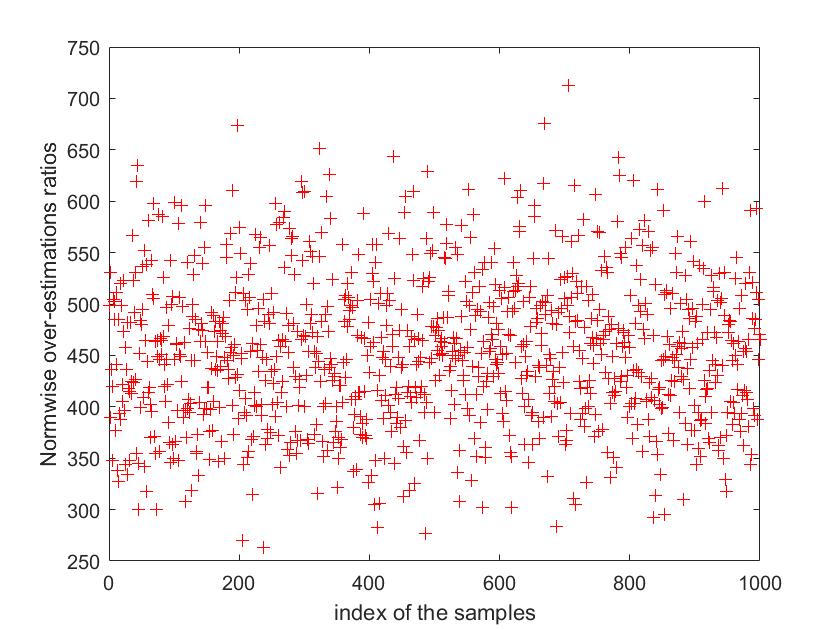
(a) Normwise over-estimation ratios

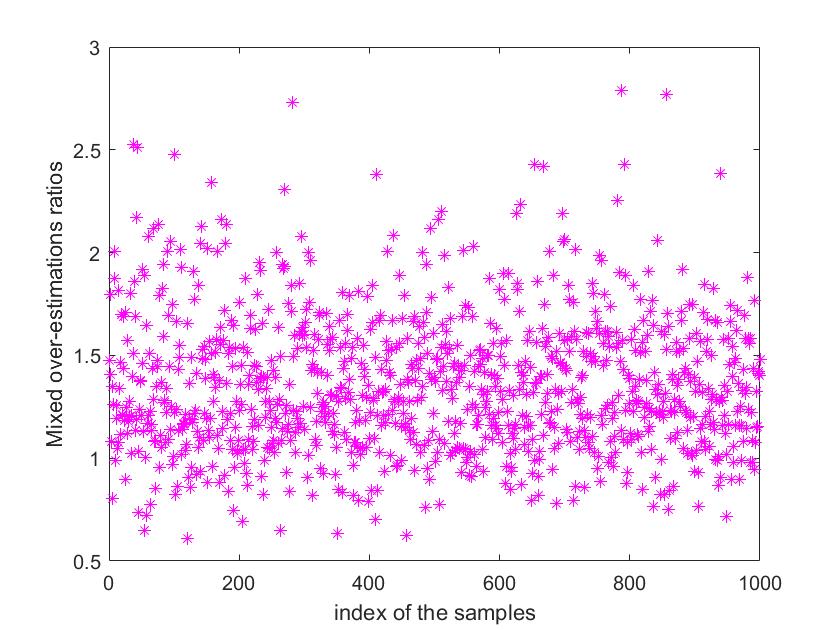
(b) Mixed over-estimation ratios

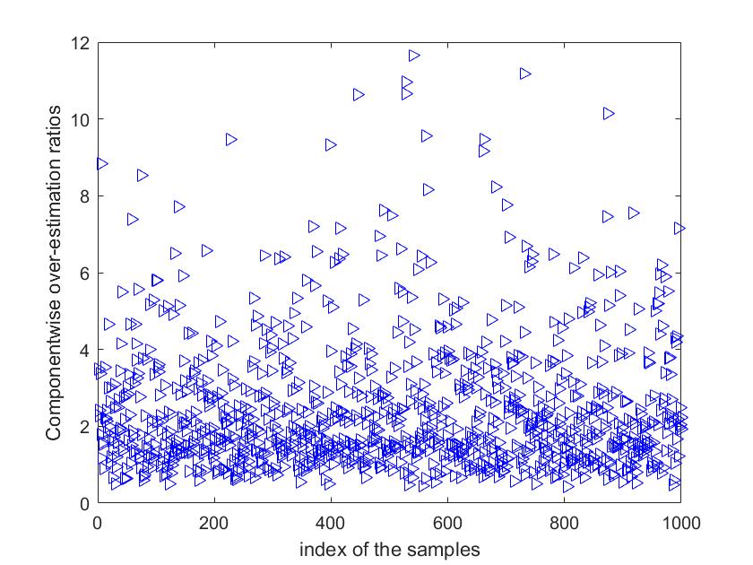
(c) Componentwise over-estimation ratios

Figure 1. SCE for the TLS problem under unstructured componentwise perturbations with 1000 samples for Example 5.3.

Figure 1 displays the numerical results for Example 5.3, where we generate 1000 random samples $[A~{}{\boldsymbol{b}}]$. From Figure 1, we see that $\kappa_{\rm SCE}^{\mathrm{TTLS},(\ell)}$ may seriously overestimate the true relative normwise error. All the normwise over-estimation ratios of 1000 samples is more than $10$, and the mean value of these estimations is $453.8841$. All elements of the mixed over-estimation ratios of 1000 samples are within $(0.1,~{}10)$ and the mean value of these estimations is $1.3563$. There are only 6 entries of the componentwise over-estimation ratios are greater than 10 and the mean value of these estimations is $2.4716$. The maximal values of the normwise, mixed and componentwise over-estimation vector are $712.5759,\,2.7908$ and $11.6508$, while their corresponding minimum are $263.3766,\,0.6078,0.4261$ accordingly. Therefore the mixed and componentwise condition estimations $m_{\rm SCE}^{\rm{TTLS},(\ell)}$ and $c_{\rm SCE}^{\rm{TTLS},(\ell)}$ are reliable.

Example 5.4.

Let the Toeplitz matrix $A$ and the vector ${\boldsymbol{b}}$ are defined in Example 5.2, where $m=500$. We generate 1000 structured componentwise perturbations $\Delta A_{1}=\epsilon\,(E_{1}\boxdot A)$ and 1000 unstructured componentwise perturbations $\Delta A_{2}=\epsilon\,(E_{2}\boxdot A)$, where $E_{1}$ is a random Toeplitz matrix and $E_{2}$ is a random matrix whose entries are uniformly distributed in the open internal $(-1,1)$. And $\Delta{\boldsymbol{b}}=\epsilon\,(f\boxdot{\boldsymbol{b}})$, where ${\boldsymbol{f}}$ is a random matrix with components uniformly distributing in the open interval $(-1,1)$.

For Example 5.4, we use $r_{\kappa}^{S}$, $r_{m}^{S}$ and $r_{c}^{S}$ to denote the structured normwise, mixed and componentwise over-estimation ratios corresponding to structured componentwise perturbations of $\Delta A_{1}$ and $\Delta{\boldsymbol{b}}$, and $r_{\kappa}$, $r_{m}$ and $r_{c}$ are unstructured normwise, mixed and componentwise over-estimation ratios corresponding to unstructured componentwise perturbations of $\Delta A_{2}$ and $\Delta{\boldsymbol{b}}$, where

$$r_{\kappa}^{\rm S}=\frac{\kappa_{\rm SCE}^{\mathrm{STTLS},(\ell)}\,\epsilon}{\|\tilde{\boldsymbol{x}}_{k}-{\boldsymbol{x}}_{k}\|_{2}/\|{\boldsymbol{x}}_{k}\|_{2}},\quad r_{m}^{\rm S}=\frac{m_{\rm SCE}^{\mathrm{STTLS},(\ell)}\,\epsilon}{\|\tilde{\boldsymbol{x}}_{k}-{\boldsymbol{x}}_{k}\|_{\infty}/\|{\boldsymbol{x}}_{k}\|_{\infty}},\quad r_{c}^{\rm S}=\frac{c_{\rm SCE}^{\mathrm{STTLS},(\ell)}\,\epsilon}{\|\frac{\tilde{\boldsymbol{x}}_{k}-{\boldsymbol{x}}_{k}}{{\boldsymbol{x}}_{k}}\|_{\infty}},$$

$$r_{\kappa}=\frac{\kappa_{\rm SCE}^{\mathrm{TTLS},(\ell)}\epsilon}{\|\tilde{\boldsymbol{x}}_{k}-{\boldsymbol{x}}_{k}\|_{2}/\|{\boldsymbol{x}}_{k}\|_{2}},\quad r_{m}=\frac{m_{\rm SCE}^{\mathrm{TTLS},(\ell)}\epsilon}{\|\tilde{\boldsymbol{x}}_{k}-{\boldsymbol{x}}_{k}\|_{\infty}/\|{\boldsymbol{x}}_{k}\|_{\infty}},\quad r_{c}=\frac{c_{\rm SCE}^{\mathrm{TTLS},(\ell)}\epsilon}{\|\frac{\tilde{\boldsymbol{x}}_{k}-{\boldsymbol{x}}_{k}}{{\boldsymbol{x}}_{k}}\|_{\infty}}.$$

Figure 2 displays the numerical results for Example 5.4 with $\ell=3$ and $\epsilon=10^{-8}$. Here, in Figure 2(A)–Figure 2(C), the symbol “+” in the blue color denote the numerical values of $r_{\kappa}^{\rm S}$, $r_{m}^{\rm S}$ and $r_{c}^{\rm S}$ corresponding to 1000 structured perturbations while the symbol “*” in the red color denote the numerical values of $r_{\kappa}$, $r_{m}$ and $r_{c}$ corresponding to 1000 unstructured perturbations.

From Figure 2, we observe that the mixed and componentwise condition estimations $m_{\rm SCE}^{\mathrm{STTLS},(\ell)}$, $c_{\rm SCE}^{\mathrm{STTLS},(\ell)}$, $m_{\rm SCE}^{\mathrm{TTLS},(\ell)}$ and $c_{\rm SCE}^{\mathrm{TTLS},(\ell)}$ are reliable, while the structured normwise condition estimation $\kappa_{\rm SCE}^{\mathrm{STTLS},(\ell)}$ may seriously over-estimate the true relative normwise error. Furthermore, we can also conclude that the over-estimation ratios associated with the structured mixed and component condition numbers are smaller than the unstructured counterparts in most cases, which are consistent with the conclusion in Proposition 2.1. The mean values of $r_{m}^{\rm S}$, $r_{m}$, $r_{c}^{\rm S}$, and $r_{c}$ of $1000$ samples are $1.7140$, $2.4642$, $1.7140$, and $2.4642$ respectively. Moreover, all these unstructured and structured mixed and componentwise condition over-estimation ratios are with $(0.1,10)$, which indicate mixed and componentwise condition estimations are reliable.

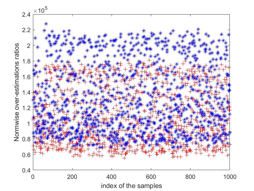
(a) Unstructured and structured normwise over-estimation ratios

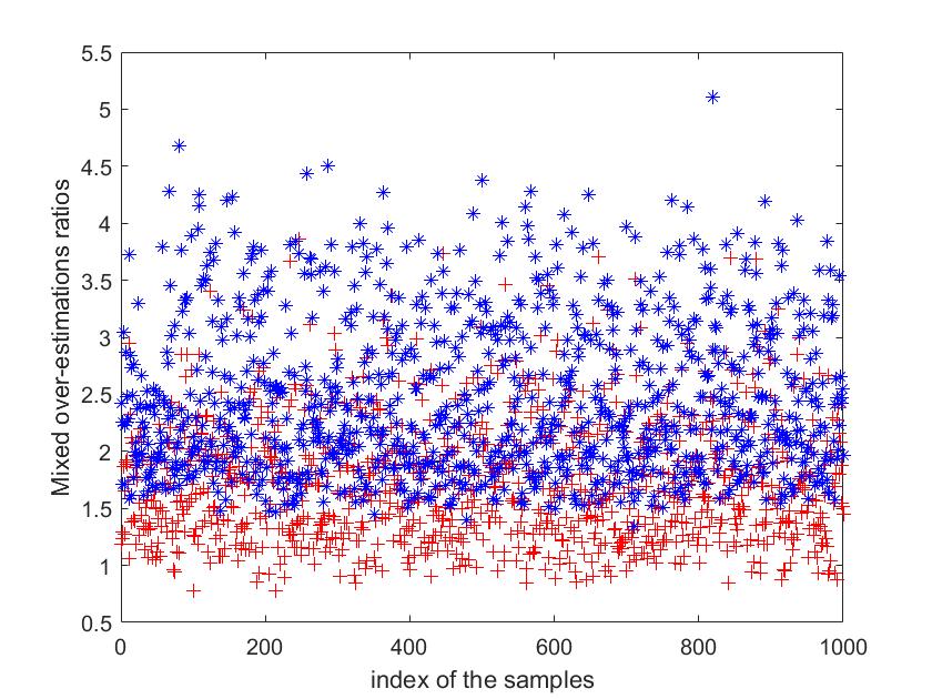
(b) Unstructured and structured mixed over-estimation ratios

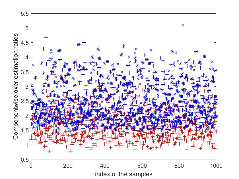
(c) Unstructured and structured componentwise over-estimation ratios

Figure 2. SCE for the TLS problem under unstructured and structured componentwise perturbations with 1000 unstructured and structured perturbations for Example 5.4.

Example 5.5.

This example comes from the model that restructures the image named Shepp-Logan “head phantom” (Shepp and Logan 1974) by the TTLS technique, which is widely used in inverse scattering studies. In fact, the TTLS method has been used to study the ultrasound inverse scattering imaging [24]. Here, we utilize the MATLAB file “paralleltomo.m” from the testprobs suite to create parallel-beam CT test problem and obtain the exact phantom. The input parameters of “paralleltomo.m” are set to be $N=40$, $\theta=0:5:175$, and $p=55$, hence we can obtain a $1834$-by-$1600$ matrix $A$ and $1834$-by-$1$ right-hand vector ${\boldsymbol{b}}$. The 500 perturbations $\Delta A$ and $\Delta{\boldsymbol{b}}$ of $A$ and ${\boldsymbol{b}}$ are generated as in (5.1).

Table 4 lists the condition estimations $\kappa_{\rm SCE}^{\mathrm{STTLS},(\ell)}$, $c_{\rm SCE}^{\mathrm{TTLS},(\ell)}$ and $m_{\rm SCE}^{\mathrm{TTLS},(\ell)}$ with truncation level $k=1536$ and the corresponding relative errors with respect to different magnitude $\epsilon$ of the perturbation for Example 5.5. From Table 4, we can see that the relative errors are bounded by the product of $\epsilon$ and corresponding condition estimations, which means that the proposed condition estimations can give reliable error bounds. The componentwise condition estimation $c_{\rm SCE}^{\mathrm{TTLS},(\ell)}$ is much larger than $\kappa_{\rm SCE}^{\mathrm{STTLS},(\ell)}$ and $m_{\rm SCE}^{\mathrm{TTLS},(\ell)}$ since the minimum absolute component of the TTLS solution ${\boldsymbol{x}}_{k}$ is too small, which is order of $10^{-6}$. Hence the component of the TTLS solution ${\boldsymbol{x}}_{k}$ in the sense of the tiny magnitude is very sensitive to small perturbations on the underlying component of ${\boldsymbol{x}}_{k}$.

Table 4. Comparison of the relative errors and SCE-based estimations by Algorithms 1 and 2 under 500 perturbations with different perturbation magnitudes for Example 5.5.

$\epsilon$	$10^{-1}$	$10^{-2}$	$10^{-3}$	$10^{-4}$	$10^{-5}$	$10^{-6}$	$10^{-7}$	$10^{-8}$
$\frac{\left\|\tilde{\boldsymbol{x}}_{k}-{\boldsymbol{x}}_{k}\right\|_{2}}{\|{\boldsymbol{x}}_{k}\|_{2}}$	$3.25\cdot 10^{-2}$	$3.25\cdot 10^{-3}$	$3.26\cdot 10^{-4}$	$3.26\cdot 10^{-5}$	$3.26\cdot 10^{-6}$	$3.26\cdot 10^{-7}$	$3.26\cdot 10^{-8}$	$3.26\cdot 10^{-9}$
$\kappa_{\rm SCE}^{\mathrm{TTLS},(\ell)}$	$3.33\cdot 10^{4}$	$3.33\cdot 10^{4}$	$3.33\cdot 10^{4}$	$3.33\cdot 10^{4}$	$3.33\cdot 10^{4}$	$3.333\cdot 10^{4}$	$3.33\cdot 10^{4}$	$3.33\cdot 10^{4}$
$\frac{\left\|\tilde{\boldsymbol{x}}_{k}-{\boldsymbol{x}}_{k}\right\|_{\infty}}{\|x_{k}\|_{\infty}}$	$2.62\cdot 10^{-2}$	$2.82\cdot 10^{-3}$	$2.89\cdot 10^{-4}$	$2.90\cdot 10^{-5}$	$2.90\cdot 10^{-6}$	$2.90\cdot 10^{-7}$	$2.90\cdot 10^{-8}$	$2.90\cdot 10^{-9}$
$m_{\rm SCE}^{\mathrm{TTLS},(\ell)}$	$3.74\cdot 10^{1}$	$3.74\cdot 10^{1}$	$3.74\cdot 10^{1}$	$3.74\cdot 10^{1}$	$3.74\cdot 10^{1}$	$3.74\cdot 10^{1}$	$3.74\cdot 10^{1}$	$3.74\cdot 10^{1}$
$\left\|\frac{\tilde{\boldsymbol{x}}_{k}-{\boldsymbol{x}}_{k}}{{\boldsymbol{x}}_{k}}\right\|_{\infty}$	$3.65\cdot 10^{2}$	$7.79\cdot 10^{1}$	$8.38\cdot 10^{0}$	$8.44\cdot 10^{-1}$	$8.44\cdot 10^{-2}$	$8.44\cdot 10^{-3}$	$8.44\cdot 10^{-4}$	$8.44\cdot 10^{-5}$
$c_{\rm SCE}^{\mathrm{TTLS},(\ell)}$	$1.85\cdot 10^{6}$	$1.85\cdot 10^{6}$	$1.85\cdot 10^{6}$	$1.85\cdot 10^{6}$	$1.85\cdot 10^{6}$	$1.85\cdot 10^{6}$	$1.85\cdot 10^{6}$	$1.85\cdot 10^{6}$

6. Concluding remarks

In this paper, we study the mixed and componentwise condition numbers of the TTLS problem under the genericity condition. We also consider the structured condition estimation for the STTLS problem and investigate the relationship between the unstructured condition numbers and the corresponding structured counterparts. When the TTLS problem degenerates the untrunctated TLS problem, we prove that condition numbers for the TTLS problem can recover the previous condition numbers for the TLS problem from their explicit expressions. Based on SCE, normwise, mixed and componentwise condition estimations algorithms are proposed for the TTLS problem, which can be integrated into the SVD-based direct solver for the TTLS problem. Numerical examples indicate that, in practice, it is better to adopt the componentwise perturbation analysis for the TTLS problem and the proposed algorithms are reliable, which provide posterior error estimations of high accuracy. The results in this paper can be extended to the truncated singular value solution of a linear ill-posed problem [2]. We will report our progresses on the above topic elsewhere in the future.

References

- [1] M. Baboulin and S. Gratton, A contribution to the conditioning of the total least-squares problem, SIAM J. Matrix Anal. Appl., 32(3) (2011), pp. 685–699.
- [2] E. H. Bergou, S. Gratton, and J. Tshimanga, The exact condition number of the truncated singular value solution of a linear ill-posed problem, SIAM J. Matrix Anal. Appl., 35(3) (2014), pp. 1073–1085.
- [3] A. Beck and A. Ben-Tal, A global solution for the structured total least squares problem with block circulant matrices, SIAM J. Matrix Anal. Appl., 27(1) (2005), pp 238–255.
- [4] H. Diao and Y. Sun, Mixed and componentwise condition numbers for a linear function of the solution of the total least squares problem, Linear Algebra Appl., 544 (2018), pp. 1–29.
- [5] H. Diao, Y. Wei, and P. Xie, Small sample statistical condition estimation for the total least squares problem, Numer. Algorithms, 75(2) (2017), pp. 435–455.
- [6] R. D. Fierro and J. R. Bunch, Collinearity and total least squares, SIAM J. Matrix Anal. Appl., 15(4) (1994), pp. 1167–1181.
- [7] R. D. Fierro and J. R. Bunch, Perturbation theory for orthogonal projection methods with applications to least squares and total least squares, Linear Algebra Appl., 234(2) (1996), pp. 71–96.
- [8] R. D. Fierro, G. H. Golub, P. C. Hansen, and D. P. O’Leary, Regularization by truncated total least squares, SIAM J. Sci. Comput., 18(4) (1997), pp. 1223–1241.
- [9] I. Gohberg and I. Koltracht, Mixed, componentwise, and structured condition numbers, SIAM J. Matrix Anal. Appl., 14(3) (1993), pp. 688–704.
- [10] G. Golub and W. Kahan, Calculating the singular values and pseudo-inverse of a matrix, J. SIAM Ser. B Numer. Anal., 2(2) (1965), pp. 205–224.
- [11] G. H. Golub and C. F. Van Loan, An analysis of the total least squares problem, SIAM J. Numer. Anal., 17(6) (1980), pp. 883–893.
- [12] G. H. Golub and C. F. Van Loan, Matrix Computations, 4th ed., Johns Hopkins University Press, Baltimore, MD, 2012.
- [13] A. Graham, Kronecker Products and Matrix Calculus: with Applications, Ellis Horwood, London, 1981.
- [14] S. Gratton, D. Titley-Peloquin, and J. T. Ilunga, Sensitivity and conditioning of the truncated total least squares solution, SIAM J. Matrix Anal. Appl., 34(3) (2013), pp. 1257–1276.
- [15] N. J. Higham, Accuracy and Stability of Numerical Algorithms, 2nd ed., SIAM, Philadelphia, PA, 2002.
- [16] Z. Jia and B. Li, On the condition number of the total least squares problem, Numer. Math., 125(1) (2013), pp. 61–87.
- [17] J. Kamm and J. G. Nagy, A total least squares method for Toeplitz systems of equations, BIT, 38(3) (1998), pp. 560–582.
- [18] C. S. Kenney and A. J. Laub, Small-sample statistical condition estimates for general matrix functions, SIAM J. Sci. Comput., 15(1) (1994), pp. 36–61.
- [19] C. S. Kenney, A. J. Laub, and M. S. Reese, Statistical condition estimation for linear least squares, SIAM J. Matrix Anal. Appl., 19(4) (1998), pp. 906–923.
- [20] C. S. Kenney, A. J. Laub, and M. S. Reese, Statistical condition estimation for linear systems, SIAM J. Sci. Comput., 19(2) (1998), pp. 566–583.
- [21] A. J. Laub and J. Xia, Applications of statistical condition estimation to the solution of linear systems, Numer. Linear Algebra Appl., 15 (2008), pp. 489–513.
- [22] P. Lemmerling and S. Van Huffel, Analysis of the structured total least squares problem for Hankel/Toeplitz matrices, Numer. Algorithms, 27(1) (2001), pp. 89–114.
- [23] B. Li and Z. Jia, Some results on condition numbers of the scaled total least squares problem, Linear Algebra Appl, 435(3) (2011), pp. 674–686.
- [24] C. Liu, Y. Wang and P. Heng, A comparison of truncated total least squares with Tikhonov regularization in imaging by ultrasound inverse scattering, Phy. in Med. Biol., 48(15) (2003), pp. 2437–2451.
- [25] I. Markovsky and S. Van Huffel, Overview of total least-squares methods, Signal Processing, 87(10) (2007), pp. 2283–2302.
- [26] R. D. Skeel, Scaling for numerical stability in Gaussian elimination, J. ACM, 26(3) (1979), pp. 494–526.
- [27] S. Van Huffel and J. Vandewalle, The Total Least Squares Problem: Computational Aspects and Analysis, SIAM, Philadelphia, PA, 1991.
- [28] M. Wei, The analysis for the total least squares problem with more than one solution, SIAM J. Matrix Anal. Appl., 13(3) (1992), pp. 746–763.
- [29] B. Zheng, L. Meng, and Y. Wei, Condition numbers of the multidimensional total least squares problem, SIAM J. Matrix Anal. Appl., 38 (2017), pp. 924–948.
- [30] B. Zheng and Z. Yang, Perturbation analysis for mixed least squares-total least squares problems, Numer Linear Algebra Appl., 26(4) (2019), e2239.
- [31] L. Zhou, L. Lin, Y. Wei, and S. Qiao, Perturbation analysis and condition numbers of scaled total least squares problems, Numer. Algorithms, 51(3) (2009), pp. 381–399.