Plane-wave approach to the exact van der Waals interaction between colloid particles

Abstract

The numerically exact evaluation of the van der Waals interaction, also known as Casimir interaction when including retardation effects, constitutes a challenging task. We present a new approach based on the plane-wave basis and demonstrate that it possesses advantages over the more commonly used multipole basis. The rotational symmetry of the plane-sphere and sphere-sphere geometries can be exploited by means of a discrete Fourier transform. The new technique is applied to a study of the interaction between a colloid particle made of polystyrene or mercury and another polystyrene sphere or a polystyrene wall in an aqueous solution. Special attention is paid to the influence of screening caused by a variable salt concentration in the medium. It is found that in particular for low salt concentrations the error implied by the proximity force approximation is larger than usually assumed. For a mercury droplet, a repulsive interaction is found for sufficiently large distances provided screening is negligible. We emphasize that the effective Hamaker parameter depends significantly on the scattering geometry on which it is based.

I Introduction

Aqueous colloidal suspensions play an important role in our daily lives, both in natural substances as well as in manifold industrial applications. For an understanding of their physical properties as well as for the design of such colloidal systems, a theoretical description of the relevant forces is required. In aqueous suspensions repulsive double layer electrostatic forces play a major role. Butt2010 ; Israelachvili2011 An important omnipresent interaction for all colloidal systems is the van der Waals force, Israelachvili2011 which is typically attractive but can be repulsiveDzyaloshinskii1961 ; Milling1996 ; Munday2009 ; Tabor2011 ; Thiyam2018 ; Esteso2019 for certain combinations of materials. These two forces are essential for understanding the stability of colloids.

Colloidal suspensions are composed of nano- to micrometer-size objects. For colloid particles less than $10\,\text{nm}$ apart, the fluctuating electromagnetic interaction can typically be treated as instantaneous while for larger separations retardation effects need to be taken into account. Butt2010 The retarded van der Waals force is often also referred to as Casimir force.Casimir1948 ; Lifshitz1956 ; Bordag2009 In this paper, we present exact theoretical results for the van der Waals force covering the entire distance range of experimental interest, while focusing on larger distances. In addition to retardation, non-trivial geometry effects become more important as the distance increases, making commonly employed approximations increasingly inaccurate.

As a minimal model for the study of aqueous colloidal systems, the interaction of two spherical particles in a solvent or the interaction between a spherical particle and a wall can be considered. Such situations have been realized in numerous experiments. Bevan1999 ; Hansen2005 ; Wodka2014 ; Ether2015 ; Montes2017 The plane-sphere and sphere-sphere setup are also typical for experiments exploring Casimir forces across vacuum or air. Klimchitskaya2009 ; Decca2011 ; Lamoreaux2011 ; Klimchitskaya2020

The finite curvature of the spherical particles is usually accounted for by means of the proximity force approximation (PFA), also known as Derjaguin approximation. Derjaguin1934 Within the PFA, the van der Waals interaction energy is calculated by averaging the energies of parallel planes over the local distances. Parsegian2005 The PFA can be understood as an asymptotic result where the sphere radius represents the largest length scale. Spreng2018 In order to determine its range of validity one needs to determine subleading correction terms or make use of numerical techniques.

Analytically, corrections to the PFA can be found through asymptotic expansions of the scattering-theoretical expression for the van der Waals energy Bordag2008 ; Teo2011 ; Teo2012 ; Teo2013 ; Henning2019 or by means of a derivative expansion.Fosco2011 ; BimonteEPL2012 ; BimonteAPL2012 ; Fosco2014 ; Fosco2015 Also, more recently a semi-analytical method utilizing the derivative expansion has been proposed.Bimonte2018a ; Bimonte2018b

Numerical methods for computing the van der Waals interaction complement analytical results beyond the PFA. They do not only serve as a quality check for approximations, but can yield exact results valid for any separation between the objects. Numerical approaches applicable to general geometries include the boundary-element method Reid2015 and simulations based on the finite-difference time-domain method. Oskooi2010

Specializing on spheres and possibly planes, larger aspect ratios between sphere radius and surface-to-surface distance are accessible by making use of the scattering formalism. Lambrecht2006 ; Emig2007 For such geometries, bispherical coordinates might appear as an efficient tool to derive the relevant scattering operators. However, only the Laplace equation and not the Helmholtz equation is separable in these coordinates.Boyer76 In practice, their use is thus limited to the zero-frequency contribution of the van der Waals interaction. Bimonte2017 ; Bimonte2018b The contribution of arbitrary frequencies is computed by expressing the scattering operators referring to the individual surfaces in appropriately chosen local coordinate systems. For numerical purposes, the scattering operators as well as the translation operators connecting the two coordinate systems have to be expressed in a suitable basis. Spherical multipoles have been used in numerous studies of scattering geometries composed of a plane and a sphere, MaiaNeto2008 ; Emig2008 ; Canaguier-Durand10 ; Canaguier-Durand-thesis ; Canaguier-Durand12 two spheres Emig2007 ; Umrath2015 or a grating and a sphere. Messina2015 While for large distances, it is sufficient to take into account only a few multipoles, the situation changes dramatically when experimentally relevant aspect ratios are considered. This range became accessible only recently by symmetrization of the scattering operator and employing hierarchical low-rank approximation techniques. Hartmann2017 ; Hartmann2018 ; HartmannThesis

In this paper, we will develop an alternative numerical approach making use of the plane-wave basis, which is better adapted to capture the effect of near specular reflection in the vicinity of the WKB scattering regime, Spreng2018 while still allowing for arbitrary temperatures and materials. The convergence properties of our approach will turn out to be far superior to those found for the spherical multipole basis. Often, scattering operators are already known in the plane-wave basis as scattering amplitudes vdHulst derived for different geometries by making use of the appropriate coordinate systems.Boyer76 In addition, this basis makes translations between the coordinate systems employed for each particle particularly simple. In comparison with the spherical multipole basis, the non-discreteness of the plane-wave basis might appear as an important drawback. However, as we will discuss in this paper, the problem can be circumvented in a natural way by means of a Nyström discretization of the plane-wave momenta. As a consequence, our method based on the the plane-wave basis turns out to be easier to implement than the more standard multipolar approach.

As an illustration of this new numerical plane-wave approach, we will consider two polystyrene microspheres in an aqueous solution and compare the PFA with the numerically computed van der Waals interaction. In contrast to the work by Thennadil and Garcia-Rubio, Thennadil2001 our comparison is exact and goes beyond the perturbative approach developed by Langbein. Langbein1970 ; Langbein1974 Likewise, we study the van der Waals interaction between a polystyrene microsphere and a polystyrene wall. The exact results for the two polystyrene surfaces in the plane-sphere and sphere-sphere geometry then allow us to study the geometry dependence of the Hamaker parameter. We finally conduct an analogous analysis for the system of a mercury microsphere and a polystyrene surface. The van der Waals interaction of such systems can be repulsive or attractive depending on how the distance between the surfaces compares with the Debye screening length.Ether2015

This paper is structured as follows. In Sec. II, the numerical method is introduced first for arbitrary scatterers and then specialized to geometries with a cylindrical symmetry. In Sec. III, we apply the method to the plane-sphere and sphere-sphere geometries. The convergence properties of our numerical approach are studied for both examples. Furthermore, for the plane-sphere geometry we compare the computational time needed with the plane-wave approach and a reference implementation based on spherical multipoles. HartmannJOSS In Sec. IV, we apply the plane-wave method to the analysis of the van der Waals interaction in colloidal systems containing polystyrene or mercury spheres. Sec. V contains concluding remarks and the appendices provide technical details supporting the main text of the paper.

II van der Waals interaction within the plane-wave basis

II.1 Geometry of two arbitrary objects

We will consider two arbitrary objects 1 and 2 immersed in a homogeneous medium at temperature $T$ and assume that the objects can be spatially separated by a plane. Within the scattering-theoretical approach, the van der Waals free energy of this setup is given by Lambrecht2006

$$\mathcal{F}=\frac{k_{B}T}{2}\sum_{n=-\infty}^{\infty}\log\det\left[1-\mathcal{M}(|\xi_{n}|)\right]$$ (1)

with the Matsubara frequencies $\xi_{n}=2\pi nk_{B}T/\hbar$ and the round-trip operator

$$\mathcal{M}=\mathcal{T}_{12}\mathcal{R}_{2}\mathcal{T}_{21}\mathcal{R}_{1}\,.$$ (2)

$\mathcal{R}_{j}$ denotes the reflection operator of object $j$ with respect to the reference point $\mathcal{O}_{j}$ while $\mathcal{T}_{21}$ carries out the translation from the reference point of object $1$ to the one of object $2$, and vice versa for $\mathcal{T}_{12}$. The two reference points $\mathcal{O}_{1}$ and $\mathcal{O}_{2}$ are separated by a distance $\mathcal{L}$ and define the $z$-axis of our coordinate system. Figure 1 schematically depicts the full round trip described by $\mathcal{M}$.

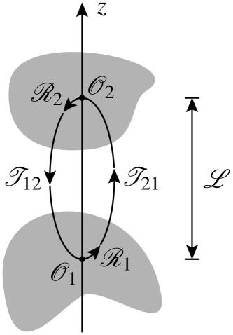
Figure 1: Schematic representation of the scattering geometry containing two objects 1 and 2. Their respective reference points $\mathcal{O}_{1}$ and $\mathcal{O}_{2}$ define the $z$-axis and are separated by a distance $\mathcal{L}$.

By taking the derivative of (1) with respect to the distance $\mathcal{L}$, one obtains the van der Waals force

$$F=-\partial_{\mathcal{L}}\mathcal{F}=\frac{k_{B}T}{2}\sum_{n=-\infty}^{\infty}\mathrm{tr}\left[\frac{\partial_{\mathcal{L}}\mathcal{M}}{1-\mathcal{M}}\right]$$ (3)

where we dropped the dependence of the round-trip operator on the Matsubara frequencies $\xi_{n}$. A corresponding formula for the force gradient can be found for instance in Ref. Bimonte2018b, .

The frequency of a plane wave is conserved during a round trip between the two objects. Thus, it is convenient to employ the so-called angular spectral representation.NietoVesperinas Within this representation, $\{\ket{\xi,\mathbf{k},\phi,p}\}$ denotes the plane-wave basis at imaginary frequency $\xi$ where $\mathbf{k}$ is the transverse wave vector perpendicular to the $z$-axis, $\phi=\pm 1$ the upward or downward propagation direction and $p=\mathrm{TE},\mathrm{TM}$ the polarization. Because $\xi$ remains unchanged during the round trip and $\phi$ only changes sign after reflection off an object, we shorten the notation of the basis elements to $\ket{\mathbf{k},p}$.

The translation operators $\mathcal{T}_{12}$ and $\mathcal{T}_{21}$ are diagonal in the plane-wave basis with matrix elements $e^{-\kappa\mathcal{L}}$. The axial wave vector after Wick rotation is given by

$$\kappa=\left(\epsilon_{m}\frac{\xi^{2}}{c^{2}}+\mathbf{k}^{2}\right)^{1/2}\,,$$ (4)

where $\epsilon_{m}$ denotes the relative permittivity of the medium between the two objects. In contrast, the reflection operators $\mathcal{R}_{1}$ and $\mathcal{R}_{2}$ and thus the round-trip operator $\mathcal{M}$ will not be diagonal in general. The latter operators are integral operators which can be expressed in terms of their respective kernel functions. For example the round-trip operator can be written as

$$\mathcal{M}\ket{\mathbf{k},p}=\sum_{p^{\prime}}\int\frac{d\mathbf{k}^{\prime}}{(2\pi)^{2}}\,K_{\mathcal{M}}(\mathbf{k^{\prime}},p^{\prime};\mathbf{k},p)\ket{\mathbf{k}^{\prime},p^{\prime}}$$ (5)

with its kernel function

$$K_{\mathcal{M}}(\mathbf{k^{\prime}},p^{\prime};\mathbf{k},p)=\\ e^{-\kappa^{\prime}\mathcal{L}}\sum_{p^{\prime\prime}}\int\frac{d\mathbf{k}^{\prime\prime}}{(2\pi)^{2}}\,K_{\mathcal{R}_{2}}(\mathbf{k^{\prime}},p^{\prime};\mathbf{k^{\prime\prime}},p^{\prime\prime})e^{-\kappa^{\prime\prime}\mathcal{L}}\\ \times K_{\mathcal{R}_{1}}(\mathbf{k^{\prime\prime}},p^{\prime\prime};\mathbf{k},p)\,,$$ (6)

where $K_{\mathcal{R}_{j}}$ is the kernel of the reflection operator $\mathcal{R}_{j}$ for $j=1,2$ and $\kappa^{\prime}$ as well as $\kappa^{\prime\prime}$ are defined according to (4). Note that the kernel functions depend also on the frequency $\xi$ which is suppressed in the arguments to not overload the notation.

For numerical purposes, a Nyström discretization needs to be applied to the integral appearing in (5). The action of the round-trip operator is then expressed in terms of a finite matrix

$$\mathcal{M}\ket{\mathbf{k}_{\alpha},p}=\sum_{p^{\prime},\alpha^{\prime}}\frac{w_{\alpha^{\prime}}}{(2\pi)^{2}}K_{\mathcal{M}}(\mathbf{k}_{\alpha^{\prime}},p^{\prime};\mathbf{k}_{\alpha},p)\ket{\mathbf{k}_{\alpha^{\prime}},p^{\prime}}$$ (7)

with the nodes $\mathbf{k}_{\alpha}$ and weights $w_{\alpha}$ of a quadrature rule for the two-dimensional integral. The indices $\alpha$ and $\alpha^{\prime}$ represent tuples $(i,j)$ where $i$ and $j$ are indices from the quadrature rules of the corresponding one-dimensional integrals.

Within this approximation the matrix elements of the round-trip operator become the corresponding kernel function multiplied by the quadrature weights Bornemann2010

$$\braket{\mathbf{k}_{\alpha^{\prime}},p^{\prime}}{\mathcal{M}}{\mathbf{k}_{\alpha},p}=\frac{w_{\alpha^{\prime}}}{(2\pi)^{2}}K_{\mathcal{M}}(\mathbf{k}_{\alpha^{\prime}},p^{\prime};\mathbf{k}_{\alpha},p)\,.$$ (8)

After discretization the matrix elements thus form a three-fold block matrix with respect to the two indices constituting the tuple $\alpha=(i,j)$ and the polarization $p$.

In general, the reflection operators pertaining to the two objects are non-diagonal in the plane-wave basis as is the case for example in the geometry of two spheres. The integral over $\mathbf{k}^{\prime\prime}$ appearing inside the kernel of the round-trip operator (6) can usually not be performed analytically. Thus, for numerical applications this integral needs to be discretized as well where the quadrature rule may differ from the one chosen in (7). The round-trip matrix can then be expressed in terms of a product of two block matrices representing the reflection operators.

II.2 Geometry with cylindrical symmetry

Casimir and van der Waals experiments are often carried out in set-ups with a certain symmetry. The cylindrical symmetry is particularly common as it appears in the plane-sphere and sphere-sphere geometries. At first sight, the spherical-wave basis appears to be better adapted for those geometries since the angular momentum index $m$ is conserved through the round trip, yielding a block-diagonal round-trip matrix. However, this symmetry can also be exploited in the plane-wave basis as will be explained in the following.

For a cylindrically symmetric geometry it is natural to express the transverse wave vector $\mathbf{k}$ in polar coordinates with radial component $k$ and angular component $\varphi$, where the latter is relevant for the following considerations. A suitable quadrature rule for the integration over $\varphi$ is the trapezoidal rule which at order $M$ has nodes at $\varphi_{j}=(2\pi/M)j$ with constant weights $w_{j}=2\pi/M$ where $j=1,\dots,M$.

Due to the cylindrical symmetry, the kernel functions depend only on the difference of the angular components $\Delta\varphi=\varphi^{\prime}-\varphi$. Because the weights of the trapezoidal rule are constant and its nodes proportional to the indices, the discretized block matrix then depends through the difference of the angles only on the difference of the indices, i.e. $\Delta\varphi_{i,j}=\Delta\varphi_{i-j}$. Such a block matrix is called circulant and can be block-diagonalized by a discrete Fourier transform. The blocks on the diagonal then correspond to the contributions for each angular momentum index starting from $m=0,\pm 1,\dots$ up to $\pm(M-1)/2$ when $M$ is odd or $M/2$ when $M$ is even. Note that opposite signs in the angular momentum index contribute equally. This is due to the fact that angular momentum indices of opposite signs are connected through the Fourier transform by the transformation $\Delta\varphi\rightarrow-\Delta\varphi$. Such a transformation, however, leaves the van der Waals interaction unchanged, since it corresponds to a flip in the sign of the $z$-coordinates.

The reflection operators of the two objects may in general be non-diagonal as it is the case in the geometry of two spheres. In Sec. II it was argued that the discretized round-trip matrix can then be written in terms of a product of two block matrices. In order to exploit the cylindrical symmetry, the quadrature rule of the angular component of the $\mathbf{k}^{\prime\prime}$-integral in (6) needs to be a trapezoidal rule of the same order $M$ as above. Only then both block matrices become circulant such that after the discrete Fourier transform their block matrix product can be simplified to a product of block-diagonal matrices.

It is possible to perform the discrete Fourier transform analytically, which opens the possibility for a hybrid numerical method in which the matrix elements are constructed by discretizing the radial transverse momentum $k$ for each angular momentum index $m$. At first sight, one might favor such a hybrid approach over the pure plane-wave approach discussed above, since one can save on the computation time of the discrete Fourier transform. In practice, however, the time needed for the discrete Fourier transform in the plane-wave approach is dominated by the computation of the matrix elements. Numerical tests on the plane-sphere geometry indicate that the hybrid approach is slower than the plane-wave approach.

III Application to geometries involving spheres

The plane-wave method described in the previous section will now be applied to colloidal systems involving spheres. First, we discuss the scattering of plane waves at a sphere. Then we study the plane-wave method for the plane-sphere and the sphere-sphere geometries. Both scattering geometries are cylindrically symmetric so that the simplification discussed in Sec. II.2 applies.

III.1 Plane-wave scattering at a sphere

For a sphere of radius $R$, the kernel of the reflection operator is given by

$$K_{\mathcal{R}_{\mathrm{S}}}(k,\varphi,\mathrm{TM};k^{\prime},\varphi^{\prime},\mathrm{TM}) =\frac{2\pi\lambdabar_{m}k}{\kappa}\left[AS_{2}+BS_{1}\right]$$ (9)

$$K_{\mathcal{R}_{\mathrm{S}}}(k,\varphi,\mathrm{TE};k^{\prime},\varphi^{\prime},\mathrm{TE}) =\frac{2\pi\lambdabar_{m}k}{\kappa}\left[AS_{1}+BS_{2}\right]$$

$$K_{\mathcal{R}_{\mathrm{S}}}(k,\varphi,\mathrm{TM};k^{\prime},\varphi^{\prime},\mathrm{TE}) =-\frac{2\pi\lambdabar_{m}k}{\kappa}\left[CS_{1}+DS_{2}\right]$$

$$K_{\mathcal{R}_{\mathrm{S}}}(k,\varphi,\mathrm{TE};k^{\prime},\varphi^{\prime},\mathrm{TM}) =\frac{2\pi\lambdabar_{m}k}{\kappa}\left[CS_{2}+DS_{1}\right]$$

with the imaginary angular wavelength in the medium

$$\lambdabar_{m}=\frac{c}{\sqrt{\epsilon_{m}}\xi}\,.$$ (10)

Explicit expressions for the Mie scattering amplitudes $S_{1}$ and $S_{2}$ are given below. As these scattering amplitudes are taken with respect to a polarization basis referring to the scattering plane, the rotation into the polarization basis of TE and TM modes defined with respect to the $z$-axis gives rise to the coefficients $A$, $B$, $C$, and $D$ specified in Appendix A. For convenience, the factor $k$ arising from the integration measure in polar coordinates has been absorbed into the kernel functions.

The Mie scattering amplitudes for plane waves with polarization perpendicular and parallel to the scattering plane are defined through an expansion in terms of partial waves with angular momentum $\ell$ as (Kvien1998, ; BH, )

$$S_{1} =\sum_{\ell=1}^{\infty}\frac{2\ell+1}{\ell(\ell+1)}\left[a_{\ell}\pi_{\ell}\big{(}\cos(\Theta)\big{)}+b_{\ell}\tau_{\ell}\big{(}\cos(\Theta)\big{)}\right]$$ (11)

$$S_{2} =\sum_{\ell=1}^{\infty}\frac{2\ell+1}{\ell(\ell+1)}\left[a_{\ell}\tau_{\ell}\big{(}\cos(\Theta)\big{)}+b_{\ell}\pi_{\ell}\big{(}\cos(\Theta)\big{)}\right]\,,$$

respectively. The Mie coefficients $a_{\ell}$ and $b_{\ell}$ for electric and magnetic polarizations, respectively, depend on the electromagnetic response of the homogeneous sphere and are evaluated at the imaginary size parameter $R/\lambdabar_{m}$.

The angle $\Theta$ between the directions of the outgoing and incoming wave is given through

$$\cos(\Theta)=-\lambdabar_{m}^{2}\left[kk^{\prime}\cos(\varphi-\varphi^{\prime})+\kappa\kappa^{\prime}\right]\,.$$ (12)

The angular functions BH

$$\pi_{\ell}(z) ={P_{\ell}}^{\prime}(z)$$ (13)

$$\tau_{\ell}(z) =-(1-z^{2}){P_{\ell}}^{\prime\prime}(z)+z{P_{\ell}}^{\prime}(z)\,,$$

are expressed in terms of Legendre polynomials $P_{\ell}(z)$ and the prime indicates a derivative with respect to the argument $z=\cos(\Theta)$.

III.2 Plane-sphere geometry

For a sphere with radius $R$ above a plane at a surface-to-surface distance $L$, the kernel of the round-trip operator is given by

$$K_{\mathcal{M}}(\mathbf{k},p;\mathbf{k^{\prime}},p^{\prime})=r_{p}e^{-(\kappa+\kappa^{\prime})(L+R)}K_{\mathcal{R}_{\mathrm{S}}}(\mathbf{k},p;\mathbf{k^{\prime}},p^{\prime})$$ (14)

with the Fresnel coefficients $r_{p}$ given in Appendix B and the kernel of the reflection operator at the sphere $K_{\mathcal{R}_{\mathrm{S}}}$ defined in Eq. (9). The exponential function corresponds to the translation of the plane waves from the plane to the sphere center and back.

In the multipole method, a symmetrization of the round-trip operator is important for a fast and stable numerical evaluation of the van der Waals interaction because otherwise the matrices appearing in the calculation are ill-conditioned.Hartmann2018 This symmetrization is not as crucial in the plane-wave method where it merely gives a factor of two in run-time speed-up because only half of the matrix elements need to be computed.

It is however important to write the translation over the sphere radius in (14) symmetrically with respect to the two momenta $\kappa$ and $\kappa^{\prime}$. Only then the matrix elements in the plane-wave method are well-conditioned and take their maximum around $\mathbf{k}=\mathbf{k}^{\prime}$. This can be understood by examining the asymptotic behavior of the round-trip operator when $R\gg L$. By employing the asymptotics of the scattering amplitudes for large radii,Nussenzveig69 ; Nussenzveig92 the leading $R$-dependent contribution of the kernel of the round-trip operator can be identified as the exponential factor Spreng2018 ; Henning2019

$$\exp\left\{-\frac{R}{\lambdabar_{m}}\left[\lambdabar_{m}(\kappa+\kappa^{\prime})-2\sin\left(\frac{\Theta}{2}\right)\right]\right\}\,.$$ (15)

with the angle $\Theta$ defined through (12). Its main contribution comes from $k=k^{\prime}$ and $\varphi=\varphi^{\prime}$ where the exponent vanishes. When the translation operator is not expressed symmetrically with respect to the momenta, the kernel would grow exponentially with $\kappa$ and decrease exponentially with $\kappa^{\prime}$ or vice versa, resulting in an ill-conditioned matrix.

III.2.1 Quadrature rule for radial wave vector component

Before the van der Waals interaction can be determined numerically, the quadrature rule for the integration over the radial component of the transverse wave vectors in (7) needs to be specified. In principle, any quadrature rule for the semi-infinite interval $[0,\infty)$ can be used. The Fourier-Chebyshev scheme described in Ref. Boyd1987, turned out to be particularly well suited. Defining

$$t_{n}=\frac{\pi n}{N+1}\,,$$ (16)

the quadrature rule is specified by its nodes

$$k_{n}=b\cot^{2}(t_{n}/2)$$ (17)

and weights

$$w_{n}=\frac{8b\sin(t_{n})}{[1-\cos(t_{n})]^{2}}\frac{1}{N+1}\sum_{\begin{subarray}{c}j=1\\ \text{$j$ odd}\end{subarray}}^{N}\frac{\sin(jt_{n})}{j}$$ (18)

for $n=1,\dots,N$. An optimal choice for the free parameter $b$ can boost the convergence of the computation.

For dimensional reasons, the transverse wave vector and thus $b$ should scale like the inverse surface-to-surface distance $1/L$. In fact, the choice $b=1/L$ already yields a fast convergence rate and will be used in the following discussion.

III.2.2 Estimation of the convergence rate

In order to understand how well the plane-wave method performs when $R\gg L$, one needs to know how the quadrature orders $N$ and $M$ for the integration over the angular and radial wave vector component, respectively, scale with the aspect ratio $R/L$ for a maximally allowed relative error. We refer to this scaling as the convergence rate of the quadrature schemes.

In the multipole method, the number of multipoles needs to be truncated in order to make the calculation of the van der Waals interaction amenable to linear algebra routines. Convergence will then be reached when the highest multipole index $\ell_{\mathrm{max}}$ and the highest angular momentum index $m_{\mathrm{max}}$ included in the computation take values which scale as $\ell_{\mathrm{max}}\sim R/L$ and $m_{\mathrm{max}}\sim\sqrt{R/L}$, respectively.Teo2011 ; Teo2012 ; Teo2013 Since the angular quadrature order $M$ in the plane-wave approach is related to $m_{\mathrm{max}}$ through a Fourier transform, one can expect that it exhibits the same convergence rate as $m_{\mathrm{max}}$. The scaling behavior of the radial quadrature order $N$, however, is a priori not known and will be determined in the following.

Within the plane-wave approach, convergence can only be reached once the nodes associated to the quadrature rules are able to resolve the structure of the kernel functions. The important contributions of the round-trip kernel come from a region around its maximum at $\kappa=\kappa^{\prime}\approx 1/L$. This region corresponds to indices of the Fourier-Chebyshev quadrature rule around $n=n^{\prime}\approx N/2$, where for large $N$ the spacing between neighboring quadrature nodes is given by

$$\delta k\approx\frac{2\pi}{LN}\,.$$ (19)

Furthermore, when $R\gg L$, the kernel can be approximated by a Gaussian with width $\sqrt{\kappa/R}\sim 1/\sqrt{LR}$. This can be seen by expanding the exponent in (15) around $k=k^{\prime}$. Requiring $\delta k$ to be of the order of that Gaussian width, we find that the quadrature order $N$ scales like $\sqrt{R/L}$. Along the same lines, it can be verified that the angular quadrature order $M$ obeys the same scaling law.

The quadrature orders for angular and radial integration can thus be expressed as

$$N=\left\lceil\eta_{N}\left(\frac{R}{L}\right)^{1/2}\right\rceil\,,\quad M=\left\lceil\eta_{M}\left(\frac{R}{L}\right)^{1/2}\right\rceil\,$$ (20)

respectively, where the ceiling function ensures that the orders are integers. The two coefficients $\eta_{N}$ and $\eta_{M}$ control the numerical accuracy with larger values corresponding to higher accuracy.

Figure 2: The relative error as a function of $\eta_{N}$ (circles and crosses) and $\eta_{M}$ (squares and pluses) for the aspect ratios $R/L=50$ and $500$.

These expectations for the convergence rate can be verified numerically. We specifically consider perfect reflectors in vacuum, a sphere radius of $1\,\mu{\rm m}$, i.e. a typical value for colloids, and room temperature, $T=293\,{\rm K}$. Figure 2 shows the relative error of the van der Waals free energy as a function of $\eta_{N}$ and $\eta_{M}$ for the aspect ratios $R/L=50$ and $500$. The errors have been computed relative to energies with much larger values of the coefficients, namely $\eta_{N}=\eta_{M}=14$ for all points in the figure. For the points where the relative errors are shown as a function of $\eta_{N}$, the coefficient of the angular quadrature order was kept fixed at $\eta_{M}=14$, and vice versa. One can indeed see that the coefficients depend only weakly on the aspect ratio $R/L$. This also holds for other system parameters and materials of the objects. The figure can be further used as a guide to choose $\eta_{N}$ and $\eta_{M}$ in order to obtain a given numerical accuracy. The formulas (20) only work when $R/L$ is larger than 50. For smaller aspect ratios, one can simply set $R/L$ to $50$ in Eq. (20), which gives a sufficiently high accuracy depending on the coefficients $\eta_{N}$ and $\eta_{M}$.

In comparison to the multipole method we conclude that the matrix sizes appearing in the plane-wave approach are smaller by a factor of $\sqrt{R/L}$. This reduction in the matrix size becomes particularly relevant when typical aspect ratios appearing in experiments are considered.

III.2.3 Runtime analysis: plane-wave versus multipole method

We now further quantify the advantages of the plane-wave method over the multipole method by analyzing their respective runtimes. The plane-wave method was implemented in Python using the scientific libraries NumPy,numpy SciPyscipy as well as Numbanumba for just-in-time compilation. For the multipole method the implementation of Ref. HartmannJOSS, in C was used. Because the latter only supports the computation of the van der Waals free energy, we restrict the analysis to this quantity.

We consider the same plane-sphere setup as in Sec. III.2.2 with perfect reflectors in vacuum, a sphere radius of $R=1\,\mu{\rm m}$ and temperature $T=293\,{\rm K}$. The van der Waals free energy at finite temperatures can be evaluated in different ways. We consider the Matsubara spectrum decomposition (MSD) represented by Eq. (1), and the Padé spectrum decomposition (PSD) Hu2010 outlined in Appendix C. When using PSD, only $\sqrt{\lambda_{T}/L}$ terms in the frequency summation need to be considered, where $\lambda_{T}=\hbar c/k_{B}T$ is the thermal wavelength. Thus, PSD is expected to be significantly faster than MSD for all experimentally relevant distances since the latter requires a summation over $\lambda_{T}/L$ terms to ensure convergence.

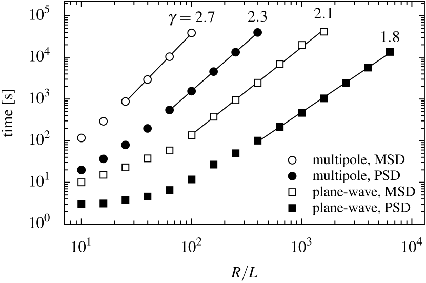
Figure 3: Runtime comparison between the plane-wave method (squares) and the multipole method (circles) using MSD (open symbols) and PSD (filled symbols). The solid lines indicate a power-law fit $\sim(R/L)^{\gamma}$ on the basis of the data points shown on top of the lines. The value of the exponent $\gamma$ is indicated at the end of the lines. The timing experiments were carried out on a computer with an Intel Core i7-2600 processor. The four cores running at $3.4\,{\rm GHz}$ were fully exploited by running eight threads or processes in parallel.

To ensure comparability, the van der Waals free energy is computed with both methods to the same numerical precision of about six correct digits. Figure 3 shows the runtime of the van der Waals free energy for the multipole method (circles) and the plane-wave method (squares) for aspect ratios $R/L\geq 10$ using MSD (open symbols) and PSD (filled symbols). For all timing experiments a machine with an Intel Core i7-2600 processor was used. The four cores running at $3.4\,{\rm GHz}$ were fully exploited by either running eight threads or processes in parallel depending on the implementation. We find that the plane-wave method is significantly faster than the multipole method. As expected, the PSD performs better than the MSD. For instance, at the aspect ratio $R/L=100$, the multipole methods takes about 11 hours to compute the free energy using MSD and only 25 minutes with PSD. The plane-wave method, however, needs only about two minutes to compute the same quantity when using MSD and 12 seconds with PSD. For other system parameters and materials we come to similar conclusions for the runtime.

The black lines in Fig. 3 are fits to the points they overspan. The timings of the multipole method are consistent with the timing experiment in Ref. Hartmann2018, where it was found that for a given frequency and angular momentum index the timing scales as $\sim(R/L)^{1.31}$. The sum over the angular momentum indices scales with $\sim(R/L)^{0.5}$. The above mentioned scaling behavior for the frequency sum in the MSD and PSD is thus consistent with the observed over-all scaling of $(R/L)^{2.7}$ and $(R/L)^{2.3}$, respectively.

The method based on plane waves scales as $(R/L)^{2.1}$ for MSD and $(R/L)^{1.8}$ using PSD, allowing the computation of higher aspect ratios with ordinary hardware. The difference between the scaling behavior of the MSD and PSD for the plane-wave method of about $(R/L)^{0.3}$ is notably smaller than the expected difference of $(R/L)^{0.5}$. As discussed in appendix C, while the PSD requires the evaluation of fewer frequency contributions to the Casimir energy, some of the frequencies to be considered are higher than those required for the MSD. Numerical tests show that the time needed to evaluate matrix elements increases with increasing frequency, thus offering an explanation for the reduced improvement of the PSD over the MSD.

Note that for the calculations of the determinants, we did not use the sophisticated algorithm using hierarchical matrices which was crucial to boost the performance for Casimir computations in the multipole basis.Hartmann2017 ; Hartmann2018 Since we are dealing with much smaller matrices and our computation time is dominated by the calculation of the matrix elements itself, such method is not expected to bring a significant improvement. Instead we speed up the calculation of the matrix elements by first estimating their values in terms of their asymptotic behavior given in Eq. (15). Since the matrices are well-conditioned and their dominant contributions come from matrix elements around the diagonal, we can set matrix-elements to zero if their asymptotic behavior predicts a value smaller than the machine precision. Otherwise, the computed matrix elements are numerically exact. Numerical tests reveal that this scheme yields a speed-up scaling as $(R/L)^{0.5}$.

III.3 Sphere-sphere geometry

Another example of a van der Waals setup with cylindrical symmetry consists of two spheres with radii $R_{1}$ and $R_{2}$. As in the plane-sphere geometry, we denote the surface-to-surface distance as $L$. The kernel of the round-trip operator is of the form (6) with the kernel functions of the reflection operators of the respective spheres given in (9). Note that the sign of the coefficients $C$ and $D$ differs for the two spheres.

We recall that, because the reflection operator at both objects is now non-diagonal, a discretization of two integrals over the transverse momenta is required. Firstly, the discretization of the integral over $\mathbf{k}^{\prime}$ in Eq. (5) results in a finite matrix representation of the round-trip operator. Secondly, the discretization of the integral over $\mathbf{k}^{\prime\prime}$ in Eq. (6) allows to express the round-trip matrix in terms of a product of two block-matrices. For the radial components we employ the Fourier-Chebyshev quadrature scheme presented in Sec. III.2.1. The quadrature orders, however, do not need to coincide and thus we use the quadratures of order $N^{\prime}$ and $N^{\prime\prime}$ for the integrations over $k^{\prime}$ and $k^{\prime\prime}$, respectively. Likewise we employ trapezoidal rules of order $M^{\prime}$ and $M^{\prime\prime}$ for the discretization of the angular components. In order to exploit the cylindrical symmetry of the problem by means of the discrete Fourier transform, the quadrature orders $M^{\prime}$ and $M^{\prime\prime}$ will be required to be equal. However, for the sake of the following analysis we assume them to be different.

The convergence rate of the quadrature orders can be determined with the same line of reasoning as in section III.2.2. When the sphere radii become large, the kernel functions of the reflection operators can be approximated by Gaussians for which the width is controlled by the respective radii. The kernel of the round-trip operator is then a convolution of these two Gaussians, resulting in a Gaussian where the width is controlled by the effective radius

$$R_{\mathrm{eff}}=\frac{R_{1}R_{2}}{R_{1}+R_{2}}$$ (21)

instead. We then find the scaling

$$N^{\prime}\sim M^{\prime}\sim\sqrt{R_{\mathrm{eff}}/L}\,.$$ (22)

The quadrature orders $N^{\prime\prime}$ and $M^{\prime\prime}$ can be estimated from the convolution integral. The integrand is a Gaussian where the two radii appear as a sum, $R_{1}+R_{2}$ and thus the quadrature orders scale as

$$N^{\prime\prime}\sim M^{\prime\prime}\sim\sqrt{(R_{1}+R_{2})/L}\,.$$ (23)

Note that in the plane-sphere limit, where one radius is much larger than the other, the quadrature orders $N^{\prime}$ and $M^{\prime}$ become the same as in the plane-sphere geometry (20) where $R=R_{1}$. The quadrature orders $N^{\prime\prime}$ and $M^{\prime\prime}$ then become very large, reflecting the fact that the kernel functions of the sphere with the larger radius $R_{2}$ become strongly peaked around $\mathbf{k}=\mathbf{k}^{\prime}$ as expected from the reflection properties of a plane. A more detailed discussion of this limiting procedure in connection with the PFA can be found in Ref. Spreng2018, .

Finally, we need to go back to equal orders $M^{\prime}$ and $M^{\prime\prime}$. Since $R_{1}+R_{2}>R_{\mathrm{eff}}$, the quadrature order of the trapezoidal rule thus scales as $M^{\prime}=M^{\prime\prime}\sim\sqrt{(R_{1}+R_{2})/L}$ to ensure convergence.

IV Numerical results for colloids

The plane-wave method developed in this paper will now be applied to various colloidal systems suspended in an aqueous electrolyte solution. In particular, we will study the interaction between two spherical colloidal particles and the interaction of such a spherical particle with a plane wall.

For the analysis of colloid experiments the Lifshitz theory is most commonly employed, where the finite curvature of the spheres is accounted for by the proximity force approximation (PFA). Within the PFA the van der Waals free energy is given by

$$\mathcal{F}_{\mathrm{PFA}}=2\pi R_{\mathrm{eff}}\int_{L}^{\infty}dl\mathcal{F}_{\mathrm{PP}}(l)$$ (24)

with the effective radius $R_{\mathrm{eff}}$ defined in (21) and the van der Waals free energy per unit area between two parallel planes

$$\mathcal{F}_{\mathrm{PP}}(L)=\frac{k_{B}T}{2}\sum_{n=-\infty}^{+\infty}\sum_{p\in\{\mathrm{TE},\mathrm{TM}\}}\int_{\sqrt{\epsilon_{m}}|\xi_{n}|/c}^{\infty}\frac{d\kappa}{2\pi}\kappa\\ \times\log\left(1-r_{p}^{(1)}r_{p}^{(2)}e^{-2\kappa L}\right)$$ (25)

where $\epsilon_{m}$ is the relative permittivity of the medium between the planes. The Fresnel coefficients $r_{p}^{(j)}$ of plane $j$ depend on the materials and are functions of $\xi_{n}$ and $\kappa$. Explicit expressions are given in appendix B. By taking the negative derivative of (24) with respect to $L$, a corresponding expression for the force can be found

$$F_{\mathrm{PFA}}=2\pi R_{\mathrm{eff}}\mathcal{F}_{\mathrm{PP}}(L)\,.$$ (26)

The PFA is an asymptotic result valid only in the limit $L/R_{\mathrm{eff}}\rightarrow 0$.Spreng2018 At finite distances between the surfaces, there will always be some discrepancy between the exact result and the PFA.

The material dependence of the van der Waals interaction is often expressed in terms of the Hamaker constant $A$. Hamaker1937 Within Hamaker’s microscopic theory, the non-retarded free energy per unit area for two parallel planes is given by

$$\mathcal{F}_{\mathrm{PP}}=-\frac{A}{12\pi L^{2}}\,,$$ (27)

which is only valid for very small distances. For larger separations of the planes, retardation can no longer be neglected and the free energy needs to be computed using Eq. (25). This motivates the definition of an effective Hamaker parameterRussel1989

$$A_{\mathrm{eff}}(L)=-12\pi L^{2}\mathcal{F}_{\mathrm{PP}}(L)\,,$$ (28)

which now has a non-trivial distance dependence through the exact plane-plane free energy per unit area. Usually $A_{\mathrm{eff}}$ is experimentally determined by measuring the force $F$ between spherical surfaces:Wodka2014

$$A_{\mathrm{eff}}(L)=-\frac{6L^{2}}{R_{\mathrm{eff}}}F\,.$$ (29)

Since the PFA expression (26) becomes exact in the small distance limit, the two definitions (28) and (29) are equivalent as far as the Hamaker constant $A=A_{\mathrm{eff}}(0)$ is concerned. However, deviations from the PFA result make them differ at finite distances. In the following, we take the experimentally motivated Eq. (29) as our definition of the effective Hamaker parameter. In addition to the distance dependence associated to electrodynamical retardation, it also contains a geometry dependence which often translates into further reduction as the distance increases.

In the following, we will study colloidal systems involving polystyrene and mercury. The validity of the PFA will be analyzed for the plane-sphere and sphere-sphere geometry using the exactly calculated van der Waals interaction through the numerical method developed above. Moreover, the geometry dependence of the effective Hamaker parameter (29) will be analyzed.

In our analysis, we will consider the two extreme cases of very low and very high salt concentrations in the aqueous suspensions. Only the zero-frequency Matsubara contribution is affected by the presence of ions in solution, since the corresponding plasma frequency is many orders of magnitude smaller than $k_{B}T/\hbar$ even when considering the highest possible concentrations. We follow the standard theoretical modeling of van der Waals screening and consider the zero-frequency contribution to be completely suppressed by ionic screening in the case of high salt concentrations.Mitchell1974 ; MahantyNinham1976 ; Parsegian2005 On the other hand, we model very low salt concentrations by summing over all Matsubara frequencies $\xi_{n}$ including $n=0$ and neglecting the effect of ions on the dielectric permittivities. Based on the scattering theory, an alternative result for the van der Waals interaction in electrolytes has been derived.MaiaNeto2019 This approach will not be discussed here further.

Unless stated otherwise, we model the dielectric function of the materials in terms of Lorentz oscillators with parameters taken from Ref. Zwol2010, . For polystyrene, we use data set 1 from that reference. The dielectric function of water was modified to match the correct static value of $78.7$. Moreover, the temperature is assumed to be $T=293\,\mathrm{K}$.

IV.1 Polystyrene in water

The van der Waals interaction between a polystyrene bead and a glass wall in an aqueous solution has been experimentally studied using the method of total internal reflection microscopy.Bevan1999 ; Hansen2005 With the colloidal probe technique, the interaction force between two latex spheres was measured. Wodka2014 Based on calculations presented in Refs. Pailthorpe1982, ; Russel1989, , Elzbieciak-Wodka et al. assumed that the accuracy of the PFA for particles with diameters above $0.5\,\mu\mathrm{m}$ up to separations of $100\,\mathrm{nm}$ is within 1%. Deviations of the measured forces from the PFA result, which resulted in a smaller Hamaker constant, were attributed to the surface roughness of the spheres. Motivated by these experiments, we use the numerical method developed in this paper to study the van der Waals interaction between two polystyrene bodies in an aqueous solution for the plane-sphere and sphere-sphere geometry.

The van der Waals free energy and force between a plane and a sphere with radius $R=1\,\mu\mathrm{m}$ as a function of the surface-to-surface distance $L$ is depicted in Figs. 4 (a) and (b), respectively. The solid lines represent the numerically exact values, while the dashed lines correspond to the PFA. Here and in the following figures, the arrow indicates the direction of increasing screening. Thus, here, the upper curves represent strong screening while the lower curves refer to no screening. The van der Waals interaction for intermediate screening then will follow a curve in the grey shaded area. For both observables, the PFA overestimates the interaction and the approximation agrees better with the exact values when the screening is strong.

The relative error of the PFA for the van der Waals free energy and the van der Waals force is quantified in Figs. 4 (c) and (d), respectively. We find that the PFA is more accurate for the force than for the free energy. The relative error of the PFA is larger than one percent above a separation of about $10\,\mathrm{nm}$ for the energy and above about $20\,\mathrm{nm}$ for the force regardless of the screening strength. The PFA performs worse when screening is negligible because the corrections to the PFA are particularly large for the zero-frequency contribution. In fact, in view of the derivative-expansion approach, it is expected that the short-distance expansion of the zero-frequency contribution to the free energy contains corrections to the PFA which are logarithmic in $L/R$ and thus particularly large at small separations.BimonteAPL2012

The van der Waals free energy and force for two polystyrene spheres with equal radii $R_{1}=R_{2}=1\,\mu\mathrm{m}$ as a function of the surface-to-surface distance $L$ is depicted in Figs. 4 (e) and (f), respectively. Again, the PFA overestimates the van der Waals interaction and performs better when screening is strong. Overall, the free energy and the force are smaller for the two spheres than for the plane and the sphere. This can be explained by the fact that the effective interacting surface area is smaller in the former than in the latter.Spreng2018

The relative error of the PFA for the van der Waals free energy and for the van der Waals force are shown in Figs. 4 (g) and (h), respectively. Similar as in the plane-sphere geometry, the accuracy of the PFA is better when screening is strong and the PFA is more accurate for the force than for the energy. Above separations of $10\,\mathrm{nm}$, the relative error is larger than 1% for any screening strength. This is in particular true for distances below $100\,\mathrm{nm}$, which is in contradiction to the assumption made in Ref. Wodka2014, . Compared to the plane-sphere geometry, the PFA is less accurate for two spheres. This is consistent with the fact that in the plane-sphere geometry the correction to PFA is dominated by diffractive contributions. Henning2019 When considering two spheres, these diffractive contributions add up and lead to a larger correction to the PFA.

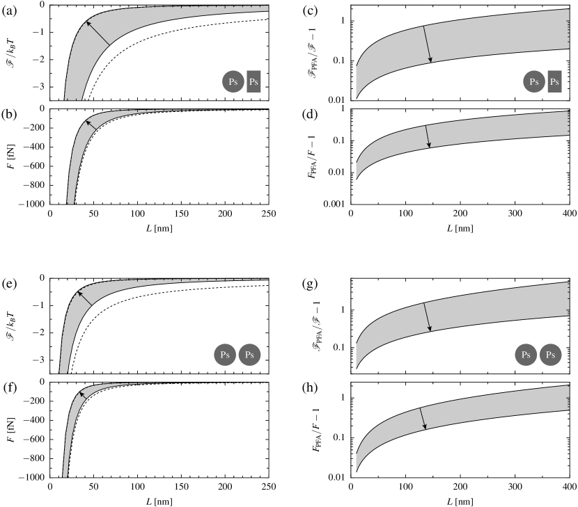
Figure 4: (a) van der Waals free energy and (b) force for a polystyrene sphere with radius $R=1\,\mu\mathrm{m}$ in front of a polystyrene plane in water as a function of the surface-to-surface distance $L$. Solid lines correspond to the numerically exact values and dashed lines to the PFA. The arrow indicates the direction of increasing screening so that the lower curve includes the Matsubara frequency $\xi_{0}$ while the upper curve does not. The grey shaded area indicates the interaction for any intermediate screening strength. The corresponding relative error of the PFA for (c) the van der Waals free energy and (d) force. Here, the upper curve corresponds to the absence of screening and screening increases through the grey area as indicated by the arrow. (e) van der Waals free energy and (f) force for two polystyrene spheres with radii $R_{1}=R_{2}=1\,\mu\mathrm{m}$ in water as a function of the surface-to-surface distance $L$. Corresponding relative error of the PFA for (g) the free energy and (h) the force.

The effective Hamaker parameter for spherical surfaces is determined by Eq. (29) and depends not only on the chosen materials but also on the geometry used in its derivation. Figure 5 demonstrates this dependence for polystyrene and water. The dash-dotted and the solid curves represent the exact effective Hamaker parameter for the plane-sphere and sphere-sphere geometries, respectively, whereas the dashed curve corresponds to the PFA result, which is the same for both geometries. The upper curves do not take screening into account as they include the full contribution from the Matsubara frequency $\xi_{0}.$ In contrast, in the lower curves the Matsubara frequency $\xi_{0}$ is omitted so that these curves correspond to the limit of a vanishingly small Debye screening length: $\lambda_{D}\rightarrow 0.$ For any finite value of $\lambda_{D},$ the Hamaker parameter for each geometry first starts close to the upper curve at short distances ($L\ll\lambda_{D}$) and then is further suppressed by screening, approaching the lower curve for $L\gg\lambda_{D}.$

At small separations, the effective Hamaker parameters derived for the two different geometries asymptotically approach each other and the PFA curve as expected. As the distance increases, the reduction of the effective Hamaker parameter calculated within the PFA accounts for electrodynamical retardation only, whereas the exact curves display an additional reduction associated to curvature. Such geometrical reduction is more apparent in the absence of screening, since in this case the PFA curve at long distances defines a plateau associated to the contribution from the Matsubara frequency $\xi_{0},$ while the exact values decay to zero due to the curvature suppression.

We obtain the value $A=A_{\mathrm{eff}}(L\rightarrow 0)=1.67\,k_{B}T$ for the Hamaker constant. The limiting value is obtained from the short-distance plateau defined by the upper curves in Fig. 5 since they correspond to $L\ll\lambda_{D}.$ On the other hand, the short-distance plateau associated to the lower curves yields the value $0.90\,k_{B}T,$ representing the difference between the Hamaker constant and the contribution from the Matsubara frequency $\xi_{0},$ which in turn corresponds to the long-distance plateau defined by the upper PFA curve in Fig. 5. Our value for $A$ is about half of the theoretical value found in the literature.Russel1989 This is because the optical data in Ref. Zwol2010, used here differ from Parsegian’s optical data set.Parsegian2005 It is interesting to observe that even though the difference between the permittivities of the two data sets is small, namely less than 10%, the difference for the resulting Hamaker constants can be much bigger. This is because, at least within the PFA, the permittivities of the objects and the medium enter in terms of their differences. For polystyrene and water, the optical data almost match for UV frequencies. These frequencies become more and more important as the distance between the surfaces decreases, and then small differences in the optical data can result in relatively large differences in the Hamaker constant. The reduction of the Hamaker constant observed in the experiment of Ref. Wodka2014, could hence be partly due to uncertainties of the optical data.

Figure 5: Effective Hamaker parameter for two polystyrene objects in water as a function of the surface-to-surface distance $L$. The dash-dotted and solid lines are derived from the exact plane-sphere and sphere-sphere interaction forces, respectively. The dashed line is computed within the PFA and is the same for both geometries. The radius of the sphere(s) is $1\,\mathrm{\mu m}$. The arrow indicates the direction of increasing screening strength with the upper (lower) curve including (excluding) the Matsubara frequency $\xi_{0}$.

IV.2 Mercury and polystyrene in water

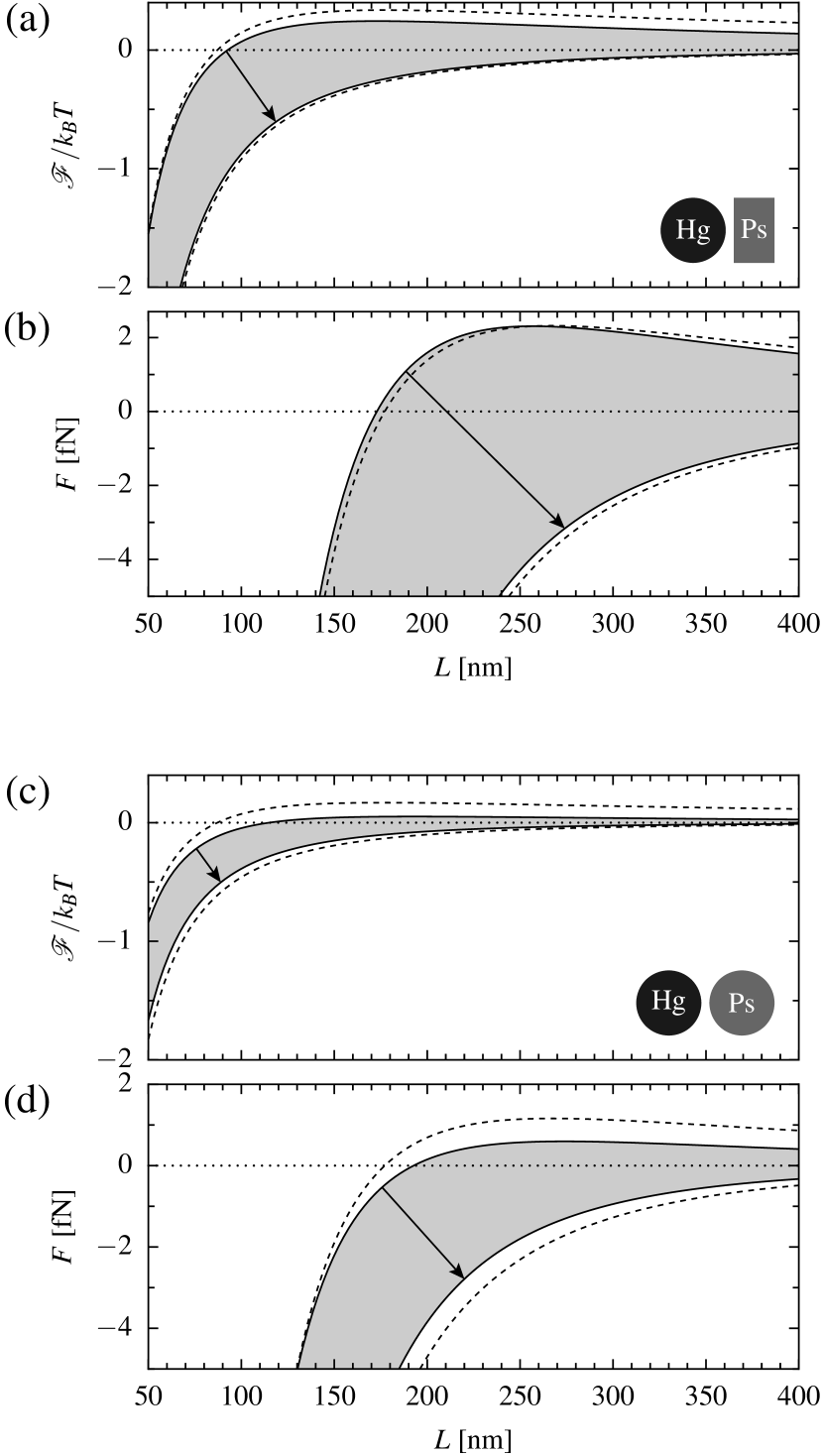
Figure 6: (a) van der Waals free energy and (b) force between a mercury sphere of radius $R=1\,\mu\mathrm{m}$ and a polystyrene plane in water. (c) van der Waals free energy and (d) force between a mercury sphere and a polystyrene sphere with radii $R_{1}=R_{2}=1\,\mu\mathrm{m}$ in water. For both scattering geometries, the quantities are presented as a function of the surface-to-surface distance $L$. The solid lines correspond to the numerically exact results and the dashed lines to the PFA. A positive (negative) sign of the force represents repulsion (attraction). The arrows indicate the direction of increasing screening strength with the upper (lower) curve including (excluding) the Matsubara frequency $\xi_{0}$. The grey shaded area indicates the interaction for any intermediate screening.

Mercury and polystyrene in an aqueous medium constitute an interesting colloid system, since the van der Waals force can be tuned from repulsion to attraction depending on the screening of the zero frequency contribution.Ether2015 Furthermore, due to the high surface tension mercury droplets have a small surface roughness and, thus, corrections due to roughness may play a minor role.Esquivel-Sirvent2014

We study the interaction between a mercury droplet with radius $R=1\,\mathrm{\mu m}$ and a polystyrene wall and the interaction between a mercury droplet with a polystyrene sphere with equal radii $R_{1}=R_{2}=1\,\mathrm{\mu m}$. The dielectric function of mercury is described by the Drude-Smith model Smith2001 with parameters taken from Ref. Esquivel-Sirvent2014, . Figures 6 (a) and (b) depict the van der Waals free energy and force in the plane-sphere geometry, respectively. The corresponding quantities in the sphere-sphere geometry are shown in Figs. 6 (c) and (d).remark Solid lines correspond to the numerically exact results, and the dashed lines to the PFA. We use the convention that a negative sign of the force corresponds to attraction and a positive sign corresponds to repulsion.

When screening is strong, the free energy and the force are negative and monotonic. For negligible screening, both quantities are non-monotonic and can change their sign. At intermediate distances, the force can be tuned from attractive to repulsive depending on the screening strength. Consistent with the discussion of polystyrene in water, the PFA is more accurate in the plane-sphere geometry than in the geometry of two spheres. This becomes most evident when considering the points in which the observables vanish. For instance, according to the PFA the force vanishes at about $L=178\,\mathrm{nm}$ for both geometries. The equilibrium distance is overestimated by about $4\,\mathrm{nm}$ for the plane-sphere geometry and underestimated by about $16\,\mathrm{nm}$ for the two spheres. The determination of the equilibrium distance is particularly relevant for stable equilibria. This is the case for the materials considered in connection with ice particles Thiyam2018 and gas bubbles Esteso2019 in liquid water near a planar interface. Our results suggest that beyond-PFA corrections in the nm range could appear when considering aspect ratios comparable to those taken in Fig. 6.

Figure 7 shows the effective Hamaker parameter for mercury and polystyrene in water. The effective Hamaker parameter has been computed through the exact force between a sphere and a plane (dash-dotted lines) and the exact force between two spheres (solid lines). We also show the results obtained within the PFA (dashed lines), which are the same for both geometries. The contribution from the Matsubara frequency $\xi_{0}$ is included in the lower lines but not in the upper ones. For any given Debye screening length, the Hamaker parameter exhibits a crossover from the lower curve to the upper one as the distance increases past $\lambda_{D}.$ We find $A=A_{\mathrm{eff}}(L\rightarrow 0)=5.17\,k_{B}T$ for the Hamaker constant by following the lower short-distance plateau. In this configuration, the contribution $5.81\,k_{B}T$ from non-zero Matsubara frequencies, associated to the short-distance upper plateau, is larger than the Hamaker constant. This is a consequence of the repulsive nature of the contribution from the Matsubara frequency $\xi_{0},$ which corresponds to the negative plateau defined by the lower PFA curve for the longer distances shown in Fig. 7.

Again, the modification of the effective Hamaker parameter associated to the scattering geometry is most pronounced for larger distances provided that screening is negligible. The corresponding exact curves exhibit a non-monotonic behavior as they tend to zero at large distances.

Figure 7: Effective Hamaker parameter for mercury and polystyrene in water as a function of the surface-to-surface distance $L$. The dash-dotted and solid lines are derived from the exact plane-sphere and sphere-sphere interaction forces, respectively. The dashed line is computed within the PFA and is the same for both geometries. The radius of the sphere(s) is $1\,\mathrm{\mu m}$. The arrow indicates the direction of increasing screening strength with the lower (upper) curve including (excluding) the Matsubara frequency $\xi_{0}$.

V Conclusions

A numerical scheme for computing the van der Waals interaction based on the plane-wave representation of the fluctuating electromagnetic modes was proposed. After a Nyström discretization of the plane-wave momenta, the scattering operator becomes a finite matrix and standard linear algebra procedures can be employed. The method is applicable to arbitrary scattering geometries for which the reflection operators of the individual objects are known in the plane-wave basis. It was demonstrated that a rotational symmetry can be exploited by means of a discrete Fourier transform.

The plane-wave numerical method was applied to the plane-sphere and the sphere-sphere geometry. We found that the method converges faster than the common method based on spherical multipoles. By conducting a runtime analysis for the plane-sphere geometry we demonstrated that the new plane-wave method outperforms a state-of-the-art implementation built on spherical multipoles.

For the van der Waals interaction at finite temperatures, the runtime analysis included a comparison of the conventional Matsubara summation with an alternative summation scheme based on a Padé spectrum decomposition. The latter shows an improved convergence rate resulting in a significant speed-up for the computation of the van der Waals interaction at small distances. The plane-wave approach together with the Padé spectrum decomposition put the numerically exact computation of the van der Waals interaction at experimentally relevant distances within reach of standard desktop computers.

As an application, we employed the new method to study the accuracy of the PFA in aqueous colloidal systems. The two extreme cases of very strong and very weak screening were modeled by excluding and including the zero-frequency contribution of the van der Waals interaction, respectively. For polystyrene in water we found that the relative error incurred with the PFA as compared to the numerically exact evaluation is larger than usually anticipated in the literature, especially for low salt concentrations. Moreover, this effect is more pronounced for the interaction of two spheres than for a plane and a sphere. One important consequence is a geometry-dependent reduction of the effective Hamaker parameter as the distance increases, which adds to the reduction effects associated to electrodynamical retardation and screening by ions in solution.

In addition, we studied the van der Waals interaction of a mercury sphere with a polystyrene sphere or a polystyrene wall. These systems have the interesting feature that the interaction force can be tuned from repulsive to attractive as a function of the salt concentration. While for strong screening the force is always attractive, it is repulsive in the case of negligible screening provided the distance between the objects is not too small. In this case, the exact effective Hamaker parameter exhibits a non-monotonic distance dependence that results from a beyond-PFA competition between the repulsive and attractive contributions to the interaction force.

AIP Publishing Data Sharing Policy

The data represented in Figs. 2 to 7 are openly available on Zenodo at http://doi.org/10.5281/zenodo.3751295, cf. Ref. DataAtZenodo, .

Appendix A Polarization transformation coefficients

The coefficients appearing in (9) arise from the transformation between the polarization basis defined with respect to the scattering plane and the TE/TM polarization basis defined with respect to the symmetry axis of the setup. They have been derived in Ref. Spreng2018, and are given by

$$A =\frac{\cos(\Delta\varphi)-\lambdabar_{m}^{4}\big{[}\kappa\kappa^{\prime}+kk^{\prime}\cos(\Delta\varphi)\big{]}\big{[}kk^{\prime}+\kappa\kappa^{\prime}\cos(\Delta\varphi)\big{]}}{1-\lambdabar_{m}^{4}\big{[}\kappa\kappa^{\prime}+kk^{\prime}\cos(\Delta\varphi)\big{]}^{2}}$$ (30)

$$B =-\frac{\lambdabar_{m}^{2}kk^{\prime}\sin^{2}(\Delta\varphi)}{1-\lambdabar_{m}^{4}\big{[}\kappa\kappa^{\prime}+kk^{\prime}\cos(\Delta\varphi)\big{]}^{2}}$$

$$C =\pm\frac{\lambdabar_{m}^{3}[\kappa^{\prime}k^{2}+\kappa kk^{\prime}\cos(\Delta\varphi)]}{1-\lambdabar_{m}^{4}\big{[}\kappa\kappa^{\prime}+kk^{\prime}\cos(\Delta\varphi)\big{]}^{2}}\sin(\Delta\varphi)$$

$$D =\mp\frac{\lambdabar_{m}^{3}[\kappa{k^{\prime}}^{2}+\kappa^{\prime}kk^{\prime}\cos(\varphi)]}{1-\lambdabar_{m}^{4}\big{[}\kappa\kappa^{\prime}+kk^{\prime}\cos(\Delta\varphi)\big{]}^{2}}\sin(\Delta\varphi)\,.$$

Here, $\Delta\varphi=\varphi^{\prime}-\varphi$ and the upper (lower) sign in the coefficients $C$ and $D$ corresponds to an incoming plane wave traveling in positive (negative) $z$-direction.

Appendix B Fresnel coefficients

The reflection at the interface between two homogeneous half spaces filled with a medium and a dielectric material with permittivities $\epsilon_{m}$ and $\epsilon_{d}$, respectively, is described by the Fresnel coefficients BH

$$r_{\mathrm{TE}}(i\xi,\kappa) =\frac{c\kappa-\sqrt{c^{2}\kappa^{2}+\xi^{2}[\epsilon(i\xi)-1]}}{c\kappa+\sqrt{c^{2}\kappa^{2}+\xi^{2}[\epsilon(i\xi)-1]}}\,,$$ (31)

$$r_{\mathrm{TM}}(i\xi,\kappa) =\frac{\epsilon(i\xi)c\kappa-\sqrt{c^{2}\kappa^{2}+\xi^{2}[\epsilon(i\xi)-1]}}{\epsilon(i\xi)c\kappa+\sqrt{c^{2}\kappa^{2}+\xi^{2}[\epsilon(i\xi)-1]}}$$ (32)

with $\epsilon=\epsilon_{d}/\epsilon_{m}$.

Appendix C Padé spectrum decomposition

Integrals containing Bose or Fermi distribution functions can often be transformed into sum-over-poles expressions using Cauchy’s residue theorem. The Padé spectrum decomposition (PSD) is a particularly efficient sum-over-poles scheme,Hu2010 which can also be used for the computation of the van der Waals interaction at finite temperatures. Before explaining the PSD, we outline the more commonly used scheme involving the Matsubara spectrum decomposition (MSD). For simplicity, we restrict the discussion to the van der Waals free energy.

Before using any of the mentioned spectrum decomposition schemes, the van der Waals free energy at temperature $T$ can be expressed in terms of an integral over real frequencies Jaekel1991 ; Genet2000

$$\mathcal{F}=\frac{\hbar}{2\pi}\int_{0}^{\infty}d\omega\,f\left(\frac{\hbar\omega}{k_{B}T}\right)\mathrm{Im}\left[\Phi(\omega)\right]$$ (33)

with

$$\Phi(\omega)=\log\det(1-\mathcal{M}(\omega))$$ (34)

where the round-trip operator $\mathcal{M}$ is defined in Eq. (2). Note that here $\mathcal{M}$ is a function of real frequencies, while in Eq. (1) its argument are imaginary frequencies. For simplicity, we keep the same notation for both operators. The temperature dependence of the van der Waals free energy is captured by the function

$$f(x)=1+2\bar{n}(x)\,,\quad\bar{n}(x)=\frac{1}{e^{x}-1}\,.$$ (35)

Besides quantum fluctuations, the function $f$ accounts for thermal fluctuations through the mean number $\bar{n}$ of photons per mode. It has equally spaced poles along the imaginary axis at the Matsubara frequencies. Using Cauchy’s residue theorem, the van der Waals free energy (33) can be cast into a sum over the imaginary Matsubara frequencies as given in Eq. (1). This procedure has subtleties in connection with the zero-frequency contribution,Guerout2014 which shall not be discussed here further. In numerical applications, the Matsubara sum needs to be truncated and convergence is reached when the number of terms is of the order of $\lambda_{T}/L$ with the thermal wavelength $\lambda_{T}=\hbar c/k_{B}T$.

For the PSD, one starts out by expanding the function $f$ in terms of a Padé approximation,

$$f(x)\approx\frac{2}{x}+2x\frac{P_{N-1}(x^{2})}{Q_{N}(x^{2})}$$ (36)

where $P_{N-1}$ and $Q_{N}$ are polynomials of order $N-1$ and $N$, respectively. Alternatively, $f$ can be expressed in terms of a sum over its simple poles

$$f(x)\approx\frac{2}{x}+1+2\sum_{j=1}^{N}\left(\frac{\eta_{j}}{x+i\xi_{j}}+\frac{\eta_{j}}{x-i\xi_{j}}\right)\,,$$ (37)

where the PSD frequencies $\xi_{j}$ are determined by the roots of $Q_{N}$ and can be computed in terms of eigenvalues of a symmetric tridiagonal matrix. The PSD coefficients $\eta_{j}$ can be calculated recursively as detailed in Ref. Hu2010, . The pole in (37) at $x=0$ remains unchanged with respect to the MSD. Thus, when using the residue theorem, subtleties in connection with the zero-frequency contribution can be treated in the same manner as in the MSD. All other poles now lie unevenly distributed on the imaginary axis.

Figure 8 visualizes the poles at imaginary frequencies $\xi>0$ appearing in (37) as a function of the order $N$ of the Padé approximation. The center of each circle indicates the position of a pole while the area is proportional to the weight of the pole. For sufficiently small frequencies, one observes the regularly spaced poles leading to the Matsubara sum (1). For larger frequencies, the spacing of the poles increases as does their weight. The irregular spacing of the poles implies that the order of the PSD has to be fixed beforehand.

Figure 8: The positive imaginary frequency poles $\xi$ contributing to the Padé spectrum decomposition (PSD) are displayed as a function of the order $N$ of the Padé approximation. The center of the circle indicates the position of the pole while the area of the circle is proportional to the weight associated with the pole.

Within the PSD, the van der Waals free energy is expressed as

$$\mathcal{F}=\frac{k_{B}T}{2}\left[\Phi(0)+2\sum_{j=1}^{N}\eta_{j}\Phi(i\xi_{j})\right]\,.$$ (38)

Careful numerical tests reveal that convergence of the frequency summation is reached quicker when using PSD, since the approximation order scales only as $N\sim\sqrt{\lambda_{T}/L}$. Thus, the PSD is superior to the MSD when computing the van der Waals interaction, in particular for experimentally relevant system parameters.

References

- (1) H.-J. Butt, M. Kappl, Surface and Interfacial Forces (Wiley-VCH, Weinheim, 2010).
- (2) J. N. Israelachvili, Intermolecular and Surface Forces (Academic Press, London, 2011).
- (3) I. E. Dzyaloshinskii , E. M. Lifshitz, L. P. Pitaevskii, “The general theory of van der Waals forces,” Adv. Phys. 10, 165 (1961).
- (4) A. Milling, P. Mulvaney, I. Larson, “Direct Measurement of Repulsive van der Waals Interactions Using an Atomic Force Microscope ,” J. Colloid Interface Sci. 180, 460 (1996).
- (5) J. N. Munday, F. Capasso, V. A. Parsegian, “Measured long-range repulsive Casimir–Lifshitz forces,” Nature 457, 170 (2009).
- (6) R. F. Tabor, R. Manica, D. Y. C. Chan, F. Grieser, R. R. Dagastine, “Repulsive van der Waals Forces in Soft Matter: Why Bubbles Do Not Stick to Walls,” Phys. Rev. Lett. 106, 064501 (2011).
- (7) P. Thiyam, J. Fiedler, S. Y. Buhmann, C. Persson, I. Brevik, M. Boström, D. F. Parsons, “Ice Particles Sink below the Water Surface Due to a Balance of Salt, van der Waals, and Buoyancy Forces," J. Phys. Chem. C 122, 15311 (2018).
- (8) V. Esteso, S. Carretero-Palacios, P. Thiyam, H. Míguez, D. F. Parsons, I. Brevik, M. Boström, “Trapping of Gas Bubbles in Water at a Finite Distance below a Water-Solid Interface," Langmuir 35, 4218 (2019).
- (9) H. B. G. Casimir, “On the attraction between two perfectly conducting plates,” Proc. K. Ned. Akad. Wet. 51, 793 (1948).
- (10) E. M. Lifshitz, “The Theory of Molecular Attractive Forces between Solids,” Sov. Phys. JETP (Engl. Transl.) 2, 73 (1956).
- (11) M. Bordag, G. L. Klimchitskaya, U. Mohideen, and V. M. Mostepanenko, Advances in the Casimir Effect (Oxford University Press, New York, 2009).
- (12) M. A. Bevan, D. C. Prieve, “Direct Measurement of Retarded van der Waals Attraction,” Langmuir 15, 7925 (1999).
- (13) P. M. Hansen, J. K. Dreyer, J. Ferkinghoff-Borg, L. Oddershede, “Novel optical and statistical methods reveal colloid–wall interactions inconsistent with DLVO and Lifshitz theories,” J. Colloid Interface Sci. 287, 561 (2005).
- (14) M. Elzbieciak-Wodka, M. N. Popescu, F. J. Montes Ruiz-Cabello, G. Trefalt, P. Maroni, M. Borkovec, “Measurements of dispersion forces between colloidal latex particles with the atomic force microscope and comparison with Lifshitz theory,” J. Chem. Phys. 140, 104906 (2014).
- (15) D. S. Ether jr., L. B. Pires, S. Umrath, D. Martinez, Y. Ayala, B. Pontes, G. R. de S. Araújo, S. Frases, G.-L. Ingold, F. S. S. Rosa, N. B. Viana, H. M. Nussenzveig, P. A. Maia Neto, “Probing the Casimir force with optical tweezers,” EPL 112, 44001 (2015).
- (16) F. J. Montes Ruiz-Cabello, M. Moazzami-Gudarzi, M. Elzbieciak-Wodka, P. Maroni, “Forces between different latex particles in aqueous electrolyte solutions measured with the colloidal probe technique,” Microsc. Res. Tech. 80, 144 (2017).
- (17) G. L. Klimchitskaya, U. Mohideen, and V. M. Mostepanenko, “The Casimir force between real materials: Experiment and theory,” Rev. Mod. Phys. 81, 1827 (2009).
- (18) R. Decca, V. Aksyuk, and D. López, “Casimir Force in Micro and Nano Electro Mechanical Systems,” Lect. Notes Phys. 834, 287 (2011).
- (19) S. K. Lamoreaux, “Progress in Experimental Measurements of the Surface–Surface Casimir Force: Electrostatic Calibrations and Limitations to Accuracy,” Lect. Notes Phys. 834, 219 (2011).
- (20) G. L. Klimchitskaya, V. M. Mostepanenko, “Recent measurements of the Casimir force: Comparison between experiment and theory,” Mod. Phys. Lett. A 35, 2040007 (2020).
- (21) B. Derjaguin, “Untersuchungen über die Reibung und Adhäsion, IV – Theorie des Anhaftens kleiner Teilchen,” Kolloid-Zs. 69, 155 (1934).
- (22) V. A. Parsegian, Van der Waals Forces: A Handbook for Biologists, Chemists, Engineers, and Physicists (Cambridge University Press, Cambridge, 2005).
- (23) B. Spreng, M. Hartmann, V. Henning, P. A. Maia Neto, G.-L. Ingold, “Proximity force approximation and specular reflection: Application of the WKB limit of Mie scattering to the Casimir effect,” Phys. Rev. A 97, 062504 (2018).
- (24) M. Bordag and V. Nikolaev, “Casimir force for a sphere in front of a plane beyond proximity force approximation,” J. Phys. A: Math. Theor. 41, 164002 (2008).
- (25) L. P. Teo, M. Bordag, and V. Nikolaev, “Corrections beyond the proximity force approximation,” Phys. Rev. D 84, 125037 (2011).
- (26) L. P. Teo, Casimir effect between two spheres at small separations, Phys. Rev. D 85, 045027 (2012).
- (27) L. P. Teo, “Material dependence of Casimir interaction between a sphere and a plate: First analytic correction beyond proximity force approximation,” Phys. Rev. D 88, 045019 (2013).
- (28) V. Henning, B. Spreng, M. Hartmann, G.-L. Ingold, P. A. Maia Neto, “Role of diffraction in the Casimir effect beyond the proximity force approximation,” J. Opt. Soc. Am. B 36, C77 (2019).
- (29) C. D. Fosco, F. C. Lombardo, and F. D. Mazzitelli, “Proximity force approximation for the Casimir energy as a derivative expansion,” Phys. Rev. D 84, 105031 (2011).
- (30) G. Bimonte, T. Emig, R. L. Jaffe, and M. Kardar, “Casimir forces beyond the proximity approximation,” EPL 97, 50001 (2012).
- (31) G. Bimonte, T. Emig, and M. Kardar, “Material dependence of Casimir forces: Gradient expansion beyond proximity,” Appl. Phys. Lett.. 100, 074110 (2012).
- (32) C. D. Fosco, F. C. Lombardo, and F. D. Mazzitelli, Derivative-expansion approach to the interaction between close surfaces, Phys. Rev. A 89, 062120 (2014).
- (33) C. D. Fosco, F. C. Lombardo, and F. D. Mazzitelli, “Derivative expansion for the electromagnetic Casimir free energy at high temperatures,” Phys. Rev. D 92, 125007 (2015).
- (34) G. Bimonte, “Beyond-proximity-force-approximation Casimir force between two spheres at finite temperature” Phys. Rev. D 97, 085011 (2018).
- (35) G. Bimonte, “Beyond-proximity-force-approximation Casimir force between two spheres at finite temperature. II. Plasma versus Drude modeling, grounded versus isolated spheres,” Phys. Rev. D 98, 105004 (2018).
- (36) M. T. H. Reid, S. G. Johnson, “Efficient Computation of Power, Force, and Torque in BEM Scattering Calculations,” IEEE Trans. Ant. Prop. 63, 3588 (2015).
- (37) A. F. Oskooi, D. Roundy, M. Ibanesca, P. Bermel, J. D. Joannopoulos, S. G. Johnson, “Meep: A flexible free-software package for electromagnetic simulations by the FDTD method,” Comp. Phys. Comm. 181, 687 (2010).
- (38) A. Lambrecht, P. A. Maia Neto, and S. Reynaud, “The Casimir effect within scattering theory,” New J. Phys. 8, 243 (2006).
- (39) T. Emig, N. Graham, R. L. Jaffe, and M. Kardar, “Casimir Forces Between Arbitrary Compact Objects,” Phys. Rev. Lett. 99, 170403 (2007).
- (40) C. P. Boyer, E. G. Kalnins, W. Miller, Jr., “Symmetry and separation of variables for the Helmholtz and Laplace equations,” Nagoya Math. J. 60, 35 (1976).
- (41) G. Bimonte, “Classical Casimir interaction of perfectly conducting sphere and plate,” Phys. Rev. D 95, 065004 (2017).
- (42) P. A. Maia Neto, A. Lambrecht, S. Reynaud, “Casimir energy between a plane and a sphere in electromagnetic vacuum,” Phys. Rev. A 78, 012115 (2008).
- (43) T. Emig, “Fluctuation-induced quantum interactions between compact objects and a plane mirror,” J. Stat. Mech. (2008) P04007.
- (44) A. Canaguier-Durand, P. A. Maia Neto, A. Lambrecht, S. Reynaud, “Thermal Casimir Effect for Drude metals in the plane-sphere geometry,” Phys. Rev. A 82, 012511 (2010).
- (45) A. Canaguier-Durand, “Multipolar scattering expansion for the Casimir effect in the sphere-plane geometry,” Ph.D. thesis (Université Pierre et Marie Curie, 2011).
- (46) A. Canaguier-Durand, G.-L. Ingold, M.-T. Jaekel, A. Lambrecht, P. A. Maia Neto, S. Reynaud, “Classical Casimir interaction in the plane-sphere geometry,” Phys. Rev. A 85, 052501 (2012).
- (47) S. Umrath, M. Hartmann, G.-L. Ingold, P. A. Maia Neto “Disentangling geometric and dissipative origins of negative Casimir entropies,” Phys. Rev. E 92, 042125 (2015).
- (48) R. Messina, P. A. Maia Neto, B. Guizal, M. Antezza, “Casimir interaction between a sphere and a grating,” Phys. Rev. A 92, 062504 (2015).
- (49) M. Hartmann, G.-L. Ingold, and P. A. Maia Neto, “Plasma versus Drude Modeling of the Casimir Force: Beyond the Proximity Force Approximation,” Phys. Rev. Lett. 119, 043901 (2017).
- (50) M. Hartmann, G.-L. Ingold, P. A. Maia Neto, “Advancing numerics for the Casimir effect to experimentally relevant aspect ratios,” Phys. Scr. 93, 114003 (2018).
- (51) M. Hartmann, “Casimir effect in the plane-sphere geometry: Beyond the proximity force approximation,” Ph.D. thesis (Universität Augsburg, 2018).
- (52) H. C. van de Hulst, Light scattering by small particles (Wiley, New York, 1957).
- (53) S. N. Thennadil, L. H. Garcia-Rubio, “Approximations for Calculating van der Waals Interaction Energy between Spherical Particles–A Comparison,” J. Colloid Interface Sci. 243, 136 (2001).
- (54) D. Langbein, “Retarded Dispersion Energy between Macroscopic Bodies,” Phys. Rev. B 2, 3371 (1970).
- (55) D. Langbein, Theory of Van der Waals Attraction (Springer, New York, 1974).
- (56) M. Hartmann, G.-L. Ingold, “CaPS: Casimir Effect in the Plane-Sphere Geometry,” J. Open Source Softw. 5(45), 2011 (2020).
- (57) M. Nieto-Vesperinas, Scattering and Diffraction in Physical Optics (World Scientific, Singapore, 2006).
- (58) F. Bornemann, “On the numerical evaluation of Fredholm determinants,” Math. Comp. 79, 871 (2010).
- (59) K. Kvien, “Angular spectrum representation of fields diffracted by spherical objects: physical properties and implementations of image field models,” J. Opt. Soc. Am. A 15, 636 (1998).
- (60) C. F. Bohren and D. R. Huffman, Absorption and Scattering of Light by Small Particles (Wiley, New York, 1983), Chap. 4.
- (61) H. M. Nussenzveig, “High-Frequency Scattering by a Transparent Sphere. I. Direct Reflection and Transmission,” J. Math. Phys. 10, 82 (1969).
- (62) H. M. Nussenzveig, Diffraction Effects in Semiclassical Scattering (Cambridge University Press, Cambridge, 1992).
- (63) J. P. Boyd, “Exponentially convergent Fourier-Chebshev quadrature schemes on bounded and infinite intervals,” J. Sci. Comp. 2, 99 (1987).
- (64) S. van der Walt, S. C. Colbert, G. Varoquaux, “The NumPy Array: A Structure for Efficient Numerical Computation,” Computing in Science & Engineering 13, 22 (2011).
- (65) P. Virtanen, R. Gommers, T. E. Oliphant et al., “SciPy 1.0: fundamental algorithms for scientific computing in Python,” Nat. Methods 17, 261 (2020).
- (66) S. K. Lam, A. Pitrou, S. Seibert, “Numba: A LLVM-based Python JIT Compiler,” Proceedings of the Second Workshop on the LLVM Compiler Infrastructure in HPC, 7:1 (2015).
- (67) J. Hu, R.-X. Xu, Y. Yan, “Communication: Padé spectrum decomposition of Fermi function and Bose function,” J. Chem. Phys. 133, 101106 (2010).
- (68) H. C. Hamaker, “The London–van der Waals attraction between spherical particles,” Physica 4, 1058 (1937).
- (69) W. B. Russel, D. A. Saville, W. R. Schowalter, Colloidal Dispersions (Cambridge University Press, Cambridge, 1989).
- (70) D. J. Mitchell, P. Richmond, “A general formalism for the calculation of free energies of inhomogeneous dielectric and electrolytic systems,” J. Colloid Interface Sci. 46, 118 (1974).
- (71) J. Mahanty and B. W. Ninham, Dispersion Forces (Academic Press, London, 1976).
- (72) P. A. Maia Neto, F. S. S. Rosa, L. B. Pires, A. B. Moraes, A. Canaguier-Durand, R. Guérout, A. Lambrecht, S. Reynaud, “Scattering theory of the screened Casimir interaction in electrolytes,” Eur. Phys. J. D 73, 178 (2019).
- (73) P. J. van Zwol, G. Palasantzas, “Repulsive Casimir forces between solid materials with high-refractive-index intervening liquids,” Phys. Rev. A 81, 062502 (2010).
- (74) B. A. Pailthorpe, W. B. Russel, “The retarded van der Waals interaction between spheres,” J. Colloid Interface Sci. 89, 563 (1982).
- (75) R. Esquivel-Sirvent, J. V. Escobar, “Casimir force between liquid metals,” EPL 107, 40004 (2014).
- (76) N. V. Smith, “Classical generalization of the Drude formula for the optical conductivity,” Phys. Rev. B 64, 155106 (2001).
- (77) Such calculations have been performed before in Ref. Ether2015, . An implementation error affecting the Gaunt coefficient at large orders, however, lead to erroneous results for the Casimir force for small separations which were corrected in Ref. Umrath2016, .
- (78) B. Spreng, P. A. Maia Neto, G.-L. Ingold (2020). “Data for "Plane-wave approach to the exact van der Waals interaction for colloid particles",” Zenodo. http://doi.org/10.5281/zenodo.3751295
- (79) M. T. Jaekel and S. Reynaud, “Casimir force between partially transmitting mirrors,” J. Phys. I France 1, 1395 (1991).
- (80) C. Genet, A. Lambrecht, S. Reynaud, “Temperature dependence of the Casimir effect between metallic mirrors,” Phys. Rev. A 62, 012110 (2000).
- (81) R. Guérout, A. Lambrecht, K. A. Milton, S. Reynaud, “Derivation of the Lifshitz-Matsubara sum formula for the Casimir pressure between metallic plane mirrors,” Phys. Rev. E 90, 042125 (2014).
- (82) S. Umrath, “Der Casimir-Effekt in der Kugel-Kugel-Geometrie: Theorie und Anwendung auf das Experiment,” Ph.D. thesis (Universität Augsburg, 2016).