Tuning photon statistics with coherent fields

Abstract

Photon correlations, as measured by Glauber’s $n$-th order coherence functions $g^{(n)}$, are highly sought to be minimized and/or maximized. In systems that are coherently driven, so-called blockades can give rise to strong correlations according to two scenarios based on level-repulsion (conventional blockade) or interferences (unconventional blockade). Here we show how these two approaches relate to the admixing of a coherent state with a quantum state such as a squeezed state for the simplest and most recurrent case. The emission from a variety of systems, such as resonance fluorescence, the Jaynes–Cummings model or microcavity polaritons, as a few examples of a large family of quantum optical sources, are shown to be particular cases of such admixtures, that can further be doctored-up externally by adding an amplitude- and phase-controlled coherent field with the effect of tuning the photon statistics from exactly zero to infinity. We show how such an understanding also allows to classify photon statistics throughout platforms according to conventional and unconventional features, with the effect of optimizing the correlations and with possible spectroscopic applications. In particular, we show how configurations that can realize simultaneously conventional and unconventional antibunching bring the best of both worlds: huge antibunching (unconventional) with large populations and being robust to dephasing (conventional).

I Introduction

That the sum (or superposition) of two fields does not simply add their respective intensities but introduce an interference term is the basic principle of optics and other wave theories Young (1807). In this text, we study the impact that such interferences have on the quantum-optical aspect of light. Since quantum optics typically deals with correlations between photons, our concern is primarily with the photon statistics of interfering fields Ficek and Swain (2004). The effect of interferences on photon statistics has been previously studied in the literature, both past and recent Ritze and Bandilla (1979); Paul (1982); Bužek and Knight (1995); Prakash and Mishra (2005); Majumdar et al. (2012); Boddeda et al. (2019) but its ubiquity in a wealth of physical systems has been greatly overlooked. In particular, it appears to be central in coherently-driven systems, even when one is not directly controlling the phase and amplitude of the coherent field with the aim of interfering it with its quantum counterpart. The problem was first considered in this form by Vogel Vogel (1991, 1995) to bring to the quantum realm the signal-engineering technique of homodyning, namely, to extract squeezing (rather than phase modulation in the classical case). In fact, a related case when the coherent field interferes with a quantum field that it generates as the result of driving a quantum emitter, had been previously introduced by Carmichael under the apt denomination of “self-homodyning” Carmichael (1985). The technique has been lately championed in a recent series of works from the Vuc̆ković group Fischer et al. (2016); Müller et al. (2016); Dory et al. (2017); Fischer et al. (2017, 2018) and a recent work controlled the interference to tune the photon statistics Foster et al. (2019). The problem is so widespread, often in disguise, that even a brief overview of its occurrences and its identification throughout platforms and realizations, takes the character of a self-contained Review Zubizarreta Casalengua et al. (2020), to which we refer for further discussion of the literature. Here, we consider mainly the case of mixing a squeezed state with a coherent field, as this is the most common configuration, although the general case is clearly also of fundamental interest Lvovsky and Babichev (2002); Windhager et al. (2011); Xu et al. (2012); Mehringer et al. (2018).

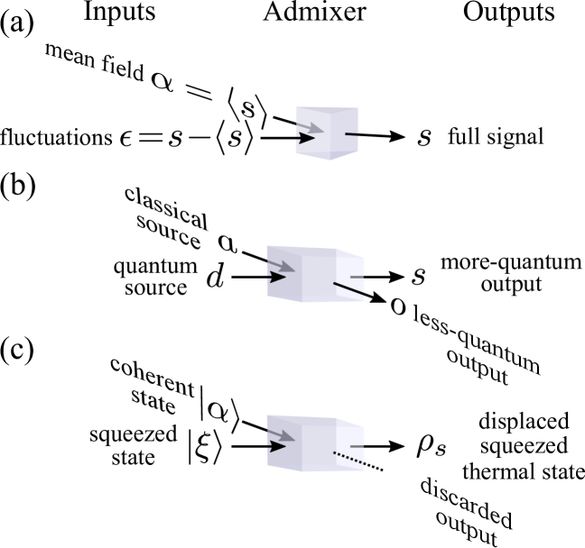
Figure 1: Schemes considered in this text. (a) A quantum field $s$ can be seen as composed of a classical component (its mean field) $\langle s\rangle$ and quantum fluctuations $\epsilon$. (b) By using a beam splitter, a classical source $a$ can be used to remove the classical component from a quantum source $d$ resulting in a more quantum output $s$. The excess of classical signal is redirected towards the other branch of the interferometer in $o$. (c) A particular case of great popularity in the literature admixes a coherent state $\ket{\alpha}$ to a squeezed state $\ket{\xi}$, producing a displaced squeezed thermal state in a density matrix form $\rho_{s}$ as the other output is discarded (traced over).

II Homodyning a quantum field.

A simple but powerful decomposition in quantum field theory separates the mean field $\alpha\equiv\langle s\rangle$ from the quantum fluctuations $\epsilon\equiv s-\langle s\rangle$ of a quantum field $s$, which is recovered by bringing these two components together Blaizot and Ripka (1985):

$$s=\alpha+\epsilon\,.$$ (1)

Note that $\epsilon$, like $s$, is an operator, and thus describes a quantum field. In contrast, $\alpha$ is a $c$ number, and describes a classical field. This decomposition is sketched in Fig. 1(a). This trivial mathematical fact, to which theorists recourse to treat the two components separately, can be in essence realized in a physical setting for instance by using a beam splitter, i.e., a two-inputs ($a$, $d$), two-outputs ($o$, $s$) linear and unitary transformation which, for optical fields, and assuming a transmittance $\mathrm{T}^{2}$ and reflectance $\mathrm{R}^{2}$, reads as Gerry and Knight (2005):

$$\begin{pmatrix}o\\ s\end{pmatrix}=\begin{pmatrix}i\mathrm{R}&\mathrm{T}\\ \mathrm{T}&i\mathrm{R}\end{pmatrix}\begin{pmatrix}d\\ a\end{pmatrix}$$ (2)

with $0\leq\mathrm{T},\mathrm{R}\leq 1$ and $\mathrm{T}^{2}+\mathrm{R}^{2}=1$. The $i$ term comes from Stokes’ relations and can be corrected with a half-wave plate, so that, assuming a balanced beam-splitter $\mathrm{R}=\mathrm{T}=1/\sqrt{2}$, we can have $o=(i/\sqrt{2})(-a+d)$ and $s={1/\sqrt{2}}(a+d)$, with the outputs providing an attenuated fraction of the difference and sum of the two input fields. The phase shift in the difference could also be removed with another half-wave plate. The attenuation comes from energy-conservation and the impossibility to amplify faithfully a quantum field. Since one can, however, amplify faithfully a classical field, then an amplification by a factor $\mathrm{T}/\mathrm{R}$, together with the half-wave plate phase shift of $-i$ and passing through an unbalanced beam splitter, returns on the transmitted output the signal $s=T(a+d)$ and on the reflected one $o=i[\mathrm{R}d-(\mathrm{T}^{2}/\mathrm{R})a]$. Therefore, in the limit $\mathrm{T}\rightarrow 1$, which is theoretical only since this requires infinite amplification, one can recover the sum of the two fields without attenuation, $s=a+d$. The other field then collects the diverging (due to amplification) classical field alone $-i(\mathrm{T}/\mathrm{R})\langle\sigma\rangle$. As this classical field can be discarded without affecting the quantum field, this hypothetical setup realizes the scheme sketched in Fig. 1(a) by feeding it with the quantum fluctuations $d=\epsilon$ and the mean-field $a=\langle s\rangle$. In the following, we will exploit such decompositions as Eq. (1) as well as the possibility to interfere in a beam splitter a classical source $a$ with a quantum source $d$, to similarly collect on the one hand the magnified quantum character of the quantum source, that is, devoid of its mean field, that is re-routed, on the other hand, in another channel which can be traced over. This is sketched in Fig. 1(b). We have shown for instance how one can collect in this way the pure quantum emission from a coherently driven two-level system by destructively interfering its mean-field López Carreño et al. (2018). We now generalize this scheme to other quantum sources.

Being interested in the $s$ component alone, and in particular in its quantum averages, to describe the beam-splitter situation, we perform a binomial expansion on $s=\mathrm{T}d+i\mathrm{R}a$ and its conjugate to compute

$$\langle s^{\dagger n}s^{m}\rangle=T^{n+m}\\ \sum_{p=0}^{n}\sum_{q=0}^{m}\binom{n}{p}\binom{m}{q}i^{q-p}(\mathrm{R}/\mathrm{T})^{p+q}\langle a^{\dagger p}a^{q}d^{\dagger(n-p)}d^{m-p}\rangle$$ (3)

which includes the beam-splitting signal reduction as well as the $\pi$ phase-shift for reflection. While those will typically be present in an actual experiment, they are not so important for the actual process of interfering (or mixing) the fields and can be absorbed in an overall leading factor which will, in fact, cancel in all normalized correlators. This reflects the fact that photon statistics is not affected by linear processes. In this case, one can consider directly the correlators that arise from the simple addition of the fields $s=a+d$:

$$\langle s^{\dagger n}s^{m}\rangle=\sum_{p=0}^{n}\sum_{q=0}^{m}\binom{n}{p}\binom{m}{q}\langle a^{\dagger p}a^{q}d^{\dagger(n-p)}d^{m-p}\rangle\,.$$ (4)

Besides, one can assume no correlations between the two inputs, so that $\langle a^{\dagger p}a^{q}d^{\dagger(n-p)}d^{m-p}\rangle=\langle a^{\dagger p}a^{q}\rangle\langle d^{\dagger(n-p)}d^{m-p}\rangle$ and since we presently concern ourselves with the case where $a$ is classical, i.e., with $\alpha=\langle a\rangle$, we can further simplify Eq. (4) into

$$\langle s^{\dagger n}s^{m}\rangle=\sum_{p=0}^{n}\sum_{q=0}^{m}\binom{n}{p}\binom{m}{q}\alpha^{*p}\alpha^{q}\langle d^{\dagger(n-p)}d^{m-q}\rangle\,.$$ (5)

This yields, as the simplest ($n=m=1$) case, the classical version of interfering fields, that holds at the one-photon level (in the sense of first-order correlations). Namely, the output field $s$ sums the intensities of the two fields, plus or minus an interfering term:

$$\langle n_{s}\rangle\equiv\langle{s^{\dagger}}s\rangle=|\alpha|^{2}+\langle n_{d}\rangle+2\mathrm{Re}[\alpha^{*}\langle d\rangle]\,.$$ (6)

So far this is just a sophisticated way to write one of the most basic and best known features of optics: interferences. One departs from the classical realm in the next orders, with $n=m\geq 2$. Correlations are typically normalized, which yields the $n$th-order photon correlation $g^{(n)}\equiv{\langle s^{\dagger n}s^{n}\rangle}/{\langle n_{s}\rangle^{n}}$ Glauber (1963) that one can write in increasing powers of $\alpha$, namely,

$$g^{(2)}_{s} =1+\mathcal{I}_{0}+\mathcal{I}_{1}+\mathcal{I}_{2}\,,$$ (7a)

$$g^{(3)}_{s} =1+\mathcal{J}_{0}+\mathcal{J}_{1}+\mathcal{J}_{2}+\mathcal{J}_{3}+\mathcal{J}_{4}\,,$$ (7b)

$$g^{(k)}_{s} =1+\sum_{m=0}^{2n-2}\mathcal{K}_{m}\,,$$ (7c)

with $\mathcal{I}_{m}\langle n_{s}\rangle^{2}$, $\mathcal{J}_{m}\langle n_{s}\rangle^{3}$, $\mathcal{K}_{m}\langle n_{s}\rangle^{4}\propto|\alpha|^{m}$. Note that there are no explicit terms $\mathcal{K}_{2n-1}$, $\mathcal{K}_{2n}$ (e.g., $\mathcal{I}_{3}$, $\mathcal{I}_{4}$ for $g^{(2)}$ and $\mathcal{J}_{5},\mathcal{J}_{6}$ for $g^{(3)}$) because, through simplifications, these get absorbed in the unit term 1, which otherwise comes from the coherent field. The non-coherent (quantum) contributions read as, for $g^{(2)}$ Mandel (1982); Carmichael (1985); Vogel (1991, 1995),

$$\mathcal{I}_{0} =\frac{\langle d^{\dagger 2}d^{2}\rangle-\langle{d^{\dagger}}d\rangle^{2}}{\langle n_{s}\rangle^{2}}\,,$$ (8a)

$$\mathcal{I}_{1} =4\frac{\mathrm{Re}[\alpha^{*}(\langle{d^{\dagger}}d^{2}\rangle-\langle{d^{\dagger}}d\rangle\langle d\rangle)]}{\langle n_{s}\rangle^{2}}\,,$$ (8b)

$$\mathcal{I}_{2} =2\frac{\mathrm{Re}[{\alpha^{*}}^{2}\langle d^{2}\rangle]-2\mathrm{Re}[\alpha^{*}\langle d\rangle]^{2}+|\alpha|^{2}\langle{d^{\dagger}}d\rangle}{\langle n_{s}\rangle^{2}}$$ (8c)

and, for $g^{(3)}$,

$$\mathcal{J}_{0} =\frac{\langle d^{\dagger 3}d^{3}\rangle-\langle{d^{\dagger}}d\rangle^{3}}{\langle n_{s}\rangle^{3}}\,,$$ (9a)

$$\mathcal{J}_{1} =6\frac{\mathrm{Re}[\alpha^{*}\left(\langle d^{\dagger 2}d^{3}\rangle-\langle d\rangle\langle{d^{\dagger}}d\rangle\right)]}{\langle n_{s}\rangle^{3}}\,,$$ (9b)

$$\mathcal{J}_{2} =3\Big{[}2\mathrm{Re}[{\alpha^{*}}^{2}\langle{d^{\dagger}}d^{3}\rangle]+|\alpha|^{2}\left(3\langle d^{\dagger 2}d^{2}\rangle+\langle{d^{\dagger}}d\rangle^{2}\right)$$

$$\hskip 99.58464pt-4\langle{d^{\dagger}}d\rangle\mathrm{Re}[\alpha^{*}\langle d\rangle]^{2}\Big{]}/\langle n_{s}\rangle^{3}\,,$$ (9c)

$$\mathcal{J}_{3} =2\Big{[}\mathrm{Re}[{\alpha^{*}}^{3}\langle d^{3}\rangle]+|\alpha|^{2}\mathrm{Re}[\alpha^{*}\left(9\langle{d^{\dagger}}d^{2}\rangle-6\langle d\rangle\langle{d^{\dagger}}d\rangle\right)]$$

$$\hskip 99.58464pt-4\mathrm{Re}[\alpha^{*}\langle d\rangle]^{3}\Big{]}/\langle n_{s}\rangle^{3}\,,$$ (9d)

$$\mathcal{J}_{4} =6|\alpha|^{2}\frac{\mathrm{Re}[{\alpha^{*}}^{2}\langle d^{2}\rangle]+|\alpha|^{2}\langle{d^{\dagger}}d\rangle-2\mathrm{Re}[\alpha^{*}\langle d\rangle]^{2}}{\langle n_{s}\rangle^{3}}\,.$$ (9e)

It is possible, though not necessary presently, to provide the higher-order-correlators terms $\mathcal{K}_{m}$. In connection of our coming discussion on squeezing, note that $\mathcal{I}_{2}$ can be rewritten in terms of the field quadratures:

$$\mathcal{I}_{2}=4\Big{[}|\alpha|^{2}\left(\cos^{2}\phi\ \langle{:}X_{d}^{2}{:}\rangle+\sin^{2}\phi\ \langle{:}Y_{d}^{2}{:}\rangle+{}\right.\\ \quad\left.{}+\cos\phi\sin\phi\ \langle\{X_{d},Y_{d}\}\rangle\right)-\mathrm{Re}[\alpha^{*}\langle d\rangle]^{2}\Big{]}/\langle n_{s}\rangle^{2}\,.$$ (10)

Here, the notation “$::$” indicates normal ordering, $\{X_{d},Y_{d}\}\equiv X_{d}Y_{d}+Y_{d}X_{d}$, and $X_{d}\equiv\frac{1}{2}\left({d^{\dagger}}+d\right)$, $Y_{d}\equiv\frac{i}{2}\left({d^{\dagger}}-d\right)$ are the quadratures of the field described with the annihilation operator $d$. Such decompositions of the photon statistics, [Eqs. (7)], pinpoint which mechanism is at play in accounting for the photon correlations. The coefficients $\mathcal{I}_{0}$ and $\mathcal{J}_{0}$, for instance, quantify the statistics of the quantum part of the signal, and through the first term in the numerator, are basically the Glauber correlators themselves. $\mathcal{I}_{0}$ also bears some resemblance to Mandel’s $Q$ parameter Mandel (1979). Indeed, when there is no coherence involved and the full signal is quantum, i.e., when $s\approx d$, then $\mathcal{I}_{0}=g^{(2)}-1$ and $\mathcal{J}_{0}=g^{(3)}-1$ (and similarly at still higher orders) with all other $\mathcal{I}_{k}$, $\mathcal{J}_{k}$ cancelling. In this case, the photon statistics can be fully attributed to the quantum dynamics of the naked emitter. In other cases, it includes interferences with the coherent contribution, which are the multi-photon counterpart for the photon statistics of the usual field (single-photon) interference, [Eq. 6], for intensities. At the two-photon level, $\mathcal{I}_{2}$ shows that the interference can be well described through squeezing of the quantum signal, and we will study exactly this configuration in the next section. At the three-photon level, the situation becomes more complex with departures from the exact squeezed and coherent-states interference scenario Zubizarreta Casalengua et al. (2020), and we will therefore focus on the simpler, and so far more popular, case of two-photon statistics. Nevertheless, the same underlying idea of multiphoton interferences prevails.

We conclude this section with the version of Eqs. (8) which will be used in the rest of the text, where we shall consider both the cases where the coherent state is brought externally to the emitter (homodyning) and the case where the coherent state is the classical, or mean-field, component of the emitter itself (self-homodyning). In the latter case, coming back to Eq. (1), with $d=\epsilon=s-\langle s\rangle$ and $a=\langle s\rangle$, one finds for the $\mathcal{I}$ coefficients (the same could be done for $\mathcal{J}$, etc.):

$$\mathcal{I}_{0} =\Big{[}{\langle s^{\dagger 2}s^{2}\rangle-\langle{s^{\dagger}}s\rangle^{2}-4|\langle s\rangle|^{4}+6|\langle s\rangle|^{2}\langle{s^{\dagger}}s\rangle}+{}$$

$$\kern 28.45274pt{2\mathrm{Re}[{\langle{s^{\dagger}}\rangle}^{2}\langle s^{2}\rangle-2\langle{s^{\dagger}}\rangle\langle{s^{\dagger}}s^{2}\rangle]}\Big{]}/{\langle{s^{\dagger}}s\rangle^{2}}\,,$$ (11a)

$$\mathcal{I}_{1} =4\frac{\mathrm{Re}[\langle{s^{\dagger}}\rangle\langle{s^{\dagger}}s^{2}\rangle-\langle{s^{\dagger}}\rangle^{2}\langle s^{2}\rangle]+2|\langle s\rangle|^{2}\left(|\langle s\rangle|^{2}-\langle{s^{\dagger}}s\rangle\right)}{\langle{s^{\dagger}}s\rangle^{2}}\,,$$ (11b)

$$\mathcal{I}_{2} =2\frac{\mathrm{Re}[\langle{s^{\dagger}}\rangle^{2}\langle s^{2}\rangle]+|\langle s\rangle|^{2}\langle{s^{\dagger}}s\rangle-2|\langle s\rangle|^{4}}{\langle{s^{\dagger}}s\rangle^{2}}\,.$$ (11c)

III Interfering a squeezed and a coherent state

We now focus on one case of considerable interest, as it is possibly the most recurring case, although not always identified as such, namely, when the quantum state is a squeezed state. Note that a squeezed state has a zero mean, $\langle d\rangle=0$, so it technically qualifies as a fluctuation term in the sense of Eq. (1). However, since it can be the dominant term of the total population, we will also refer to it as the quantum part of the signal. The operators $a$ and $d$ are now both annihilation operators for bosonic fields, and we define $D_{a}(\alpha)\equiv\exp(\alpha{a^{\dagger}}-\alpha^{\ast}a)$ the displacement operator for the coherent state $\ket{\alpha}=D_{a}(\alpha)\ket{0}$, with $\alpha=|\alpha|e^{i\phi}$ and $S_{d}(\xi)\equiv\exp({1\over 2}[\xi d^{\dagger\,2}-\xi^{\ast}d^{2}])$ the squeezing operator for the squeezed state $\ket{\xi}=S_{d}(\xi)\ket{0}$, with $\xi=re^{i\theta}$ the squeezing parameter. The total input state is then

$$\ket{\psi_{\mathrm{in}}}={D}_{a}\left(\alpha\right){S}_{d}\left(\xi\right)\ket{0}_{da},$$ (12)

where the state subscript indicates the input and output subspaces where operators are acting upon, namely, here, in the input basis. Now, applying the transformation Eq. (2) and rearranging terms, we obtain, first for the displacement operator, ${D}_{a}\left(\alpha\right)=\exp\left(\alpha_{o}{o^{\dagger}}-\alpha_{o}^{*}o+\alpha_{s}{s^{\dagger}}-\alpha_{s}^{*}s\right)$, where $\alpha_{s}=i\mathrm{R}\alpha$ and $\alpha_{o}=\mathrm{T}\alpha$. Exponentials of operators can be factorized since both outputs are independent from each other and commute. This leads to $D_{a}\left(\alpha\right)=D_{o}\left(\alpha_{o}\right)D_{s}\left(\alpha_{s}\right)=D_{s}\left(\alpha_{s}\right)D_{o}\left(\alpha_{o}\right)$, where each displacement operator $D_{j}\left(\alpha_{j}\right)$ ($j=o,s$) only acts over its assigned output. Second, the squeezing operator in the output basis reads as

$${S}_{d}\left(\xi\right)=\exp\left[\frac{1}{2}\left(\xi_{o}^{*}o^{2}-\xi_{o}{o^{\dagger}}\right)+\frac{1}{2}\left(\xi_{s}^{*}s^{2}-\xi_{s}{s^{\dagger}}\right)+\right.\\ \left.\left(\xi_{os}^{*}os-\xi_{os}{o^{\dagger}}{s^{\dagger}}\right)\right]=\exp(S_{o}+S_{s}+S_{os})\,,$$ (13)

where $\xi_{s}=\mathrm{T}^{2}\xi$, $\xi_{o}=-\mathrm{R}^{2}\xi$ and $\xi_{os}=i\mathrm{R}\mathrm{T}\,\xi$. This exponential can be split into a product, only if $[S_{o}+S_{s},S_{os}]=0$, which is fulfilled in the particular case of a balanced BS, $\mathrm{T}=\mathrm{R}$. This restriction is however not very stringent since its first-order correction grows proportionally to $r^{2}\mathrm{T}\mathrm{R}\left(\mathrm{T}^{2}-\mathrm{R}^{2}\right)$. Thus, for either low squeezing signal ($r\ll 1$) or almost symmetrical BS ($\mathrm{T}-\mathrm{R}\approx 0$), the output signal can still be described as follows. Since the commutator $[S_{o},S_{s}]$ vanishes for all possible values, the exponential simplifies into $S_{d}\left(\xi\right)=S_{o}\left(\xi_{o}\right)S_{s}\left(\xi_{s}\right)S_{os}\left(\xi_{os}\right)$. Therefore, the output state can be written as

$$\ket{\psi_{\mathrm{out}}}=D_{o}\left(\alpha_{o}\right)S_{o}\left(\xi_{o}\right)D_{s}\left(\alpha_{s}\right)S_{s}\left(\xi_{s}\right)S_{os}\left(\xi_{os}\right)\ket{0}_{os}\\ =D_{o}\left(\alpha_{o}\right)S_{o}\left(\xi_{o}\right)D_{s}\left(\alpha_{s}\right)S_{s}\left(\xi_{s}\right)\ket{\xi_{os}}_{os},$$ (14)

where $\ket{\xi_{os}}$ is a two-mode squeezed state, which in the Fock basis reads as Gerry and Knight (2005):

$$\ket{\xi_{os}}=\frac{1}{\cosh r_{os}}\sum_{n=0}^{\infty}\left(\tanh r_{os}\right)^{n}\ket{n,n}_{os},$$ (15)

where $r_{os}=|\xi_{os}|=\mathrm{R}\mathrm{T}\,r$. The corresponding density matrix for this pure state reads as $\rho_{\mathrm{out}}=\ket{\psi_{\mathrm{out}}}\bra{\psi_{\mathrm{out}}}$. Tracing out output $o$, we obtain the density matrix for output $s$ only (our signal of interest): $\rho_{s}=\Tr_{o}\{\rho_{\mathrm{out}}\}$. With the cyclic properties of the trace, we move operators clockwise to act over the output subspace $o$ and use ${D_{o}^{\dagger}}\left(\alpha_{o}\right)D_{o}\left(\alpha_{o}\right)={S_{o}^{\dagger}}\left(\xi_{o}\right)S_{o}\left(\xi_{o}\right)={\mathds{1}}_{o}$, where ${\mathds{1}}_{o}$ is the identity. Furthermore, any operator that only acts on the $s$-subspace can be taken out of the trace. This brings us to an expression for the quantum state of the signal:

$$\rho_{s}=D_{s}\left(\alpha_{s}\right)S_{s}\left(\xi_{s}\right)\big{(}\Tr_{o}\{\ket{\xi_{os}}\bra{\xi_{os}}\}\big{)}{S_{s}^{\dagger}}\left(\xi_{s}\right){D_{s}^{\dagger}}\left(\alpha_{s}\right)\,.$$ (16)

The partial trace $\Tr_{o}\{\ket{\xi_{os}}\bra{\xi_{os}}\}$ has the form of a thermal state

$$\rho_{\mathrm{th}}=\Tr_{o}\{\ket{\xi_{os}}\bra{\xi_{os}}\}=\,\frac{1}{\cosh^{2}r_{os}}\sum_{n}^{\infty}\left(\tanh r_{os}\right)^{2n}\ket{n}_{s}\!\!\bra{n}_{s}$$ (17)

with mean population $\mathrm{p_{th}}\equiv\langle{s^{\dagger}}s\rangle=\sinh^{2}r_{os}$. To sum up, admixing a coherent and a squeezed state as shown in Fig. 1(c) produces on one arm of a beam-splitter a displaced squeezed thermal state Lemonde et al. (2014) where the displacement and squeezing are both in terms of $s=a+d$:

$$\rho_{s}=D_{s}\left(\alpha_{s}\right)S_{s}\left(\xi_{s}\right)\rho_{\mathrm{th}}{S_{s}^{\dagger}}\left(\xi_{s}\right){D_{s}^{\dagger}}\left(\alpha_{s}\right),$$ (18)

with parameters $\alpha_{s}=i\mathrm{R}|\alpha|e^{i\phi}$, $\xi_{s}=r_{s}e^{i\theta_{s}}=\mathrm{R}^{2}e^{i\left(\theta+\pi\right)}$, and $\mathrm{p_{th}}=\sinh[2](\mathrm{R}\mathrm{T}\,r)$. Even though $\mathrm{T}$ and $\mathrm{R}$ appear as free parameters, we remind that Eq. (18) is valid for $\mathrm{R}\approx\mathrm{T}$ (and is exact for $\mathrm{R}=\mathrm{T}$). We now restrict ourselves to the case of a 50:50 beam splitter ($\mathrm{T}^{2}=\mathrm{R}^{2}=1/2$). The thermal population reads as, in terms of the squeezed population of the input signal $\langle n_{d}\rangle=\sinh^{2}r$,

$$\mathrm{p_{\mathrm{th}}}=\frac{1}{2}\left(\sqrt{1+\langle n_{d}\rangle}-1\right)\,.$$ (19)

From $\rho_{s}$ we can compute the observables for the mixed signal:

$$\langle n_{s}\rangle=\frac{|\alpha|^{2}}{2}+\frac{\langle n_{d}\rangle}{2}\,,\quad|\langle s^{2}\rangle|=\left(\mathrm{p_{th}}+\frac{1}{2}\right)\sinh(r)\,,$$ (20a)

$$g^{(2)}_{s}=1+\langle n_{s}\rangle^{-2}\sinh^{2}r\left[\cosh 2r+{}\right.\\ \left.{}+2|\alpha|^{2}\left(1-\cos(\theta-2\phi)\coth r\right)\right]\,,$$ (20b)

$$g^{(3)}_{s}=1+\langle n_{s}\rangle^{-3}\sinh^{2}r\,\Big{\{}\sinh^{2}2r+5\sinh^{2}r\cosh 2r+{}\\ {}+6|\alpha|^{4}\left(1-\cos(\theta-2\phi)\coth r\right)+\\ \>3|\alpha|^{2}\left[3\coth^{2}r-1+6\left(1-\cos(\theta-2\phi)\coth r\right)\right]\Big{\}}\,.$$ (20c)

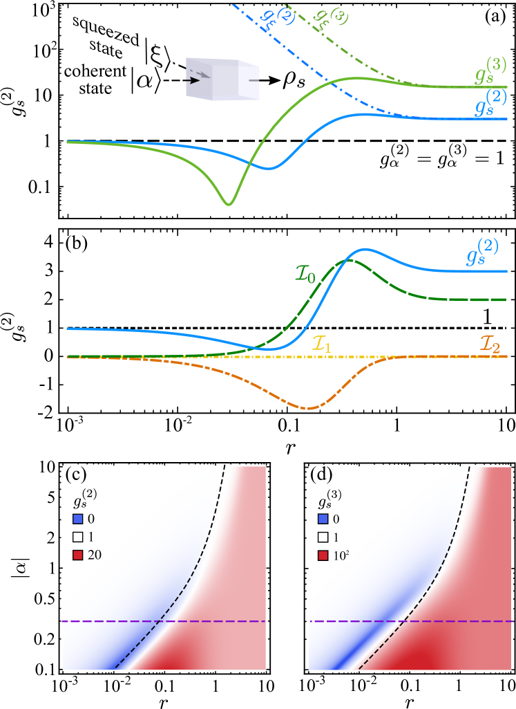
Figure 2: (Color online) (a) Admixing a squeezed state with statistics $g_{\xi}^{(n)}$ (dash-dotted lines, $n=2,3$) with a coherent state with $g_{\alpha}^{(n)}=1$ (dashed) yields a displaced thermal state whose statistics $g_{s}^{(2)}$ ranges between antibunching and superbunching, here shown as a function of squeezing $r$. (b) Decomposition of $g_{s}^{(2)}$ in terms of the $\mathcal{I}$ coefficients, with $\mathcal{I}_{1}=0$ for a squeezed-coherent states admixture. (c) Map of the $g_{s}^{(2)}$ realized for arbitrary admixtures of coherent $\ket{\alpha}$ and $r$-squeezed states. The cases in (a) and (b) correspond to the purple-dashed cut shown at $|\alpha|=0.3$ and $\theta=2\phi$. (d) Same as panel (c) but for $g^{(3)}_{s}$. In both cases, the black-dashed line that optimizes two-photon antibunching shows the mismatch to different photon-orders.

The second- and third-order correlators, [Eqs. (20b–c)], are shown in Fig. 2(a) for $|\alpha|=0.3$ and as a function of the squeezing parameter $r$, with $\theta=2\phi$ (blue and green solid lines), along with the corresponding correlators for the coherent state alone, $g_{\alpha}^{(n)}=1$ for all $n$ (black dashed), and for the squeezed state alone, $g_{\xi}^{(2)}=2+\coth(r)^{2}$ and $g_{\xi}^{(3)}=6+9\coth(r)^{2}$, these being particular cases of Eqs. (20b–c) when $\alpha=0$ (blue and green dashed-dotted line). Counter-intuitively, $g^{(2,3)}_{s}\ll 1$ is obtained when the squeezed light itself is, on the opposite, super-Poissonian, $g_{\xi}^{(2)},g_{\xi}^{(3)}\gg 1$. This is the multiphoton counterpart of Eq. (6), that shows how adding two maxima can yield a minimum (when the amplitudes have opposite phases). Here, an interference at the $n\geq 2$ level shows how adding two fields with Poissonian or super-Poissonian fluctuations can yield a sub-Poissonian field.

The second-order correlation (20b) is decomposed according to Eq. (8) into $\mathcal{I}$ coefficients that read as

$$\mathcal{I}_{0} =\frac{\sinh^{4}(r)}{\langle n_{s}\rangle^{2}}[1+\coth(r)^{2}]\,,$$ (21a)

$$\mathcal{I}_{1} =0\,,$$ (21b)

$$\mathcal{I}_{2} =\frac{2|\alpha|^{2}\sinh^{2}(r)}{\langle n_{s}\rangle^{2}}\left[1-\cos(\theta-2\phi)\coth(r)\right]\,,$$ (21c)

where $\langle n_{s}\rangle=|\alpha|^{2}+\sinh^{2}(r)$. They are shown in Fig. 2(b). From Eqs. (21), $g^{(2)}_{s}<1$ only if $\mathcal{I}_{2}$ is negative, so this is related to squeezing, which can also be small as long as it is nonzero. Note that while this is a necessary condition, it is not a sufficient one, i.e., $\mathcal{I}_{2}$ can be negative without $g^{(2)}_{s}$ being less than one. The phase between the squeezed and the coherent sates must satisfy $|\theta-2\phi|<\pi/2$, being optimum when $\theta=2\phi$, i.e., when coherent and squeezed states have the same phase, since the phase of a squeezed state is $\theta/2$. The optimum sub-Poissonian character is obtained for a small amount of squeezing $r$, in which case the coherent state that minimizes two-photon antibunching has amplitude

$$|\alpha|_{\mathrm{min}}=e^{r}\sqrt{\cosh(r)\sinh(r)}\,,$$ (22)

which yields the optimum two-photon antibunching

$$g_{s,\,\mathrm{min}}^{(2)}=1-\frac{e^{-2r}}{1+\sinh(2r)}$$ (23)

which is always $\leq 1$ and goes to zero as both $r$ and $\alpha$ vanish, in the proportion of Eq. (22). One can find the counterpart $|\alpha|_{\mathrm{max}}$ which yields the maximum bunching $g_{s,\,\mathrm{max}}^{(2)}$ but the expressions are too bulky to be given in closed-form. The correlations obtained in this way are strong when the fields are weak, which will be a recurring theme in the following sections. We will show how they indeed become exactly zero and infinite to first-order in the driving, regardless of the other parameters in the system, which has made a lasting impression for the case of antibunching Liew and Savona (2010); Bamba et al. (2011); Flayac and Savona (2017). The possible photon statistics as a function of the coherent and squeezed states admixtures, for optimum phase matching, is shown in Figs. 2(c–d). There is, therefore, a great tunability from such a simple admixture, since $g^{(2)}_{s}$ takes all the values from $g_{s,\mathrm{min}}^{(2)}$, Eq. (23) (which is zero with vanishing signal) to $g_{s,\mathrm{max}}^{(2)}$ (which is $\infty$ with vanishing signal), simply by adjusting the magnitudes of the coherent field and the squeezing parameter. This is shown in Fig. 2(b) for the fixed coherent amplitude $|\alpha|=0.3$ by changing the amount of squeezing, which alters the $\mathcal{I}$ coefficients with effect of tuning from antibunching to bunching, with $g_{s,\mathrm{min}}^{(2)}\approx 0.24$ at $r\approx 0.07$ and $g_{s,\mathrm{max}}^{(2)}\approx 3.77$ at $r\approx 0.52$. Such a controlled tuning has been recently experimentally implemented by Foster et al. Foster et al. (2019) with a quantum dot in a waveguide cavity, in which case the transmittance $\mathrm{T}$ and the detuning between the external laser and the quantum dot served as the control parameters to vary the $\mathcal{I}_{0}$ and $\mathcal{I}_{2}$ coefficients, which these Authors interpreted as a two-photon bound state and an interference term, respectively. Similarly, at the three-photon level, and still for the fixed $|\alpha|=0.3$ of Fig. 2, one has $g_{s,\mathrm{min}}^{(3)}\approx 0.04$ at $r\approx 0.03$ and $g_{s,\mathrm{max}}^{(3)}\approx 23.45$ at $r\approx 0.44$. The curve optimizing two-photon antibunching, Eq. (22), in these correlation-spaces is shown dashed black in Figs. 2(c–d). Importantly, and this will be another recurrent theme in what follows, the admixture that optimizes $g_{s}^{(2)}$ antibunching is not the one that optimizes $g_{s}^{(3)}$ antibunching, and vice versa, as shown in Fig. 2(d) where the optimum two-photon antibunching falls in a region of three-photon bunching. This suggests that such antibunching is not suitable for single-photon emission. In contrast, superbunching tends to be degenerate at all photon numbers, which is only approximately realized here due to the broad maximum.

IV Dynamics

The above considerations are general, and apply equally well to the case just discussed of interfering two pure states admixed as an initial condition, or as a result of some self-consistent dynamics whereby a coherent field (typically, a laser driving a system) interferes with by-products of its excitation which, if squeezed, will be decomposed essentially as described above, thus producing the same type of photon statistics ranging from sub-Poissonian to superbunched depending on the coherent vs squeezed states relationship.

As the simplest case, consider feeding a beam splitter with the output of two cavities with Hamiltonians

$$H_{a} =\Delta_{a}{a^{\dagger}}a+\Omega_{a}(e^{i\phi}{a^{\dagger}}+e^{-i\phi}a)\,,$$ (24a)

$$H_{d} =\Delta_{d}{d^{\dagger}}d+i\lambda/2(d^{\dagger 2}-d^{2})\,,$$ (24b)

driven by a laser of intensity $\Omega_{a}$ (for the $a$ cavity) and $\lambda$ (for the $d$ cavity) with respective detunings $\Delta_{a,d}$ in their steady-states of a coherent state (for $a$) and a squeezed thermal state (for $d$) through the master equations ($c=a,d$)

$$\partial_{t}\rho=i[\rho,H_{c}]+\frac{\gamma_{c}}{2}\mathcal{L}_{c}\rho$$ (25)

with $\mathcal{L}_{c}=(2c\rho{c^{\dagger}}-{c^{\dagger}}c\rho-\rho{c^{\dagger}}c)$ to include dissipation. This provides a self-consistent, fully dynamical model which establishes the correspondence with the displacement $\alpha$, squeezing parameters $\xi=re^{i\theta}$, and the thermal population $\mathrm{p_{th}}$, that are given by:

$$\alpha =\langle a\rangle\,,$$ (26a)

$$|\langle d^{2}\rangle| =\sinh(r)\cosh(r)\left(1+2\mathrm{p_{th}}\right)\,,$$ (26b)

$$\langle{d^{\dagger}}d\rangle =\sinh[2](r)+\mathrm{p_{th}}\cosh(2r)\,,$$ (26c)

$$\theta =\arg[\langle d^{2}\rangle-\langle d\rangle^{2}])\,.$$ (26d)

The two systems can each be solved exactly, yielding the steady-state solutions for the parameters defined above as

$$\alpha=-\frac{2i\,\Omega_{a}e^{i\phi}}{\gamma_{a}+2i\Delta_{a}},$$ (27)

for the coherent state and

$$\mathrm{p_{th}} =\sinh^{2}(r)=\frac{1}{2}\left(\sqrt{\frac{\Gamma_{d}^{2}}{\Gamma_{d}^{2}-4\lambda^{2}}}-1\right)\,,$$ (28a)

$$\theta =\arg\left(\gamma_{d}-2i\Delta_{d}\right)\,,$$ (28b)

for the squeezed thermal state, where $\Gamma_{i}^{2}\equiv\gamma_{i}^{2}+4\Delta_{i}^{2}$. Tuning these easily accessible parameters (laser detunings and intensities) one can thus produce an output field with the desired photon statistics, from $g^{(2)}=0$ to $\infty$ according to Eqs. (20). The population for the mixed signal is given by:

$$n_{s}=\frac{1}{2}\left(\frac{4\Omega_{a}^{2}}{\Gamma_{a}^{2}}+\frac{2\lambda^{2}}{\Gamma_{d}^{2}-4\lambda^{2}}\right)\,,$$ (29)

while the two-photon statistics is

$$\begin{split}g^{(2)}_{s}=&\,\Big{\{}\lambda^{2}\Gamma_{a}^{4}\big{(}\Gamma_{d}^{2}+8\lambda^{2}\big{)}+8\Omega_{a}^{2}\lambda\big{(}\Gamma_{d}^{2}-4\lambda^{2}\big{)}\times\\ &\Big{[}4\Gamma_{a}^{2}\lambda-\cos(2\phi)\big{(}\gamma_{a}^{2}\gamma_{d}-4\gamma_{d}\Delta_{a}^{2}+8\gamma_{a}\Delta_{a}\Delta_{d}\big{)}+\\ &2\sin(2\phi)\big{(}-2\gamma_{a}\gamma_{d}\Delta_{a}+\gamma_{a}^{2}\Delta_{d}-4\Delta_{a}^{2}\Delta_{d}\big{)}\Big{]}+\\ &16\Omega_{a}^{4}\big{(}\Gamma_{d}^{2}-4\lambda^{2}\big{)}^{2}\Big{\}}\Big{/}\Big{\{}4\big{[}\Gamma_{a}^{2}\lambda^{2}+2\Omega_{a}^{2}\big{(}\Gamma_{d}^{2}-4\lambda^{2}\big{)}\big{]}^{2}\Big{\}}\,.\end{split}$$ (30)

The decomposition of $g^{(2)}_{s}$ in terms of the $\mathcal{I}$ coefficients reads as

$$\mathcal{I}_{0} ={\lambda^{2}\over n_{s}^{2}}\frac{\Gamma_{d}^{2}+4\lambda^{2}}{\big{(}\Gamma_{d}^{2}-4\lambda^{2}\big{)}^{2}}\,,$$ (31a)

$$\mathcal{I}_{1} =0\,,$$ (31b)

$$\mathcal{I}_{2} ={8\over n_{s}^{2}}\frac{\lambda\Omega_{a}^{2}}{\Gamma_{a}^{4}\big{(}\Gamma_{d}^{2}-4\lambda^{2}\big{)}}\times{}$$

$$\quad\big{[}2\lambda\Gamma_{a}^{2}-\cos(2\phi)\big{(}\gamma_{a}^{2}\gamma_{d}-4\gamma_{d}\Delta_{a}^{2}+8\gamma_{a}\Delta_{a}\Delta_{d}\big{)}-{}$$

$$\quad\sin(2\phi)\big{(}4\gamma_{a}\gamma_{d}\Delta_{a}-2\gamma_{a}^{2}\Delta_{d}+8\Delta_{a}^{2}\Delta_{d}\big{)}\big{]}\,,$$ (31c)

which landscape of correlations, one can easily check, bears a close resemblance to the results shown in Fig. 2, with also identical features such as $\mathcal{I}_{1}$ being identically zero. This confirms that the results obtained with admixing pure states transpose directly into a dynamical setting with steady states of open quantum systems. This particular case could be further investigated, which will no doubt be the case following its experimental implementation. For now, we turn in the remainder of the text to similar dynamical systems which describe important and a significant fraction of currently studied quantum optical sources.

V Resonance fluorescence statistics

The mixing of a coherent and squeezed state occurs at a fundamental level in the problem of resonance fluorescence. It is, in fact, in this particular case that we have ourselves first observed the results which we now generalize López Carreño et al. (2018). In the low-driving limit, the so-called Heitler regime, of a two-level system with annihilation operator $\sigma$, the output of the system is, to first order, $\alpha\equiv\langle\sigma\rangle$ which, as a complex number (with a modulus and phase), can be assimilated to a coherent state. Indeed, this contributes to what is referred to as the “coherent (or elastic) scattering” fraction of the emission. The incoherent emission $\epsilon\equiv\sigma-\langle\sigma\rangle$ completes the total emission according to Eq. (1):

$$\sigma=\alpha+\epsilon.$$ (32)

This effectively describes the original emission $\sigma$ as a self-homodyning whereby a pure quantum signal $\epsilon$ is admixed internally to a coherent fraction $\alpha$. In the following sections, we shall remain at this level of the description. In the present case, however, since this is the simplest configuration, we will take control of the homodyning by bringing in ourselves an additional coherent field $\beta$ to tamper with the fraction $\alpha$ naturally present in the original emission. This is easily achieved in principle with a laser, and since we are considering the emission from coherently driven systems in the first place, in line with how homodyning is typically performed for reasons of practicality and stability, the same laser that drives the system can have a fraction of its beam diverted upstream of the emitter to provide a phase- and amplitude-controlled beam to be admixed with the emitter’s output. We will also use this self-homodyning picture to characterize in more details the fluctuations $\epsilon$, that we will show correspond to a squeezed thermal state, thereby indeed making the analysis of this section another dynamical version of admixing squeezed and coherent states as described in Section III, although this time not a contrived dynamics like in Section IV, but one at the core of light-matter interactions, namely, with Hamiltonian ($\hbar=1$)

$$H_{\mathrm{rf}}=(\omega_{\sigma}-\omega_{\mathrm{L}}){\sigma^{\dagger}}\sigma+\Omega_{\sigma}\left({\sigma^{\dagger}}+\sigma\right)\,,$$ (33)

with $\sigma$ the annihilation operator for a two-level system (2LS) and $\Omega_{\sigma}$ the strength of (classical) driving. The formalism to include dissipation and obtain correlators are as in the previous Section IV, with obvious notations, $\Delta_{\sigma}\equiv\omega_{\sigma}-\omega_{\mathrm{L}}$ and $\gamma_{\sigma}$ the decay rate of the 2LS. By applying Eq. (3) with $a=\beta$ and $d=\sigma$, since $\langle\sigma^{\dagger p}\sigma^{q}\rangle=0$ for $p,q>1$, we find

$$\langle s^{\dagger n}s^{m}\rangle=(-i\mathrm{R}\beta^{*})^{n}(i\mathrm{R}\beta)^{m}\\ {}-i\mathrm{R}\mathrm{T}\ (-i\mathrm{R}\beta^{*})^{n-1}(i\mathrm{R}\beta)^{m-1}\left(m\beta\langle\sigma\rangle-n\beta^{*}\langle\sigma\rangle^{*}\right)\\ {}+nm\ (-i\mathrm{R}\beta^{*})^{n-1}(i\mathrm{R}\beta)^{m-1}\mathrm{T}^{2}\langle n_{\sigma}\rangle\,.$$ (34)

In this case, the coherent fraction and total population of the output field are found to be

$$\langle s\rangle =i\mathrm{R}\beta+\mathrm{T}\langle\sigma\rangle\,,$$ (35a)

$$\langle{s^{\dagger}}s\rangle =\mathrm{R}|\beta|^{2}+\mathrm{T}^{2}\langle n_{\sigma}\rangle+2\mathrm{R}\mathrm{T}\mathrm{Re}[i\beta^{*}\langle\sigma\rangle]\,.$$ (35b)

Clearly, one can choose the coherent field to compensate exactly the coherent component of the 2LS $\alpha=\langle\sigma\rangle$ in a beam-splitter, namely, with $\beta=i\frac{\mathrm{T}}{\mathrm{R}}\langle\sigma\rangle$ so that only the transmitted fluctuations $s=T\epsilon$ are retained. This is a way to extract the “pure” quantum emission of the two-level system. In such a case, the correlators simplify even further, to:

$$\langle\epsilon^{\dagger n}\epsilon^{m}\rangle=\langle s^{\dagger n}s^{m}\rangle/\mathrm{T}^{n+m}={}\\ (-1)^{m+n}\alpha^{m-1}\alpha^{*(n-1)}[nm\ \langle n_{\sigma}\rangle-\left(n+m-1\right)\big{|}\alpha\big{|}^{2}]\,.$$ (36)

With the general result Eq. (36), one then easily finds the general $N$th-order correlation function for the fluctuations, that are now directly available on the output port of the beam splitter:

$$g^{(N)}_{\epsilon}=\frac{|\alpha|^{2(N-1)}\big{(}N^{2}\,\langle n_{\sigma}\rangle+(1-2N)|\alpha|^{2}\big{)}}{(\langle n_{\sigma}\rangle-|\alpha|^{2})^{N}}\,,$$ (37)

where $\langle n_{\sigma}\rangle$ and $\alpha=\langle\sigma\rangle$ are found from the steady-state solution for the 2LS

$$\rho=\begin{pmatrix}1-\langle n_{\sigma}\rangle&\alpha^{\ast}\\ \alpha&\langle n_{\sigma}\rangle\end{pmatrix},$$ (38)

as

$$\langle n_{\sigma}\rangle=\frac{4\Omega_{\sigma}^{2}}{\gamma_{\sigma}^{2}+4\Delta_{\sigma}^{2}+8\Omega_{\sigma}^{2}}\quad\text{and}\quad\alpha=\frac{2\Omega_{\sigma}(2\Delta_{\sigma}+i\gamma_{\sigma})}{\gamma_{\sigma}^{2}+4\Delta_{\sigma}^{2}+8\Omega_{\sigma}^{2}}\,.$$ (39)

In terms of the physical parameters, reads as

$$g^{(N)}_{\epsilon}=\frac{\left(N-1\right)^{2}\left(\gamma_{\sigma}^{2}+4\Delta_{\sigma}^{2}\right)+8N^{2}\Omega_{\sigma}^{2}}{8^{N}\,\Omega_{\sigma}^{2N}\left(\gamma_{\sigma}^{2}+4\Delta_{\sigma}^{2}\right)^{1-N}}\,.$$ (40)

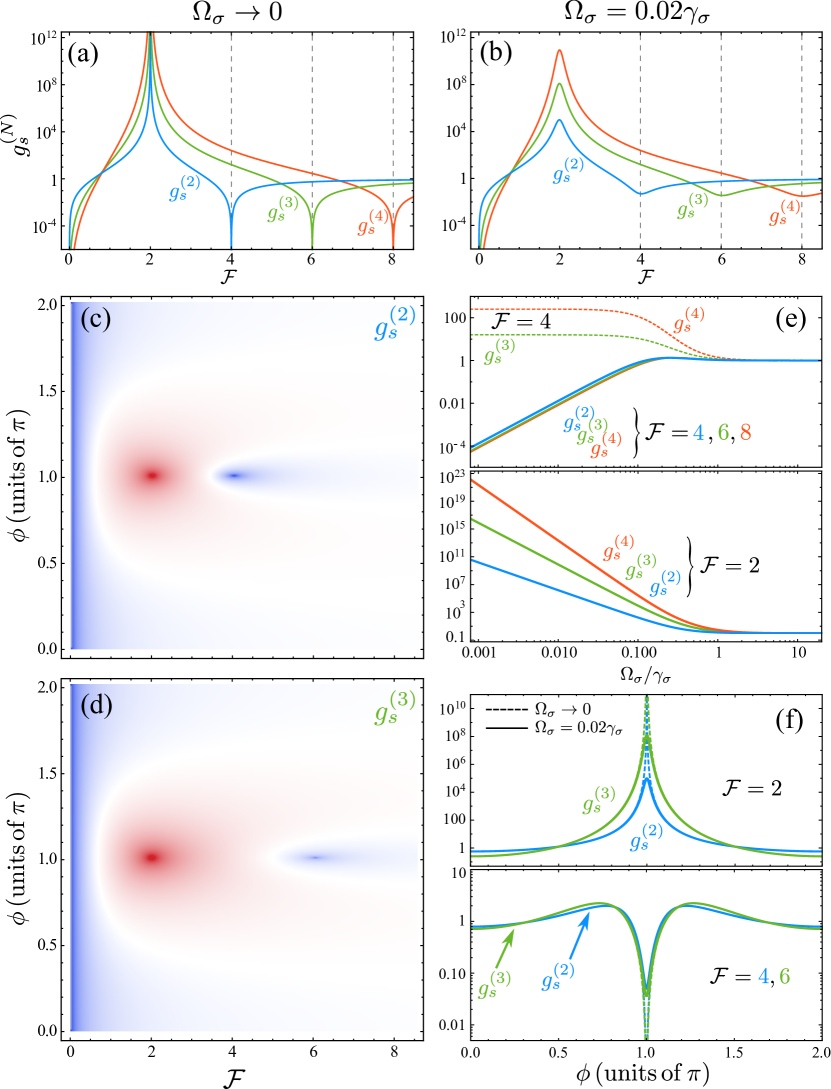
Figure 3: (Color online) $N$-photon statistics of a two-level system driven coherently at rate $\Omega_{\sigma}$ an homodyned (laser corrected) with a field of phase $\phi$ and amplitude a fraction $\mathcal{F}$ of $\Omega_{\sigma}$, in the limit of vanishing driving [(a), Eq. (41)] and for small but finite driving [(b), Eq. (42)]. (c), (d) Maps of two- and three-photon statistics as a function of the homodyning field. (e) Shows how correlations are weakened with increasing driving (solid lines) and how antibunching is realized at a given photon-number at a time, as opposed to bunching. Limits are given in Table 1. (f) shows the dependence on the phase of the homodyning field, for both vanishing and finite drivings for the case of bunching ($\mathcal{F}=2$) and two and three photon antibunching ($\mathcal{F}=4,6$). The only parameter has been taken as $\gamma_{\sigma}=1$.

	$\mathcal{F}=2$	4	6	8
$g^{(2)}_{s}$	$1/(64\Omega^{4})$	$128\Omega^{2}$
$g^{(3)}_{s}$	$1/(128\Omega^{6})$	16	$(729/8)\Omega^{2}$
$g^{(4)}_{s}$	$9/(4096\Omega^{8})$	256		$(524\,288/6561)\Omega^{2}$

Table 1: $N$-photon statistics with homodyning for the cases shown in Fig. 3(e), to leading-order in $\Omega$, in units of $\gamma_{\sigma}=1$.

Interestingly, suppressing the coherent contribution of the emission is not the only possibility. One can also tune the coherent contribution by choosing $\beta^{\prime}=e^{i\phi}|\beta^{\prime}|$, where the amplitude is parametrized as $|\beta^{\prime}|=\frac{\mathrm{R}}{\mathrm{T}}|\beta|$. The amplitude $|\beta^{\prime}|$ can be expressed more suitably in terms of the driving intensity of the laser: $|\beta^{\prime}|=\frac{\Omega_{\sigma}}{\gamma_{\sigma}}\mathcal{F}$. Thus, we are broadening the range of possible output configurations López Carreño et al. (2018), with $N$-particle correlators for the resonance-fluorescence plus an external laser having the following form, from which the population and two-photon statistics follow as special cases ($N=1,2$, respectively):

$$g^{(N)}_{s}=\frac{\mathrm{T}^{2N}}{\langle n_{s}\rangle^{N}}\frac{\mathcal{F}^{2(N-1)}\Omega_{\sigma}^{2N}}{\gamma_{\sigma}^{2N}\left(\gamma_{\sigma}^{2}+4\Delta_{\sigma}^{2}+8\Omega_{\sigma}^{2}\right)}\Big{[}4N^{2}\gamma_{\sigma}^{2}+{}\\ \mathcal{F}^{2}\left(\gamma_{\sigma}^{2}+4\Delta_{\sigma}^{2}+8\Omega_{\sigma}^{2}\right)+4N\mathcal{F}\gamma_{\sigma}\left(\gamma_{\sigma}\cos\phi-2\Delta_{\sigma}\sin\phi\right)\Big{]}$$ (41)

where $\langle n_{s}\rangle\equiv\langle{s^{\dagger}}s\rangle$, cf. Eq. (35b). These expressions are correct for any driving strength. However, in the Heitler regime, the results become ideal in the sense that antibunching becomes exactly zero and superbunching becomes infinite. In this case, Eq. (41) takes the simpler form:

$$g^{(N)}_{s}=\frac{|\beta^{\prime}|^{2(N-1)}\left(|\beta^{\prime}|^{2}+N^{2}\langle n_{\sigma}\rangle+2N\mathrm{Im}\{\alpha|\beta^{\prime}|e^{-i\phi}\}\right)}{\left(|\beta^{\prime}|^{2}+\langle n_{\sigma}\rangle+2\mathrm{Im}\{\alpha|\beta^{\prime}|e^{-i\phi}\}\right)^{N}}\,.$$ (42)

Both Eqs. (41) and (42) are shown in Fig. 3, where one can see how homodyning produces sharp resonances for various photon-numbers in antibunching and a common superbunching when the population vanishes. The case with no homodyning ($\mathcal{F}=0$) produces the best antibunching, both in magnitude (closest to zero), and in quality, namely, all $g^{(n)}$ go to zero simultaneously. This is antibuching in the sense tacitly understood for a single-photon source, separating photons the ones from the others, so it is apt to call it “conventional antibunching”, to differentiate it from the other type of two-photon antibunching, realized with an homodyning of $\mathcal{F}\neq 0$ and $\phi=0$. In the latter case, only $g^{(2)}$ is small and higher-order correlators are typically $\gg 1$. One can also, with different choice of $\mathcal{F}$, realize $n$-photon antibunching ($n=3$ and $4$ are shown in Fig. 3 in green and orange, respectively), but then again for a given photon number only. This follows from admixing a squeezed and coherent states as discussed in Section III and indeed the phenomenology of the homodyning of resonance fluorescence as shown in Fig. 3(b) is similar to that shown in Fig. 2(a) (with the coherent and squeezing fractions being tuned, respectively). In particular, and for the same reason, one also finds in resonance fluorescence the tunability of $g^{(n)}_{s}$ between zero to infinity, at small enough driving, simply by changing the coherent fraction. We call these features “unconventional.” Besides, this terminology fits (and has been chosen accordingly Zubizarreta Casalengua et al. (2020)) with the literature Ferretti et al. (2010); Flayac and Savona (2013); Majumdar and Gerace (2013); Gerace and Savona (2014); Flayac et al. (2015); Zhou et al. (2015); Tang et al. (2015); Cheng et al. (2017); Flayac and Savona (2017); Yu and Liu (2017); Wang et al. (2017); Snijders et al. (2018); Vaneph et al. (2018); Shen et al. (2018); Trivedi et al. (2019) which calls “unconventional” the supposed “blockade” that takes place when interfering fields Lemonde et al. (2014). They do not arise from a blockade from states of the system, as in the conventional scenario Birnbaum et al. (2005); Verger et al. (2006); Faraon et al. (2008, 2010); Hoffman et al. (2011); Rabl (2011); Lang et al. (2011); Müller et al. (2015); Radulaski et al. (2017); Deng et al. (2017); Sarma and Sarma (2017); Ghosh and Liew (2019); Delteil et al. (2019), but from an interference. Note that unconventional superbunching, unlike unconventional antibunching, is simultaneously bunched at all photon-orders. Actually, this also follows from the cancellation of a correlator, namely, the first-order one (population) with the result of having all higher-order correlators diverging. For non-vanishing driving, the features are qualitatively similar but strongly damped, as shown on the right column of Fig. 3. Panel (e) gives a quantitative account of how correlations weaken with driving. The trend of antibunching/superbunching with $\Omega$ is easily obtained from a series expansion of Eq. (41) and is given in Table 1 to leading order in $\Omega$ (to next order, for instance, $g^{(2)}_{s}(\mathcal{F}=2)=1/(64\Omega^{4})+1/(4\Omega^{2})$ and $g^{(3)}_{s}(\mathcal{F}=4)=16-768\Omega^{2}$). This also shows for the case of two-photon antibunching how only $g^{(2)}_{s}$ improves while higher-orders (dashed) saturate. As shown in panel (c) and (d), in this case, the phase of the homodyning is the same (for the anharmonic oscillator, for instance, it is $N$-dependent Zubizarreta Casalengua et al. (2020))). The sensitivity of the effect to the phase and driving strength is shown quantitatively in panel (f).

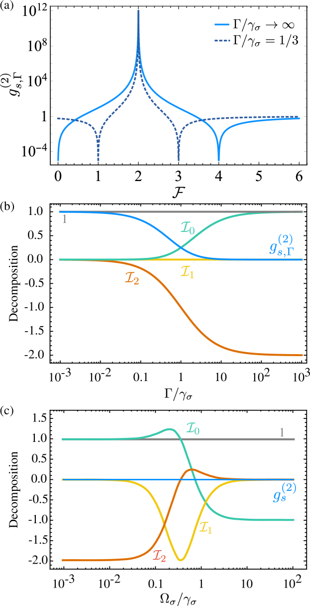
Figure 4: (Color online) (a) Two-photon statistics of a two-level system in the Heitler limit with (dashed-dark) and without (solid-light blue) filtering as a function of the homodyning amplitude $\mathcal{F}$. Conventional antibunching gets spoiled by filtering but perfect unconventional antibunching is obtained with homodyning. (b) Evolution of the $\mathcal{I}$ parameters as a function of the filter’s width $\Gamma$ showing how filtering disrupts the perfect cancellation of $g^{(2)}_{s,\Gamma}$. Homodyning restores the condition $\mathcal{I}_{2}=-2\mathcal{I}_{0}$. (c) Evolution of the $\mathcal{I}$ parameters as a function of pumping strength $\Omega_{\sigma}$. Without filtering, the cancellation is still perfect at all pumpings but involves $\mathcal{I}_{1}$ and thus cannot be fully restored with homodyning.

One could naturally question why going to the extent of homodyning since the case $\mathcal{F}=0$ may appear superior in several respects, in particular, at non-vanishing pumping. Beyond the fact that conventional and unconventional statistics stem from two different types of light, which may have some interest per se, one obvious application is to restore antibunching which has been lost as a result of filtering. It is now amply demonstrated that frequency filtering spoils antibunching of resonance fluorescence Phillips et al. (2020); Hanschke et al. (2020). The reason for this in the Heitler regime is shown in Fig. 4, that displays in Panel (b) the $\mathcal{I}$ coefficients in the Heitler regime in presence of filtering $\Gamma$ (this can also be obtained from the wavefunction approximation method Visser and Nienhuis (1995) as detailed in the Supplementary Material for this and other systems studied in this text):

$$\mathcal{I}_{0} ={\Gamma^{2}\over(\Gamma+\gamma_{\sigma})^{2}}\,,$$ (43a)

$$\mathcal{I}_{1} =0\,,$$ (43b)

$$\mathcal{I}_{2} =-{2\Gamma\over\Gamma+\gamma_{\sigma}}$$ (43c)

which shows how the filter perturbs the balance of the $\mathcal{I}$ coefficients, with $\mathcal{I}_{2}$ going to zero faster than $\mathcal{I}_{0}$, resulting in the sum taking off as

$$g_{s,\Gamma}^{(2)}=\left({\gamma_{\sigma}\over\Gamma+\gamma_{\sigma}}\right)^{2}\,.$$ (44)

While the conventional antibunching is irretrievably lost, unconventional two-photon antibunching now gets two conditions to be restored, at $\mathcal{F}=2(1\pm\sqrt{\Gamma/(\Gamma+\gamma_{\sigma}})$ López Carreño et al. (2018). The case $\Gamma/\gamma_{\sigma}=1/3$ is shown in Fig. 4(a). At this sub-natural linewidth filtering, conventional antibunching has reduced from exactly zero in the Heitler limit to $9/16\approx 0.56$, but perfect antibunching can be restored with $\mathcal{F}=2\pm 1$. Both resonances are unconventional in the sense that successive higher-order correlators have non-matching resonances López Carreño et al. (2019), but in both cases, perfect antibunching can be restored, regardless of the filter’s width, by bringing back $\mathcal{I}_{0}$ and $\mathcal{I}_{2}$ to 2 and 1, respectively, with the appropriate correction of the coherent fraction.

Restoring such a perfect cancellation of the $\mathcal{I}$ coefficients works exactly in the Heitler limit and at vanishing driving. At non-vanishing driving, the $\mathcal{I}$ parameters (11) read

$$\mathcal{I}_{0} =\frac{|\alpha|^{2}\left(6\langle n_{\sigma}\rangle-4|\alpha|^{2}\right)}{n_{\sigma}^{2}}-1\,,$$ (45a)

$$\mathcal{I}_{1} =-8\frac{|\alpha|^{2}\left(\langle n_{\sigma}\rangle-|\alpha|^{2}\right)}{n_{\sigma}^{2}}\,,$$ (45b)

$$\mathcal{I}_{2} =2\frac{|\alpha|^{2}\left(\langle n_{\sigma}\rangle-2|\alpha|^{2}\right)}{n_{\sigma}^{2}}\,.$$ (45c)

In this case, as seen in Fig. 4(c), perfect antibunching does not follow simply from $\mathcal{I}_{2}=-2\mathcal{I}_{0}$ but also involves $\mathcal{I}_{1}$ which is related to anomalous quadrature moments, that a displaced-thermal squeezed state does not possess, therefore causing a breakdown of the Gaussian-states approximation. Since it also depends on $\alpha$, it becomes impossible to realize another perfect cancellation, or restore it if spoiled, since the sum depends in multiple ways on the one free parameter: the homodyning signal. As a result, the minimum antibunching is now finite, as shown in Fig. 3(b). At still higher pumping, $\Omega_{\sigma}\gg\gamma_{\sigma}$, in the so-called Mollow regime, antibunching comes exclusively from $\mathcal{I}_{0}$, which is the antibunching of an incoherently-pumped two-level system with non-Gaussian fluctuations. In this limit, $\langle d^{\dagger}d\rangle=\langle n_{s}\rangle$, which absorbs the term 1 in Eqs. (7). There is no way to correct for the coherent component in this case since there is no coherence involved.

We conclude this section by using the self-homodyning approach to further characterize the nature of the admixing, which we now show, corresponds to lowest order in the driving to a coherent state for $\langle\sigma\rangle$, which is a tautology, and to a squeezed thermal state for the fluctuations $\mathcal{\epsilon}$. Two quantities allow to identify squeezing in a quantum field $\epsilon$, namely, the mean $\langle X_{\epsilon,\chi}\rangle$ of the quadratures $X_{\epsilon,\chi}\equiv\frac{1}{2}(e^{i\chi}{\epsilon^{\dagger}}+\mathrm{c.c.})$ for the operator $\epsilon$ with phase $\chi$, as well as the variance (dispersion) $\langle\Delta X_{\epsilon,\chi}^{2}\rangle=\langle X_{\epsilon,\chi}^{2}-\langle X_{\epsilon,\chi}\rangle^{2}\rangle$. Note that this could also be done directly for the full field $\sigma$ since this only adds the comparatively trivial contribution of the coherent state $\langle\sigma\rangle=\alpha$. The maximum and minimum of the normal-ordered quadrature variance for a single-mode can be computed independently of the specific nature of the field:

$$\langle:\Delta X_{\epsilon}^{2}:\rangle_{\mathrm{max}/\mathrm{min}}=\langle\Delta X_{\epsilon}^{2}\rangle_{\mathrm{max}/\mathrm{min}}-\frac{1}{4}\\ {}=\frac{1}{2}\left[\pm|\langle\epsilon^{2}\rangle-\langle\epsilon\rangle^{2}|+\langle{\epsilon^{\dagger}}\epsilon\rangle-|\langle\epsilon\rangle|^{2}\right]\,,$$ (46)

where the sign corresponds to the maximum and minimum, respectively. While the variance is positive, its normal-ordered counterpart does not have to be. The deviation of the variance from the vacuum value (which is $\frac{1}{4}$) to negative values reveals some degree of quadrature squeezing. Likewise, the angle of squeezing is generically given by $\theta=\mathrm{arg}\left[\langle\epsilon^{2}\rangle-\langle\epsilon\rangle^{2}\right]$. One gets, by substituting the correlators (36) in (46),

$$\langle:\Delta X_{\epsilon}^{2}:\rangle_{\mathrm{min}}=-\frac{2\Omega_{\sigma}^{2}\left(\gamma_{\sigma}^{2}+4\Delta_{\sigma}^{2}-8\Omega_{\sigma}^{2}\right)}{\left(\gamma_{\sigma}^{2}+4\Delta_{\sigma}^{2}+8\Omega_{\sigma}^{2}\right)^{2}},$$ (47a)

$$\langle:\Delta X_{\epsilon}^{2}:\rangle_{\mathrm{max}}=\frac{2\Omega_{\sigma}^{2}}{\gamma_{\sigma}^{2}+4\Delta_{\sigma}^{2}+8\Omega_{\sigma}^{2}},$$ (47b)

with the angle of squeezing $\theta=\mathrm{arg}[(\gamma_{\sigma}-2i\Delta_{\sigma})^{2}]$. Analyzing the sign of these quantities would therefore allow us to infer squeezing. This is made particularly clear in the low-driving regime ($\Omega_{\sigma}\rightarrow 0$), where the previous expressions at the lowest order in $\Omega_{\sigma}$ simplify to

$$\langle:\Delta X^{2}_{\epsilon}:\rangle_{\mathrm{max}/\mathrm{min}}\approx\pm\frac{2\Omega_{\sigma}^{2}}{\gamma_{\sigma}^{2}+4\Delta^{2}_{\sigma}}\,.$$ (48)

In this limit, the two extrema of the normal-ordered variance are simply symmetrical around zero, so $\langle:\Delta X^{2}_{\epsilon}:\rangle$ is always negative and fluctuations thus always bear some indication of squeezing. We can furthermore recognize these expressions as a limit of low squeezing from a displaced squeezed thermal state. When $r\rightarrow 0$, such states have the variance

$$\langle:\Delta X^{2}:\rangle_{\mathrm{max}/\mathrm{min}}^{\mathrm{DST}}\approx\frac{1}{4}\left[\left(1\pm 2r\right)\left(1+2\langle n_{\mathrm{th}}\rangle\right)-1\right]\approx\pm\,\frac{r}{2},$$ (49)

where the superscript DST means that the observable corresponds to an exact displaced squeezed thermal state. We have approximated $1+2\langle n_{\mathrm{th}}\rangle$ to $1$ since the thermal population grows like $\Omega_{\sigma}^{4}$ (which comes from the first-order of the incoherent population). Comparing Eq. (48) with Eq. (49) shows that the incoherent population in the Heitler regime behaves like a squeezed thermal state with effective squeezing parameter $r_{\mathrm{eff}}$ and effective thermal population $\mathrm{p}_{\mathrm{th}}$

$$r_{\mathrm{eff}}=\frac{4\Omega_{\sigma}^{2}}{\gamma_{\sigma}^{2}+4\Delta_{\sigma}^{2}}\quad{\text{and}}\quad\mathrm{p}_{\mathrm{th}}\approx\frac{16\Omega_{\sigma}^{4}}{\left(\gamma_{\sigma}^{2}+4\Delta_{\sigma}^{2}\right)^{2}}\,.$$ (50)

From these two parameters, an effective $g^{(2)}$, namely $g^{(2)}_{\mathrm{eff}}$, can be obtained for the fluctuations. Supposing that, in the low-excitation regime, the state of fluctuations is that of a squeezed thermal state, then $g^{(2)}_{\epsilon}$ should have the same form. Fixing $|\alpha|=0$ in Eq. (20b) and taking the limit $r^{2}\rightarrow 0$ and $\mathrm{p}_{\mathrm{th}}\rightarrow 0$ (both go to 0 with the same power dependence), we get

$$g^{(2)}_{\mathrm{eff}}\approx\frac{r_{\mathrm{eff}}^{2}}{\left(r_{\mathrm{eff}}^{2}+\mathrm{p}_{\mathrm{th}}\right)^{2}},$$ (51)

which, after substituting Eqs. (50), reads as

$$g^{(2)}_{\mathrm{eff}}\approx\frac{\left(\gamma_{\sigma}^{2}+4\Delta_{\sigma}^{2}\right)^{2}}{64\Omega_{\sigma}^{4}}\,.$$ (52)

This simple expression is a good approximation to the exact result Eq. (40) that gives the statistics of the fluctuations. As was the case when admixing a pure coherent-state to a coherent state in Section III, antibunching of the total signal $g_{s}^{(2)}<1$ is obtained from a coherent state and a superbunched $g^{(2)}_{\epsilon}\gg 1$ (even diverging $g^{(2)}_{\mathrm{eff}}\rightarrow\infty$) squeezed state.

VI Jaynes–Cummings statistics

The same analysis as above can be transported to a wealth of other systems. For instance, in the case of an anharmonic oscillator, new resonances appear and with richer phase conditions than those of a two-level system Zubizarreta Casalengua et al. (2020). We go directly to a fundamental and natural system where to apply the concepts above, namely, the Jaynes–Cummings model Jaynes and Cummings (1963); Shore and Knight (1993), since this adds to the two-level system a quantized optical mode (a cavity) with a total emission that, therefore, consists intrinsically of the mixing of a quantum (two-level system) and a coherent (cavity) signals. The photon statistics of this system has been for decades observed in one way or another to exhibit resonances which are a simple and direct manifestation of self-homodyning in the wake of the previous sections, but which have often been merely taken as the brute result of numerical simulations. We now provide what we believe is the appropriate physical picture to unify, classify, and understand such results. Given the role of the amplitude and phase of the fields in phenomena that are ultimately interferences, we include in the Hamiltonian two driving terms, one for the emitter, $\Omega_{\sigma}$, the other for the cavity $\Omega_{a}$. Their relative phase $\phi$ and the ratio of their amplitude $\chi\equiv\Omega_{\sigma}/\Omega_{a}$ will play a role in tuning the statistics. The Hamiltonian therefore reads as

$$H_{\mathrm{jc}}=\Delta_{\sigma}{\sigma^{\dagger}}\sigma+\Delta_{a}{a^{\dagger}}a+g\left({a^{\dagger}}\sigma+{\sigma^{\dagger}}a\right)+{}\\ {}+\Omega_{a}\left(e^{i\phi}{a^{\dagger}}+e^{-i\phi}a\right)+\Omega_{\sigma}\left({\sigma^{\dagger}}+\sigma\right).$$ (53)

Solving for the steady state in the low-driving regime, i.e., when $\Omega_{a,\sigma}\ll\gamma_{a}\,,\gamma_{\sigma}$, yields for the populations:

$$\langle n_{\begin{subarray}{c}a\\ \sigma\end{subarray}}\rangle=4\,\frac{4g^{2}\Omega_{\begin{subarray}{c}a\\ \sigma\end{subarray}}^{2}+\Gamma_{\begin{subarray}{c}\sigma\\ a\end{subarray}}^{2}\Omega_{\begin{subarray}{c}a\\ \sigma\end{subarray}}^{2}-4g\Omega_{a}\Omega_{\sigma}\left(\pm 2\Delta_{\begin{subarray}{c}a\\ \sigma\end{subarray}}\cos\phi+\gamma_{\begin{subarray}{c}\sigma\\ a\end{subarray}}\sin\phi\right)}{16g^{4}+8g^{2}\left(\gamma_{a}\gamma_{\sigma}-4\Delta_{a}\Delta_{\sigma}\right)+\Gamma_{a}^{2}\Gamma_{\sigma}^{2}}\,,$$ (54)

with matching upper/lower indices (including $\pm$) and with $\Gamma^{2}_{i}=\gamma_{i}^{2}+4\Delta_{i}^{2}$ (for $i=a,\sigma$). Similarly, the two-photon coherence function from the cavity can be found as:

$$\begin{split}g^{(2)}_{a}=&\Big{\{}\Big{[}16g^{4}+8g^{2}\left(\gamma_{a}\gamma_{\sigma}-4\Delta_{a}\Delta_{\sigma}\right)+\Gamma_{a}^{2}\Gamma^{2}_{\sigma}\Big{]}\Big{[}16g^{4}\left(1+\chi^{4}\right)+8g^{2}\big{(}2\chi^{2}\Gamma_{11}^{2}+4\Delta_{\sigma}\tilde{\Delta}_{11}-\gamma_{\sigma}\tilde{\gamma}_{11}\big{)}+\Gamma^{2}_{\sigma}\Gamma_{11}^{2}-\\ &16g\chi\big{(}\Delta_{\sigma}\Gamma_{11}^{2}+4g^{2}\tilde{\Delta}_{11}[1+\chi^{2}]\big{)}\cos\phi+8g^{2}\chi^{2}\big{(}4g^{2}-\gamma_{\sigma}\tilde{\gamma}_{11}+4\Delta_{\sigma}\tilde{\Delta}_{11}\big{)}\cos 2\phi\,-\\ &8g\chi\big{(}\gamma_{\sigma}\Gamma_{11}^{2}+4g^{2}\tilde{\gamma}_{11}[\chi^{2}-1]\big{)}\sin\phi+16g^{2}\chi^{2}\big{(}\gamma_{a}\Delta_{\sigma}+\gamma_{\sigma}\tilde{\Delta}_{12}\big{)}\sin 2\phi\Big{]}\Big{\}}\Big{/}\\ &\Big{\{}\Big{[}16g^{4}+8g^{2}\Big{(}\gamma_{a}\tilde{\gamma}_{11}-4\Delta_{a}\tilde{\Delta}_{11}\Big{)}+\Gamma_{a}^{2}\Gamma_{11}^{2}\Big{]}\Big{[}4g^{2}\chi^{2}+\Gamma_{\sigma}^{2}-4g\chi\big{(}2\Delta_{\sigma}\cos\phi+\gamma_{\sigma}\sin\phi\big{)}\Big{]}^{2}\Big{\}},\end{split}$$ (55)

where $\tilde{\Delta}_{ij}\equiv i\Delta_{a}+j\Delta_{\sigma}$, $\tilde{\gamma}_{ij}=i\gamma_{a}+j\gamma_{\sigma}$ and $\Gamma_{ij}^{2}\equiv\tilde{\gamma}_{ij}^{2}+4\tilde{\Delta}^{2}_{ij}$. The range of $\chi$ extends from 0 to $\infty$ so that it is convenient to use the derived quantity $\tilde{\chi}=\frac{2}{\pi}\atan(\chi)$ which varies between 0 and 1. The expressions above are cumbersome but they are covering a considerable amount of phenomenology, each variation of which could give rise to an independent numerical study of its own. Let us start with the much simpler-looking particular case of one pumping only, namely, with cavity-pumping only, which is the case most discussed in the literature. Then Eq. (55) reduces to:

$$g^{(2)}_{a}=[16g^{4}+8g^{2}\left(\gamma_{\sigma}\gamma_{a}-4\Delta_{a}\Delta_{\sigma}\right)+\Gamma_{a}^{2}\Gamma_{\sigma}^{2}][16g^{4}-8g^{2}(\gamma_{\sigma}\tilde{\gamma}_{11}-4\Delta_{\sigma}\tilde{\Delta}_{11})+\Gamma_{\sigma}^{2}\tilde{\Gamma}_{11}^{2}]\big{/}\Gamma_{\sigma}^{4}[16g^{4}+8g^{2}(\gamma_{a}\tilde{\gamma}_{11}-4\Delta_{a}\tilde{\Delta}_{11})+\Gamma_{a}^{2}\tilde{\Gamma}_{11}^{2}]\,.$$ (56)

A density plot of Eq. (56) is shown in Fig. 5(a) where one sees that the formula produces simple features in the form of well-defined lines of antibunching (blue in our color code) and bunching (red), as a function of the relevant parameters (pumping, lifetimes, etc.) The general expression, Eq. (55) is shown in the facing panel 5(b) for the case of a balanced driving $\Omega_{a}=\Omega_{\sigma}$ ($\tilde{\chi}=0.5$) with also a relative phase of $\pi/2$ between the two drivings. Other cases can be visualised interactively with an applet Zubizarreta Casalengua et al. (2018). Depending on the configuration, one sees that some features appear while other disappear, e.g., the horizontal superbunched line disappears and a diagonal antibunched line appears, with also two antibunched hyperbolas now absent. We remind that the change from one case to the other comes merely from switching on a second and out-of-phase driving term from $\Omega_{\sigma}=0$ (left) to $\Omega_{\sigma}=\Omega_{a}$ (right). One can see how, as a result, in the configuration of driving the system and detecting the photons both at resonance ($\omega_{\mathrm{L}}=\omega_{A}=0$), there is a drastic change from giant superbunching ($g^{(2)}=1.6\times 10^{9}$) when driving the cavity, to strong antibunching ($g^{(2)}=0.01$) when also driving the emitter. This is an illustration of how greatly tunable is the photon statistics, this times through the balance of the coherent fields involved.

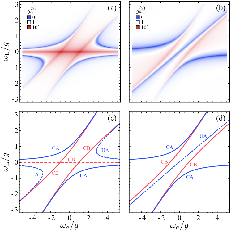
Figure 5: (Color online) Landscape of two-photon correlations in the Jaynes–Cummings system, for cavity driving only (left, with $\tilde{\chi}=0$) and mixed driving (right, with $\tilde{\chi}=0.5$ and $\phi=\pi/2$), as a function of where the system is driven ($\omega_{\mathrm{L}}$) and where it is emitting ($\omega_{a}$). The top row shows the exact results, Eq. (55) left and Eq. (56) right, and the bottom row its classification in terms of Conventional (C) and Unconventional (U) features of Antibunching (A) and Bunching (B), namely, Eq. (57) with $N=1$ for CA (solid blue) and $N=2$ for CB (solid red), and Eq. (60) for UA (dashed blue). For the left case with cavity-pumping only, the UA simplifies to Eq. (62). Parameters: $g=1$, $\gamma_{a}=0.1$ and $\gamma_{\sigma}=0.01$.

We now address the qualitative meaning of each line. Some of the features, shown in Fig. 5, are easily recognized, namely, the lower and upper polaritons, with their characteristic anticrossing, and even more simply, the bare states of the cavity (horizontal line) and two-level system (diagonal). Their expressions are consequently easily found, as $\omega_{a}$, $\omega_{\sigma}$ for the bare states and del Valle et al. (2009); Laussy et al. (2012)

$$E^{(N)}_{\pm}=N\omega_{a}+\frac{\omega_{\sigma}-\omega_{a}}{2}\\ \pm\mathrm{Re}\sqrt{(\sqrt{N}g)^{2}+\left(\frac{\omega_{a}-\omega_{\sigma}}{2}-i\frac{\gamma_{a}-\gamma_{\sigma}}{4}\right)^{2}}\,,$$ (57)

with $N=1$ for the single polaritons and $N=2$ for the two-excitation polaritons. Equation (57) with $N=1$ yields the blue solid lines labelled CA, for “conventional antibunching”, in Fig. 5(c–d). At the $g^{(2)}$ level, only features up to $N=2$ show up, but if one considers higher-order photon correlations, then higher rungs of the Jaynes–Cummings ladder are probed and the traces formed by Eq. (57) for $N\leq k$ are seen in $g^{(k)}$, as is shown in Fig. 6 for $N$ up to $4$. Although these features can appear only at a given photon-number $N$, their position is otherwise fixed.

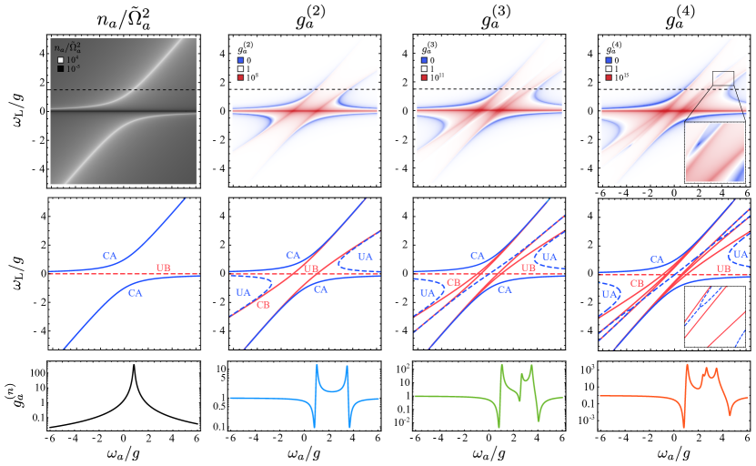
Figure 6: (Color online) Conventional and unconventional features at the $N=1,2,3$ and $4$-photon level. Upper row shows the numerically exact landscapes of $N$-photon observables, from the population normalized to the relative laser intensity $\tilde{\Omega}_{a}^{2}=\Omega_{a}^{2}/\gamma_{a}^{2}$ ($N=1$, left) till four-photon correlations ($N=4$ right). Middle-row shows the theoretical lines that reproduce these structures and their classifications as conventional (C, solid) and unconventional (U, dashed) bunching (red) and antibunching (blue), respectively. Bottom row shows the cuts along the horizontal dashed line in the top row. The inset in $g^{(4)}_{a}$ magnifies a forking of antibunching. Parameters are the same as in Fig. 5(a).

We note also that although we consider throughout strong-coupling configurations, and its underlying dressed-states structure, there is not such a clear-cut distinction between strong and weak-coupling, as discussed in more details in Ref. Zubizarreta Casalengua et al. (2020), where a critical coupling strength $g_{P}$ between the cavity and the 2LS that results in Poissonian statistics ($g^{(2)}_{a}=1$), is compared to bunching/antibunching in the system. We do not discuss this further but give its closed-form expression:

$$g_{P}=\frac{1}{2}\Big{\{}\big{[}16\Delta_{\sigma}^{4}+32\Delta_{a}\Delta_{\sigma}^{3}-8(\gamma_{a}^{2}+3\gamma_{a}\gamma_{\sigma}+\gamma_{\sigma}^{2}-4\Delta_{a}^{2})\Delta_{\sigma}^{2}\\ {}-8\gamma_{\sigma}(4\gamma_{a}+3\gamma_{\sigma})\Delta_{a}\Delta_{\sigma}+\gamma_{\sigma}^{2}(2\gamma_{a}^{2}+2\gamma_{a}\gamma_{\sigma}+\gamma_{\sigma}^{2}-8\Delta_{a}^{2})\big{]}^{1/2}+{}\\ \gamma_{\sigma}^{2}-4\Delta_{\sigma}^{2}\Big{\}}^{1/2}.$$ (58)

A smaller coupling $g<g_{\mathrm{P}}$ produces antibunched light while a larger coupling $g>g_{\mathrm{P}}$ produces bunched light.

Less immediate to identify are the other features, not accounted for by Eq. (57), but that can be extracted from Eq. (55). This can be conveniently done since the features already identified do not provide the best antibunching, which is produced by the unconventional mechanism instead and we have seen that this reaches exactly zero in the vanishing driving limit. One can thus hope to find the condition for the other lines simply by solving $g^{(2)}_{a}=0$ with $\Omega_{a,\sigma}\rightarrow 0$, which yields the following condition (see also the Supplemental Material):

$$\Delta_{a}=\Big{[}i\big{(}\gamma_{\sigma}+2i\Delta_{\sigma}\big{)}\big{(}\tilde{\gamma}_{11}+2i\Delta_{\sigma}\big{)}+{}\\ {{}+4e^{-i\phi}g\,\chi\big{(}\tilde{\gamma}_{11}+2i\Delta_{\sigma}\big{)}-4ig^{2}\big{(}1+e^{-2i\phi}\chi^{2}\big{)}}\Big{]}\bigg{/}\\ ({2\gamma_{\sigma}+4i\Delta_{\sigma}-8ie^{-i\phi}g\,\chi})\,.$$ (59)

The expression is, in general, complex, which means that one fails to get exactly $g^{(2)}_{a}=0$. Given that we are now dealing with self-homodyning, there is no guarantee indeed that the system would interfere its coherent and quantum component so as to cancel exactly a given photon-number statistics. Instead, there is the need for a fine tuning, which, if not enforced externally as was the case in the previous Sections, can only be realized fortuitously. This account for the sharpness of the resonances as the exact conditions to produce a perfect cancellation requires a careful balancing which is realized at an isolated point of the configuration space. Taking the real part, however, happens to provide the condition for Unconventional Antibunching (UA) that accounts for the features not produced by Eq. (57). The expression then reads as

$$\Delta_{a}=\frac{4g\chi\big{\{}2\cos\phi\big{[}2\Delta_{\sigma}^{2}+g^{2}\big{(}1+\chi^{2}\big{)}\big{]}-g\chi\Delta_{\sigma}\cos 2\phi-\gamma_{\sigma}\sin\phi\big{(}g\chi\cos\phi-2\Delta_{\sigma}\big{)}\big{\}}-\Delta_{\sigma}\big{[}\Gamma^{2}_{\sigma}+4g^{2}\big{(}1+4\chi^{2}\big{)}\big{]}}{\gamma_{\sigma}^{2}+4\big{(}\Delta_{\sigma}^{2}+4g^{2}\chi^{2}\big{)}-8g\chi\big{(}2\Delta_{\sigma}\cos\phi+\gamma_{\sigma}\sin\phi\big{)}}\,.$$ (60)

Equation (60) yields the blue dashed lines labelled UA in Fig. 5(c–d). All CA, UA, CB and UB lines are easily recognized in the numerically exact plots in Panels (a–b), which fit perfectly with the theoretical lines for small enough $\Omega_{a,\sigma}$. Further imposing the imaginary part to be also zero finds the isolated points where $g^{(2)}_{a}=0$ exactly, which provides a second expression:

$$\Delta_{\sigma}=\frac{4g\chi\cos\phi\,(\tilde{\gamma}_{11}-g\chi\sin\phi)\pm\sqrt{-\tilde{\gamma}_{11}(\gamma_{\sigma}-4g\chi\sin\phi)[-4g^{2}+\gamma_{\sigma}\tilde{\gamma}_{11}-4g\chi(g\chi\cos 2\phi+\tilde{\gamma}_{11}\sin\phi)]+4g^{2}\chi^{2}\sin^{2}2\phi}}{2\tilde{\gamma}_{11}}\,.$$ (61)

Since Eq. (61) has to be real, the radicand has to be positive. For the particular case $\chi=0$, which is that of main interest, these expressions simplify considerably, namely, Eq. (60) becomes

$$\Delta_{a}=-\Delta_{\sigma}\left(1+\frac{4g^{2}}{\gamma_{\sigma}^{2}+4\Delta_{\sigma}^{2}}\right)\,,$$ (62)

and Eq. (61) becomes

$$\Delta_{\sigma}=\pm\sqrt{\frac{\gamma_{\sigma}g^{2}}{\tilde{\gamma}_{11}}-\frac{\gamma_{\sigma}^{2}}{4}}\,.$$ (63)

These conditions give, first, the UA dashed lines shown, in Fig. 5(c) and, second, the optimum points along these curves. Thus, with mixed driving (Eqs. (60–61)) or cavity-only driving (Eqs. (62–63)), both conditions taken together provide where to drive and detect the Jaynes–Cummings system to reach perfect $g^{(2)}_{a}$ cancellation.

The complexity of photon correlations when including all orders can hardly be exaggerated. Figure 6 shows how the configuration of Fig. 5(a) appears when resolved to different photon numbers ($1\leq N\leq 4$). At the single-photon level, left column, which is simply luminescence, or any measurement of the population $n_{a}$ of the system, one only resolves the familiar anticrossing of the two dressed states, or polaritons. A cut as shown in the bottom-left panel is simply a Lorentzian function whose width is given by the effective lifetime of the system $\gamma_{U}=\big{(}\gamma_{a}+\frac{4g^{2}\gamma_{\sigma}}{\Gamma_{\sigma}^{2}}\big{)}/2$. There is actually one feature which is not typically considered given its intrinsically impractical measurement, namely, the horizontal black line at $\omega_{\mathrm{L}}=0$ which exhibits a suppression of the population. There is much less light emitted there than at any random point. This anomalously faint light, however, comes with very strong correlations, to all-orders, as is revealed in the other panels where this line shows up as unconventional bunching. This results precisely from the self-homodyning of the system cancelling largely the coherent contribution of the emission, leaving mainly quantum fluctutations, or, here one could say, quantum noise, that has superbunched statistics.

At the two-photon level, on the second column of Fig. 6, one finds again the polariton lines, which are antibunched, according to the conventional blockade scenario, whence the label CA. They are supplemented by two unconventional, self-homodyning antibunching lines UA, in dashes, as well as the $N=2$ polariton dressed states of Eq. (57) which, by two-photon absorption, now exhibit conventional bunching CB. There is a beautiful symmetry and even proximity of these resonances, although they can be of a different character (antibunching and bunching) and origin (conventional and unconventional). Note, in particular, in the bottom panel how the CA and UA exhibit an essentially identical value. At the three-photon level, on the third column, and even more so at the four-photon level, fourth column, one now finds a proliferation of CB features, due to involving the higher rungs of the Jaynes-Cummings ladder, although these simply add to the lines already existing. In contrast, as already commented, the UA lines shift positions. There also appears more UA lines, as can be seen in $g^{(3)}_{a}$ with the appearance of a diagonal UA line, that further exhibits a fork at the four-photon level. One can check that this complicated structure, predicted by the theory, is reproduced and easily identified in the numerically exact landscape of correlation, as shown in the inset of $g^{(4)}_{a}$ where the branch crossing of antibunching is clearly resolvable, despite being surrounded by conventional bunching lines. The cuts in the bottom row consequently exhibit extremely complex resonances alternating between giant bunching and antibunching, whose relative interplay account for the relative values found in each case.

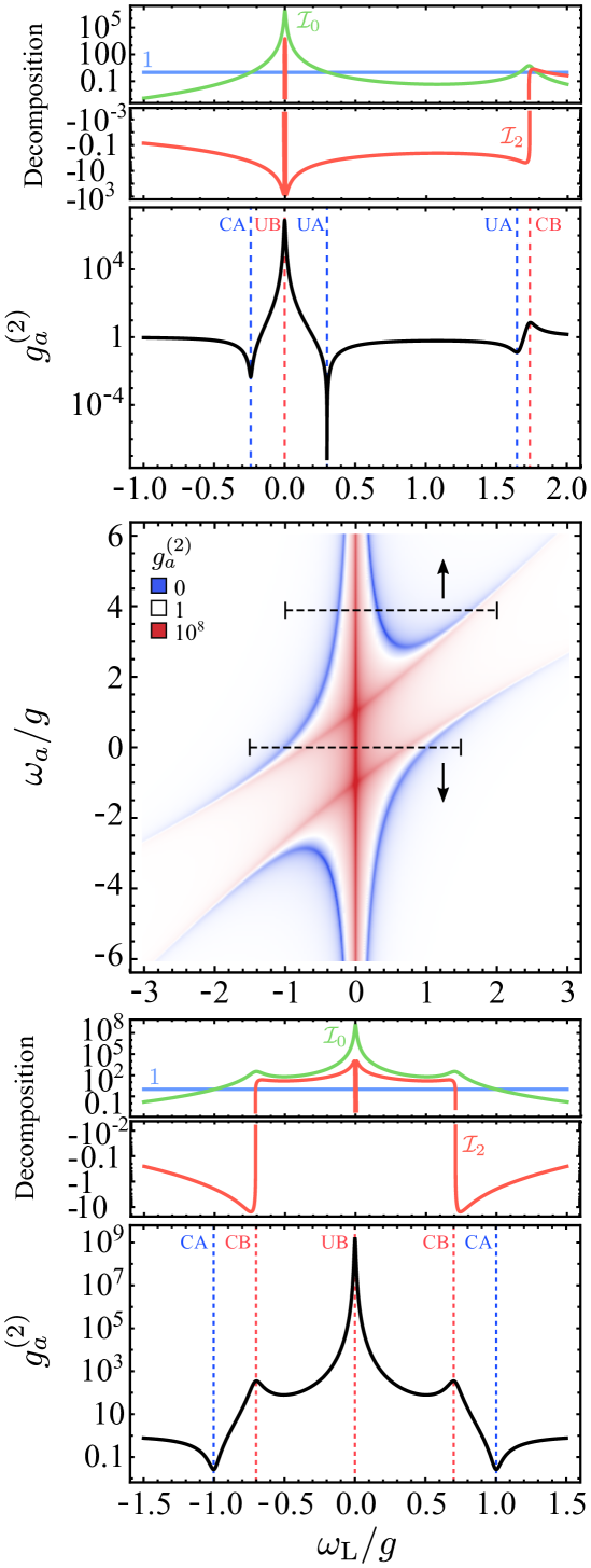
Figure 7: (Color online) Decomposition of the Jaynes–Cummings statistics into its $\mathcal{I}$ coefficients (in log-scales, separating the positive and negative components) for the two cuts shown in the middle panel. The upper case captures one of the exactly-zero antibunching, on the UA line. Parameters are the same as in Fig. 5(a).

This complex phenomenology fits with the simple classification above and can also be simply understood as multiphoton interferences, as can be illustrated by their decomposition in terms of the $\mathcal{I}$ parameters of Eq. (7) (the same could be done for the $\mathcal{J}$, $\mathcal{K}$ parameters, etc.) In this dynamical case, the decomposition (11) yields the following expressions, when the cavity alone is driven ($\chi=0$) at vanishing pumping (although the general case could also be provided, there is no need to for the present discussion):

$$\mathcal{I}_{0}= \ 256g^{8}\bigm{/}f_{1}\left(g,\Delta_{a,\sigma},\gamma_{a,\sigma}\right)\,,$$ (64a)

$$\mathcal{I}_{1}= \ 0\,,$$ (64b)

$$\begin{split}\mathcal{I}_{2}=&\ 32g^{4}\bigg{[}-\gamma_{\sigma}^{2}\Big{(}4g^{2}+\gamma_{a}\left(\gamma_{a}+\gamma_{\sigma}\right)-4\Delta_{a}^{2}\Big{)}\\ &{}+4\gamma_{\sigma}\left(4\gamma_{a}+3\gamma_{\sigma}\right)\Delta_{a}\Delta_{\sigma}-16\Delta_{a}\Delta_{\sigma}^{3}+{}\\ 4\Delta_{\sigma}^{2}&\Big{(}4g^{2}+\gamma_{a}\left(\gamma_{a}+\gamma_{\sigma}\right)-4\Delta_{a}^{2}\Big{)}\bigg{]}\biggm{/}f_{1}\left(g,\Delta_{a,\sigma},\gamma_{a,\sigma}\right)\,,\end{split}$$ (64c)

where the function $f_{1}\left(g,\Delta_{a,\sigma},\gamma_{a,\sigma}\right)$ is defined as:

$$f_{1}\left(g,\Delta_{a,\sigma},\gamma_{a,\sigma}\right)=\Big{(}\gamma_{\sigma}^{2}+4\Delta_{\sigma}^{2}\Big{)}^{2}\Big{(}16g^{4}\\ +8g^{2}\big{[}\gamma_{a}\left(\gamma_{a}+\gamma_{\sigma}\right)-4\Delta_{a}\left(\Delta_{a}+\Delta_{\sigma}\right)\big{]}+\\ {}\big{[}\gamma_{a}^{2}+4\Delta_{a}^{2}\big{]}\big{[}\left(\gamma_{a}+\gamma_{\sigma}\right)^{2}+4\left(\Delta_{a}+\Delta_{\sigma}\right)^{2}\big{]}\Big{)}\,.$$ (65)

As previously, at vanishing driving, $\mathcal{I}_{1}=0$ and we are therefore back to the paradigm of the above sections of admixing a squeezed and coherent state. Simply, the admixing varies self-consistently with detunings depending on the system parameters. Figure 7 shows how the $\mathcal{I}$ parameters balance each other to produce the various features. As is also the case from a squeezing-coherent state admixture, the sub-Poissonian $\mathcal{I}_{0}$ parameter is always positive, even for CA lines, and it is for self-homodyning to bring an overall negative $g^{(2)}_{a}$. This decomposition makes particularly obvious something which will be confirmed even more in the next section with the more complex case of polaritons, and that one can check was the case in the simpler previous cases, namely, once one recognizes the common denominator, $\mathcal{I}_{2}$ encodes most of the complexity of the problem. The similarities in how various features get decomposed can be deceptive. Note how the UA resonance in the top panel of Fig. 7 is much sharper than the CA one, namely, $g^{(2)}_{a}(\mathrm{CA})=0.0045$ as compared to $g^{(2)}_{a}(\mathrm{UA})=0$ exactly, to leading order (the cut at $\omega_{\mathrm{L}}\approx 3.92g$ has been chosen to intercept this global minimum). Although the $\mathcal{I}$ lines seem symmetric around 0, $\mathcal{I}_{2}$ is steeper for the UA line than for the CA line and conversely $\mathcal{I}_{0}$ is steeper for the CA line than for the UA line, causing the sharper resonance for the unconventional line. Adding the higher-order correlations, one would also see how the antibunching is pinned at the same position for CA and takes place in different places depending on the photon-order for UA. Note also how the characteristic dispersive-like shape of antibunching and bunching as seen on the right of the upper panel, that one can understand as the meeting of two lines (here UA and CB), arises due to a change of sign of $\mathcal{I}_{2}$. Likewise, these changes of sign are notable when bunching is produced, but instead of discussing them further, we turn to what is possibly the most interesting consequence of all these considerations, which, in the Jaynes–Cummings system, occurs in the case of mixed driving Xu and Li (2014).

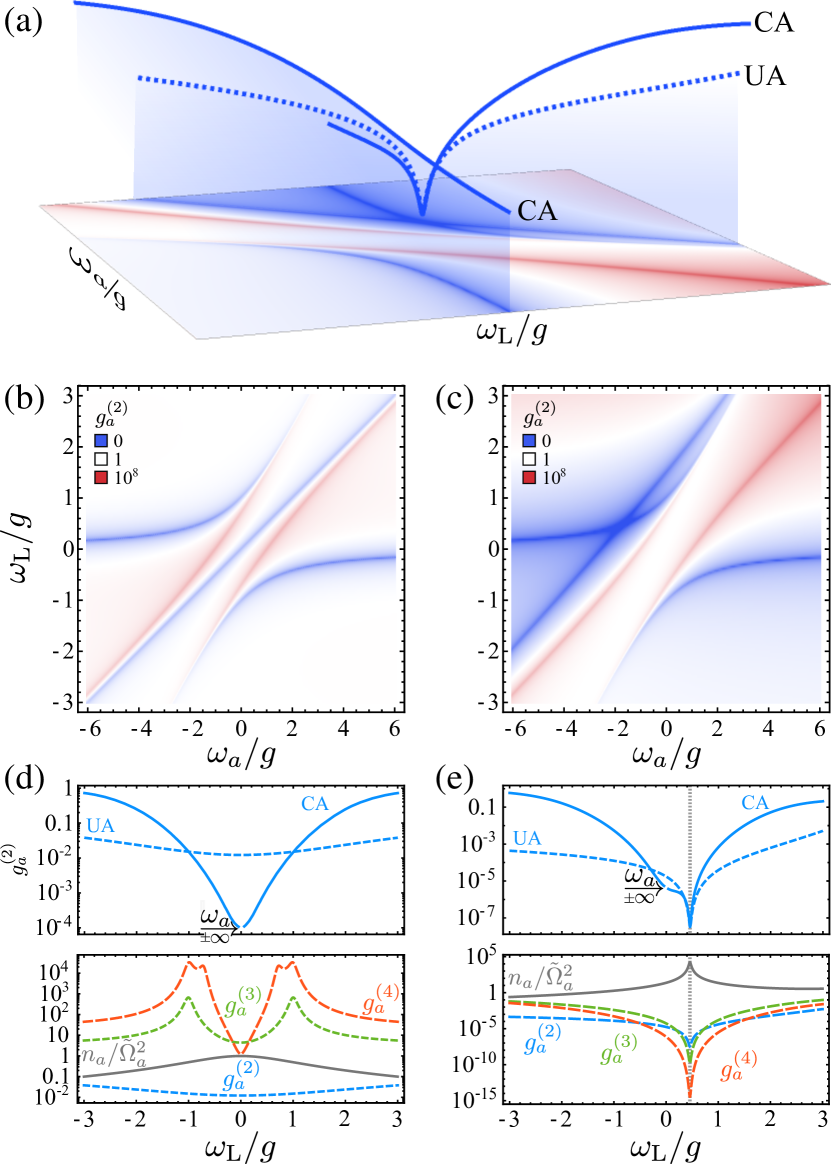
Figure 8: (Color online) Intersection of the UA and CA lines in the Jaynes–Cummings model. (a) Representation to show simultaneously the lines’ shape in the correlation landscape and their magnitude, with two of them intersecting with the effect of the UA line dragging down the CA line. (b–c) Correlation landscapes with (b) no intersection, when $\chi=0.87$ and $\phi=\pi$ and (c) [case also shown in (a)] with intersection, when $\chi=0.5$ and $\phi=\pi/2$. (d–e) Magnitude of the UA and CA along their respective lines, as a function of $\omega_{\mathrm{L}}$ as the scanning parameter. Note that, as a consequence, the case $\omega_{\mathrm{L}}=0$ corresponds to infinite cavity detuning, indicated by a gap opening which is otherwise continuous. In the intersecting case, note the highly populated, strong and all-order antibunching. Parameters are the same as in Fig. 5(a).

In this case, one can find the peculiar situation where conventional and unconventional features intersect. This can happen for the superbunching as seen in Fig. 5(a), with the effect of maximizing it drastically when UB and CB meet, but more notably, it can also happen involving a polariton line, meaning, with a lot of signal. Namely, the CA from the upper polariton branch can meet the UA line, as shown in Fig. 8 that compares the case of balanced driving, namely, $\Omega_{a}=\Omega_{\sigma}$ ($\chi=1$) with both $\rightarrow 0$ (left column), with unbalanced driving, $\Omega_{a}\approx\Omega_{\sigma}/5$ ($\chi\approx 5$), and going to zero in this ratio. In the correlation-landscapes, one can recognize the CA polariton lines, displaying the characteristic anticrossing shapes, and the straight line of UA (all in blue, being antibunched). In the $\chi=0$ case, the UA line fits between the two CA line and all remain distinct. In the $\chi=0.87$ case, the UA line is shifted to negative $\omega_{a}$ and intersects the CA line (at $\omega_{a}\approx-1.73g$ and $\omega_{\mathrm{L}}\approx 0.46g$). At this intersection, one finds the advantageous configuration combining the best of two worlds, namely, a large population since the emission comes from a real state of the system (CA), the antibunching is very strong (UA) and occurs to all-orders (CA). This is shown in Panels (d–e) of Fig. 8. In the non-intersecting case (left column), antibunching is better (smaller) in the CA case when $|\omega_{\mathrm{L}}|<g$, because self-homodyning, with $g^{(2)}_{a}(\mathrm{UA})\approx 0.012$, happens in this case to be far from its optimum cancellation, and by symmetry, also have its minima degenerate, thus bearing resemblances, although superficially only, with conventional antibunching. One features that remains is the small population, namely, $n_{a}/\tilde{\Omega}_{a}^{2}\approx 0.99$. Although CA is better in this case, it reaches its minimum of $g^{(2)}_{a}(\mathrm{CA})\approx 10^{-4}$ when $\omega_{a}\rightarrow\pm\infty$, so this is an asymptotic optimum (which we indicate on the figure by opening a gap in the curve pointed out by $\mathrel{\begin{subarray}{c}\omega_{a}\\ \longrightarrow\\ \pm\infty\end{subarray}}$). Now, comparing with the intersecting case (right column), the UA exhibits one of its typical sharp and strong resonances, here with $g^{(2)}_{a}\approx 3.3\times 10^{-8}$, and this drags the CA line in its wake, as seen in Fig. 8(a) in the full-space of correlation and more quantitatively in Fig. 8(e). Also, all the $n$-photon antibunching are now degenerate, as is typical of a CA resonance. And as the final asset, the population is, this time, $n_{a}/\tilde{\Omega}_{a}^{2}\approx 1.67\times 10^{4}$, that is, almost 20 000 times higher than in the non-intersecting case. We have, therefore, a considerably enhanced situation due to the intersection of UA and CA lines: a much stronger antibunching as compared to CA alone, with a much stronger signal as compared to UA alone. We further discuss this peculiarity in the next section, where it becomes even more attractive. We conclude this section by noting that the $\mathrel{\begin{subarray}{c}\omega_{a}\\ \longrightarrow\\ \pm\infty\end{subarray}}$ gap opened in the CA line does not produce a discontinuity, suggesting underlying symmetries and a peculiar parameter-space topology supporting the landscape of correlations, which we are simply laying down on a plane for simplicity and by force of habit, but such a continuity, which becomes compelling in absence of a symmetry as in Fig. 8(e), points at a better parametrization.

VII Microcavity polaritons statistics

We now contrast the previous results with a platform—namely, microcavity polaritons—where the effects just discussed become even more relevant given the intense activity in realizing the two types of antibunching: conventional and unconventional. We will show in particular how the rich interplay of self-homodyning of the anharmonic oscillator Zubizarreta Casalengua et al. (2020) with a cavity leads to surprising results going against the community’s expectations regarding the role of interactions and the experimental configurations to consider. The Hamiltonian is similar to the Jaynes–Cumming’s Eq. (53), except that the emitter (excitons) has annihilation operator $b$ also following Bose algebra (like $a$) but with a nonlinear quartic nonlinearity of strength $U$ (describing exciton-exciton self-interactions):

$$H={} \hbar\omega_{a}{a^{\dagger}}a+\hbar\omega_{b}{b^{\dagger}}b+\frac{U}{2}{b^{\dagger}}{b^{\dagger}}bb+\hbar g({a^{\dagger}}b+a{b^{\dagger}})+{}$$

$$+\Omega_{a}e^{i\omega_{a}t}a+\Omega_{b}e^{i\omega_{b}t}b+\mathrm{h.c.}$$ (66)

In the limit $U\rightarrow\infty$, the results recover those of the Jayne–Cummings model. Polariton systems have weak nonlinearities $U\ll\gamma_{a}$ and we will consider both limits. The antibunching for both the cavity and exciton emission (since this is one is not trivially zero anymore) can be obtained in closed-form. Again, despite the result not being of immediate interest in such a bulky form, given that it covers in a unified single-formula a plethora of results that one otherwise finds scattered in the literature, we nevertheless give it in its entirety as follows:

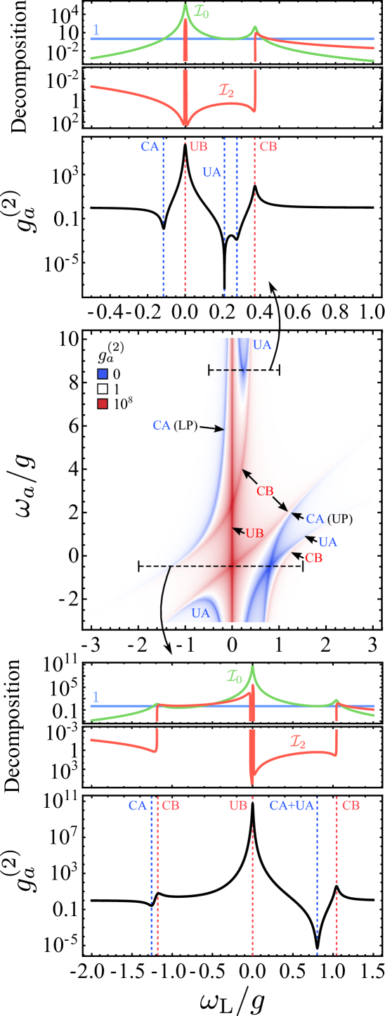
Figure 9: (Color online) Decomposition of $g^{(2)}_{a}$ in terms of the $\mathcal{I}$ coefficients (Supplemental Material), for microcavity polaritons, along the two cuts shown in the central panel, which intersect the points where $g^{(2)}_{a}$ becomes exactly zero to leading order for the upper cut and corresponds to the CA–UA intersection point for the lower cut. Parameters: $g=1$, $\gamma_{a}=0.1$, $\gamma_{b}=0.01$, $U=1$, $\chi=0$ ($\phi=0$). The cuts are at $\omega_{a}/g\approx 8.63$ where UA is exactly zero and $\omega_{a}/g\approx-0.44$ where UA and CA intersect.

$$\begin{split}g^{(2)}_{a}=&\Big{\{}\Big{[}16g^{4}+8g^{2}\big{(}\gamma_{a}\gamma_{b}-4\Delta_{a}\Delta_{b}\big{)}+\Gamma_{a}^{2}\Gamma_{b}^{2}\Big{]}\Big{[}\Gamma_{b}^{2}\Gamma_{11}^{2}\big{(}\gamma_{b}^{2}+\tilde{U}_{12}^{2}\big{)}+8g^{2}\Big{(}U^{2}[4\Delta_{b}\tilde{\Delta}_{11}-\gamma_{b}\tilde{\gamma}_{11}]+2\Gamma_{11}^{2}[\gamma_{b}^{2}+\tilde{U}_{12}^{2}]\chi^{2}+\\ &8U\Delta_{b}^{2}\tilde{\Delta}_{11}-2U\gamma_{b}^{2}\tilde{\Delta}_{13}-4U\gamma_{a}\gamma_{b}\Delta_{b}\Big{)}+16g^{4}\Big{(}U^{2}+[\tilde{\gamma}_{11}^{2}+(U+2\tilde{\Delta}_{11})^{2}]\chi^{4}\Big{)}-16g\chi\cos\phi\,\Big{(}\Delta_{b}\Gamma_{11}^{2}[\gamma_{b}^{2}+\tilde{U}_{12}^{2}]\\ &+2g^{2}[U(2\tilde{\Delta}_{11}\tilde{U}_{12}-\gamma_{b}\tilde{\gamma}_{11})+(2U^{2}\tilde{\Delta}_{11}+2\Delta_{b}\Gamma_{11}^{2}+U\{\gamma_{a}\tilde{\gamma}_{11}+4\tilde{\Delta}_{11}\tilde{\Delta}_{12}\})\chi^{2}]\Big{)}+8g^{2}\chi^{2}\cos 2\phi\,\Big{(}4g^{2}U[U+2\tilde{\Delta}_{11}]-\\ &U^{2}[\gamma_{b}\tilde{\gamma}_{11}-4\Delta_{b}\tilde{\Delta}_{11}]-[\gamma_{b}^{2}-4\Delta_{b}^{2}]\Gamma_{11}^{2}+2U[\gamma_{a}^{2}\Delta_{b}+\tilde{\Delta}_{12}(4\Delta_{b}\tilde{\Delta}_{11}-\gamma_{b}^{2})]\Big{)}-8g\chi\sin\phi\,\Big{(}\gamma_{b}\Gamma_{11}^{2}[\gamma_{b}^{2}+\tilde{U}_{12}^{2}]+\\ &4g^{2}[\gamma_{b}\Gamma_{11}^{2}\chi^{2}+U(\chi^{2}-1)(U\tilde{\gamma}_{11}+2\gamma_{b}\Delta_{a}+2\tilde{\gamma}_{12}\Delta_{b})]\Big{)}+8g^{2}\chi^{2}\sin 2\phi\,\Big{(}-4g^{2}U\tilde{\gamma}_{11}+4\gamma_{b}\Delta_{b}\Gamma_{11}^{2}+2U^{2}[\gamma_{a}\Delta_{b}+\gamma_{b}\tilde{\Delta}_{12}]+\\ &U[\gamma_{a}^{2}\gamma_{b}+4\gamma_{b}\tilde{\Delta}_{12}^{2}+\gamma_{a}\Gamma_{b}^{2}]\Big{)}\Big{]}\Big{\}}\Big{/}\Big{\{}\Big{(}\Gamma_{a}^{2}\Gamma_{11}^{2}\big{[}\gamma_{b}^{2}+\tilde{U}_{12}^{2}\big{]}+16g^{4}\big{[}\tilde{\gamma}_{11}^{2}+\big{(}U+2\tilde{\Delta}_{11}\big{)}^{2}\big{]}+8g^{2}\big{[}U^{2}\big{(}\gamma_{a}\tilde{\gamma}_{11}-4\Delta_{a}\tilde{\Delta}_{11}\big{)}+{}\\ &\Gamma_{11}^{2}\big{(}\gamma_{a}\gamma_{b}-4\Delta_{a}\Delta_{b}\big{)}-2U\big{(}\gamma_{a}^{2}\tilde{\Delta}_{1\bar{1}}-2\gamma_{a}\gamma_{b}\Delta_{b}+4\Delta_{a}\tilde{\Delta}_{11}\tilde{\Delta}_{12}\big{)}\big{]}\Big{)}\Big{(}4g^{2}\chi^{2}+\Gamma_{b}^{2}-4g\chi\big{[}2\Delta_{b}\cos\phi+\gamma_{b}\sin\phi\big{]}\Big{)}^{2}\Big{\}}\,,\end{split}$$ (67a)

$$\begin{split}g^{(2)}_{b}=&\big{\{}\Gamma_{11}^{2}\big{[}16g^{4}+8g^{2}\big{(}\gamma_{a}\gamma_{b}-4\Delta_{a}\Delta_{b}\big{)}+\Gamma_{a}^{2}\Gamma_{b}^{2}\big{]}\big{\}}\Big{/}\big{\{}\Gamma_{a}^{2}\Gamma_{11}^{2}\big{[}\gamma_{b}^{2}+\tilde{U}_{12}^{2}\big{]}+16g^{4}\big{[}\tilde{\gamma}_{11}^{2}+\big{(}U+2\tilde{\Delta}_{11}\big{)}^{2}\big{]}+{}\\ &8g^{2}\big{[}U^{2}\big{(}\gamma_{a}\tilde{\gamma}_{11}-4\Delta_{a}\tilde{\Delta}_{11}\big{)}+\Gamma_{11}^{2}\big{(}\gamma_{a}\gamma_{b}-4\Delta_{a}\Delta_{b}\big{)}-2U\big{(}\gamma_{a}^{2}\tilde{\Delta}_{1\bar{1}}-2\gamma_{a}\gamma_{b}\Delta_{b}+4\Delta_{a}\tilde{\Delta}_{11}\tilde{\Delta}_{12}\big{)}\big{]}\big{\}}\,,\end{split}$$ (67b)

where we have used the short-hand notation $\Gamma_{c}^{2}=\gamma_{c}^{2}+4\Delta_{c}^{2}$ for $c=a,b$ as well as $\tilde{\Delta}_{ij}\equiv i\Delta_{a}+j\Delta_{b}$, $\tilde{\gamma}_{ij}\equiv i\gamma_{a}+j\gamma_{\sigma}$, $\Gamma_{ij}^{2}\equiv\tilde{\gamma}_{ij}^{2}+4\tilde{\Delta}^{2}_{ij}$, $\tilde{U}_{ij}\equiv iU+j\Delta_{b}$ and $\bar{j}$ denotes negative integer values ($\bar{j}\equiv-j$). As before, considerable simplifications are obtained when focusing on particular cases, e.g., by considering cavity pumping only, i.e., $\chi=0$ (the case usually assumed in the literature), in which case, Eq. (67a) reduces to

$$g^{(2)}_{a}=[16g^{4}+8g^{2}(\gamma_{a}\gamma_{b}-4\Delta_{a}\Delta_{b})+\Gamma_{a}^{2}\Gamma_{b}^{2}]\times{}\\ {}\times\{16g^{4}U^{2}+\Gamma_{b}^{2}\Gamma_{11}^{2}[\gamma_{b}^{2}+(U+2\Delta_{b})^{2}]-8g^{2}U[4\gamma_{a}\gamma_{b}\Delta_{b}-8\Delta_{b}^{2}\Delta_{11}+2\gamma_{b}^{2}(\Delta_{11}+2\Delta_{b})+U(\gamma_{b}\gamma_{11}-4\Delta_{b}\Delta_{11})]\}\bigm{/}\\ \big{[}8g^{2}\Gamma_{b}^{4}\{U^{2}(\gamma_{a}\gamma_{11}-4\Delta_{a}\Delta_{11})+\Gamma_{11}^{2}(\gamma_{a}\gamma_{b}-4\Delta_{a}\Delta_{b})-2U[\gamma_{a}^{2}\Delta_{1\bar{1}}-2\gamma_{a}\gamma_{b}\Delta_{b}+4\Delta_{a}\Delta_{11}\Delta_{12}]\}+{}\\ \Gamma_{b}^{4}\{\Gamma_{a}^{2}\Gamma_{11}^{2}[\gamma_{b}^{2}+(U+2\Delta_{b})^{2}]+16g^{4}[\gamma_{11}^{2}+(U+2\Delta_{11})^{2}]\}\big{]}\,.$$ (68)

The same decomposition of this two-photon correlation function can be made in terms of the $\mathcal{I}$ parameters (11). These results are also exact but become extremely heavy even for the particular case $\chi=0$, so we give them in the Supplementary Material. They are plotted for two cuts of interest in the landscape of correlations of polaritons in Fig. 9. We need not describe in much details the structure of this landscape for polaritons since it is so closely related to the Jaynes–Cummings case, with Conventional C and Unconventional U, Bunching B and Antibunching A combinations giving rise to CB, CA, UB and UA lines, with the same origins and consequently identical properties, such as C lines being attributable to dressed states of the systems and U lines to interferences at a given photon number. These are labelled directly on the figure and one can compare with Figs. 5–7 from the Jaynes–Cummings limit to see both similarities and departures. Some are quantitative only, such as the two CB lines that were two parallel lines in the Jaynes–Cummings case now become curved and drifting away in the UP region, where the UA line also gets squeezed and sent away to large cavity detunings. Other are qualitative, like the apparition of a new CB line, due to a dressed state from the second manifold (purely upper-polaritonic) whose energy grows like the interaction strength, being sent away to infinity in the Jaynes–Cummings limit $U\rightarrow\infty$ where the line has thus completely disappeared. The decomposition in terms of the $\mathcal{I}$ parameters also presents mainly quantitative departures from its Jaynes–Cummings counterpart. The strong oscillations of $\mathcal{I}_{2}$ are concomitant with the intersection of the CB and UB lines here, which produces, like in the Jaynes–Cummings case, a boost of superbunching by several orders of magnitudes, peaking at $g^{(2)}_{a}\approx 6.9\times 10^{10}$ for the lower intersection. More importantly, we find again the intersection between the UA and CA lines, already discussed in the previous section. Here, an important deviation is that this can happen without the need of mixed-driving, which is understandably a complication to implement experimentally. Beside in the polariton platform even more so than in the Jaynes–Cummings system, one is interested in finding the optimum antibunching (i.e., smallest $g^{(2)}_{a}$) Sanvitto et al. (2019). The value of this intersection point in this regard will be stressed in the following. As previously, the perfect-antibunching conditions can be derived from the equation $g^{(2)}_{a}=0$, which we will do here for the $\chi=0$ case given by the expression Eq. (68). Then, clearing $\Delta_{a}$ from the previous equation, leads to:

$$\Delta_{a}=\big{\{}e^{i\phi}\big{[}4g^{2}U-\big{(}\gamma_{b}+2i\Delta_{b}\big{)}\big{(}\tilde{\gamma}_{11}+2i\Delta_{b}\big{)}\big{(}U+2\Delta_{b}-i\gamma_{b}\big{)}\big{]}\\ +4ig\chi\big{(}U+2\Delta_{b}-i\gamma_{b}\big{)}\big{(}\tilde{\gamma}_{11}+2i\Delta_{b}\big{)}\\ +4e^{-i\phi}g^{2}\chi^{2}\big{(}U+2\Delta_{b}-i\tilde{\gamma}_{11}\big{)}\big{\}}/\mathcal{N}$$ (69)

where $\mathcal{N}$ is defined as

$$\mathcal{N}=2\big{[}e^{i\phi}\big{(}\gamma_{b}+2i\Delta_{b}\big{)}\big{(}\gamma_{b}+iU+2i\Delta_{b}\big{)}\\ +4g\chi\big{(}U+2\Delta_{b}-i\gamma_{b}\big{)}-4g^{2}\chi^{2}e^{-i\phi}\big{]}.$$ (70)

Again, although by definition $\Delta_{a}$ must be real, we arrive to a complex-valued condition, but the real part of Eq. (69) gives the equation for the UA lines. Moreover, the cancellation of its imaginary part also provides a second condition that allows to identify $g^{(2)}_{a}=0$ exactly, to lowest-order in the driving. Like in the Jaynes–Cummings case, since there are two conditions, it is not possible to fulfil both simultaneously except at isolated points in the parameter space. As an illustration, we present here the case of cavity excitation ($\chi=0$). Splitting both real and imaginary parts from Eq. (69), we find:

$$\Delta_{a}=-\Delta_{b}-\frac{4g^{2}\Delta_{b}}{\gamma_{b}^{2}+4\Delta_{b}^{2}}+\frac{2g^{2}(U+2\Delta_{b})}{\gamma_{b}^{2}+(U+2\Delta_{b})^{2}}\,,$$ (71a)

$$0=\gamma_{a}+\gamma_{b}+4g^{2}\gamma_{b}\left(-\frac{1}{\gamma_{b}^{2}+4\Delta_{b}^{2}}+\frac{1}{\gamma_{b}^{2}+(U+2\Delta_{b})^{2}}\right).$$ (71b)

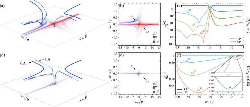
Figure 10: (Color online) Conventional and unconventional statistics in a microcavity polariton system, with strong (top row, $U/\gamma_{a}=0.2$) and weak (bottom row, $U/\gamma_{a}=0.03$) interactions. (a, d) Conventional (solid) and unconventional (dashed) antibunching as a 3D representation of the landscapes of correlations shown in panels (b–e). Note how the CA line gets pulled down by the UA one if they intersect. (c–f) $g^{(n)}_{a}$ for $n=2,3,4$ along the upper (UP) and lower (LP) polariton lines (i.e., CA). The upper polariton line gets a much better antibunching thanks to its proximity, or even intersection, with the unconventional antibunching. The inset in panel (f) shows for comparison the much smaller antibunching of the upper line (the one so far reported experimentally).

The first expression, Eq. (71a), provides an implicit equation for the three distinct curves of UA shown in Figs. 9 and 10, whereas the latter gives the exact location where $g^{(2)}_{a}$ becomes exactly zero, to lowest-order in the driving.

To appreciate how these several aspects compete with each others, we show in Fig. 10(a,d) a 3D representation of the joint magnitude and shapes of the antibunching lines in the polaritonic landscapes of correlations, for strong (upper row) and weak (lower row) polariton interactions. The correlation landscapes are also shown in Panels (b) and (e) with the two polariton branches identified, and the magnitudes of antibunching on the polariton branches are given up to the fourth-order in Panels (c) and (f). There is a crossing of the CA and UA lines in the upper case, as indeed the conditions for the intersection to take place require that the interactions $U$ are neither too large nor too weak but be in the range

$$2.57\gamma_{b}+9.30\gamma_{b}^{3}/g^{2}\lesssim U\lesssim 2(g^{2}/\gamma_{b})-5\gamma_{b}$$ (72)

which is obtained by studying the solutions of $\mathrm{UA}=\mathrm{CA}$ in the limit of small $\gamma_{b}$, yielding exact but surprisingly awkward solutions for the lower bound: for instance $2.57$ is really $\sqrt{1+6\cos(\pi/9)}$. The exact solution for 9.30 is a similar but more complex expression in terms of trigonometric functions of multiples of $\pi/9$. When the intersection exists, as is clear in Panel (b) of Fig. 10, one sees (Panels (a) and (c)) how the CA line, typically of fairly modest antibunching, gets sucked-in by the UA line and exhibits, as a result, record-value of antibunching as compared to typical CA values, here with $g^{(2)}_{a}\approx 9.2\times 10^{-6}$, as compared to $g^{(2)}_{a}\approx 0.02$ only on the other (LP) polariton branch. Note, interestingly, that this effect takes place on the UP polariton branch, which is typically discarded by experimentalists for practical reasons (it is typically less bright and not as defined as its lower sister). In both cases, being on the branches, the population is very large, namely, $n_{a}/\tilde{\Omega}_{a}^{2}\approx 31.05$ on the UP as compared to $n_{a}/\tilde{\Omega}_{a}^{2}\approx 0.02$ for the optimum UA off-branch, even though in this case the antibunching is perfect, being exactly zero. Also, although the minima for higher-order correlators are not degenerate with this crossing point, they are at least also very small, unlike UA features alone where two-photon antibunching comes with higher-order photon bunching (cf. Fig. 4).

Although the intersection is not always guaranteed, it is interesting that the proximity alone of the UA and CA lines tends to produce a similar result of a considerable improvement of the CA. This is shown in the bottom row of Fig. 10, where there is no intersection, but as the two lines converge asymptotically towards each other with increasing cavity (negative) detuning, the CA on the UP line becomes much smaller than would be expected from conventional polariton blockade. With $U/\gamma_{a}=0.03$, which is about the experimental value assumed in several systems, this proximity leads to a value of $g^{(2)}_{a}\approx 0.499$ which, to be appreciated, has to be compared with its pure CA counterpart (on the LP branch), which is $g^{(2)}_{a}\approx 0.993$ only, that corresponds to the results recently experimentally reported Muñoz-Matutano et al. (2019); Delteil et al. (2019). Our picture shows the considerable antibunching improvement that is in principle within reach merely by changing branches. The large detuning required to reach the minimum, namely for our parameters, $\omega_{a}\approx-83.4g$, means a smaller population, which can become as detrimental to the signal as being off-branch, and indeed, $n_{a}/\tilde{\Omega}_{a}^{2}\approx 5\times 10^{-4}$ on the highly-detuned UP branch is much less than $n_{a}/\tilde{\Omega}_{a}^{2}\approx 0.02$ for the optimum UA of $g^{(2)}_{a}=0$, off-branch at $\omega_{a}\approx-0.48g$. But since the resonance is very broad, one can still obtain sizable all-order antibunching on the UP branch at smaller detunings, as seen in Fig. 10(f). For instance, at $\omega_{a}=-10g$, a routine-detuning, $g^{(2)}_{a}\approx 0.86$, which would be a clear-cut, compelling measurement still over 20 times larger than the CA on the LP branch, and with, this time, the considerable population $n_{a}/\tilde{\Omega}_{a}^{2}\approx 3.2$, that is about 160 higher than the off-branch UA. At $\omega_{a}=-5g$, with a still neatly-resolvable $g^{(2)}_{a}\approx 0.92$ (similar to the values actually reported in the literature on the lower branchMuñoz-Matutano et al. (2019); Delteil et al. (2019)), one gains another order of magnitude in signal.

We leave these interesting prospects of this intersection for an even more surprising result, that concerns the strength of the interactions required to optimize antibunching. It is widely assumed that as strong as possible interactions are required to maximise antibunching (i.e., to minimise the value of $g^{(2)}_{a}$). This is true for CA, but not for UA. Consequently, this limitation also gets lifted at the UA–CA intersection, with an antibunching on the polariton branch, with a large population that is maximum for a finite interaction strength, close to $U\approx g$. This coincidental value appears to be favouring the level degeneracy and thus to optimize the unconventional type of the joint antibunching. This is shown in Fig. 11(a), that provides the optimum two-photon antibunching $g^{(2)}_{a}$ along the LP line (black), where it is purely CA, and along the UP line (red), where it intersects with the UA line. The LP antibunching behaves as expected, steadily decreasing until it reaches its optimum value which is that of the Jaynes–Cummings system when $U\rightarrow\infty$, with $g^{(2)}_{a}\approx 4.4\times 10^{-3}$. In contrast, the UP antibunching achieves several orders of magnitude smaller values for finite interactions, namely, $g^{(2)}_{a}\approx 3.5\times 10^{-6}$ at $U/\gamma_{a}\approx 4.8$. While this optimum antibunching is obtained for a very strong interaction strength by today’s polaritonic standards, one still get a considerable improvement for the typical values of current experiments, as shown in Panel (b). We already discussed the case $U/\gamma_{a}=0.03$, that is shown again with the strong-interaction case $U/\gamma_{a}=2$ in Panel (c), where one sees how the LP optimum antibunching (shown with the dotted vertical grey line) arises from the UA–CA intersection in the strongly-interacting case and the pull-down effect from their proximity in the low-interaction one. The detuning that minimizes $g^{(2)}_{a}$ on the UP line, that is, where to drive the system to optimize its bright antibunched emission, is shown in in Panel (d). Here again, one can compromise antibunching for a stronger signal by reducing the detuning. More than the antibunching per se, these results could be particularly attractive to accurately estimate the strength of polariton interactions.

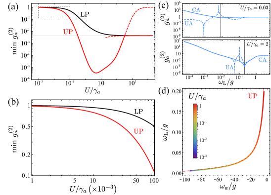
Figure 11: (Color online) Polariton antibunching as a function of polariton interactions. (a) Antibunching on the two polariton branches, showing the much greater UP antibunching due to the proximity to the UA line, even at very small interactions (zoom in Panel (b)). An optimum is obtained for a finite value of interactions, in contrast to antibunching on the LP line which is optimum in the Jaynes–Cummings limit $U\rightarrow\infty$. The solid lines in (a) show the optimum value of $g^{(2)}_{a}$ on the LP (black) and the UP (red). On the UP, where it is significantly stronger, this is due to the intersection, or proximity, between UA and CA, until interactions get very large, $U/\gamma\gtrsim 10$, where another local minimum overtakes and the UA+CA carries on as the dashed line. (c) Details of the proximity (top) and intersection (bottom) effect for the small and high interactions, respectively. The vertical line shows the minimum antibunching on the UP line, which is CA. (d) Location on the UP line where to drive the system depending on its interaction $U/\gamma_{a}$ to optimize its two-photon antibunching.

We conclude with a brief consideration on the role of dephasing on the effects we have discussed in this text. Although they also are of a general character, we discuss them in the context of polaritons only. Pure dephasing can be included to a system’s dynamics by adding to the master equation the Lindblad term $(\gamma_{\phi}/2)\mathcal{L}_{{b^{\dagger}}b}\rho$ with $\gamma_{\phi}$ the dephasing rate. This describes loss of quantum coherence, and has the overall effect of spoiling correlations: damping superbunching and antibunching, both getting closer to 1 from their respective sides of $g^{(2)}=1$. This affects as well our homodyning configuration, where we can restore or impose infinite superbunching and exactly zero antibunching to leading-order in the driving, in absence of dephasing. This becomes impossible when $\gamma_{\phi}\neq 0$, even in the vanishing driving regime López Carreño et al. (2019). On the other hand, the response of conventional and unconventional features to dephasing is very different, confirming their distinct nature and character. Namely, conventional features are much less sensitive to dephasing and remain mostly undisturbed for small values of dephasing as compared to the linewidths of the bare states, i.e., when $\gamma_{\phi}/\gamma_{b}\lesssim 1$ Zubizarreta Casalengua et al. (2020). Above that point, corresponding to considerable dephasing rates, conventional features start to fade away although slowly and still exhibiting a remarkable resilience. In comparison, unconventional features, which are due to interferences, are extremely fragile and their very-good values without dephasing are strongly affected by its presence. The behaviour of the intersection of CA and UA is interesting in this regard. Panel (d) of Fig. 12 shows the evolution of $g^{(2)}_{a}$ for three types of antibunching: $(i)$ the intersection of UA and CA, identified by a circle in Fig. 12(b), and $(ii)$ the CA, and $(iii)$ the UA on the cut (c). One can see, again, how CA is more robust to dephasing, remaining essentially unaffected till $\gamma_{\phi}$ becomes a significant fraction of $\gamma_{b}$. In contrast, UA is quickly spoiled by $\gamma_{\phi}$. Interestingly, the intersection behaves like both types, being strongly affected when it is very small and exhibiting the same type of resilience to dephasing as CA when its antibunching becomes of the same magnitude.

Another interesting role of dephasing goes beyond affecting the existing features, and brings new ones, namely, additional bunching resonances appear with $\gamma_{\phi}\neq 0$, which could also be considered for spectroscopic applications so as to estimate the amount of dephasing present in a system. This is shown in Fig. 12, where the correlation landscape is shown for a small dephasing rate ($\gamma_{\phi}/g=0.1\gamma_{b}$). Arrows point at the two new lines that are dephasing-induced. They are also shown in two cuts at $\omega_{a}/g=-3$ and $\omega_{a}/g=8$, in Panels (a) and (c), that compare the case with (dark-blue) and without (light-blue) dephasing. The additional bunching peaks correspond to transitions between polariton energy levels. Consequently, the line I (at negative detunings) fulfills

$$\omega_{\mathrm{L}}=\tilde{E}_{0}^{(2)}-\tilde{E}_{-}^{(1)}$$ (73)

while line II (at positive detunings) is given by

$$\omega_{\mathrm{L}}=\tilde{E}_{-}^{(2)}-\tilde{E}_{-}^{(1)}\,,$$ (74)

where $\tilde{E}^{(k)}_{l}$ are the energy levels of the few-particle (up to $k=2$) polariton states, which can be obtained in closed-form but yielding awkward expressions. We give here the first-order term in the interaction $U$ under strong-coupling conditions ($g\gg\gamma_{a}$, $\gamma_{b}$):

$$\tilde{E}_{0}^{(2)} =\omega_{a}+\omega_{b}+\frac{g^{2}}{2R^{2}}U\,,$$ (75a)

$$\tilde{E}^{(2)}_{\pm} =\omega_{a}+\omega_{b}\pm 2R{}$$

$$\quad{}+\frac{2g^{2}+(\omega_{a}-\omega_{b})[(\omega_{a}-\omega_{b})\mp 2R]}{8R^{2}}U\,,$$ (75b)

with $R=\sqrt{g^{2}+(\omega_{a}-\omega_{b})^{2}/4}$, and $\tilde{E}_{-}^{(1)}=E_{-}^{(1)}$ of Eq. (57) since in absence of interactions and transitions, the lower-polariton energies coincide with the one-polariton excitations. One polariton, from the upper or lower branch, is emitted, leaving some room for a second polariton to be radiated. The incoherent contribution to the field is no longer depleted to second-order, whence the origin of these transitions.

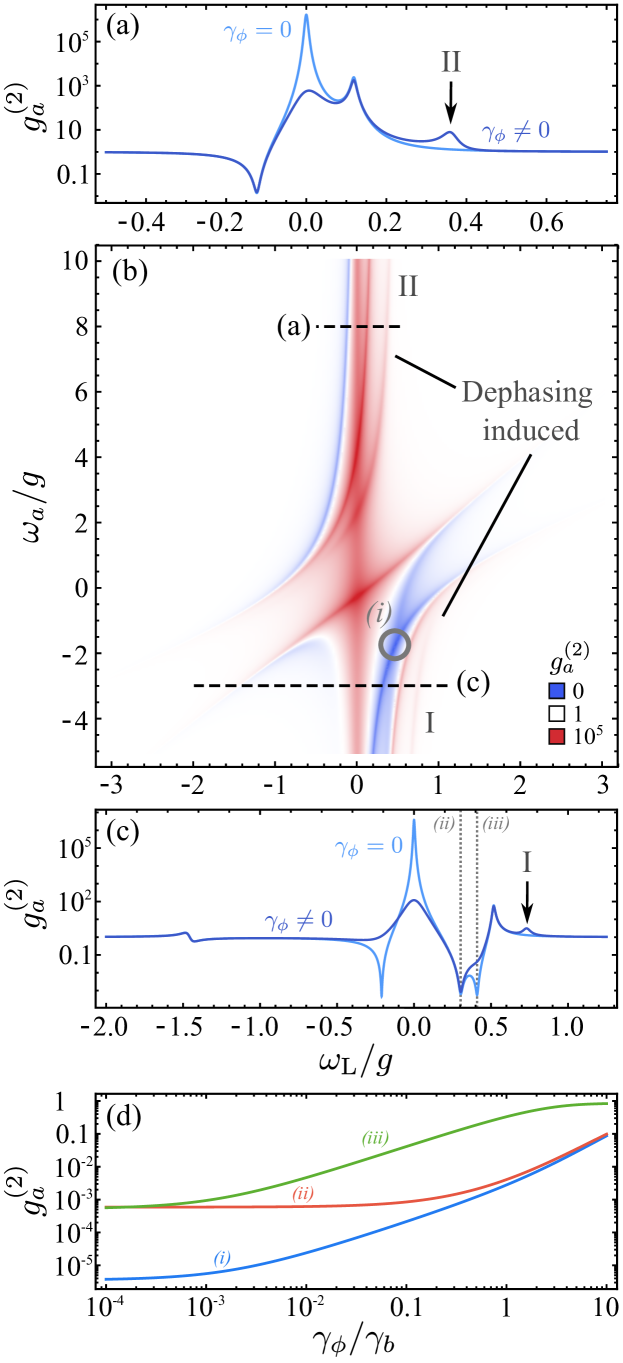
Figure 12: Effect of dephasing on photon correlations $g^{(2)}_{a}$. In Panel (b), the correlation landscape scanning in frequencies, with two cuts shown in Panels (a) and (c) at $\omega_{a}/g=-3$ and $8$, respectively, along with their dephasing-free counterparts (light blue). Some of the antibunching/bunching peaks, related to unconventional features, are strongly suppressed whereas conventional lines are left almost untouched. Additionally, new dephasing-induced lines emerge, labelled I and II in (a–c). Panel (d) shows the robustness of the antibunching against dephasing: (i) for the $\mathrm{UA}+\mathrm{CA}$ intersection (marked with a gray circle in Panel (b)), (ii) for CA and (iii) for UA at the position shown in Panel (c). Parameters: $g=1$, $\gamma_{a}=0.1$, $\gamma_{b}=0.01$, $U=0.5$, $\chi=0$ (cavity driven) and $\gamma_{\phi}=0.1\gamma_{b}$.

VIII Summary and Conclusions

If one mixes a coherent state with a quantum state, such as a squeezed state, depending on their relative amplitudes and phases, one can tune the statistics of the resulting state from superbunching to antibunching, although a coherent state has no correlations and a squeezed state is always super-Poissonian. This is the manifestation at the multiphoton level of the well-known “not just the sum” principle of interfering fields, whereby their combination can result in a total that has opposite characteristics. Indeed, bringing the two-photon nonzero amplitudes out of phase will result in two-photon antibunching in the total field, if they otherwise differ in their one and three-photon components, so the effect is, again, neatly produced with a squeezed and coherent states. As amplitudes go to zero, the correlations can actually diverge or vanish completely. This simple phenomenology turns out to be at the foundation of a large body of results in coherently-driven systems, where they have been branded as an “unconventional photon blockade”, in reference to the conventional blockade scenario due to nonlinearities that act as a photon turnstile. This unconventional mechanism produces much stronger correlations and is particularly noteworthy in not relying on strong nonlinearities. For these reasons, it has triggered an intense research activity with a thriving literature Xu and Li (2013); Tang et al. (2015); Shen et al. (2015a, b); Li et al. (2015); Xu et al. (2016); Wang et al. (2016); Zhou and Li (2016); Zhou et al. (2016); Liu et al. (2016); Kryuchkyan et al. (2016); Wang et al. (2017); Cheng et al. (2017); Deng et al. (2017); Yu and Liu (2017); Zhou et al. (2018) that studied considerable variations of the effect at the two-photon level, due to an exaggerated appreciation of $g^{(2)}$ to quantify single-photon emission Grünwald (2019). We have shown how this can be fruitfully understood in several platforms (including resonance fluorescence, the Jaynes–Cummings model and microcavity polaritons) as the simple admixing of a coherent state with a quantum state which, to lowest-order in the driving, is a squeezed state, thereby realizing self-consistently and in a dynamical setting the paradigm of feeding a beam-splitter with a coherent state and a squeezed state, producing a displaced squeezed thermal state on one output port. We have shown in particular how one can control externally the coherent field to tune the statistics of the overall emission. In coherently-driven quantum optical systems, the coherent state does not have to be provided externally but can be seen to come directly from the mean field, while the squeezed state, or other types of quantum states, come from the fluctuations. For given system parameters, a particular configuration of detunings will realize the admixture that yields optimum antibunching and another the optimum superbunching. Scanning over the full range of these parameters, one can thus reveal features in a landscape of correlations, that are clearly explained in terms of the coherent and squeezed states admixture. At low driving, we have shown through a decomposition of the Glauber coherence functions $g^{(n)}$ in terms of coefficients $\mathcal{I}$, $\mathcal{J}$, etc., that embed various types of quantum correlations, how these features are further tightly related to so-called conventional blockade correlations, which pertain to the dressed-states of the system. Since both mechanisms rely on low-driving, even when one is dealing with a two-level system, the driving is too weak to bring the nonlinearity to imprint a non-Gaussian character to the field. Still, both the conventional and unconventional scenarios, that we prefer to tag on the statistics itself rather than on an alleged “blockade,” indeed provide two fairly distinct families of features, with their own characteristics that one can recognise throughout platforms. The two mechanisms combined with the two types of correlations bring us to a classification of UA, UB, CA and CB for Unconventional Antibunching, Unconventional Bunching, Conventional Antibunching and Conventional Bunching, respectively. Their main characteristics are as follows: unconventional features are photon-number dependent, i.e., are realized for a given $n$ that can be chosen, but one at a time, with a typical scenario being a small $g^{(2)}$ but large $g^{(n)}$ for $n\geq 2$, and this takes place in different locations of the parameter space. In contrast, CA occurs to all orders simultaneously and is pinned to the same underlying structure. Unconventional features are typically stronger than conventional ones, also not requiring, as already observed, strong nonlinearities. In the limit of vanishing driving, they become exactly zero (antibunching) and infinite (superbunching) to leading-order in the driving. This manifests itself in much sharper resonances, in particular when contrasted to the conventional ones sitting nearby. But unconventional features are also more fragile, to dissipation, dephasing and driving. Because of the latter, they also suffer from a weak signal. Nonetheless, in the full landscape of correlations, we have shown the existence of intersection points of U and C lines where, remarkably, both qualities of the two types are produced, namely, for the case of antibunching, one can get bright, robust and all-order antibunching, these being features of CA, that is also very strong even in weakly interacting systems, this being the main feature of UA. This is particularly appealing for a platform such as microcavity polaritons, where antibunching is highly sought but remains so-far extremely weak. In the configuration we propose, which involves the upper polariton branch instead of the usually favoured lower one, we predict the existence of a highly-populated, strongly-antibunched emission. While the interest of such a point for applications is unclear given the Gaussian character of the emission, it would certainly be valuable for spectroscopic purposes to help in measuring the polariton-polariton interaction and/or dephasing rate. Overall, at the theoretical level, our picture unifies a considerable amount of phenomenology related to photon statistics in coherently driven systems, which, whether of interest or not for applications, should help be valuable to synthesise the gigantic number of minor variations of a fairly simple theme.

References

- Young (1807) T. Young, A Course of Lectures on Natural Philosophy and the Mechanical Arts (J. Johnson, London, 1807).
- Ficek and Swain (2004) Z. Ficek and S. Swain, Quantum Interference and Coherence: Theory and Experiments (Springer, New York, 2004).
- Ritze and Bandilla (1979) H.-H. Ritze and A. Bandilla, Opt. Commun. 29, 126 (1979).
- Paul (1982) H. Paul, Rev. Mod. Phys. 54, 1061 (1982).
- Bužek and Knight (1995) V. Bužek and P. L. Knight, Progress in Optics 34, 1 (1995).
- Prakash and Mishra (2005) H. Prakash and D. K. Mishra, J. Phys. B.: At. Mol. Opt. Phys. 38, 665 (2005).
- Majumdar et al. (2012) A. Majumdar, D. Englund, M. Bajcsy, and J. Vuc̆ković, Phys. Rev. A 85, 033802 (2012).
- Boddeda et al. (2019) R. Boddeda, Q. Glorieux, A. Bramati, and S. Pigeon, J. Phys. B.: At. Mol. Opt. Phys. 52, 215401 (2019).
- Vogel (1991) W. Vogel, Phys. Rev. Lett. 67, 2450 (1991).
- Vogel (1995) W. Vogel, Phys. Rev. A 51, 4160 (1995).
- Carmichael (1985) H. J. Carmichael, Phys. Rev. Lett. 55, 2790 (1985).
- Fischer et al. (2016) K. A. Fischer, K. Müller, A. Rundquist, T. Sarmiento, A. Y. Piggott, Y. Kelaita, C. Dory, K. G. Lagoudakis, and J. Vuc̆ković, Nature Photon. 10, 163 (2016).
- Müller et al. (2016) K. Müller, K. A. Fischer, C. Dory, T. Sarmiento, K. G. Lagoudakis, A. Rundquist, Y. A. Kelaita, and J. Vučković, Optica 3, 931 (2016).
- Dory et al. (2017) C. Dory, K. A. Fischer, K. Müller, K. G. Lagoudakis, T. Sarmiento, A. Rundquist, J. L. Zhang, Y. Kelaita, N. V. Sapra, and J. Vuc̆ković, Phys. Rev. A 95, 023804 (2017).
- Fischer et al. (2017) K. A. Fischer, Y. A. Kelaita, N. V. Sapra, C. Dory, K. G. Lagoudakis, K. Müller, and J. Vuc̆ković, Phys. Rev. Appl. 7, 044002 (2017).
- Fischer et al. (2018) K. Fischer, S. Sun, D. Lukin, Y. Kelaita, R. Trivedi, and J. Vuc̆ković, Phys. Rev. A 98, 021802(R) (2018).
- Foster et al. (2019) A. Foster, D. Hallett, I. Iorsh, S. Sheldon, M. Godsland, B. Royall, E. Clarke, I. Shelykh, A. Fox, M. Skolnick, I. Itskevich, and L. Wilson, Phys. Rev. Lett. 122, 173603 (2019).
- Zubizarreta Casalengua et al. (2020) E. Zubizarreta Casalengua, J. C. López Carreño, F. P. Laussy, and E. del Valle, Laser Photon. Rev. (2020).
- Lvovsky and Babichev (2002) A. I. Lvovsky and S. A. Babichev, Phys. Rev. A 66, 011801(R) (2002).
- Windhager et al. (2011) A. Windhager, M. Suda, C. Pacher, M. Peev, and A. Poppe, Opt. Commun. 284, 1907 (2011).
- Xu et al. (2012) X. Xu, F. Jia, L. Hu, Z. Duan, Q. Guo, and S. Ma, J. Mod. Opt. 59, 1624 (2012).
- Mehringer et al. (2018) T. Mehringer, S. Mährlein, J. von Zanthier, and G. S. Agarwal, Opt. Lett. 43, 2304 (2018).
- Blaizot and Ripka (1985) J.-P. Blaizot and G. Ripka, Quantum Theory of Finite Systems (MIT Press, Cambridge, MA, 1985).
- Gerry and Knight (2005) C. C. Gerry and P. L. Knight, Introductory Quantum Optics (Cambridge University Press, Cambridge, 2005).
- López Carreño et al. (2018) J. C. López Carreño, E. Z. Casalengua, E. del Valle, and F. P. Laussy, Quantum Science and Technology 3, 045001 (2018).
- Glauber (1963) R. J. Glauber, Phys. Rev. Lett. 10, 84 (1963).
- Mandel (1982) L. Mandel, Phys. Rev. Lett. 49, 136 (1982).
- Mandel (1979) L. Mandel, Opt. Lett. 4, 205 (1979).
- Lemonde et al. (2014) M.-A. Lemonde, N. Didier, and A. A. Clerk, Phys. Rev. A 90, 063824 (2014).
- Liew and Savona (2010) T. C. H. Liew and V. Savona, Phys. Rev. Lett. 104, 183601 (2010).
- Bamba et al. (2011) M. Bamba, A. Ĭmamoḡlu, I. Carusotto, and C. Ciuti, Phys. Rev. A 83, 021802(R) (2011).
- Flayac and Savona (2017) H. Flayac and V. Savona, Phys. Rev. A 96, 053810 (2017).
- Ferretti et al. (2010) S. Ferretti, L. C. Andreani, H. E. Türeci, and D. Gerace, Phys. Rev. A 82, 013841 (2010).
- Flayac and Savona (2013) H. Flayac and V. Savona, Phys. Rev. A 88, 033836 (2013).
- Majumdar and Gerace (2013) A. Majumdar and D. Gerace, Phys. Rev. B 87, 235319 (2013).
- Gerace and Savona (2014) D. Gerace and V. Savona, Phys. Rev. A 89, 031803(R) (2014).
- Flayac et al. (2015) H. Flayac, D. Gerace, and V. Savona, Sci. Rep. 5, 11223 (2015).
- Zhou et al. (2015) Y. H. Zhou, H. Z. Shen, and X. X. Yi, Phys. Rev. A 92, 023838 (2015).
- Tang et al. (2015) J. Tang, W. Geng, and X. Xu, Sci. Rep. 5, 9252 (2015).
- Cheng et al. (2017) X. Cheng, H. Ye, and Z. Yu, Superlatt. Microstruct. 105, 81 (2017).
- Yu and Liu (2017) Y. Yu and H.-Y. Liu, J. Mod. Opt. 64, 1342 (2017).
- Wang et al. (2017) G. Wang, H. Z. Shen, C. Sun, C. Wu, J.-L. Chen, and K. Xue, J. Mod. Opt. 64, 583 (2017).
- Snijders et al. (2018) H. Snijders, J. Frey, J. Norman, H. Flayac, V. Savona, A. Gossard, J. Bowers, M. van Exter, D. Bouwmeester, and W. Löffler, Phys. Rev. Lett. 121, 043601 (2018).
- Vaneph et al. (2018) C. Vaneph, A. Morvan, G. Aiello, M. Féchant, M. Aprili, J. Gabelli, and J. Estève, Phys. Rev. Lett. 121, 043602 (2018).
- Shen et al. (2018) H. Z. Shen, C. Shang, Y. H. Zhou, and X. X. Yi, Phys. Rev. Lett. 98, 023856 (2018).
- Trivedi et al. (2019) R. Trivedi, M. Radulaski, K. A. Fischer, S. Fan, and J. Vuc̆ković, Phys. Rev. Lett. 122, 243602 (2019).
- Birnbaum et al. (2005) K. Birnbaum, A. Boca, R. Miller, A. Boozer, T. Northup, and H. Kimble, Nature 436, 87 (2005).
- Verger et al. (2006) A. Verger, C. Ciuti, and I. Carusotto, Phys. Rev. B 73, 193306 (2006).
- Faraon et al. (2008) A. Faraon, I. Fushman, D. Englund, N. Stoltz, P. Petroff, and J. Vuc̆ković, Nature Phys. 4, 859 (2008).
- Faraon et al. (2010) A. Faraon, A. Majumdar, and J. Vuc̆ković, Phys. Rev. A 81, 033838 (2010).
- Hoffman et al. (2011) A. J. Hoffman, S. J. Srinivasan, S. Schmidt, L. Spietz, J. Aumentado, H. E. Türeci, and A. A. Houck, Phys. Rev. Lett. 107, 053602 (2011).
- Rabl (2011) P. Rabl, Phys. Rev. Lett. 107, 063601 (2011).
- Lang et al. (2011) C. Lang, D. Bozyigit, C. Eichler, L. Steffen, J. M. Fink, A. A. Abdumalikov Jr., M. Baur, S. Filipp, M. P. da Silva, A. Blais, and A. Wallraff, Phys. Rev. Lett. 106, 243601 (2011).
- Müller et al. (2015) K. Müller, A. Rundquist, K. A. Fischer, T. Sarmiento, K. G. Lagoudakis, Y. A. Kelaita, C. S. Muñoz, E. del Valle, F. P. Laussy, and J. Vuc̆ković, Phys. Rev. Lett. 114, 233601 (2015).
- Radulaski et al. (2017) M. Radulaski, K. A. Fischer, K. G. Lagoudakis, J. L. Zhang, and J. Vuc̆ković, Phys. Rev. A 96, 011801(R) (2017).
- Deng et al. (2017) W.-W. Deng, G.-X. Li, and H. Qin, Opt. Express 6, 6767 (2017).
- Sarma and Sarma (2017) B. Sarma and A. K. Sarma, Phys. Rev. A 96, 053827 (2017).
- Ghosh and Liew (2019) S. Ghosh and T. C. Liew, Phys. Rev. Lett. 123, 013602 (2019).
- Delteil et al. (2019) A. Delteil, T. Fink, A. Schade, S. H’́ofling, C. Schneider, and A. Ĭmamoḡlu, Nature Mater. 18, 219 (2019).
- Phillips et al. (2020) C. L. Phillips, A. J. Brash, D. P. S. McCutcheon, J. Iles-Smith, E. Clarke, B. Royall, M. S. Skolnick, and A. M. Fox, arXiv:2002.08192 (2020).
- Hanschke et al. (2020) L. Hanschke, L. Schweickert, J. C. López Carreño, E. Schöll, K. D. Zeuner, T. Lettner, E. Zubizarreta Casalengua, M. Reindl, S. F. Covre da Silva, R. Trotta, J. J. Finley, A. Rastelli, E. del Valle, F. P. Laussy, V. Zwiller, K. Müller, and K. D. Jöns, arXiv:2005.11800 (2020).
- Visser and Nienhuis (1995) P. M. Visser and G. Nienhuis, Phys. Rev. A 52, 4727 (1995).
- López Carreño et al. (2019) J. C. López Carreño, E. Z. Casalengua, F. P. Laussy, and E. del Valle, J. Phys. B.: At. Mol. Opt. Phys. 52, 035504 (2019).
- Jaynes and Cummings (1963) E. Jaynes and F. Cummings, Proc. IEEE 51, 89 (1963).
- Shore and Knight (1993) B. W. Shore and P. L. Knight, J. Mod. Opt. 40, 1195 (1993).
- Zubizarreta Casalengua et al. (2018) E. Zubizarreta Casalengua, J. C. López Carreño, F. P. Laussy, and E. del Valle, “Polariton and jaynes-cummings blockade,” http://demonstrations.wolfram.com/PolaritonAndJaynesCummingsBlockade/ (2018).
- del Valle et al. (2009) E. del Valle, F. P. Laussy, and C. Tejedor, Phys. Rev. B 79, 235326 (2009).
- Laussy et al. (2012) F. P. Laussy, E. del Valle, M. Schrapp, A. Laucht, and J. J. Finley, J. Nanophoton. 6, 061803 (2012).
- Xu and Li (2014) X. Xu and Y. Li, Phys. Rev. A 90, 043822 (2014).
- Sanvitto et al. (2019) D. Sanvitto, F. Laussy, and D. Gerace, Nature Mater. 18, 200 (2019).
- Muñoz-Matutano et al. (2019) G. Muñoz-Matutano, A. Wood, M. Johnson, X. V. Asensio, B. Baragiola, A. Reinhard, A. Lemaitre, J. Bloch, A. Amo, B. Besga, M. Richard, and T. Volz, Nature Mater. 18, 213 (2019).
- Xu and Li (2013) X.-W. Xu and Y.-J. Li, J. Phys. B.: At. Mol. Opt. Phys. 46, 035502 (2013).
- Shen et al. (2015a) H. Z. Shen, Y. H. Zhou, and X. X. Yi, Phys. Rev. A 91, 063808 (2015a).
- Shen et al. (2015b) H. Z. Shen, Y. H. Zhou, H. D. Liu, G. C. Wang, and X. X. Yi, Opt. Express 23, 32835 (2015b).
- Li et al. (2015) J. Li, R. Yu, and Y. Wu, Phys. Rev. A 92, 053837 (2015).
- Xu et al. (2016) X.-W. Xu, A.-X. Chen, and Y. Liu, Phys. Rev. A 94, 063853 (2016).
- Wang et al. (2016) X. Wang, A. Miranowicz, H.-R. Li, and F. Nori, Phys. Rev. A 93, 063861 (2016).
- Zhou and Li (2016) B. Zhou and G. Li, Phys. Rev. A 94, 033809 (2016).
- Zhou et al. (2016) Y. H. Zhou, H. Z. Shen, X. Q. Shao, and X. X. Yi, Opt. Express 24, 17332 (2016).
- Liu et al. (2016) Y.-L. Liu, G.-Z. Wang, Y. Liu, and F. Nori, Phys. Rev. A 93, 013856 (2016).
- Kryuchkyan et al. (2016) G. Y. Kryuchkyan, A. R. Shahinyan, and I. A. Shelykh, Phys. Rev. A 93, 043857 (2016).
- Zhou et al. (2018) Y. H. Zhou, H. Z. Shen, X. Y. Zhang, and X. X. Yi, Phys. Rev. A 97, 043819 (2018).
- Grünwald (2019) P. Grünwald, New J. Phys. 21, 093003 (2019).