Quantum Caging in Interacting Many-Body All-Bands-Flat Lattices

Abstract

We consider translationally invariant tight-binding all-bands-flat networks which lack dispersion. In a recent work [arXiv:2004.11871] we derived the subset of these networks which preserves nonlinear caging, i.e. keeps compact excitations compact in the presence of Kerr-like local nonlinearities. Here we replace nonlinear terms by Bose-Hubbard interactions and study quantum caging. We prove the existence of degenerate energy renormalized compact states for two and three particles, and use an inductive conjecture to generalize to any finite number M of participating particles in one dimension. Our results explain and generalize previous observations for two particles on a diamond chain [Vidal et.al. Phys. Rev. Lett. 85, 3906 (2000)]. We further prove that quantum caging conditions guarantee the existence of extensive sets of conserved quantities in any lattice dimension, as first revealed in [Tovmasyan et al Phys. Rev. B 98, 134513 (2018)] for a set of specific networks. Consequently transport is realized through moving pairs of interacting particles which break the single particle caging.

I Introduction

The study of localization phenomena in systems of interacting particles gave rise to some of most remarkable research streams in condensed matter physics during the past decades. Typically these phenomena arise in the absence of translation invariance, as both the first prediction of single particle localization Anderson (1958); Kramer and MacKinnon (1993) and the finite temperature transition to many-body localized phases of weakly interacting quantum particles Basko et al. (2006); Aleiner et al. (2010) have been obtained in tight-binding networks in the presence of uncorrelated spatial disorder. However, both single and many-body particle localization can be achieved in translationally invariant setups (e.g. see Refs. Pino et al., 2016; Abanin et al., 2019 for discussion on disorder-free many-body localization).

One of the notable examples of single particle localization in translationally invariant lattices are flatband networks – lattices where at least one of the Bloch energy bands is independent of the wave vector (hence, dispersionless or flat). Derzhko et al. (2015); Leykam et al. (2018); Leykam and Flach (2018) Differently from Anderson localization where the disorder turns all the eigenstates exponentially localized, the eigenstates associated to a flat band have strictly compact support spanned over a finite number of unit cells – and therefore they are called compact localized states (CLS). Since their first appearance as mathematical testbeds for ferromagnetic ground states  Mielke (1991); Tasaki (1992) the extension of the flatband concept to novel lattice geometries has been of crucial interest. This gave rise to several generator schemes Dias and Gouveia (2015); Morales-Inostroza and Vicencio (2016); Maimaiti et al. (2017); Röntgen et al. (2018); Toikka and Andreanov (2018); Maimaiti et al. (2019) adopting different principles to design artificial flatband lattices in different spatial dimensions.

If all Bloch bands are flat, then all single particle eigenstates are spatially compact. In this all bands flat (ABF) case, single particle transport is fully suppressed and non-interacting particles remain caged within a finite volume of the system. This caging phenomenon due to the collapse of the Bloch spectrum was originally dubbed Aharonov-Bohm (AB) caging since it emerged from a finetuning of a magnetic field into a time-reversal symmetry invariant case. AB caging has been first introduced in a two-dimensional Dice lattice structure.Vidal et al. (1998) From the first case, the study of this localization has been further extended Douçot and Vidal (2002); Fang et al. (2012a); Longhi (2014); Kibis et al. (2015); Hasan et al. (2016); Zhang and Jin (2020) while experimentally AB caged systems has been realized in photonic lattices Fang et al. (2012b); Mukherjee et al. (2018) and qubits nanocircuits Gladchenko et al. (2009).

Since an ABF model has all bands flat, the system displays time reversal invariance. Therefore there is no need to search for ABF models by detouring via time-reversal broken systems with nonzero magnetic synthetic fluxes or simply magnetic fields, only to re-arrive back to a time-reversal symmetry invariant case. Instead, it is much simpler to finetune time-reversal symmetry invariant tight-binding manifolds in order to isolate the ABF cases. This task was executed in Ref. Danieli et al., 2020a through a set of local unitary detangling transformations and their inverse entangling ones, leading to a generator of ABF models in any lattice dimension with any number of flatbands. The detangled basis is the preferred one for the study of perturbations such as disorder and interactions.

The impact of interactions on caged particles was studied in the 1D Creutz lattice Creutz (1999); Takayoshi et al. (2013); Tovmasyan et al. (2013, 2016); Jünemann et al. (2017); Tovmasyan et al. (2018) and the 2D Dice lattice Vidal et al. (2001). In both these cases as well as in the 1D AB diamond (rhombic) lattice it has been shown that the Hubbard interaction breaks the single particle caging for some eigenstates by inducing transporting bound states of paired particles. Vidal et al. (2000); Tovmasyan et al. (2018) Transporting bound states co-exist with the trivial two particle states with particles caged in two CLS which are separated beyong the reach of the Hubbard interaction and which therefore remain exact eigenstates of the two particle system. Remarkably, some macroscopically degenerate eigenstates continue to lack dispersion but show energy renormalization upon tuning the Hubbard interaction strength Vidal et al. (2000).

In a related work in Ref. Danieli et al., 2020a we introduced an ABF generator scheme in any lattice dimension. Each set of ABF models is related to one detangled ABF lattice. For a given member of the set, additional short-range nonlinear interactions destroy caging in general and induce transport. However, fine tuned subsets allow to completely restore caging. We derived necessary and sufficient fine-tuning conditions for nonlinear caging including computational evidence.

Here we replace nonlinear terms by Bose-Hubbard interactions and study quantum caging. We prove the existence of degenerate energy renormalized compact states for two and three particles, and inductively conjecture to generalize to any finite number M of participating particles in one dimension. Our results explain and generalize previous observations for two particles on a diamond chain Vidal et al. (2000). We further prove that quantum caging conditions guarantee the existence of extensive sets of conserved local parities in any lattice dimension, as first revealed in Ref. Tovmasyan et al., 2018 for a set of specific one-dimensional networks. Consequently transport is realized through moving pairs of interacting particles which break the single particle caging.

II Single particle detangling and entangling: ABF generator scheme revisited

In a related work in Ref. Danieli et al., 2020a it was shown that a single particle ABF network can be de- and entangled with local unitary transformations, arriving at a generator of ABF networks. Assuming a translationally invariant tight binding network, a local unitary transformation set $U_{1}$ is given by a product of commuting local unitary transformations (LUT). Each LUT acts on a spatially localized Hilbert subspace, and all LUTs can be obtained from one by all possible discrete space translations. Given a 1D ABF network with short range hopping, it was shown Danieli et al. (2020a) that a finite number of non-commuting LUT sets $U_{1},...,U_{u}$ will detangle the Hamiltonian into a completely diagonal form. The number $(u+1)$ corresponds to the hopping range. Inverting this procedure leads to the most general and exhausting ABF generator with the elements of the LUTs being the relevant control parameters. Extensions to higher lattice dimensions $d=2,3,...$ result in ABF generators with the number of unitary sets increasing $\sim d(u+1)$.

With $\nu$ flatbands, the detangled parent Hamiltonian is diagonal with

$$\hat{\mathcal{H}}_{\text{fd}}=\sum_{k}\hat{f}_{k}$$ (1)

with each local Hamiltonian $\hat{f}_{k}$ being diagonal and of rank $\nu$. All local Hamiltonians have identical eigenvalue sets. The corresponding eigenvectors are compact localized states in real space. The first entangling step consists of applying one LUT $U_{1}$. The resulting family of ABF Hamiltonians is coined semi-detangled (SD) and is a sum over commuting local Hamiltonians Danieli et al. (2020b)

$$\hat{\mathcal{H}}_{\text{sd}}=\sum_{k}\hat{s}_{k}$$ (2)

with each $\hat{s}_{k}$ of rank $\nu$. The system still shows trivial compact localization - dynamics is restricted to each of the $\nu$-mers related to a specific $\hat{s}_{k}$. Adding $d$ (non-commuting) LUTs $U_{2}...U_{d+1}$ results in a nontrivial entangling and full connectivity on the entire network. The choice of the LUTs and their matrix elements fix one particular ABF family member.

III Many body interactions

We choose a particular ABF family member and add onsite Bose-Hubbard interaction

$$\hat{\mathcal{H}}_{1}=\frac{U}{2}\sum_{n\in\mathbb{Z},a}\hat{c}_{na}^{\dagger}\hat{c}_{na}^{\dagger}\hat{c}_{na}\hat{c}_{na},$$ (3)

where $\hat{c}_{n,a})$ denote bosonic annihilation operators in a unit cell $n$ with $1\leq a\leq\nu$. The replacement of the operators by c-numbers was considered in Ref. Danieli et al., 2020a which addressed the question whether there is an ABF family submanifold which preserves nonlinear caging. The submanifolds were derived by transforming an ABF family member back into its detangled parent basis.

For the quantum counterpart, such a transformation turns the above interaction into

$$\hat{\mathcal{H}}_{1}=\frac{U}{2}\sum_{na,mb;kc,ld}V_{na,mb;kc,ld}\hat{c}_{n,a}^{\dagger}\hat{c}_{m,b}^{\dagger}\hat{c}_{k,c}\hat{c}_{l,d}$$ (4)

in the detangled representation. These terms represent generic density assisted hopping terms for pairs of particles, implying that without any fine-tuning, either of the interaction or the single particle Hamiltonian, the caging is broken and there should be transport in the interacting problem.

This is in accordance with the previous studies that indicate that we should expect emergence of transporting states: Vidal et. al Vidal et al. (2000) predicted extended states in the Aharonov-Bohm diamond chain with Hubbard interaction already for two particles. Tovmasyan et al. Tovmasyan et al. (2018) confirmed that and furthermore conjectured the existence of an extensive sets of conserved quantities – number parity operators – to be a generic feature of interacting ABF networks based on the several models studied.

We now provide a proof of this conjecture for the necessary and sufficient conditions on the interactions for the existence of extensive set of conserved quantities. We also discuss potential generalisations of this result. The proof follows very naturally from our results for classical nonlinear interactions: conserved quantities – number parity operators – appear every time the interacting AFB network only allows particles to move in pairs between the unit cells, or, equivalently whenever the classical version of the network features caging. Indeed as we showed in Ref. Danieli et al., 2020a, nonlinear caging occurs in classical models iff the interaction, in the detangled basis, takes the following form (for the Kerr-like nonlinearity, which corresponds to the Hubbard-like interaction in the quantum case):

$$\mathcal{H}_{1}= \sum_{na,b;mc,d}V_{na,nb;mc,md}\phi_{n,a}^{*}\phi_{n,b}^{*}\phi_{m,c}\phi_{m,d}$$ (5)

$$+ \sum_{na,b;mc,d}V_{na,mb;nc,md}\phi_{n,a}^{*}\phi_{m,b}^{*}\phi_{n,c}\phi_{m,d},$$

where $\phi_{n,a}$ is a classical amplitude on the site $a$ inside unit cell $n$. The exact choice of the interaction is not relevant for the proof. The quantum version of this Hamiltonian in the second quantised form reads:

$$\hat{\mathcal{H}}_{1}= \sum_{na,b;mc,d}V_{na,nb;mc,md}\hat{c}_{n,a}^{\dagger}\hat{c}_{n,b}^{\dagger}\hat{c}_{m,c}\hat{c}_{m,d}$$ (6)

$$+ \sum_{na,b;mc,d}V_{na,mb;nc,md}\hat{c}_{n,a}^{\dagger}\hat{c}_{m,b}^{\dagger}\hat{c}_{n,c}\hat{c}_{m,d},$$

Such interaction, which we loosely term a quantum caging one, only allows particles to hop in pairs between the unit cells. The terms in the above two sums have immediate interpretation: the first sum only contains terms that allow pairs of particles to hop from one unit cell to another, while the terms in the second sum simply swap particles between two different unit cells. In other words, the terms in the first sum can only change the number of particles in a unit cell by $2$, while the terms in the other sum cannot change this number. The full Hamiltonian therefore commutes with the parity operator of the number of particles in each unit cell (remember that single particle Hamiltonian does not move particles at all). This proves the sufficiency of the condition, while the necessity is self-evident. There can be caged isolated particles in the system, since for an odd number of particles in a unit cell, one particle is doomed to stay in that unit cell forever, since the interaction is unable to move it Tovmasyan et al. (2018). Note also that a system of spinless fermions freezes completely for a quantum caging interaction, since double occupancy is forbidden.

Are there additional caging features in these systems not captured by such operators? Such a question appears reasonable following the prediction of non-dispersive states of two interacting spinful fermions in the Aharonov-Bohm diamond chain Vidal et al. (2000) – states which escape the counting argument for single caged particle above. Note that the cases considered in Ref. Tovmasyan et al., 2018 correspond to a fine-tuning of the 1D models where particles have to move in pairs between the unit cells (in the detangled representation). The observation of similar features for the 2D Dice lattice Tovmasyan et al. (2018) provides an indirect evidence in support of our conjecture that ABF lattices in any dimension can be detangled. Danieli et al. (2020a)

We note that it is also possible to perform a further fine-tuning of the interaction and eliminate the pair interaction assisted hopping, and turn the second sum into a pure density-density interaction, leading to no particle transport, e.g. a perfect charge insulator. Tovmasyan et al. (2018); Danieli et al. (2020b); Kuno et al. (2020); Orito et al. (2020) Finally, just like in the classical case, we can use this construction to test whether a given combination of an ABF network and many-body interaction possesses conserved quantities – by inspecting the interaction in the detangled basis. We can also invert the procedure and start with a given interaction that moves particles in pairs in the detangled basis, and then apply a unitary transformation and get into some other basis, resulting in general in a model with complicated many-body interactions.

IV Two bands networks

We consider interacting bosons evolving on the $\nu=2$ ABF networks introduced in Danieli et al. (2020a) and governed by the Bose-Hubbard Hamiltonian $\hat{\mathcal{H}}=\hat{\mathcal{H}}_{0}+\hat{\mathcal{H}}_{1}$ with

$$\hat{\mathcal{H}}_{0} =-\sum_{n\in\mathbb{Z}}\left[\frac{1}{2}\left(\hat{c}_{n}^{+T}H_{0}\hat{c}_{n}\right)+\left(\hat{c}_{n}^{+T}H_{1}\hat{c}_{n+1}\right)+h.c.\right],$$ (7)

$$\hat{\mathcal{H}}_{1} =\frac{U}{2}\sum_{n\in\mathbb{Z}}\left[\hat{a}_{n}^{\dagger}\hat{a}_{n}^{\dagger}\hat{a}_{n}\hat{a}_{n}+\hat{b}_{n}^{\dagger}\hat{b}_{n}^{\dagger}\hat{b}_{n}\hat{b}_{n}\right].$$ (8)

Here $n$ labels the unit cell; the annihilation $\hat{c}_{n}=(\hat{a}_{n},\hat{b}_{n})$ and creation operators $\hat{c}_{n}^{\dagger}=(\hat{a}_{n}^{\dagger},\hat{b}_{n}^{\dagger})$ respect the commutation relations $[\hat{a}_{n},\hat{a}_{k}^{\dagger}]=\delta_{n,k}$, $[\hat{b}_{n},\hat{b}_{k}^{\dagger}]=\delta_{n,k}$, and $[\hat{a}_{n},\hat{b}_{k}^{\dagger}]=0$ for any $n,k\in\mathbb{Z}$. The hopping matrices

$$H_{0} =\Gamma_{0}\begin{pmatrix}|z_{1}|^{2}-|w_{1}|^{2}&-2z_{1}w_{1}\\[3.00003pt] -2z_{1}^{*}w_{1}^{*}&|w_{1}|^{2}-|z_{1}|^{2}\end{pmatrix},$$ (9)

$$H_{1}=\Gamma_{1}\begin{pmatrix}z_{1}w_{1}^{*}&z_{1}^{2}\\[3.00003pt] -(w_{1}^{*})^{2}&-z_{1}w_{1}^{*}\end{pmatrix}$$ (10)

are hopping inside a unit cell and between the n.n. unit cells respectively; $\Gamma_{0}=|w_{2}|^{2}-|z_{2}|^{2}$ and $\Gamma_{1}=2z_{2}w_{2}$. Here $z_{i},w_{i}$ are complex numbers such that $|w_{i}|^{2}+|z_{i}|^{2}=1$ for $i=1,2$, and the single particle Hamiltonian $\hat{\mathcal{H}}_{0}$ has two flatbands at $E=\pm 1$ – see Ref. Danieli et al., 2020a.

IV.1 Breakdown of caging and conserved quantities

Let us first illustrate the above general results by comparing the quantum case to the classical one. To do so, it is sufficient to recast $\hat{\mathcal{H}}_{0}$ in its semi-detangled representation $\hat{\mathcal{H}}_{\text{sd}}$ (2) rather than its detangled parent $\hat{\mathcal{H}}_{\text{fd}}$ (1). This turns the Hubbard interaction $\hat{\mathcal{H}}_{1}$ in Eq. (8) into a nonlocal interaction Eq. (4) – the full expression can be found in Appendix A. If the nonlinear caging fine-tuning $|z_{1}|^{2}=|w_{1}|^{2}$ is satisfied, then for the annihilation and creation operators $\hat{p}_{n},\hat{f}_{n}$ and $\hat{p}_{n}^{\dagger},\hat{f}_{n}^{\dagger}$, the interaction $\hat{\mathcal{H}}_{1}$ reads

$$\hat{\mathcal{H}}_{1} =U\sum_{n}\left\{|z_{1}|^{4}\left[\hat{p}_{n}^{\dagger}\hat{p}_{n}^{\dagger}\hat{p}_{n}\hat{p}_{n}+\hat{f}_{n}^{\dagger}\hat{f}_{n}^{\dagger}\hat{f}_{n}\hat{f}_{n}+4\hat{p}_{n}^{\dagger}\hat{p}_{n}\hat{f}_{n+1}^{\dagger}\hat{f}_{n+1}\right]\right.$$

$$\left.\qquad\quad+z_{1}^{*2}w_{1}^{2}\hat{p}_{n}^{\dagger}\hat{p}_{n}^{\dagger}\hat{f}_{n+1}\hat{f}_{n+1}+z_{1}w_{1}^{*2}\hat{p}_{n}\hat{p}_{n}\hat{f}_{n+1}^{\dagger}\hat{f}_{n+1}^{\dagger}\right\}.$$ (11)

The terms in the first line of Eq. (11) are products of particle number operators – hence, they do not move any particles from site to site. Let us focus on the terms in the second line of Eq. (11) along with their classical counterparts – shown with red shaded lines in Fig. 1 (a) and (b) respectively. Both quantum and classical terms connect the decoupled single particle dimers (solid gray lines in Fig. 1). The quantum terms $\hat{p}_{n}\hat{p}_{n}\hat{f}_{n+1}^{\dagger}\hat{f}_{n+1}^{\dagger}+$ h.c. apply as soon as at least two particles access any of the two sites – irrespective of the presence of particles on the other site – and they provide coherent transport for pairs of particles along the ladder, in agreement with the number parity operators introduced in Ref. Tovmasyan et al., 2018 and discussed in Sec. III. The corresponding classical terms $p_{n}^{2}f_{n+1}^{*2}+$ h.c. turn nonzero if the amplitudes on both sites in $p_{n}$ and $f_{n+1}$ are nonzero – therefore preserving nonlinear caging if one of them vanishes.

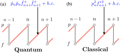
Figure 1: Schematic representation of linear hopping (solid gray lines) and interaction terms (red shaded lines) for the quantum Hubbard case (a) and the classical nonlinear case (b).

IV.2 Dynamics of two interacting particles

Let us propagate two interacting particles initially located at the same site – hence avoiding unpaired caged particles. Tovmasyan et al. (2018) For convenience and without much loss of generality, we consider distinguishable bosons. We compute the time-evolution of their wave-function $\ket{\Psi}$ which is governed by a two-dimensional lattice Schrödinger equation whose coordinates $(n,k)$ represent the spatial position of each boson – see Appendix B. We consider a network for $N=40$ unit cells and compute the local density $\rho_{n,k}$ of the two particles and the correspondent one-dimensional probability distribution function (PDF) of the particle density defined as $Q_{n}=\sum_{k=1}^{N}\rho_{n,k}$.

As the single particle Hamiltonian $\hat{\mathcal{H}}_{0}$ testbed, we consider the quantum version of model A Danieli et al. (2020a)

$$\hat{\mathcal{H}}_{0}=\sum_{n} \left[-2\hat{a}_{n}^{\dagger}\hat{b}_{n}+\sqrt{3}\left(\hat{a}_{n}^{\dagger}\hat{a}_{n+1}+\hat{a}_{n}^{\dagger}\hat{b}_{n+1}\right.\right.$$

$$\qquad\qquad\quad\left.\left.-\hat{b}_{n}^{\dagger}\hat{a}_{n+1}-\hat{b}_{n}^{\dagger}\hat{b}_{n+1}\right)+\text{h.c.}\right]$$ (12)

whose classical version satisfies the nonlinear caging condition $|z_{1}|^{2}=|w_{1}|^{2}$ in the presence of Kerr nonlinearity, and model B Danieli et al. (2020a)

$$\hat{\mathcal{H}}_{0}=\sum_{n} \left[\sqrt{3}\hat{a}_{n}^{\dagger}\hat{a}_{n+1}+3\hat{a}_{n}^{\dagger}\hat{b}_{n+1}\right.$$

$$\left.-\hat{a}_{n}^{\dagger}\hat{b}_{n-1}-\sqrt{3}\hat{b}_{n}^{\dagger}\hat{b}_{n+1}+\text{h.c.}\right]$$ (13)

whose classical version breaks the caging condition for the same nonlinearity. Note that both Hamiltonians are related to each other and to their fully detangled parent ABF Hamiltonian through proper LUTs. We now add the Bose-Hubbard interaction (8) to both models and evolve the two particles.

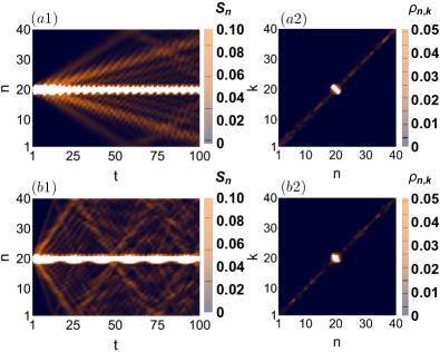
Figure 2: Model A, Eq. (12) combined with the Hubbard interaction satisfies the condition for the existence of conserved quantities. (a1) Time evolution of $Q_{n}$ and (b1) local density $\rho_{n,k}$ at time $t=100$, both for $U=1$. (a2-b2) Same as (a1-b1) but for $U=5$.

In Fig. 2 (a1-b1) we plot the time-evolution of $Q_{n}$ for model A for two interaction strengths $U=1$ (top) and $U=5$ (bottom) respectively. Both cases show that a part of the PDF is propagating ballistically - indicating the spreading of the particle pair along the network, breaking single particle caging. Simultaneously, we observe that a substantial portion of $Q_{n}$ remains localized at unit cell $n=\frac{N}{2}$ (the initial location of both particles). This is further detailed in Fig. 2 (a2-b2), where we plot the local density $\rho_{n,k}$ at time $t=100$ for $U=1$ and $U=5$ respectively. Firstly, these panels show that the delocalization and ballistic spreading of a part of the wave-function $\ket{\Psi}$ occurs along the diagonal $k=n$, which indicates that the particles have to stay bound in order to delocalize. Secondly, these plots show a large amplitude density peak at the original launching site. Such long-lasting localized excitations hint at the existence of non-propagating spatially compact states of two interacting particles which have been excited by placing both particles initially in the same cell – akin to those predicted in the AB diamond chain. Vidal et al. (2000)

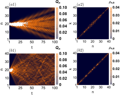
Figure 3: Model B, Eq. (12), combined with the Hubbard interaction does not possess conserved quantities. (a1) Time evolution of $Q_{n}$ and (b1) local density $\rho_{n,k}$ at time $t=100$, both for $U=1$. (a2-b2) Same as (a1-b1) but for $U=5$.

As expected, the signatures of caged states are completely absent for model B that does not obey the fine-tuning condition. Indeed, in Fig. 3 (a1-b1) we show the time-evolution of $Q_{n}$ for $U=1$ (top) and $U=5$ (bottom) respectively. These plots again show ballistic spreading, i.e. the existence of spatially extended bound states. However, no considerable localized fraction of the PDF $Q_{n}$ is observed. This is also confirmed in Fig. 3 (a2-b2), where the the local density $\rho_{n,k}$ at time $t=100$ is shown for $U=1$ and $U=5$ respectively.

IV.3 Interaction renormalized compact states

To explain and generalize the results in Fig. 2 for model A, we consider a finite number $M$ of interacting indistinguishable bosons. The wave function $\ket{\psi}$ of $M$ interacting particles can be expanded in a Fock states basis of $M$ particles as $\ket{\psi}=\sum_{{\mathbf{n}}}\varphi_{\mathbf{n}}\cdot\ket{v_{\mathbf{n}}}_{\bf a,b}$ – see Appendix B. Its time evolution is governed by the M-dimensional lattice Schrödinger equation

$$i\dot{\varphi}_{\mathbf{n}}=\left[A+UV_{M}\right]\varphi_{\mathbf{n}}+\sum_{j=1}^{M}\left[T_{j}\varphi_{{\mathbf{n}}+{\mathbf{e}}_{j}}+T_{j}^{\dagger}\varphi_{{\mathbf{n}}-{\mathbf{e}}_{j}}\right].$$ (14)

Here $\varphi_{\mathbf{n}}$ is a complex vector with $2^{M}$ components, while $A$ and $\{T_{j}\}_{j\leq M}$ are square matrices describing the dynamics of the noninteracting particles. The diagonal matrix $V_{M}$ encodes the interaction between particles described by the Hamiltonian $\hat{\mathcal{H}}_{1}$ (8).

The Hamiltonian $\hat{\mathcal{H}}_{0}$ describes $M$ non-interacting particles and can be fully detangled via a sequence of unitary transformations. Danieli et al. (2020a) Likewise, the $M$-dimensional Schrödinger system Eq. (14) for $U=0$ has only flatbands, and it can be mapped to a fully disconnected network (Appendix B.4). We now apply the detangling procedure to Eq. (14) in the presence of the interaction $U\neq 0$. The matrix $V_{M}$ induces a coupling network between the detangled sites which describes dispersive states of interacting particles and – under the fine-tuning condition $|z_{1}|^{2}=|w_{1}|^{2}$ highlighted in Ref. Danieli et al., 2020a – renormalized compact states of interacting particles. We will first consider $M=2$ and apply induction for $3\leq M$.

IV.3.1 Two particles

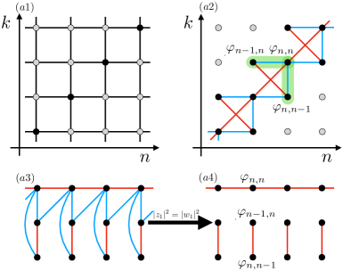
Figure 4: (a1) 2D network in Eq. (14) for $M=2$ particles. Each dot indicates one unit cell $\varphi_{n,k}$, and the black lines represent the hopping between cells. The black dots indicate the main diagonal $k=n$ where interaction applies. (a2) Rotated network. (a3) Unfolding into a 1D chain in Eq. (15) along the main diagonals of the rotated 2D network in (a2). (a4) Same as (a3) for $|z_{1}|^{2}=|w_{1}|^{2}$. The blue links in (a3) disappeared leaving components detangled from the dispersive chain and representing the renormalized compact states.

For $M=2$ interacting particles, Eq. (14) reduces to a two dimensional network – shown in Fig. 4(a1). In the noninteracting case, this network has four flatbands at $E=\pm 2$ and $E=0$ (doubly degenerate) and it can be mapped to a fully disconnected 2D lattice. In this new representation, the interaction matrix $V_{2}$ induces a coupled network along the diagonals $k=n,n\pm 1$ of Eq. (14), governed by the equation

$$i\dot{\eta}_{n}=K_{D}\eta_{n}+H_{D}\eta_{n+1}+H_{D}^{\dagger}\eta_{n+1}$$ (15)

for the unit cell $\eta_{n}=(\varphi_{n-1,n},\varphi_{n,n},\varphi_{n,n-1})$ – as shown in Fig. 4(a2).

For $k\neq n,n\pm 1$ – away from the diagonal – the rotated network Eq. (14) remains fully detangled, since these sites correspond to product states of two particles caged far from each other and therefore insensitive to the Hubbard interaction. At the diagonal lines $k=n,n\pm 1$, the 1D chain Eq. (15) - highlighted in Fig. 4(a3) - yields transporting extended states representing two interacting particles coherently evolving along the system and breaking the single particle caging – as was discussed in Sec. IV.2. However, the fine-tuning $|z_{1}|^{2}=|w_{1}|^{2}$ reduces Eq. (15) to a lattice with detangled compact interacting states similar to previously reported detanglings of CLSs in the presence of other dispersive states Flach et al. (2014) (see Fig. 4(a4) and details in Appendix C.1). This implies that:

• the diagonal $k=n$ in the $\varphi_{n,n}$ coordinates yields dispersive states of two paired particles freely moving along the chain – see Ref. Tovmasyan et al., 2018 and Sec. III;

• the detangled component described by $(\varphi_{n-1,n},\varphi_{n,n-1})$ yields degenerate compact states of two interacting particles with renormalized $U$-dependent energies.

Let us compute explicitly the energies of both types of states – dispersive and compact ones – for an example of a $\nu=2$ lattice satisfying $|z_{1}|^{2}=|w_{1}|^{2}$. Without loss of generality, to simplify our analytics instead of choosing model A in Eq.(12) we present our results for a test case obtained for $z_{i}=\cos\pi/4$, $w_{i}=\sin\pi/4$ for $i=1,2$ in Eqs. (9,10). The dispersive component in $\varphi_{n,n}$ leads to a characteristic polynomial (Appendix C.2)

$$p_{D}(E,k;U) =E[E^{3}-UE^{2}-16E+8U(1-\cos k)]$$

$$\equiv E\,g_{D}(E,k;U)$$ (16)

yielding four bands: one flat at $E=0$ and three dispersive bands given by zeroes of $g_{D}(E,k;U)$. The decoupled component $(\varphi_{n-1,n},\varphi_{n,n-1})$ leads to the characteristic polynomial (Appendix C.2)

$$p_{F}(E;U) =E^{3}(E^{2}-16)(E^{3}-UE^{2}-16E+8U)$$

$$\equiv E^{3}(E^{2}-16)\cdot g_{F}(E;U)$$ (17)

yielding five non-renormalized bands at $E=0,\pm 4$ and three bands with $U$-renormalized energies as zeroes of $g_{F}(E;U)$. Notably, Eqs. (16,17) are very similar to those obtained for two interacting spinful fermions AB diamond chain Vidal et al. (2000).

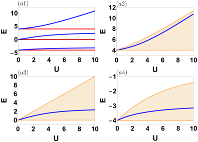
Figure 5: (a1) Non-renormalized degenerate energies (red lines) of two noninteracting CLSs and renormalized energies (blue curves) of two compactly bound interacting particles versus $U$. (a2-a4) Renormalized energies (blue curve) within the dispersive bands (orange areas) of 2IP bound states.

In Fig. 5(a1) we show the non-renormalized (red horizontal lines) and the renormalized degeneracies (blue curves) versus the interaction strength $U$. In the remaining three panels Fig. 5(a2-a4) we plot each renormalized degeneracy shown in panel (a1) and one of the three dispersive bands (orange shaded areas) obtained as zeroes of $g_{D}(E,k;U)$ in Eq. (16). We also observe that all the renormalized energies (blue curves) lie within one of the dispersive bands – as for any $U$ it holds that $g_{F}(E,U)=g_{D}(E,0;U)$ – characterizing these renormalized compact states as quantum two particles bound states in the continuum (BIC). Hsu et al. (2016)

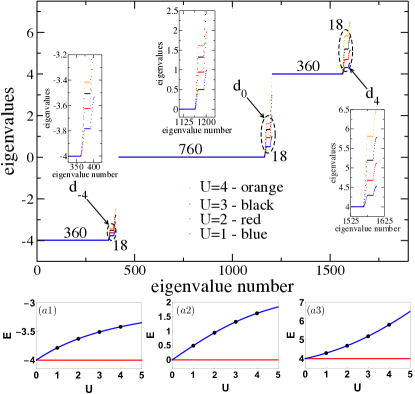
Figure 6: (main) Eigenvalues of $M=2$ interacting bosons for $N=20$. The numbers count the degenerate eigenvalues. (a1-a3) Renormalized energies (blue curves) versus $U$ and numerically obtained degeneracies (black dots) at the region $d_{-4}$ (a1), $d_{0}$ (a2), and $d_{4}$ (a3).

We tested these results numerically by diagonalizing the two dimensional network given by Eq. (14) for $M=2$ bosons at $U=1,2,3,4$ and $N=20$ unit cells. The results are reported in the upper plot of Fig. 6. We found the expected non-renormalized degeneracies at $E=0,\pm 4$ and three renormalized degeneracies labeled $d_{0},d_{\pm 4}$. The extracted degeneracy values in each region are shown with black dots in Fig. 6(a1-a3) for $U=1,2,3,4$. The comparison with the analytical (blue) curves reported in Fig. 5 shows excellent agreement. Moreover, as indicated by the numbers in the main plot of Fig. 6, the non-renormalized degeneracies at $E=0,\pm 4$ scale as $N^{2}$ while the renormalized energies scale as $N$, indicating that the renormalized compact states have macroscopic degeneracy.

These energy-renormalized states are beyond the grasp of the conserved quantities in Ref. Tovmasyan et al., 2018 and Sec. III and they result in exact two particle quantum caging. Such exact caging manifests in e.g. beating of spatially compact excitations between non-renormalized and renormalized two particles states – as shown in Fig. 7. Numerically we compute the local density $\rho_{n,k}$ of the two particles and the corresponding one-dimensional PDF of the particle density $Q_{n}$ for $U=1$ (a1) and $U=2$ (a2). As initial condition we take $E=0$ caged states of two non-interacting particles. In both panels of Fig. 7, we observe that the oscillation period $P$ (main plots; horizontal white measuring arrow) is related to the energy difference $\Delta$ (insets; vertical black measuring arrow) between renormalized and non-renormalized energies of caged states as $\Delta\approx\frac{2\pi}{P}$.

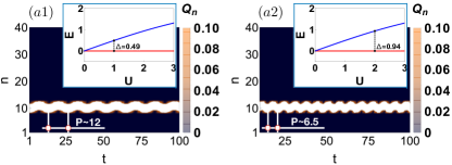
Figure 7: Time evolution of $Q_{n}$ for $U=1$ (a) and $U=2$ (b) with oscillation period $P$. Insets: zoom of Fig.5(a1) and energy difference $\Delta$. The initial conditions are $E=0$ caged states of two non-interacting particles.

IV.3.2 Three particles and beyond

The renormalized compact states of $M=2$ particles existing for Hamiltonian $\hat{\mathcal{H}}$ in Eq. (7,8) under the condition $|z_{1}|^{2}=|w_{1}|^{2}$ constitute the base case to show inductively the existence of such states for any finite number $3\leq M<\infty$ of interacting particles on an infinite lattice $N\rightarrow\infty$. The induction scheme unfolds as follows:

1. The interaction matrix $V_{M}$ in Eq. (14) can be written as a sum of $M$ matrixes

   $$V_{M}=\sum_{j=1}^{M}V_{M,n_{j}}.$$ (18)

   Each $V_{M,n_{j}}$ describes the interaction between $M-1$ particles, and it is obtained from $V_{M}$ by taking the $j^{th}$ particle as free (Appendix D.1). For any $1\leq j\leq M$, each interaction matrix $V_{M,n_{j}}$ acts on the $M-1$-dimensional networks obtained by fixing $n_{j}=const$ in the $M$-dimensional network Eq. (14);

2. Inductive hypothesis: in each $M-1$-dimensional networks, the matrix $V_{M,n_{j}}$ yields renormalized compact states of $M-1$ interacting particles. These states lie in components detangled from dispersive chains representing transporting states of paired particles - see Ref. Tovmasyan et al., 2018 and Sec. III;

3. At the main diagonal of Eq. (14), the detangled components encoding the renormalized compact states of $M-1$-particles merge, forming a larger detangled component. The $M-1$-particles compact states combine and yield compact states of $M$ particles whose energy is further renormalized.

Let us visualize this inductive step for $M=3$ particles. In this case, Eq. (14) becomes a three dimensional network which can be fully detangled via a finite sequence of unitary transformations for $U=0$. Following Eq. (18), the interaction matrix $V_{3}$ in Eq. (14) can be decomposed as

$$V_{3} =V_{3,n}+V_{3,k}+V_{3,s}$$ (19)

Each matrix $V_{3,n},V_{3,k},V_{3,s}$ in Eq. (19) is reported in Appendix D.2 and is obtained from $V_{3}$ by considering one noninteracting particle and two interacting ones. Each matrix $V_{3,n},V_{3,k},V_{3,s}$ applies to a 2D network manifold (plane) of Eq. (14) obtained for $n=n_{0}$, $k=k_{0}$, and $s=s_{0}$ respectively – as shown in Fig. 8(a1-a3).

We consider each matrix in Eq. (19) separately, starting with $V_{3,n}$. In this case, along the diagonal $k=s$ of each plane $n=n_{0}$, the matrix $V_{3,n}$ induces a one-dimensional chain Eq. (15). For the fine-tuned Hamiltonian $\hat{\mathcal{H}}$ with $|z_{1}|^{2}=|w_{1}|^{2}$ in Eq. (7,8), the one-dimensional chain Eq. (15) decouples into a dispersive part with additional detangled components – as shown in Fig. 8(b1). Identical outcomes follow considering $V_{3,k}$ and $V_{3,s}$ – as shown in Fig. 8(b2,b3). Indeed, along the diagonals $s=n$ ($s=k$) in each plane $k=k_{0}$ ($s=s_{0}$), the matrix $V_{3,k}$ ($V_{3,s}$) induces one-dimensional chains Eq. (15) which decouple for the fine-tuned Hamiltonian $\hat{\mathcal{H}}$.

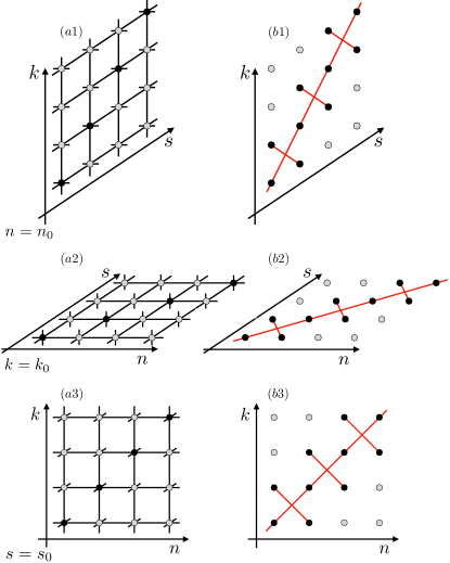
Figure 8: The graphical illustration of the decomposition given by Eq. (19). (a1) plane for $n=n_{0}$ of the 3D network Eq. (14) defined with $V_{3,n}$. Each dot indicates one unit cell $\varphi_{n,k,s}$, and the black lines are the hopping between cells. The black dots indicate the diagonal $k=s$ where $V_{3,n}$ applies (black dots). (b1) Rotated plane for $U\neq 0$ assuming $|z_{1}|^{2}=|w_{1}|^{2}$. (a2-b2) and (a3-b3) are the same as (a1-b1) but for $k=k_{0}$ and $s=s_{0}$ respectively.

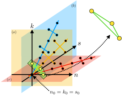
Figure 9: Diagonal structures of the rotated 3D network given by Eq. (14) for $M=3$ particles defined with the interaction matrix $V_{3}$. The detangled component with the compact states of three interacting particles is indicated with yellow dots and light green lines (also in the right top corner).

Since Eq. (14) is linear, the resulting network induced by $V_{3}$ is obtained by combining the networks induced by $V_{3,n},V_{3,k},V_{3,s}$ respectively – shown in Fig. 8(b1-b3). The result is presented in Fig. 9. In each plane $n=n_{0}$ [blue(b)], $k=k_{0}$ [red(r)], $s=s_{0}$ [orange(o)] the one-dimensional detangled chain Eq. (15) along the respective diagonal is shown. Away from the main diagonal $n_{0}=k_{0}=s_{0}$ of Eq. (14), the obtained dispersive chains yield extended transporting bound states corresponding to paired particles freely evolving along the chain, with the third unpaired particle remaining caged - as predicted in Ref. Tovmasyan et al., 2018. The detangled components within each plane represent compact states of two interacting particles with the third particle caged away from the bound pair - dubbed ”2IP+1” states. At the main diagonal $n_{0}=k_{0}=s_{0}$ of Eq. (14), the detangled components of each plane form a unique component – highlighted as yellow dots and light green lines and zoomed in the right top corner of Fig. 9. This triangular component is detangled from the dispersive chains of each plane, and it encodes compact states of three interacting particles – states dubbed ”3IP states”.

To verify these general results for Hamiltonian system $\hat{\mathcal{H}}$ fine-tuned as $|z_{1}|^{2}=|w_{1}|^{2}$ in Eq. (7,8), we studied both the detangled components representing the 2IP+1 and the 3IP compact states for our test case. We found six renormalized energies of the 2IP+1 states as zeroes of $g_{F,2+1}(E;U)$ in the polynomial

$$p_{F,2+1} (E;U)=(E^{2}-36)(E^{2}-4)^{4}$$

$$\left[E^{3}-E^{2}(U+6)+4E(U-1)+4(U+6)\right]$$

$$\left[E^{3}-E^{2}(U-6)-4E(U+1)+4(U-6)\right]$$

$$\equiv(E^{2}-36)(E^{2}-4)^{4}g_{F,2+1}(E;U)$$ (20)

which also accounts for 10 non-renormalized degeneracies at $E=\pm 2,\pm 6$. We then found twelve renormalized energies of the 3IP states as zeroes of $g_{F,3}(E;U)$ in the polynomial

$$p_{F,3} (E;U)=(E^{2}-36)(E^{2}-4)^{5}$$

$$\left[(E^{2}-36)^{2}(E^{2}-4)^{4}\right.$$

$$\left.\ -4UE(E^{2}-36)(E^{2}-28)(E^{2}-4)^{3}\right.$$

$$\left.\ +U^{2}(E^{2}-4)^{2}(6E^{6}-345E^{4}+4888E^{2}-1872)\right.$$

$$\left.\ -2U^{3}E(E^{2}-4)(2E^{6}-105E^{4}+1376E^{2}-1392)\right.$$

$$\left.\ +U^{4}(E^{8}-49E^{6}+616E^{4}-1168E^{2}+576)\right]$$

$$\equiv(E^{2}-36)(E^{2}-4)^{5}g_{F,3}(E;U)$$ (21)

which also accounts for 24 non-renormalized degeneracies at $E=\pm 2,\pm 6$. These renormalized energies are shown with blue curves in Fig. 10(a1) and (a2) respectively. In the other six panels Fig. 10(a2-a8), we plot each renormalized degeneracy of 2IP+1 states shown in panel (a1) in blue color, the renormalized degeneracy of 3IP states shown in panel (a2) in red color, and one of the six dispersive bands with orange shaded areas – the latter ones obtained as zeroes of $g_{D,2+1}$ in the polynomial

$$p_{D,2+1} (E,k;U)=(-4+E^{2})$$

$$\left[(E^{2}-36)(E^{2}-4)^{2}-2E(E^{4}-32E^{2}+112)U\right.$$

$$\left.+(E^{4}-24E^{2}+48)U^{2}+32U^{2}\cos k\right.$$

$$\left.-16(E^{2}-4)(E-U)U\cos k\right]$$

$$\equiv(-4+E^{2})g_{D,2+1}(E,k;U)$$ (22)

We observe that, as in the two particles case, all the renormalized energies lie within one dispersive bands, characterizing these renormalized compact states as quantum three particle bound states in the continuum (BIC). Hsu et al. (2016) 

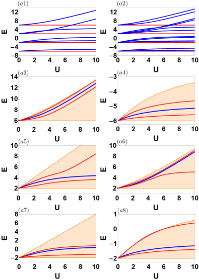
Figure 10: (a1) Non-renormalized degenerate energies (red) and renormalized energies (blue) of 2IP+1 states versus $U$. (a2) Same as (a1) for 3IP states. (a3-a8) Renormalized energies of 2IP+1 states (blue curve) and 3IP states (red curves) within the dispersive bands (orange areas) of 2IP states.

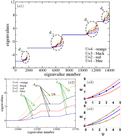
Figure 11: (a1) Eigenvalues of $M=3$ interacting bosons for $N=12$. (a2) Zoom on $d_{6}$. The numbers indicate the degeneracies of eigenvalues. (a3-a4) Renormalized energies of 2IP+1 states (blue curve) and 3IP states (red curves) versus $U$ and numerically obtained degeneracies - black dots (a3) and green dots (a4) respectively.

Similarly to the two particles states, we numerically tested these results by diagonalizing the three dimensional network Eq. (14) associated to $M=3$ bosons for $U=1,2,3,4$ and $N=12$ unit cells. The results are reported in Fig. 11. We found the expected non-renormalized degeneracies at $E=\pm 2,\pm 6$ and four renormalized degeneracies labeled $d_{\pm 2},d_{\pm 6}$. Let us focus on one of the four regions, e.g. $d_{6}$, zoomed in panel (a2). For each $U$, we observed three different degeneracies: one indicated with black arrows, and two indicated with green arrows. As shown in panel (a3), the former degeneracies (black arrows) show excellent agreement with the analytical curve reported in Fig. 5(a1) for 2IP+1 compact states. In this case, the degeneracy level is proportional to $2N^{2}$, which follows from the fact that while 2IP have degeneracy N, the additional caged single particle can be placed in $\sim 2N$ sites. As shown in panel (a4), the latter degeneracies (green arrows) show excellent agreement with the analytical curve reported in Fig. 10(a2) for 3IP compact states. In this case, the degeneracy level is proportional to $2N$ sites, indicating that also the renormalized 3IP compact states have macroscopic degeneracy.

As an inductive conjecture, this scheme can be repeated for any finite number $4\leq M<\infty$ of interacting particles by splitting the matrix $V_{M}$ split as sum of $M$ separate matrices as in Eq. (18). For e.g. $M=4$ particles, there exist: (i) renormalized compact states of three interacting particles plus one caged away (3IP+1 states); (ii) renormalized compact states made by two separate clusters of two interacting particles (2IP+2IP states); (iii) renormalized compact states of four interacting particles (4IP states). This indicates that generically for $M$ particles there exist not only degenerate interaction renormalized compact states of $M$ interacting particles, but also renormalized compact states of $M$ particles formed as product states of renormalized compact states of $L\leq M$ particles.

V Conclusions and perspectives

In this work we showed that the quantum version of classical nonlinear models exhibiting caging discussed in Ref. Danieli et al., 2020a necessarily feature an extended set of conserved quantities – number parity operators, firstly introduced in Tovmasyan et al. (2018) for specific ABF geometries – and transport is realized through moving pairs of interacting particles while single unpaired particles remain caged. We then demonstrated that the picture is more complex, as using $\nu=2$ ABF chain as testbeds we additionally showed the presence of energy renormalised multiparticle caged states – states first observed for two fermions in AB diamond chain. Vidal et al. (2000) We explicitly showed the existence of these macroscopically degenerate energy renormalized compact states for $M=2,3$ particles, and used an inductive conjecture to generalize them to any finite number $M<\infty$ of particles on an infinite lattice $N\rightarrow\infty$. Consequently, these caged many-body states generalize the extensively studied and experimentally observed single particles compact localized states Derzhko et al. (2015); Leykam et al. (2018); Leykam and Flach (2018) and hits towards quantum caging phenomena in interacting systems - see e.g. Ref. Di Liberto et al., 2019 for the AB diamond chain. Moreover, we showed that few particle $M=2,3$ caged states are bound states in the continuum (BIC) Hsu et al. (2016) – as their renormalized energies reside within dispersive bands of delocalized states of pairs of particles. Conjecturing this for any finite number of particles $M$ yields that these systems constitute a potential platform for the experimental realization of BICs in quantum systems – as discussed in Ref. Hsu et al., 2016.

The quantum caging of interacting particles highlights the all bands flat networks as a promising platform for novel phenomena in quantum many-body physics. We conjecture that these energy renormalised multiparticle caged states appear in any network whose classical version exhibits nonlinear caging. Confirmation of that hypothesis would lead to a systematic generalization of the quantum caging phenomenon in all band flat models to any number of bands $\nu\geq 3$ and higher spatial dimensions $d=2,3$. An important front is the fate of these states at the finite-density limit and their impact on the many-body dynamics. While the interaction in general allows paired particles to freely move along the system Tovmasyan et al. (2018) forbidding MBL - a fact which can be overcome by fine-tuning the interaction Danieli et al. (2020b); Kuno et al. (2020); Orito et al. (2020) – these states may contribute to anomalous thermalization phenomena. Thus the quest to search for anomalous many-body dynamics can not only be extended to interacting ABF lattices including disorder, dissipation and external fields, but also to lattice Hamiltonian supporting both flat and dispersive bands. Tilleke et al. (2020)

VI Acknowledgments

The authors thank Ihor Vakulchyk, Ajith Ramachandran, Arindam Mallick and Tilen Čadez for helpful discussions. This work was supported by the Institute for Basic Science, Korea (IBS-R024-D1).

Appendix A Rotating the quantum interaction Hamiltonian $\hat{\mathcal{H}}_{1}$

The Hubbard interaction Hamiltonian $\hat{\mathcal{H}}_{1}$ in Eq. (8) for $\nu=2$ reads

$$\hat{\mathcal{H}}_{1} =\frac{U}{2}\sum_{n\in\mathbb{Z}}\left[\hat{a}_{n}^{\dagger}\hat{a}_{n}^{\dagger}\hat{a}_{n}\hat{a}_{n}+\hat{b}_{n}^{\dagger}\hat{b}_{n}^{\dagger}\hat{b}_{n}\hat{b}_{n}\right].$$ (23)

The unitary transformation that transforms the two band ladder Eqs. (9,10) into decoupled dimers written for the operators $\hat{a}_{n},\hat{b}_{n}$ and $\hat{p}_{n},\hat{f}_{n}$ reads

$$\begin{cases}\hat{a}_{n}=e^{i\theta_{1}}\left(z_{1}\hat{p}_{n}+w_{1}\hat{f}_{n}\right)\\ \hat{b}_{n}=e^{i\theta_{1}}\left(-w_{1}^{*}\hat{p}_{n}+z_{1}^{*}\hat{f}_{n}\right)\\ \end{cases}$$ (24)

Then, $\hat{\mathcal{H}}_{1}$ in Eq. (23) turns to

$$\hat{\mathcal{H}}_{1} =\frac{U}{2}\sum_{n}\left\{(|z_{1}|^{4}+|w_{1}|^{4})\hat{p}_{n}^{\dagger}\hat{p}_{n}^{\dagger}\hat{p}_{n}\hat{p}_{n}\right.$$

$$\left.\qquad+2z_{1}^{*}w_{1}(|z_{1}|^{2}-|w_{1}|^{2})\hat{p}_{n}^{\dagger}\hat{p}_{n}^{\dagger}\hat{p}_{n}\hat{f}_{n}\right.$$

$$\left.\qquad+2z_{1}^{*2}w_{1}^{2}\hat{p}_{n}^{\dagger}\hat{p}_{n}^{\dagger}\hat{f}_{n}\hat{f}_{n}\right.$$

$$\left.\qquad+2z_{1}w_{1}^{*}(|z_{1}|^{2}-|w_{1}|^{2})\hat{p}_{n}^{\dagger}\hat{f}_{n}^{\dagger}\hat{p}_{n}\hat{p}_{n}\right.$$ (25)

$$\left.\qquad+8|z_{1}|^{2}|w_{1}|^{2}\hat{p}_{n}^{\dagger}\hat{f}_{n}^{\dagger}\hat{p}_{n}\hat{f}_{n}\right.$$

$$\left.\qquad+2z_{1}^{*}w_{1}(|w_{1}|^{2}-|z_{1}|^{2})\hat{p}_{n}^{\dagger}\hat{f}_{n}^{\dagger}\hat{f}_{n}\hat{f}_{n}\right.$$

$$\left.\qquad+2z_{1}^{2}w_{1}^{*2}\hat{f}_{n}^{\dagger}\hat{f}_{n}^{\dagger}\hat{p}_{n}\hat{p}_{n}\right.$$

$$\left.\qquad+2z_{1}w_{1}^{*}(|w_{1}|^{2}-|z_{1}|^{2})\hat{f}_{n}^{\dagger}\hat{f}_{n}^{\dagger}\hat{p}_{n}\hat{f}_{n}\right.$$

$$\left.\qquad+(|z_{1}|^{4}+|w_{1}|^{4})\hat{f}_{n}^{\dagger}\hat{f}_{n}^{\dagger}\hat{f}_{n}\hat{f}_{n}\right\}$$

The fine-tuning $|w_{1}|^{2}=|z_{1}|^{2}$ simplifies Eq. (25) to

$$\hat{\mathcal{H}}_{1} =U\sum_{n}\left\{|z_{1}|^{4}\left[\hat{p}_{n}^{\dagger}\hat{p}_{n}^{\dagger}\hat{p}_{n}\hat{p}_{n}+\hat{f}_{n}^{\dagger}\hat{f}_{n}^{\dagger}\hat{f}_{n}\hat{f}_{n}+4\hat{p}_{n}^{\dagger}\hat{f}_{n+1}^{\dagger}\hat{p}_{n}\hat{f}_{n+1}\right]\right.$$

$$\left.\quad+z_{1}^{*2}w_{1}^{2}\hat{p}_{n}^{\dagger}\hat{p}_{n}^{\dagger}\hat{f}_{n+1}\hat{f}_{n+1}+z_{1}^{*}w_{1}^{*2}\hat{p}_{n}\hat{p}_{n}\hat{f}_{n+1}^{\dagger}\hat{f}_{n+1}^{\dagger}\right\}$$ (26)

Appendix B $M$ interacting particles

B.1 Mapping an $M$-particles problem to an $M$-dimensional Schrödinger system

Let us consider the wave function $\ket{\psi}$ of $M$ interacting particles evolving on the ABF network described by the Hamiltonian $\hat{\mathcal{H}}=\hat{\mathcal{H}}_{0}+\hat{\mathcal{H}}_{1}$ in Eqs. (7,8). Then, we consider the multi-index ${\mathbf{n}}=(n_{1},\dots,n_{M})$, and the entry $n_{s}$ indicates the unit cell where where the $s^{th}$ particles is located – either on the $a$ or the $b$ chain. Hence, for a given multi-index ${\mathbf{n}}\in\mathbb{Z}^{M}$ there exist a $2^{M}$-dimensional vector of elements of the Fock basis $\ket{v_{\mathbf{n}}}_{\bf a,b}=\{\ket{v_{\mathbf{n}}^{s}}_{\bf a,b}\}_{s\leq 2^{M}}$, representing all possible particles configurations.

The wave function $\ket{\psi}$ is expanded as

$$\ket{\psi}=\sum_{{\mathbf{n}}\in\mathbb{Z}^{M}}\varphi_{\mathbf{n}}\cdot\ket{v_{\mathbf{n}}}_{\bf a,b}$$ (27)

for $\varphi_{\mathbf{n}}$ a $2^{M}$-dimensional complex vector.

Then, proceed as follows:

1. substitute Eq. (27) in the equation $i\partial_{t}\ket{\psi}=\hat{\mathcal{H}}\ket{\psi}$ with $\hat{\mathcal{H}}=\hat{\mathcal{H}}_{0}+\hat{\mathcal{H}}_{1}$ in Eqs. (7,8);

2. unfold the products in the r.h.s. of $i\partial_{t}\ket{\psi}=\hat{\mathcal{H}}\ket{\psi}$. Then regroup those terms with common index $n_{s}$ and common element of the basis $\ket{v_{\mathbf{n}}^{s}}_{\bf a,b}$

3. multiply the obtained equation by ${{}_{\bf a,b}}\langle v_{\mathbf{n}}^{s}|$. This yields the equation correspondent to the $s^{th}$ component of the vector $\varphi_{\mathbf{n}}$

4. group these equations in vector frm for $\varphi_{\mathbf{n}}$.

This results in the $M$-dimensional Schrödinger system

$$i\dot{\varphi}_{\mathbf{n}}=\left[A+UV_{M}\right]\varphi_{\mathbf{n}}+\sum_{j=1}^{M}\left[T_{j}\varphi_{{\mathbf{n}}+{\mathbf{e}}_{j}}+T_{j}^{\dagger}\varphi_{{\mathbf{n}}-{\mathbf{e}}_{j}}\right]$$ (28)

where ${\mathbf{e}}_{j}$ are the canonical basis of $\mathbb{Z}^{M}$. The matrices $A,\{T_{j}\}_{j\leq M}$ describe the lattice geometry induced by $\hat{\mathcal{H}}_{0}$, while $V_{M}$ is a diagonal matrix encapsulating the interaction $\hat{\mathcal{H}}_{1}$ whose entrees $v_{s}$ correspond to the $s^{th}$ element $\ket{v_{\mathbf{n}}^{s}}_{\bf a,b}$ of the chosen Fock basis in Eq. (27)

$$v_{s}={{}_{\bf a,b}}\bra{v_{\mathbf{n}}^{s}}\hat{\mathcal{H}}_{1}\ket{v_{\mathbf{n}}^{s}}_{\bf a,b}$$ (29)

For $U=0$ and any number of particles $M$, Eq. (28) has $2^{M}$ flatbands.

B.2 Two Interacting Particles Case

For $M=2$, Eq. (28) reduces to a two dimensional system of Schrödinger equations

$$i\dot{\varphi}_{n,k}=\left[A+UV_{2}\right]\varphi_{n,k} +T_{n}\varphi_{n+1,k}+T_{n}^{\dagger}\varphi_{n-1,k}$$

$$+T_{k}\varphi_{n,k+1}+T_{k}^{\dagger}\varphi_{n,k-1}$$ (30)

with $\varphi_{n,k}=(X_{n,k},Y_{n,k},W_{n,k},Z_{n,k})^{T}$. The onsite matrixes $A$ is

$$A =2\Gamma_{0}\begin{pmatrix}|z_{1}|^{2}-|w_{1}|^{2}&-z_{1}w_{1}&-z_{1}w_{1}&0\\ -z_{1}^{*}w_{1}^{*}&0&0&-z_{1}w_{1}\\ -z_{1}^{*}w_{1}^{*}&0&0&-z_{1}w_{1}\\ 0&-z_{1}^{*}w_{1}^{*}&-z_{1}^{*}w_{1}^{*}&|w_{1}|^{2}-|z_{1}|^{2}\\ \end{pmatrix}$$ (31)

while the hopping matrixes $T_{n},T_{k}$ are

$$T_{n} =\Gamma_{1}\begin{pmatrix}z_{1}w_{1}^{*}&0&z_{1}^{2}&0\\ 0&z_{1}w_{1}^{*}&0&z_{1}^{2}\\ -(w_{1}^{*})^{2}&0&-z_{1}w_{1}^{*}&0\\ 0&-(w_{1}^{*})^{2}&0&-z_{1}w_{1}^{*}\\ \end{pmatrix}$$ (32)

$$T_{k} =\Gamma_{1}\begin{pmatrix}z_{1}w_{1}^{*}&z_{1}^{2}&0&0\\ -(w_{1}^{*})^{2}&-z_{1}w_{1}^{*}&0&0\\ 0&0&z_{1}w_{1}^{*}&z_{1}^{2}\\ 0&0&-(w_{1}^{*})^{2}&-z_{1}w_{1}^{*}\\ \end{pmatrix}$$ (33)

for $\Gamma_{0}=|w_{2}|^{2}-|z_{2}|^{2}$ and $\Gamma_{1}=2z_{2}w_{2}$. The matrix $V_{2}$ encoding the interaction reads

$$V_{2} =\begin{pmatrix}\delta_{n,k}&0&0&0\\ 0&0&0&0\\ 0&0&0&0\\ 0&0&0&\delta_{n,k}\\ \end{pmatrix}.$$ (34)

For $U=0$, Eq. (30) has four flatbands: one at energy $E=2$ and one $E=-2$; and two at $E=0$.

B.3 Three Interacting Particles Case

For $M=3$, Eq. (28) reduces to a three dimensional system of Schrödinger equations

$$i\dot{\varphi}_{n,k,s}=\left[A+UV_{3}\right]\varphi_{n,k,s} +T_{n}\varphi_{n+1,k,s}+T_{n}^{\dagger}\varphi_{n-1,k,s}$$

$$+T_{k}\varphi_{n,k+1,s}+T_{k}^{\dagger}\varphi_{n,k-1,s}$$

$$+T_{s}\varphi_{n,k,s+1}+T_{s}^{\dagger}\varphi_{n,k,s-1}.$$ (35)

for the eight-component vector

$$\varphi_{n,k,s}=( X_{n,k,s},Y^{(1)}_{n,k,s},Y^{(2)}_{n,k,s},W^{(3)}_{n,k,s},$$

$$W^{(1)}_{n,k,s},W^{(2)}_{n,k,s},W^{(3)}_{n,k,s},Z_{n,k,s})^{T}.$$ (36)

We skip the cumbersome matrixes $A,T_{n},T_{k},T_{s}$, and only report the matrix $V_{3}$ encoding the interaction

$$V_{3} =\footnotesize\begin{pmatrix}\Delta_{n,k,s}&0&0&0&0&0&0&0\\ 0&\delta_{n,k}&0&0&0&0&0&0\\ 0&0&\delta_{n,s}&0&0&0&0&0\\ 0&0&0&\delta_{k,s}&0&0&0&0\\ 0&0&0&0&\delta_{k,s}&0&0&0\\ 0&0&0&0&0&\delta_{n,s}&0&0\\ 0&0&0&0&0&0&\delta_{n,k}&0\\ 0&0&0&0&0&0&0&\Delta_{n,k,s}\end{pmatrix}$$ (37)

where for $\Delta_{n,k,s}=\delta_{n,k}+\delta_{n,s}+\delta_{k,s}$. For $U=0$, Eq. (35) has eight flatbands: one at energy $E=3$ and one $E=-3$; three at $E=1$ and three at $E=-1$.

B.4 Detangling the $M$-dimensional Schrödinger system for noninteracting particles

The single particle Hamiltonian $\hat{\mathcal{H}}_{0}$ in Eq. (7) can be fully detangled via a sequence of 3 unitary transformations (two rotations and one unit-cell redefinition - Ref. Danieli et al., 2020a). As a consequence, this holds also for its associated Schrödinger system Eq. (28) for $U=0$. In this case the detangling procedure consists in a sequence of $3M$ unitary transformations, where each triplet of transformations consists in two unitary rotations and one unit cell redefinition. Each triplet of coordinate redefinitions recursively zeroes one of the hopping matrix $T_{j}$ and redefine the intra-cell matrix $A$. After $M$ triplets of unitary transformations all hopping matrixes $\{T_{j}\}_{j\leq M}$ vanish, and the matrix $A$ turn diagonal with the $2^{M}$ flatband energies as diagonal entrees.

By applying this procedure, the two dimensional system Eq. (30) is equivalent to a fully detangled network

$$i\dot{\varphi}_{n,k} =A_{6}\varphi_{n,k}\ ,\qquad A_{6}=\begin{pmatrix}-2&0&0&0\\ 0&0&0&0\\ 0&0&0&0\\ 0&0&0&2\\ \end{pmatrix}.$$ (38)

where the diagonal elements of $A_{6}$ in Eq. (38) are the flatband energies.

Likewise, the three dimensional system Eq. (35) is ultimately equivalent to a fully detangled network

$$i\dot{\varphi}_{n,k,s} =A_{9}\varphi_{n,k,s}.$$ (39)

The diagonal elements of the onsite matrix $A_{9}$ in Eq. (39) are the flatband energies.

Appendix C Renormalized compact states of two interacting particles

C.1 Lattice of Fano defects

The one-dimensional chain shown in Fig. 3(a2) along the three main diagonals $k=n,n\pm 1$ of the rotated Eq. (30)

$$i\dot{\eta}_{n}=K_{D}\eta_{n}+H_{D}\eta_{n+1}+H_{D}^{\dagger}\eta_{n+1}$$ (40)

for the unit cell $\eta_{n}=(\varphi_{n-1,n},\varphi_{n,n},\varphi_{n,n-1})$ is defined by the block matrixes $K_{D},H_{D}$ which depend on the interaction strength $U$

$$K_{D}=\begin{pmatrix}V^{(n-1,n)}&U\bar{T}_{n}^{(n-1,n)}&UB\\ U\bar{T}_{n6}^{(n-1,n)\dagger}&V^{(n,n)}&U\bar{T}_{k}^{(n,n-1)}\\ UB^{\dagger}&U\bar{T}_{k}^{(n,n-1)\dagger}&V^{(n,n-1)}\end{pmatrix},$$ (41)

$$H_{D}=U\begin{pmatrix}\mathbb{O}_{4}&\mathbb{O}_{4}&\mathbb{O}_{4}\\ \mathbb{O}_{4}&C&\bar{T}_{n}^{(n,n+1)}\\ \mathbb{O}_{4}&\mathbb{O}_{4}&\mathbb{O}_{4}\end{pmatrix}$$ (42)

We omit the cumbersome definitions of the blocks defining $K_{D},H_{D}$.

It turns out that the hopping matrix $\bar{T}_{k}^{(n,n-1)},\bar{T}_{n}^{(n-1,n)},\bar{T}_{n}^{(n,n+1)}$ have $\xi=z_{1}w_{1}^{*}(|z_{1}|^{2}-|w_{1}|^{2})$ as a common prefactor. The fine-tuning condition $|z_{1}|^{2}=|w_{1}|^{2}$ yields $\xi=0$ and the matrixes in Eqs. (41,42) reduce to

$$K_{D}=\begin{pmatrix}V^{(n-1,n)}&\mathbb{O}_{4}&UB\\ \mathbb{O}_{4}&V^{(n,n)}&\mathbb{O}_{4}\\ UB^{\dagger}&\mathbb{O}_{4}&V^{(n,n-1)}\end{pmatrix}$$ (43)

$$H_{D}=U\begin{pmatrix}\mathbb{O}_{4}&\mathbb{O}_{4}&\mathbb{O}_{4}\\ \mathbb{O}_{4}&C&\mathbb{O}_{4}\\ \mathbb{O}_{4}&\mathbb{O}_{4}&\mathbb{O}_{4}\end{pmatrix}$$ (44)

and the network in Eq. (40) reduces to a lattice of Fano-defects Flach et al. (2014): it decouples in a $4$-components dispersive chain

$$i\dot{\varphi}_{n,n}=V^{(n,n)}\varphi_{n,n}+U\left[C\varphi_{n+1,n+1}+C^{\dagger}\varphi_{n-1,n-1}\right]$$ (45)

and a detangled (Fano) part

$$i\frac{\partial}{\partial t}\begin{pmatrix}\varphi_{n-1,n}\\ \varphi_{n,n-1}\\ \end{pmatrix}=\begin{pmatrix}V^{(n-1,n)}&UB\\ UB^{\dagger}&V^{(n,n-1)}\end{pmatrix}\begin{pmatrix}\varphi_{n-1,n}\\ \varphi_{n,n-1}\\ \end{pmatrix}$$ (46)

shown in Fig. 4(b4) of the main text.

C.2 An example

In the case of the test case obtained with $z_{i}=\cos\pi/4$, $w_{i}=\sin\pi/4$ for $i=1,2$ in Eqs. (9,10), the onsite matrixes $V_{7}^{(n,n)},V_{7}^{(n-1,n)},V^{(n,n-1)}$ read

$$V^{(n,n)} =\frac{1}{4}\begin{pmatrix}U-16&0&0&U\\ 0&U&U&0\\ 0&U&U&0\\ U&0&0&U+16\\ \end{pmatrix},$$ (47)

$$V^{(n-1,n)} =\frac{1}{8}\begin{pmatrix}U-32&-U&U&-U\\ -U&U&-U&U\\ U&-U&U&-U\\ -U&U&-U&U+32\\ \end{pmatrix},$$ (48)

$$V^{(n,n-1)} =\frac{1}{8}\begin{pmatrix}U-32&U&-U&-U\\ U&U&-U&-U\\ -U&-U&U&U\\ -U&-U&U&U+32\\ \end{pmatrix},$$ (49)

while the matrixes $B,C$ read

$$B=\frac{1}{8}\begin{pmatrix}1&1&-1&-1\\ -1&-1&1&1\\ 1&1&-1&-1\\ -1&-1&1&1\end{pmatrix},\quad C=\frac{1}{8}\begin{pmatrix}1&1&1&1\\ -1&-1&-1&-1\\ -1&-1&-1&-1\\ 1&1&1&1\end{pmatrix}.$$ (50)

The dispersive component Eq. (45) has a characteristic polynomial

$$p_{D}(E,k;U) =E[E^{3}-UE^{2}-16E+8U(1-\cos k)]$$

$$\equiv E\,g_{D}(E,k;U)$$ (51)

The detangled component Eq. (46) has characteristic polynomial

$$p_{F}(E;U) =E^{3}(E^{2}-16)(E^{3}-UE^{2}-16E+8U)$$

$$\equiv E^{3}(E^{2}-16)\cdot g_{F}(E;U)$$ (52)

Appendix D Interaction matrix $V_{M}$ decomposition

D.1 Recursive formula

If from $M$ interacting particles we form $M$ groups of $M-1$ interacting particles by taking the $j^{th}$ as free, then from a state $\ket{v_{\mathbf{n}}^{s}}_{a,b}$ we get $M$ states $\ket{v_{\mathbf{n}}^{s,j}}_{a,b}$. It then follows the set of $M$ coefficients

$$v_{s}^{j}={{}_{a,b}}\bra{v_{\mathbf{n}}^{s,j}}\hat{\mathcal{H}}_{1}\ket{v_{\mathbf{n}}^{s,j}}_{a,b}$$ (53)

Let us suppose that all $M\geq 3$ particles are on chain $a$ (likewise, chain $b$). It then follows

$$v_{s}=\sum_{t=1}^{M}\sum_{r=t}^{M}\delta_{n_{t},n_{r}}\ ,\qquad v_{s}^{j}=\sum_{\begin{subarray}{c}t=1\\ t\neq j\end{subarray}}^{M}\sum_{r=t}^{M}\delta_{n_{t},n_{r}}$$ (54)

since the Kroneker delta involving $n_{j}$ are excluded (the $j^{th}$ particle is free). This yields that the sum of $v_{s}^{j}$ is

$$\sum_{j=1}^{M}v_{s}^{j}=(M-2)v_{s}.$$ (55)

since any Kroneker delta $\delta_{n_{t},n_{r}}$ in $v_{s}$ is absent in $v_{s}^{t}$ and $v_{s}^{r}$ but it exists once in all the other $M-2$ terms $v_{s}^{j}$. The same relation in Eq.(55) also hold for $L$ particles on chain $a$ and $M-L$ particles on chain $b$.

We define the matrixes $V_{M,n_{j}}$ as diagonal matrixes whose diagonal elements are the coefficients $v_{s}^{j}$ in Eq. (53) divided by $M-2$. This yields the decomposition Eq. (18) for any number of particles $M\geq 3$

$$V_{M}=\sum_{j=1}^{M}V_{M,n_{j}}$$ (56)

D.2 Three particles case

From the interaction matrix $V_{3}$ in Eq. (37), we obtain the matrix

$$V_{3,n} =\footnotesize\begin{pmatrix}\delta_{k,s}&0&0&0&0&0&0&0\\ 0&0&0&0&0&0&0&0\\ 0&0&0&0&0&0&0&0\\ 0&0&0&\delta_{k,s}&0&0&0&0\\ 0&0&0&0&\delta_{k,s}&0&0&0\\ 0&0&0&0&0&0&0&0\\ 0&0&0&0&0&0&0&0\\ 0&0&0&0&0&0&0&\delta_{k,s}\end{pmatrix}.$$ (57)

by considering the particle indexed via $n$ non-interacting with the remaining two. Likewise, the matrix

$$V_{3,k} =\footnotesize\begin{pmatrix}\delta_{n,s}&0&0&0&0&0&0&0\\ 0&0&0&0&0&0&0&0\\ 0&0&\delta_{n,s}&0&0&0&0&0\\ 0&0&0&0&0&0&0&0\\ 0&0&0&0&0&0&0&0\\ 0&0&0&0&0&\delta_{n,s}&0&0\\ 0&0&0&0&0&0&0&0\\ 0&0&0&0&0&0&0&\delta_{n,s}\end{pmatrix}.$$ (58)

is obtained by considering the particle labeled by $k$ non-interacting with the other two, while the matrix

$$V_{3,s} =\footnotesize\begin{pmatrix}\delta_{n,k}&0&0&0&0&0&0&0\\ 0&\delta_{n,k}&0&0&0&0&0&0\\ 0&0&0&0&0&0&0&0\\ 0&0&0&0&0&0&0&0\\ 0&0&0&0&0&0&0&0\\ 0&0&0&0&0&0&0&0\\ 0&0&0&0&0&0&\delta_{n,k}&0\\ 0&0&0&0&0&0&0&\delta_{n,k}\end{pmatrix}.$$ (59)

is obtained by considering the particle labeled by $s$ non-interacting with the other two. The sum of these three matrixes

$$V_{3} =V_{3,n}+V_{3,k}+V_{3,s}.$$ (60)

yields $V_{3}$ in Eq. (37) – confirming the formula Eq. (56).

References

- Anderson (1958) P. W. Anderson, “Absence of diffusion in certain random lattices,” Phys. Rev. 109, 1492–1505 (1958).
- Kramer and MacKinnon (1993) B. Kramer and A. MacKinnon, “Localization: theory and experiment,” Rep. Prog. Phys. 56, 1469–1564 (1993).
- Basko et al. (2006) D.M. Basko, I.L. Aleiner, and B.L. Altshuler, “Metal–insulator transition in a weakly interacting many-electron system with localized single-particle states,” Ann. Phys. 321, 1126 – 1205 (2006).
- Aleiner et al. (2010) I. L. Aleiner, B. L. Altshuler, and G. V. Shlyapnikov, “A finite-temperature phase transition for disordered weakly interacting bosons in one dimension,” Nat. Phys. 6, 900–904 (2010).
- Pino et al. (2016) Manuel Pino, Lev B. Ioffe, and Boris L. Altshuler, “Nonergodic metallic and insulating phases of Josephson junction chains,” PNAS 113, 536–541 (2016).
- Abanin et al. (2019) Dmitry A. Abanin, Ehud Altman, Immanuel Bloch, and Maksym Serbyn, “Colloquium: Many-body localization, thermalization, and entanglement,” Rev. Mod. Phys. 91, 021001 (2019).
- Derzhko et al. (2015) Oleg Derzhko, Johannes Richter, and Mykola Maksymenko, “Strongly correlated flat-band systems: The route from heisenberg spins to hubbard electrons,” Int. J. Mod. Phys. B 29, 1530007 (2015).
- Leykam et al. (2018) Daniel Leykam, Alexei Andreanov, and Sergej Flach, “Artificial flat band systems: from lattice models to experiments,” Adv. Phys.: X 3, 1473052 (2018).
- Leykam and Flach (2018) Daniel Leykam and Sergej Flach, “Perspective: Photonic flatbands,” APL Phot. 3, 070901 (2018).
- Mielke (1991) A Mielke, “Ferromagnetic ground states for the hubbard model on line graphs,” J Phys. A: Math. and Gen. 24, L73 (1991).
- Tasaki (1992) Hal Tasaki, “Ferromagnetism in the hubbard models with degenerate single-electron ground states,” Phys. Rev. Lett. 69, 1608–1611 (1992).
- Dias and Gouveia (2015) R. G. Dias and J. D. Gouveia, “Origami rules for the construction of localized eigenstates of the Hubbard model in decorated lattices,” Sci. Rep. 5, 16852 EP – (2015).
- Morales-Inostroza and Vicencio (2016) Luis Morales-Inostroza and Rodrigo A. Vicencio, “Simple method to construct flat-band lattices,” Phys. Rev. A 94, 043831 (2016).
- Maimaiti et al. (2017) Wulayimu Maimaiti, Alexei Andreanov, Hee Chul Park, Oleg Gendelman, and Sergej Flach, “Compact localized states and flat-band generators in one dimension,” Phys. Rev. B 95, 115135 (2017).
- Röntgen et al. (2018) M. Röntgen, C. V. Morfonios, and P. Schmelcher, “Compact localized states and flat bands from local symmetry partitioning,” Phys. Rev. B 97, 035161 (2018).
- Toikka and Andreanov (2018) L A Toikka and A Andreanov, “Necessary and sufficient conditions for flat bands in m-dimensional n-band lattices with complex-valued nearest-neighbour hopping,” J Phys. A: Math. Theor 52, 02LT04 (2018).
- Maimaiti et al. (2019) Wulayimu Maimaiti, Sergej Flach, and Alexei Andreanov, “Universal flat band generator from compact localized states,” Phys. Rev. B 99, 125129 (2019).
- Vidal et al. (1998) Julien Vidal, Rémy Mosseri, and Benoit Douçot, “Aharonov-Bohm cages in two-dimensional structures,” Phys. Rev. Lett. 81, 5888–5891 (1998).
- Douçot and Vidal (2002) Benoit Douçot and Julien Vidal, “Pairing of cooper pairs in a fully frustrated josephson-junction chain,” Phys. Rev. Lett. 88, 227005 (2002).
- Fang et al. (2012a) Kejie Fang, Zongfu Yu, and Shanhui Fan, “Photonic Aharonov-Bohm Effect Based on Dynamic Modulation,” Phys. Rev. Lett. 108, 153901 (2012a).
- Longhi (2014) Stefano Longhi, “Aharonov-Bohm photonic cages in waveguide and coupled resonator lattices by synthetic magnetic fields,” Opt. Lett. 39, 5892–5895 (2014).
- Kibis et al. (2015) O. V. Kibis, H. Sigurdsson, and I. A. Shelykh, “Aharonov-Bohm effect for excitons in a semiconductor quantum ring dressed by circularly polarized light,” Phys. Rev. B 91, 235308 (2015).
- Hasan et al. (2016) M. Hasan, I. V. Iorsh, O. V. Kibis, and I. A. Shelykh, “Optically controlled periodical chain of quantum rings,” Phys. Rev. B 93, 125401 (2016).
- Zhang and Jin (2020) S. M. Zhang and L. Jin, “Compact localized states and localization dynamics in the dice lattice,” Phys. Rev. B 102, 054301 (2020).
- Fang et al. (2012b) Kejie Fang, Zongfu Yu, and Shanhui Fan, “Realizing effective magnetic field for photons by controlling the phase of dynamic modulation,” Nature Photonics 6, 782–787 (2012b).
- Mukherjee et al. (2018) Sebabrata Mukherjee, Marco Di Liberto, Patrik Öhberg, Robert R. Thomson, and Nathan Goldman, “Experimental observation of Aharonov-Bohm cages in photonic lattices,” Phys. Rev. Lett. 121, 075502 (2018).
- Gladchenko et al. (2009) Sergey Gladchenko, David Olaya, Eva Dupont-Ferrier, Benoit Douçot, Lev B. Ioffe, and Michael E. Gershenson, “Superconducting nanocircuits for topologically protected qubits,” Nature Phys. 5, 48–53 (2009).
- Danieli et al. (2020a) Carlo Danieli, Alexei Andreanov, Thudiyangal Mithun, and Sergej Flach, “Nonlinear caging in all-bands-flat lattices,” (2020a), arXiv:2004.11871 [cond-mat.quant-gas] .
- Creutz (1999) Michael Creutz, “End states, ladder compounds, and domain-wall fermions,” Phys. Rev. Lett. 83, 2636–2639 (1999).
- Takayoshi et al. (2013) Shintaro Takayoshi, Hosho Katsura, Noriaki Watanabe, and Hideo Aoki, “Phase diagram and pair Tomonaga-Luttinger liquid in a Bose-Hubbard model with flat bands,” Phys. Rev. A 88, 063613 (2013).
- Tovmasyan et al. (2013) Murad Tovmasyan, Evert P. L. van Nieuwenburg, and Sebastian D. Huber, “Geometry-induced pair condensation,” Phys. Rev. B 88, 220510 (2013).
- Tovmasyan et al. (2016) Murad Tovmasyan, Sebastiano Peotta, Päivi Törmä, and Sebastian D. Huber, “Effective theory and emergent symmetry in the flat bands of attractive hubbard models,” Phys. Rev. B 94, 245149 (2016).
- Jünemann et al. (2017) J. Jünemann, A. Piga, S.-J. Ran, M. Lewenstein, M. Rizzi, and A. Bermudez, “Exploring interacting topological insulators with ultracold atoms: The synthetic creutz-hubbard model,” Phys. Rev. X 7, 031057 (2017).
- Tovmasyan et al. (2018) Murad Tovmasyan, Sebastiano Peotta, Long Liang, Päivi Törmä, and Sebastian D. Huber, “Preformed pairs in flat bloch bands,” Phys. Rev. B 98, 134513 (2018).
- Vidal et al. (2001) Julien Vidal, Patrick Butaud, Benoit Douçot, and Rémy Mosseri, “Disorder and interactions in Aharonov-Bohm cages,” Phys. Rev. B 64, 155306 (2001).
- Vidal et al. (2000) Julien Vidal, Benoît Douçot, Rémy Mosseri, and Patrick Butaud, “Interaction induced delocalization for two particles in a periodic potential,” Phys. Rev. Lett. 85, 3906–3909 (2000).
- Danieli et al. (2020b) Carlo Danieli, Alexei Andreanov, and Sergej Flach, “Many-body flatband localization,” Phys. Rev. B 102, 041116(R) (2020b).
- Kuno et al. (2020) Yoshihito Kuno, Takahiro Orito, and Ikuo Ichinose, “Flat-band many-body localization and ergodicity breaking in the Creutz ladder,” New J. Phys. 22, 013032 (2020).
- Orito et al. (2020) Takahiro Orito, Yoshihito Kuno, and Ikuo Ichinose, “Exact projector hamiltonian, local integrals of motion, and many-body localization with symmetry-protected topological order,” Phys. Rev. B 101, 224308 (2020).
- Flach et al. (2014) Sergej Flach, Daniel Leykam, Joshua D. Bodyfelt, Peter Matthies, and Anton S. Desyatnikov, “Detangling flat bands into Fano lattices,” Europhys. Lett. 105, 30001 (2014).
- Hsu et al. (2016) Chia Wei Hsu, Bo Zhen, A. Douglas Stone, John D. Joannopoulos, and Marin Soljacic, “Bound states in the continuum,” Nat. Rev. Mat. 1, 16048 (2016).
- Note (1) In Fig.10(a3) and (a6) one of the two 3IP renormalized energies approaches the boundary of the continuum.
- Di Liberto et al. (2019) Marco Di Liberto, Sebabrata Mukherjee, and Nathan Goldman, “Nonlinear dynamics of Aharonov-Bohm cages,” Phys. Rev. A 100, 043829 (2019).
- Tilleke et al. (2020) Simon Tilleke, Mirko Daumann, and Thomas Dahm, “Nearest neighbour particle-particle interaction in fermionic quasi one-dimensional flat band lattices,” Z. Naturforsch. A 75, 20190371 (2020).