State-of-the-art AGN SEDs for Photoionization Models: BLR Predictions Confront the Observations

Abstract

The great power offered by photoionization models of Active Galactic Nuclei (AGN) emission line regions has long been mitigated by the fact that very little is known about the spectral energy distribution (SED) between the Lyman limit, where intervening absorption becomes a problem, and  0.3 keV, where soft x-ray observations become possible. The emission lines themselves can, to some degree, be used to probe the SED, but only in the broadest terms. This paper employs a new generation of theoretical SEDs which are internally self-consistent, energy conserving, and tested against observations, to infer properties of the emission-line regions. The SEDs are given as a function of the Eddington ratio, allowing emission-line correlations to be investigated on a fundamental basis. We apply the simplest possible tests, based on the foundations of photoionization theory, to investigate the implications for the geometry of the emission-line region. The SEDs become more far-ultraviolet bright as the Eddington ratio increases, so the equivalent widths of recombination lines should also become larger, an effect which we quantify. The observed lack of correlation between Eddington ratio and equivalent width shows that the cloud covering factor must decrease as Eddington ratio increases. This would be consistent with recent models proposing that the broad-line region is a failed dusty wind off the accretion disc.

1 Introduction

It has long been the goal of AGN astrophysics to be able to use quasar emission lines to probe the centers of massive galaxies across the universe. Photoionization models are often used to do this. Reviews of such work are given in the conference volume Ferland & Savin (2001) and in the textbook Osterbrock & Ferland (2006), hereafter AGN3.

The emission lines are most sensitive to the spectral energy distribution (SED) in the unobservable FUV, EUV, and XUV regions. The interstellar medium blocks our view of this spectral region, so indirect methods must be used to predict this part of the radiation field. The emission lines also carry information about this part of the SED, and the lines can be used to constrain that region, as was done by Mathews & Ferland (1987). Most of the observed variation in emission line ratios can be characterised in a principle component analysis (Boroson & Green, 1992a). The dominant component is Eigenvector 1, which most probably represents changes in the Eddington ratio: $L/L_{\rm Edd}$ where $L$ is the bolometric luminosity and $L_{\rm Edd}$ is the Eddington luminosity, with smaller but still significant changes along Eigenvector 2, probably representing changes in mass (Boroson & Green, 1992a).

A new generation of AGN SEDs have now become available, as summarized in Done et al. (2012), Jin et al. (2012a), Jin et al. (2012b), and Jin et al. (2012c), These papers model the AGN continua from nearby, well studied objects, and stack them as a function of $L/L_{\rm Edd}$, giving a sequence of spectra which are ideal for pursuing such questions as the origin of the Eigenvector emission line sequence (Boroson & Green, 1992b; Marziani et al., 2010). The aim of this paper is to test whether the expected changes in the SEDs are consistent with the observed changes in emission line properties across this sample (see also Panda et al. (2019) for a similar study using H$\beta$ and FeII). There have been a number of studies which have tried to derive the SED directly from observations, starting with Mathews & Ferland (1987) and recently by Meléndez et al. (2011). These studies are entirely complementary to the current approach, which begins with ad initio self-consistent models of the SED. One of our goals is to propose simple but robust tests for the validity of these new models.

The optical line emission can be predicted using large photoionization codes such as Cloudy (Ferland et al., 2013). However, the differences can be illustrated more powerfully using simple first principles of photo-ionization as these give constraints simply from photon number counts. The set of SEDs used here have harder FUV spectra as $L/L_{\rm Edd}$ increases so we probe this using the broad line from He II (4686Å) as this is produced by recombination from completely ionized He, requiring photons above 52 eV. However, line equivalent widths can be affected by reddening as well as systematic uncertainties on geometry (covering factor, continuum anisotropy etc.). Hence we also compare He II with broad H$\beta$ as this is nearby at 4861Å so is similarly affected by reddening but is from hydrogen recombination so requires photons above 13.6 eV. The SEDs predict that both lines should increase in EW with $L/L_{\rm Edd}$. This is not seen in the data so it requires a systematic decrease in BLR emissivity to compensate for the predicted change, as shown in the analysis below (e.g. sec 3). The models correctly predict that the ratio of HeII/H$\beta$ should increase by a factor $\sim 2$ from the harder FUV spectrum as $L/L_{\rm Edd}$ increases from $0.1\to 1$, and by another factor of 2 for the most extreme super-Eddington Narrow Line Seyfert 1 (NLSY 1) known. The data are compatible with this, though the models form an upper envelop to the observations. Either the SED change seen in the data is not seen by the BLR (anisotropic and/or filtered emission) or the covering fraction of the high ionization lines changes by more than that of the low ionization lines.

2 Overview of the SEDs

The SEDs used here are based on the study of Jin et al. (2012c). This uses a sample of unobscured AGN with both SDSS spectra covering broad H$\beta$ and good signal-to-noise XMM-Newton UV/X-ray observations, giving a well sampled SED together with black hole mass estimator (see also Jin et al. 2012a). These 51 AGN were fit using the SED models developed by (Done et al., 2012). It has long been known that the observed broad-band SEDs of AGN are not well reproduced by a standard Shakura-Sunyaev disk with “extra” emission in the IR and X-ray (Elvis et al., 1994). The UV turns down at energies below the expected peak for a disk which extends down to the last stable circular orbit, there is an X-ray tail which extends out to high energies, and there is a soft X-ray upturn which appears to point upwards to match the UV downturn (soft X-ray excess component). Nonetheless, the optical/soft UV spectrum is generally quite well matched by the disc emission expected from a standard accretion disc.

In the standard disk models, the mass accretion rate is constant with radius, so the mass accretion rate through the outer disc sets the mass accretion rate through the entire accretion flow, irrespective of its structure. Assuming that the emissivity is standard Novikov-Thorne sets the luminosity emitted at each radius, and the full SED can then be fit assuming that this energy thermalises at large radii, but below some coronal radius, $R_{cor}$, determined by fitting the data, the energy is instead emitted as a combination of warm, optically thick Comptonisation (to fit the UV downturn and soft X-ray excess) or hot, optically thin Comptonisation (to fit the high energy X-ray tail). This gives a model which has enough components to follow the data, but with physical limitations on the energetics which allows the fits to be well constrained.

The models have undergone some development since the first study of Jin et al. (2012a). This first paper assumed that the outer disk emission thermalised to a blackbody at the effective temperature (optxagn model in xspec), whereas electron scattering within the disc atmosphere is expected to cause a shift in the observed temperature once hydrogen becomes ionised, giving a colour temperature correction (referred to as $f$) to the emission (optxagnf model in xspec: (Done et al., 2012)). This latter model is used in Jin et al. (2012c), and we base our study here on the results from this. A subsequent model upgrade which treats the soft Compton component more exactly was developed by Kubota & Done (2018), but these have yet to be fit to the data.

Jin et al. (2012c) split the sample into three sub-samples in every parameter to try to determine which was the most likely to be responsible for changes in the observed SED. To some extent, looking for a single parameter family should be doomed to failure as there is considerable spread in both mass and mass accretion rate across the sample, let alone additional scatter which could be introduced from a range in black hole spin and/or inclination angle (though hopefully the latter is small as significantly obscured objects are not included). They concluded that most of the variance was due to $L/L_{\rm Edd}$. The three SEDs resulting from the stacked low, medium and high $L/L_{\rm Edd}$ sub-samples have mean $\log L/L_{Edd}=-1.15,-0.55,-0.03$, respectively, and are show in Fig.1 normalised to the wavelength of H$\beta$. The major change in shape is the increase in disc emission in the UV, correlated with a softer X-ray tail. In the model, this implies a decreasing radius, $R_{cor}$ at which the standard disc transitions to the Comptonised components (decreasing from $155\to 60\to 13$), and to a softer spectral index of the high energy tail (photon index $\Gamma$ increasing from $1.8\to 1.9\to 2$). For comparison, the SED deduced by Mathews & Ferland (1987) is shown as the dotted line.

We extend this set of SEDs to even higher $L/L_{\rm Edd}$ by including the single object RX J0439.6-5311 (Jin et al. 2017). This is one of the most extreme Narrow Line Seyfert 1 galaxies (NLS1), and has an exquisitely well determined SED as there is very little interstellar extinction along this line of sight, so the continuum can be seen directly to 912Å in the rest frame (HST COS), and is visible again at 0.1 keV (ROSAT). Again, normalising at H$\beta$ shows that this continues the trend in SED properties, being even more dominated by the disc component, with even steeper X-ray tail. We use this set of 4 SEDs spanning nearly two orders of magnitude in $L/L_{\rm Edd}$ to calculate the expected change in H$\beta$ and He II line emission. The models clearly show differential change in the 52 eV continuum relative to the 13.6 eV continuum (marked by vertical lines) so there should also be changes in the He II and H$\beta$ line emission.

3 The “Zanstra temperature” test of recombination line equivalent widths

This section applies the test first suggested by Zanstra (1929) and described in AGN3 Section 5.10. The idea is simple. The luminosity of an H or He recombination line is proportional to the number of ionizing photons in the H or He-ionizing continuum. Each ionizing photon produces one photoionization, resulting in one recombination, so the lines count the number of photons in the FUV-EUV-XUV part of the SED. The equivalent width of an H or He recombination line is proportional to the ratio of the number of ionizing photons to the continuum under the emission line, so is a direct probe of the SED shape. While many other UV and optical lines will change too, they are far more difficult to model so are left for a later paper.

We first show the idea in terms of simple recombination theory. Detailed calculations show that each hydrogen-ionizing photon produces one hydrogen ionization (AGN3). If the central object is surrounded by clouds that are optically thick in the Lyman continuum, then the number of ionizing photons absorbed by clouds per second will be

$$N_{ion}=\frac{\Omega}{4\pi}Q(H)\ \ \ [s^{-1}]$$ (1)

where Q(H) is the total number of ionizing photons in the SED [s^-1, AGN3 Sec 2.1] and $\Omega/4\pi$ is the gas covering factor, the fraction of the ionizing photons which strike gas and are absorbed. Photoionizations and recombinations are in balance, so Equation 1 is also the number of hydrogen recombinations per second. The ratio $\alpha_{eff}(H\beta)/\alpha_{B}(H)\sim 1/8$ is the fraction of hydrogen recombinations which produce an H$\beta$ photon in Case B conditions (AGN3 Section 4.2). The number of H$\beta$ photons emitted per second is then

$$N(H\beta,Case\ B)=Q(H)\frac{\Omega}{4\pi}\frac{\alpha_{eff}(H\beta)}{\alpha_{B}(H)}\ \ \ [s^{-1}]$$ (2)

The equivalent width of the line, $EW(line)$, is then

$$EW(H\beta,Case\ B)=h\nu(H\beta)\ \lambda(H\beta)\ \frac{\Omega}{4\pi}\frac{\alpha_{eff}(H\beta)}{\alpha_{B}(H)}\frac{Q(H)}{\nu F_{\nu}(H\beta)}$$ (3)

which is approximately given by

$$EW(H\beta,Case\ B)\approx 4.81\times 10^{-13}t_{4}^{-0.06}\frac{\Omega}{4\pi}\frac{\lambda(H\beta)Q(H)}{\nu F_{\nu}(H\beta)}$$ (4)

where $t_{4}$ is the gas temperature in units of 10⁴ K and the recombination coefficients given in AGN3 are used. The equivalent equation for He II $\lambda 4686$ is

$$EW(\lambda 4686,Case\ B)\approx 9.35\times 10^{-13}t_{4}^{-0.28}\frac{\Omega}{4\pi}\frac{\lambda(4686)Q(He^{+})}{\nu F_{\nu}(\lambda 4686)}$$ (5)

In this way the equivalent width of a recombination line such as H$\beta$ or He II $\lambda 4686$ is determined by the SED and gas covering factor. This is the “Zanstra method” of determining stellar temperatures (see AGN3, Sec 5.7). Although the ideas presented here are based on foundation recombination theory, they are in accord with the BLR model predictions presented below.

The equivalent width $EW(H\beta)$ depends on the cloud covering factor $\Omega/4\pi$ since only $\Omega/4\pi$ of ionizing photons strike clouds, are absorbed, and produce an H$\beta$. If all AGN have the same $\Omega/4\pi$ then $EW(H\beta)$ directly probes the SED hardness of various objects. Alternatively, with models of the SED shape such as those described here, the equivalent width can be used to determine whether the covering factor depends on other parameters of the black hole.

Figure 1 compares the four SEDs discussed above. The photon energy is given in keV, the units used in the original SED papers, and the SEDs are normalized to have the same intensity at the wavelength of H$\beta$. This makes it simple to compare optical recombination line equivalent widths. The last term in Equation 3 is the ratio of the area in yellow in Figure 1 to the SED intensity at the wavelength of H$\beta$. The equivalent width is proportional to the number of photons continued in the yellow regions of the SEDs. The figure also marks the ionization limit for fully ionizing He, 54.4 eV. This part of the SED controls He II emission.

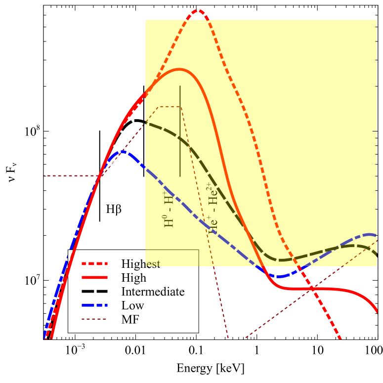
Figure 1: The four SEDs studied in this paper are compared. They are normalized to have the same intensity at the wavelength of H$\beta$, to facilitate comparison with line equivalent widths. The yellow region marks the hydrogen-ionizing part of the SED. The equivalent width of a recombination line such as H I H$\beta$ is proportional to the ionizing photon luminosity within the yellow region. The energy to fully ionize He and produce He II emission is also marked. The dotted line marked “MF” is the mean SED deduced by Mathews & Ferland (1987).

The number of ionizing photons is predicted to strongly correlate with $L/L_{\rm Edd}$. The “Highest” SED produces the most Lyman continuum photons relative to the continuum at H$\beta$ so its H$\beta$ line will also have the highest equivalent width, $\sim 1$ dex higher than the lowest Eddington ratio SED. The number of photons that can ionize helium increases even more. These considerations provide a strong, model independent, prediction that the equivalent widths of H I and He II will strongly correlate with the Eddington ratio. Although Figure 1 shows that a significant amout of energy is emitted at high energies, the tests proposed here are based on photon counting and there are relatively few high-energy photons. The SED around the ionization potentials of H and He has the most important effect on our tests.

Table 1 compares the predicted H$\beta$ and He II $\lambda 4686$ equivalent widths for the four SEDs. The rows marked “H$\beta$ Q(H)” and “He II Q(He⁺)” are straightforward applications of Equations 3 and 5 assuming Case B. This should be quite accurate for lower density gas, for instance, the NLR. The situation for H I in the BLR is more complex due to the high resulting line optical depths, Ly$\alpha$ trapping, and the importance of photoionization from excited states (Netzer, 1990) but these processes have a much smaller effect on He II since its resonance lines are destroyed by photoionization of hydrogen (Eastman & MacAlpine, 1985) with the result that He II should be closer to Case B. The rows marked “BLR” give predictions for a “standard” BLR cloud (log U =-1, log N(H) = 10) using Cloudy (Ferland et al., 2017). The H I equivalent widths are generally within $\sim 50\%$ of Case B while He II is even closer to Case B. The strong trend for increasing Eddington ratio to produce larger equivalents is obvious. The highest-Eddington-ratio objects should have recombination line equivalent widths roughly 1 dex larger than the low-Eddington-ratio objects. For reference, the ratios of changes in the ratio of number of ionizing photons for H and He and the ratio of ionizing to non-ionizing photons as a function of Eddington ratio is given by the ratios of predicted equivalent widths in this Table.

Table 1: Predicted and observed equivalent widths for H 1 $\lambda 4861$ and He II $\lambda 4686$.

$EW$(Line)	Low	Inter	High	Highest
H$\beta$ Q(H)	90.1Å	198Å	432Å	643Å
H$\beta$ BLR	128Å	268Å	527Å	828Å
H$\beta$ Obs	68 $\pm$34Å	93 $\pm$33Å	76 $\pm$39Å	25.6 $\pm$1.1Å
He II Q(He+)	26.0Å	63.0Å	181Å	492Å
He II BLR	21.2Å	50.7Å	145Å	403Å
He II Obs	12.1$\pm$9.9Å	16.4$\pm$11.2Å	10.9$\pm$8.1Å	2.1${}^{+3.6}_{-2.1}$Å
$\Omega/4\pi$(H$\beta$)	0.755$\pm 0.377$	0.470$\pm 0.167$	0.176$\pm 0.090$	0.040$\pm 0.002$
$\Omega/4\pi$(He II)	0.465$\pm$0.381	0.260$\pm$0.178	0.060$\pm$0.045	0.0043${}^{0.0073}_{0.0043}$

It is likely that clouds actually have a distribution of parameters, the Locally Optimal-Emitting Cloud (LOC) model of the emitting regions (Baldwin et al., 1995). Calculations show that the equivalent widths of the recombination lines we use here are consistent with large regions of BLR parameter space (Korista et al., 1997a) for a particular SED. Our goal here is to make differential comparisons over the range of Eddington ratio, to document the effects of changes in the SED. Whatever differences are introduced by the LOC model should not affect our differential comparison if the structure of the BLR does not change as the Eddington ratio changes. The following sections argue that large structural changes are, in fact, taking place.

4 Comparison with observations

The mean equivalent widths for the four Eddington ratio groups, as measured from the sample described by Jin et al. (2012a) and Jin et al. (2017), are listed in the “obs” rows of Table 1. The uncertainties in the first three groups represents the ensemble average while the highest $L/L_{\rm Edd}$ gives the measurement uncertainty in the single object. The equivalent widths for individual objects in the sample are shown in Figure 2, along with the mean, with different plot symbols used to indicate the sub-classes.

Two tests can be performed. The first, shown in the upper and middle panels of Figure 2, is the line equivalent width as given by Equations 3 and 5. The large stars give the predicted equivalent widths for the four groups in Table 1. These assume that clouds fully cover the continuum source, that is, $\Omega/4\pi=1$ in Equations 3 and 5. The prediction that the equivalent width should increase as the Eddington ratio increases and the SED at the ionization energies becomes harder is clear.

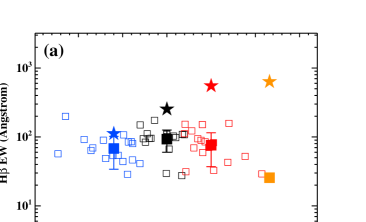
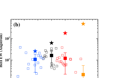
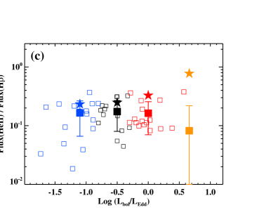
Figure 2: The H$\beta$ (top) and He II $\lambda 4686$ (middle) equivalent widths as a function of the Eddington ratio. The filled squares represent the observed values for the Eddington-ratio groups. The coloured stars give the predicted equivalent widths assuming that clouds fully cover the continuum source. Larger EW’s occur for higher Eddington ratio SEDs because of relatively more FUV flux. These predictions scale linearly with the cloud covering factor. The lower panel gives the ratio of the line equivalent widths (or fluxes), for He II / H I. This has the advantage that the cloud covering factor cancels out, and so it should have smaller cosmic scatter than the upper two panels.

The observations have a large scatter but do not follow the expected changes in equivalent width. The simple expectations of Equation 3 and 5 do not agree with observations. This could mean that the SED is incorrect, or that the cloud geometry depends on the Eddington ratio. Theory and observation can be reconciled by setting the covering factor to the ratio of the observed to theoretical equivalent widths. These required covering factors, given as the ratio of the observed equivalent width to “Q(H)” and “Q(He⁺) predictions, are given in the last two rows of Table 1.

In the next section we make a qualitative suggestion for how this might occur.

5 Discussion and conclusions

One possibility for the lack of correlation between $L/L_{\rm Edd}$ and equivalent width is that the clouds do not “see” the same SED that we do (Korista et al., 1997b). Alternatively, the geometry of the BLR could be a function of the SED, an idea that we will now discuss.

The cloud covering factor given in Table 1 decreases as the Eddington ratio increases. The consequences of changing covering factors have been discussed by, among many others, Oh et al. (2015), Lanz et al. (2019) and Lusso et al. (2013). The low Eddington ratio objects require covering factors around 50%, with the covering factor decreasing to $\sim 5\%$ for the highest Eddington ratio case. Such changes are not totally ad hoc. It has previously been suggested that an inverse correlation between covering factor and luminosity is the explanation for the “Baldwin effect”, the tendency for the UV C IV line equivalent width to decrease with increasing luminosity (Mushotzky & Ferland, 1984). X-ray observations further suggest that the covering factor varies over the range suggested by Figure 2 and becomes larger as the luminosity decreases (Ricci et al., 2013; Lawrence et al., 2013).

The ratio of the line equivalent widths, EW(He II 4686) / EW(H$\beta$), measures the number of photons with $h\nu>54$ eV relative to the number with $h\nu>13.6$ eV. This ratio has the advantage that the cloud covering factor cancels out, so it might be expected to have a smaller scatter than the equivalent widths. This ratio is shown in the lowest panel of Figure 2. Curiously, the predicted values hover over the upper envelope of the scatter. The difference in the covering factors of the H I and He II lines is within the uncertainties of the approximations made in our analysis. There is a hint of a trend in the data which parallels the theoretical expectation given in Equations 1-5. This supports the suggestion that decreasing covering factor could account for the discrepancy seen in the upper two panels. Now we consider the lower panel which traces the line ratio. The track of the predicted line ratio lies consistently above the observations, and particularly so for the highest SED. Another way of putting this is that the high-ionization lines change by more than the low ionization, requiring that their covering factor also change more.

The factor of 10 difference between the observed and theoretical H$\beta$ and He II lines strengths for the high Eddington ratio objects is a due to the change in the ionizing continuum with Eddington ratio in our adopted model. It has long been known that the ratio of the x-ray to UV is a function of luminosity (see Lusso et al. (2018) for the latest result), and a function of Eddington ratio but with very large scatter (Lusso et al., 2010). We know of no systematic study of the effects on the line spectrum of these changes in the SED. The existence of a set of comprehensive and self consistent SEDs makes this now possible. This paper is a first step in that direction.

The BLR is an optically thick structure illuminated anisotropically by the accretion disk flux. As the LOC model of the BLR shows, for a given range in number density, each emission line radiates most efficiently at a given ionising flux (e.g. Korista & Goad, 2004). The location where this (constant) flux is reached will depend on the (ionizing) luminosity (of which $L/L_{\rm Edd}$ is a good measure); it will increase with increasing luminosity (as $R\propto\sqrt{L}$). In this scenario, our observation of a decreasing BLR covering factor with increasing Eddington ratio can be explained if the BLR structure had a constant scale height. Then, as the LOC radius increases, its half-opening angle $\Phi$ (related to the covering fraction CF as $CF=sin(\Phi)$) as seen by the central AGN decreases, resulting in a reduced EW. A BLR with a constant scale height located in the equatorial plane is expected under the recent models of Czerny & Hryniewicz (2011); Czerny et al. (2017) and Baskin & Laor (2018), in which the BLR is a failed dusty wind off the accretion disk.

For the super-Eddington AGN, the change of disc structure may become important as well, which can further modulate the intensity of different emission lines. In this extreme case, the presence of a puffed up inner disk region, and/or a clumpy strong disk wind, may partially shield the ionizing flux originated from the high energy band of the SED including the soft X-ray excess and part of the UV emission. This would affect He II more than H I because the ionizing energy of He II is higher (see Figure 1), and so reduce the ratio between these two lines. This concept is discussed for super-Eddington AGN and shown as a cartoon in Jin et al. (2017).

It has become common to estimate AGN black hole masses from single-epoch spectra using the emission line luminosity as a proxy for the BLR radius instead of the optical continuum luminosity. This is because the continuum emission can suffer from contamination by the host galaxy flux in low-z sources, or by non-thermal jet emission in radio-loud sources. Our investigation predicts that for high $L/L_{\rm Edd}$ sources, the use of the line luminosity will under predict the black hole mass by factors of several because of the required changes in cloud covering factor.

Our results also suggest that changes in the SED alone are not responsible for emission line differences between NLS1, which are thought to have high Eddington ratios and so represented by our “highest” case, and broad line Seyferts. We propose that the geometry of the BLR is also likely to change.

The next step would be to study a much larger AGN sample that can be divided according to $L/L_{\rm Edd}$, black hole mass and spin.

6 Acknowledgments

GJF acknowledges support by NSF (1816537), NASA (ATP 17-ATP17-0141), and STScI (HST-AR- 15018). C.J. acknowledges the National Natural Science Foundation of China through grant 11873054, as well as the support by the Strategic Pioneer Program on Space Science, Chinese Academy of Sciences through grant XDA15052100. C.D., H.L. and M.J.W. acknowledge the Science and Technology Facilities Council (STFC) through grant ST/P000541/1 for support.

References

- Baldwin et al. (1995) Baldwin J., Ferland G., Korista K., Verner D., 1995, ApJ, 455, L119+
- Baskin & Laor (2018) Baskin A., Laor A., 2018, MNRAS, 474, 1970
- Boroson & Green (1992a) Boroson T. A., Green R. F., 1992a, ApJS, 80, 109
- Boroson & Green (1992b) Boroson T. A., Green R. F., 1992b, ApJS, 80, 109
- Czerny & Hryniewicz (2011) Czerny B., Hryniewicz K., 2011, A&A, 525, L8
- Czerny et al. (2017) Czerny B., et al., 2017, ApJ, 846, 154
- Done et al. (2012) Done C., Davis S. W., Jin C., Blaes O., Ward M., 2012, MNRAS, 420, 1848
- Eastman & MacAlpine (1985) Eastman R. G., MacAlpine G. M., 1985, ApJ, 299, 785
- Elvis et al. (1994) Elvis M., et al., 1994, ApJS, 95, 1
- Ferland & Savin (2001) Ferland G., Savin D. W., eds, 2001, Spectroscopic Challenges of Photoionized Plasmas Astronomical Society of the Pacific Conference Series Vol. 247
- Ferland et al. (2013) Ferland G. J., et al., 2013, Revista Mexicana de Astronomia y Astrofisica, 49, 137
- Ferland et al. (2017) Ferland G. J., et al., 2017, Revista Mexicana de Astronomia y Astrofisica, 53, 385
- Jin et al. (2012a) Jin C., Ward M., Done C., Gelbord J., 2012a, MNRAS, 420, 1825
- Jin et al. (2012b) Jin C., Ward M., Done C., 2012b, MNRAS, 422, 3268
- Jin et al. (2012c) Jin C., Ward M., Done C., 2012c, MNRAS, 425, 907
- Jin et al. (2017) Jin C., Done C., Ward M., Gardner E., 2017, MNRAS, 471, 706
- Korista & Goad (2004) Korista K. T., Goad M. R., 2004, ApJ, 606, 749
- Korista et al. (1997a) Korista K., Baldwin J., Ferland G., Verner D., 1997a, ApJS, 108, 401
- Korista et al. (1997b) Korista K., Ferland G., Baldwin J., 1997b, ApJ, 487, 555
- Kubota & Done (2018) Kubota A., Done C., 2018, MNRAS, 480, 1247
- Lanz et al. (2019) Lanz L., et al., 2019, ApJ, 870, 26
- Lawrence et al. (2013) Lawrence A., Roseboom I., Mayo J., Elvis M., Shen Y., Hao H., Petty S., 2013, preprint, (arXiv:1303.0219)
- Lusso et al. (2010) Lusso E., et al., 2010, A&A, 512, A34
- Lusso et al. (2013) Lusso E., et al., 2013, ApJ, 777, 86
- Lusso et al. (2018) Lusso E., Fumagalli M., Rafelski M., Neeleman M., Prochaska J. X., Hennawi J. F., O’Meara J. M., Theuns T., 2018, ApJ, 860, 41
- Marziani et al. (2010) Marziani P., Sulentic J. W., Negrete C. A., Dultzin D., Zamfir S., Bachev R., 2010, MNRAS, 409, 1033
- Mathews & Ferland (1987) Mathews W. G., Ferland G. J., 1987, ApJ, 323, 456
- Meléndez et al. (2011) Meléndez M., Kraemer S. B., Weaver K. A., Mushotzky R. F., 2011, ApJ, 738, 6
- Mushotzky & Ferland (1984) Mushotzky R., Ferland G. J., 1984, ApJ, 278, 558
- Netzer (1990) Netzer H., 1990, in Blandford R. D., Netzer H., Woltjer L., Courvoisier T. J.-L., Mayor M., eds, Active Galactic Nuclei. pp 57–160
- Oh et al. (2015) Oh K., Yi S. K., Schawinski K., Koss M., Trakhtenbrot B., Soto K., 2015, ApJS, 219, 1
- Osterbrock & Ferland (2006) Osterbrock D. E., Ferland G. J., 2006, Astrophysics of gaseous nebulae and active galactic nuclei, 2nd. ed.. Sausalito, CA: University Science Books
- Panda et al. (2019) Panda S., Czerny B., Done C., Kubota A., 2019, ApJ, 875, 133
- Ricci et al. (2013) Ricci C., Paltani S., Awaki H., Petrucci P.-O., Ueda Y., Brightman M., 2013, A&A, 553, A29
- Zanstra (1929) Zanstra H., 1929, Publications of the Dominion Astrophysical Observatory Victoria, 4, 209