Diffusion MRI Consistent Wire Models for Efficient Solutions of the Anisotropic Forward Problem in Electroencephalography

Abstract

The surface Boundary Element Method (BEM) is one of the most commonly employed formulations to solve the forward problem in electroencephalography, but the applicability of its classical incarnations is lamentably limited to piece-wise homogeneous media. Several head tissues, however, are strongly anisotropic due to their complex underlying micro-structure. This implies that standard boundary integral formulations oversimplify the electrical properties of the head and produce unrealistic solutions, something that drastically limits the suitability and impact of BEM technologies to brain imaging. This contribution addresses this issue by observing that the brain anisotropy in the white matter is due to the presence of neuronal wire-like structures. We then extend the well known wire integral equations used for high frequency problems to the imperfectly conducting quasi-static case and we propose a new hybrid wire/surface/volume integral equation. When applied on multimodal magnetic resonance images combined with tractography, this new approach can flexibly and realistically handle the conductivity anisotropy in any head compartment providing high level of accuracy and efficiency. The beneficial properties of the new formulation together with its impact on brain imaging is demonstrated via numerical results on both canonical and realistic case scenarios.

I Introduction

The forward problem in electroencephalography (EEG) [1] is the characterization of the relationship between the neural activity occurring in the brain and measurements of the electric potential on a set of scalp electrodes. Its solution plays a central role in many brain imaging applications, including EEG source localization and transcranial brain stimulation. The forward problem is generally solved with numerical formulations applied on realistic, Magnetic Resonance Imaging (MRI)-derived meshes. Among them, the Boundary Element Method (BEM) [2] has been widely adopted as it provides a solution in the full domain with high numerical accuracy and unmatched discretization efficiency. Indeed, it relies on surface integral equations discretized over the interfaces separating the head compartments, whereas other numerical methods such as the Finite Element Method (FEM) have to discretize the full volume. However, the BEM relies on the restricting assumption that each compartment is electrically homogeneous, which is not verified in practice. More specifically, the skull has a multi-layered structure that alternates between compact and soft bone. Furthermore, white matter is made of thin and long axon bundles along which ions flow much faster than in orthogonal directions. Several studies have shown that neglecting these distinct electric profiles may lead to important modeling errors (the reader may refer to [3] and to references therein), thus curbing the use of integral equation-based methods for the forward problem. On the other hand, differential equation-based methods are able to handle anisotropy using volume elements, but white matter modeling remains a challenge as they rely on an ambiguous diffusion tensor imaging (DTI) fit of diffusion MRI [4], and the following conversion from water diffusivity to electrical conductivity has yet to reach a clear consensus [5, 6].

A key property of the anatomical organization of white matter lies in the fact that its elementary constituent is analogous to a wire. A few contributions have considered this property for the brain to derive brain equations [7, 8, 9, 10]. In contrast, the treatment of wires has been extensively studied with one-dimensional integral equation techniques in high frequency electromagnetic problems [11]. In this work, we adapt this wire formalism to the quasi-static EEG forward problem by perturbing the standard surface integral equations in the inhomogeneous domain with physiologically matching wire and volume degrees of freedom that handle the local anisotropy. The resulting wire, surface and volume integral formulation extends the BEM framework to the general anisotropic case, enabling diffusion MRI consistent representation of the white matter for the integral solution of the EEG forward problem. Numerical results on spherical and MRI-derived head models confirm the validity and applicability of the proposed formulation.

II Forward Problem

The head volume consists of $N$ nested layers $\Omega=\bigcup_{i=1}^{N}\Omega_{i}$ with external boundary $\Gamma=\bigcup_{i=1}^{N}\Gamma_{i}$, and is surrounded by air $\Omega_{N+1}$. Each layer $\Omega_{i}$ is described by a homogeneous background scalar conductivity $\sigma_{i}$ which may differ from the actual conductivity, represented in all generality as the position dependent, positive definite tensor $\bar{\bar{\sigma}}(\bm{r})$. The forward problem amounts to deriving the unknown electric potential $\phi(\bm{r})$ given a source located in $\bm{r}_{0}\in\Omega$ and impinging a known primary current $\bm{J}_{s}(\bm{r})$. In the quasi-static approximation of Maxwell’s equations, they are linked by Poisson’s equation

$$\nabla\cdot\left(\bar{\bar{\sigma}}(\bm{r})\nabla\phi(\bm{r})\right)=\nabla\cdot\bm{J}(\bm{r}),\quad\bm{r}\in\Omega$$ (1)

with the boundary conditions

$$\phi(\bm{r})|^{-}_{i} =\phi(\bm{r})|^{+}_{i}\,,\quad\bm{r}\in\Gamma_{i}\,,$$ (2a)

$$\hat{\bm{n}}\cdot\bar{\bar{\sigma}}(\bm{r})\nabla\phi(\bm{r})|^{-}_{i} =\hat{\bm{n}}\cdot\bar{\bar{\sigma}}(\bm{r})\nabla\phi(\bm{r})|^{+}_{i}\,,\quad\bm{r}\in\Gamma_{i<N}\,,$$ (2b)

$$\hat{\bm{n}}\cdot\bar{\bar{\sigma}}(\bm{r})\nabla\phi(\bm{r}) =0\,,\quad\bm{r}\in\Gamma_{N}\,,$$ (2c)

where $\hat{\bm{n}}$ is the unitary outward normal vector and $\bm{J}=\bm{J}_{s}$ is the source term. The first two boundary conditions enforce the continuity of the potential and the current across the interfaces $\Gamma_{i}$ while the last one stems from the fact that the surrounding air is non-conducting, i.e. $\sigma_{N+1}=0$.

In the standard BEM, the conductivity is assumed to be piecewise homogeneous, such that $\bar{\bar{\sigma}}(\bm{r}\in\Omega_{i})=\sigma_{i}\bm{I}$. In that setting, Poisson’s equation becomes

$$\sigma_{i}\Delta\phi(\bm{r})=\nabla\cdot\bm{J}(\bm{r})\,,\quad\bm{r}\in\Omega_{i}\,.$$ (3)

III A New Formulation for the EEG Forward Problem

The standard BEM is accurate only to the extent that the isotropic conductivity $\sigma_{i}$ reasonably approximates the actual conductivity $\bar{\bar{\sigma}}(\bm{r})$. This assumption is poorly verified in the case of the skull and the white matter. The deviation from this assumption is characterized by the conductivity contrast $\bar{\bar{\chi}}$, defined in each compartment as

$$\bar{\bar{\chi}}_{i}(\bm{r})=(\sigma_{i}\bm{I}-\bar{\bar{\sigma}}(\bm{r}))\bar{\bar{\sigma}}^{-1}(\bm{r})\,,\quad\bm{r}\in\Omega_{i\leq N}.$$ (4)

With this definition, the contrast is null in every isotropic layer. Since the air is non-conducting, we extend the definition to $\bar{\bar{\chi}}_{N+1}=0$. Without loss of generality, Poisson’s equation can be rewritten in each compartment as

$$\sigma_{i}\Delta\phi(\bm{r})=\nabla\cdot(\bm{J}_{s}(\bm{r})+\bar{\bar{\chi}}_{i}(\bm{r})\bar{\bar{\sigma}}(\bm{r})\nabla\phi(\bm{r}))\,,\quad\bm{r}\in\Omega_{i}.$$ (5)

Hence, by considering the last term as an additional equivalent current $\bm{J}_{eq_{i}}=\bar{\bar{\chi}}_{i}\bar{\bar{\sigma}}\nabla\phi$, we modify the primary current as $\bm{J}=\bm{J}_{s}+\sum_{i}\bm{J}_{eq_{i}}$ to cast the general anisotropic Poisson’s equation (1) as its standard piecewise uniform version (3).

III-A Surface Equations

We consider the single-layer potential of the standard BEM [2] $u_{s}=\sum_{i=1}^{N}\mathcal{S}\xi_{\Gamma_{i}}$, where $\xi_{\Gamma_{i}}=\hat{\bm{n}}\nabla\phi|^{-}_{i}-\hat{\bm{n}}\nabla\phi|^{+}_{i}$ represents the charge accumulation across the interface $\Gamma_{i}$. This surface quantity can be computed by enforcing the boundary conditions on each interface, resulting in $N$ surface integral equations

$$\tfrac{\sigma_{i}+\sigma_{i+1}}{2(\sigma_{i+1}-\sigma_{i})}\xi_{\Gamma_{i}}+\hat{\bm{n}}\cdot(\tfrac{1}{2\sigma_{i+1}}\bm{J}_{eq_{i+1}}-\tfrac{1}{2\sigma_{i}}\bm{J}_{eq_{i}})$$

$$- \sum_{k=1}^{N}[\mathcal{D}^{*}\xi_{\Gamma_{k}}-\tfrac{1}{\sigma_{k}}\mathcal{{D}}^{*}_{v}\bm{J}_{eq_{k}}]=-\tfrac{1}{\sigma_{s}}\mathcal{D}^{*}_{v}\bm{J}_{s},\quad\bm{r}\in\Gamma_{i}\,,$$ (6)

where we used the same operator notation as in [12] $\sigma_{s}$ is the isotropic conductivity of the compartment in which the source lies. The forward problem solution is expressed as the sum of the single-layer potential, the equivalent current potential and the homogeneous medium solution

$$\phi(\bm{r})=\sum_{k=1}^{N}[\mathcal{S}\xi_{\Gamma_{k}}(\bm{r})-\tfrac{1}{\sigma_{k}}\mathcal{S}^{*}_{v}\bm{J}_{eq_{k}}(\bm{r})]-\tfrac{1}{\sigma_{s}}\mathcal{S}^{*}_{v}\bm{J}_{s}(\bm{r})\,,\quad\bm{r}\in\Omega.$$ (7)

The equivalent currents maintain the generality of the solution to Poisson’s equation, but require additional equations since they entail new degrees of freedom.

III-B Volume Equations

A new set of independent equations can be obtained by taking the gradient of (7) to yield [12]

$$-(\sigma_{i}I-\bar{\bar{\sigma}})^{-1}\bm{J}_{eq_{i}}+\sum_{k}[\nabla\mathcal{S}\xi_{\Gamma_{k}}-\tfrac{1}{\sigma_{k}}\nabla\mathcal{S}^{*}_{v}\bm{J}_{eq_{k}}]$$

$$=\tfrac{1}{\sigma_{s}}\nabla\mathcal{S}^{*}_{v}\bm{J}_{s}\,,\quad\bm{r}\in\Omega_{i},\ \bar{\bar{\chi}}(\bm{r})\neq 0.$$ (8)

Note in particular that these equations are defined wherever there is a non-zero conductivity contrast: when numerically solving these equations, this implies that only the inhomogeneous domain has to be discretized.

III-C Wire Equations

Although the previous volume equations can be used for any inhomogeneous domain, the brain white matter can be treated differently by exploiting its fibrous structure. At any location $\bm{r}$ in the compartment enclosing the white matter $\Omega_{i_{w}}$, the white matter is considered as more conductive along the direction of any fiber passing through $\bm{r}$ with local orientation denoted $\hat{\bm{l}}$, radius $a$ and length $L$. The contrast $\bar{\bar{\chi}}_{i_{w}}$ becomes a projection to the fiber direction so that the equivalent current is defined as a scalar function along the wire direction $\bm{J}_{eq_{i_{w}}}=(\sigma_{i_{w}}-\sigma_{l})\frac{\partial\phi}{\partial l}\hat{\bm{l}}=J_{eq_{i_{w}}}\hat{\bm{l}}$, where $\sigma_{l}$ is the longitudinal conductivity. The wire integral equations obtained by taking the derivative of (7) along $\hat{\bm{l}}$ are

$$-\tfrac{1}{\sigma_{i_{w}}-\sigma_{l}}J_{eq_{i_{w}}}+\sum_{k}[\nabla_{l}\mathcal{S}\xi_{\Gamma_{k}}-\tfrac{1}{\sigma_{k}}\nabla_{l}\mathcal{S}^{*}_{v}\bm{J}_{eq_{k}}]=\tfrac{1}{\sigma_{s}}\nabla_{l}\mathcal{S}^{*}_{v}\bm{J}_{s},\\ \bm{r}\in\Omega_{i_{w}},\ \bar{\bar{\chi}}(\bm{r})\neq 0.$$ (9)

III-D Discretization

We follow a Galerkin approach to solve the forward problem numerically, i.e. the unknowns are expanded with a set of basis functions and the equations are tested with the same functions. The single-layer unknowns are discretized with pyramidal basis functions which are more accurate than patch basis. The volume and wire currents are expanded with Schaubert-Wilton-Glisson and piecewise linear basis functions respectively which are divergence conforming and automatically enforce the boundary conditions across adjacent basis elements.

Figure 1: Relative error for a piecewise isotropic model

IV Numerical Results

The accuracy of the new formulation is first validated on spherical models for which analytical solutions are known. The results are depicted in Figure 1 where it is evident that the new formulation provides correct solutions when compared with the reference (analytical or high order FEM) with errors which remain below 5% up to high source excentricity in all tests.

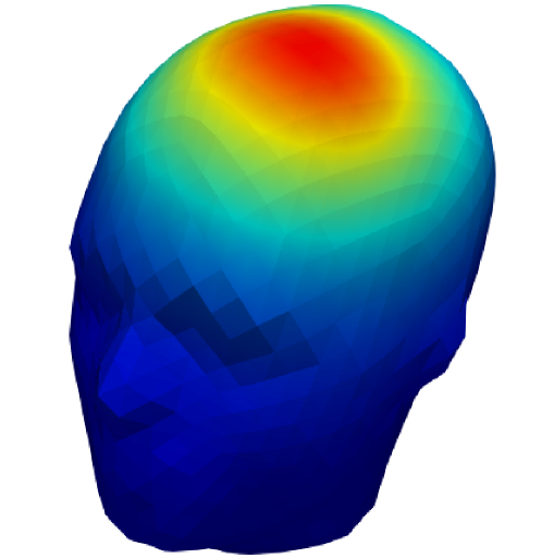
Figure 2: Scalp potential on an MRI-derived mesh

The proposed method is also applied on real data to demonstrate its versatility in modeling anisotropy. We used MRI datasets and template models from the libraries [13, 14] to obtain realistic surface and volume meshes. The wire mesh of white matter is obtained from streamline tractography [15] and clustering [16] of the diffusion MRI data. The tessellated geometry is illustrated in Figure 2 and 3.

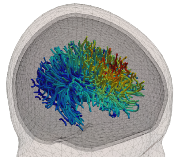
Figure 3: Fiber current on a tractography-generated mesh

The resulting solution along with a comparative DTI-based FEM model are computed and Figure 4 highlights the consistency between both methods as well as the impact of anisotropy modeling in the skull and in the white matter.

Figure 4: Electrode potential across different conductivity models

References

- [1] H. Hallez, B. Vanrumste, R. Grech, J. Muscat, W. De Clercq, A. Vergult, Y. D’Asseler, K. P. Camilleri, S. G. Fabri, S. Van Huffel et al., “Review on solving the forward problem in eeg source analysis,” Journal of neuroengineering and rehabilitation, vol. 4, no. 1, p. 46, 2007.
- [2] J. Kybic, M. Clerc, T. Abboud, O. Faugeras, R. Keriven, and T. Papadopoulo, “A common formalism for the integral formulations of the forward eeg problem,” IEEE transactions on medical imaging, vol. 24, no. 1, pp. 12–28, 2005.
- [3] J. Vorwerk, J.-H. Cho, S. Rampp, H. Hamer, T. R. Knösche, and C. H. Wolters, “A guideline for head volume conductor modeling in eeg and meg,” NeuroImage, vol. 100, pp. 590–607, 2014.
- [4] D. Le Bihan, “Looking into the functional architecture of the brain with diffusion mri,” Nature Reviews Neuroscience, vol. 4, no. 6, p. 469, 2003.
- [5] S. Shahid, P. Wen, and T. Ahfock, “Numerical investigation of white matter anisotropic conductivity in defining current distribution under tdcs,” Computer methods and programs in biomedicine, vol. 109, no. 1, pp. 48–64, 2013.
- [6] Y. Huang, A. A. Liu, B. Lafon, D. Friedman, M. Dayan, X. Wang, M. Bikson, W. K. Doyle, O. Devinsky, and L. C. Parra, “Measurements and models of electric fields in the in vivo human brain during transcranial electric stimulation,” Elife, vol. 6, p. e18834, 2017.
- [7] E. Olivi, T. Papadopoulo, and M. Clerc, “Handling white-matter anisotropy in bem for the eeg forward problem,” in Proceedings of the 8th IEEE International Symposium on Biomedical Imaging: From Nano to Macro, ISBI 2011., no. 799-802. IEEE, 2011, pp. 799–802.
- [8] A. Pillain, “Line, surface, and volume integral equations for the electromagnetic modelling of the electroencephalography forward problem,” Ph.D. dissertation, Ecole Nationale Supérieure des Télécommunications de Bretagne-ENSTB, 2016.
- [9] S. N. Makarov, A. Pascual-Leone, and A. Nummenmaa, “Modeling fiber-like conductivity structures via the boundary element method using thin-wire approximation. i construction of basis functions,” in 2016 38th Annual International Conference of the IEEE Engineering in Medicine and Biology Society (EMBC). IEEE, 2016, pp. 6473–6476.
- [10] L. Rahmouni, A. Pillain, A. Merlini, and F. P. Andriulli, “Integral equation modelling of brain fibers for handling white matter anisotropies in the eeg forward problem,” in 2017 International Conference on Electromagnetics in Advanced Applications (ICEAA). IEEE, 2017, pp. 1809–1812.
- [11] D. R. Wilton and N. J. Champagne, “Evaluation and integration of the thin wire kernel,” IEEE transactions on antennas and propagation, vol. 54, no. 4, pp. 1200–1206, 2006.
- [12] L. Rahmouni, R. Mitharwal, and F. P. Andriulli, “Two volume integral equations for the inhomogeneous and anisotropic forward problem in electroencephalography,” Journal of Computational Physics, vol. 348, pp. 732–743, 2017.
- [13] D. C. Van Essen, S. M. Smith, D. M. Barch, T. E. Behrens, E. Yacoub, K. Ugurbil, W.-M. H. Consortium et al., “The wu-minn human connectome project: an overview,” Neuroimage, vol. 80, pp. 62–79, 2013.
- [14] F. Tadel, S. Baillet, J. C. Mosher, D. Pantazis, and R. M. Leahy, “Brainstorm: a user-friendly application for meg/eeg analysis,” Computational intelligence and neuroscience, vol. 2011, p. 8, 2011.
- [15] J.-D. Tournier, F. Calamante, and A. Connelly, “Mrtrix: diffusion tractography in crossing fiber regions,” International Journal of Imaging Systems and Technology, vol. 22, no. 1, pp. 53–66, 2012.
- [16] E. Garyfallidis, M. Brett, M. M. Correia, G. B. Williams, and I. Nimmo-Smith, “Quickbundles, a method for tractography simplification,” Frontiers in neuroscience, vol. 6, p. 175, 2012.