Perturbation theory for operational quantum non-Markovianity

Abstract

The definition of memory in operational approaches to quantum non-Markovianity depends on the statistical properties of different sets of outcomes related to successive measurement processes performed over the system of interest. Using projectors techniques we develop a perturbation theory that enables to expressing both joint probabilities and outcome correlations in terms of the unperturbed system density matrix propagator. This object defines the open system dynamics in absence of measurement processes. Successive series terms, which are scaled by the system-environment interaction strength, consist in a convolution structure involving system propagators weighted by higher order bath correlations. The formalism is corroborated by studying different dynamics that admit an exact description. Using the perturbative approach, unusual memory effects induced by the interplay between the system-environment interaction and measurement processes are found in finite temperature reservoirs.

I Introduction

Most features characterizing an open quantum system dynamics can be recovered from a perturbative approach to the full system-environment dynamics. For example, the Born-Markov approximation (BMA) cohenbook ; breuerbook ; mandel is able to describe paradigmatic phenomena like decoherence and dissipation. Even more, quantum memory effects were originally related to departures from this “first-order” approximation vega ; wiseman . This association relies on the local-in-time property of the system evolution.

Over the past decade, the previous point of view was reviewed significantly. Instead of the BMA, the hallmark of quantum Markovianity becomes the theory of quantum dynamical semigroups alicki . In this alternative scenario BreuerReview ; plenioReview memory effects are determined from the system density matrix propagator, which in fact encode different departures that the system dynamics may develop with respect to a “Markovian” Lindblad dynamics BreuerFirst ; cirac ; rivas ; breuerDecayTLS ; fisher ; fidelity ; dario ; mutual ; geometrical ; DarioSabrina ; brasil ; sabrina ; canonicalCresser ; cresser ; paris ; Acin ; indu .

Alternative operational approaches ModiOperational  to quantum non-Markovianity have been introduced recently modi ; pollock ; pollockInfluence ; budiniCPF ; budiniChina ; budiniBrasil . Instead of focusing on mappings from density operators to density operators, the presence of memory is determined from the statistical properties of different outcomes obtained from successive measurement processes performed during the system evolution. Consistence with the classical definition of non-Markovianity is achieved. In fact, given a sequence of measurement outcomes, Markovianity can be checked through the corresponding conditional probabilities modi . In addition and in contrast to previous non-operational approaches, any possible dynamical departure from BMA renders the dynamic non-Markovian budiniCPF . Experimental setups for measuring memory in an operational way were implemented recently in Refs. budiniChina ; budiniBrasil .

The definition of quantum non-Markovianity from an operational perspective leads to an intrinsic dependence of memory effects on measurement processes, which leads to a richer structure when compared to the classical (incoherent) case pollock ; pollockInfluence ; budiniChina . On the other hand, in contrast to non-operational approaches where memory effects can be related to the system propagator, it is not known which physical object (or structure) may play the same role in these operational approaches budiniBrasil ; goan . In fact, the system dynamic between successive measurements, due to non-Markovian effects, cannot in general be described through a unique system propagator. This property has its physical origin in the modification or dependence of the bath state on system outcomes budiniCPF . The main goal of this paper is to provide a rigorous answer to this problem.

We characterize the structure that determines memory effects in operational approaches to quantum non-Markovianity. The study is valid for arbitrary system-environment interactions and relies on a perturbation theory formulated with projector operator techniques breuerbook ; projectors . The formalism is developed in the case where three system measurement processes are performed, being applied to both joint probabilities modi and a conditional past-future (CPF) correlation budiniCPF . In order to understand the intrinsic differences between operational and non-operational approaches, both kind of statistical objects are written as a function of the unperturbed system propagator, which defines the open system dynamics in absence of measurement processes. The projector approach naturally leads to an expansion series in the system-environment coupling strength. We found that successive order contributions consist in a convolution term involving two system propagators weighed by higher order bath correlations. This structure arises for both quantum and classical environmental fluctuations. These finding generalize the results found in budiniBrasil , which were derived for specific system-bath interaction Hamiltonians. The validity of the formalism is confirmed by studying different dynamics that admit an exact treatment such as dephasing and decay in a bosonic bath at zero temperature. As an application, we study memory effects in the thermalization of a two-level system, showing that unusual memory effects may be induced by raising the environment temperature. Generalization to arbitrary number of measurement processes follows straightforwardly from the present results.

The paper is outlined as follows. In Sec. II we review how memory effects can be determined from joint probabilities and the CPF correlation. In Sec. III we develop the perturbation theory for both classical and quantum environment fluctuations. In Sec. IV we apply the perturbation theory to dynamics that admit an exact treatment. In addition, we study memory effects induced by thermal reservoirs. In Sec. V we provide the Conclusions. Auxiliary calculation details are presented in the Appendix.

II Operational memory witnesses

Memory effects in open quantum systems can be determined by subjecting the system to successive measurement processes and checking if the corresponding probability structure satisfies the usual Markovian definition modi . It is simple to realize that a minimal number of three system observations is necessary to detect memory effects. Denoting with $x\rightarrow y\rightarrow z$ the successive measurement outcomes, their joint probability $P(z,y,x)$ can be written as

$$P(z,y,x)=P(z|y,x)P(y|x)P(x),$$ (1)

where in general, $P(b|a)$ denotes the conditional probability of $b$ given $a.$ Markovianity is defined by the equality $P(z,y,x)\overset{M}{=}P(z|y)P(y|x)P(x),$ that is, $P(z|y,x)\overset{M}{=}P(z|y).$ This property can easily be rewritten in terms of a conditional past-future independence, leading to the condition $P(z,x|y)\overset{M}{=}P(z|y)P(x|y).$ This last formulation can be checked with a CPF correlation budiniCPF ,

$$C_{pf}(t,\tau)|_{y}=\sum_{zx}[P(z,x|y)-P(z|y)P(x|y)]O_{z}O_{x}.$$ (2)

Thus, Markovianity implies $C_{pf}(t,\tau)|_{y}=0,$ while $C_{pf}(t,\tau)|_{y}\neq 0$ witnesses memory effects. In this equation, the sequence $\{x\}\rightarrow y\rightarrow\{z\}$ defines the outcomes at each stage, while $\{O_{z}\}$ and $\{O_{x}\}$ are the corresponding observables at the initial and final (past and future) observation times. The outcome $y$ gives the conditional character of the correlation. The parameters $t$ and $\tau$ denote the time intervals between the first and second, and between the second and third measurements, respectively.

Both operational memory witnesses [Eqs. (1) and (2)] can be mapped between them. Using that $P(z,x|y)=P(z,y,x)/P(y),$ $P(z|y)=P(z,y)/P(y)$ and $P(x|y)=P(y,x)/P(y),$ we get the equivalent expression

$$C_{pf}(t,\tau)|_{y}=\sum_{zx}\frac{O_{z}O_{x}}{P^{2}(y)}[P(z,y,x)P(y)-P(z,y)P(y,x)].$$ (3)

Here, all statistical objects can be written in terms of the joint probability $P(z,y,x).$ In fact, $P(z,y)=\sum_{x}P(z,y,x),$ $P(y,x)=\sum_{z}P(z,y,x)$ and $P(y)=\sum_{z,x}P(z,y,x).$

In a quantum regime, joint probabilities as well as the CPF correlation intrinsically depend on the chosen observables. Here they are defined through a set of measurement operators denoted as $\{\Omega_{x}\},$ $\{\Omega_{y}\},$ and $\{\Omega_{z}\},$ being normalized to the system identity matrix, $\sum_{z}\Omega_{z}^{\dagger}\Omega_{z}=\sum_{y}\Omega_{y}^{\dagger}\Omega_{y}=\sum_{x}\Omega_{x}^{\dagger}\Omega_{x}=\mathrm{I}.$ For simplicity, the intermediate measurement is assumed a projective one modi ; budiniCPF , that is, $\Omega_{y}^{\dagger}\Omega_{y}=\Omega_{y}.$

For the explicit calculation of $P(z,y,x)$ or $C_{pf}(t,\tau)|_{y}$ we must define the evolution of the system-environment arrange between measurements. Both (total) unitary dynamics and stochastic Liouville dynamics are considered.

II.1 Unitary system-environment dynamics

First, we assume that the system and the environment are described by a unitary evolution with Hamiltonian $H_{T}.$ The total density matrix $\rho_{t}^{se}$ evolves as

$$\frac{d}{dt}\rho_{t}^{se}=\mathcal{L}_{se}(t)[\rho_{t}^{se}],\ \ \ \ \ \ \ \mathcal{L}_{se}(t)[\bullet]=-i[H_{T}(t),\bullet].$$ (4)

As usual, the total Hamiltonian is written as $H_{T}(t)=H_{s}+H_{e}+H_{I}.$ Each contribution corresponds to the system, the environment, and their interaction Hamiltonian, respectively. The previous equation can be integrated as $\rho_{t}^{se}=\mathcal{E}_{t,0}[\rho_{0}^{se}],$ where the bipartite propagator is

$$\mathcal{E}_{t_{b},t_{a}}\equiv\left\lceil\exp\int_{t_{a}}^{t_{b}}dt^{\prime}\mathcal{L}_{se}(t^{\prime})\right\rceil.$$ (5)

Here $\left\lceil\cdots\right\rceil$ denotes a time ordering operation, which is necessary due to the dependence of $\mathcal{L}_{se}(t)$ on time. This case arises, for example, when working in an interaction representation or when the system is submitted to an external time dependent field.

The system density matrix follows from a partial trace over the environmental degrees of freedom, $\rho_{t}=\mathrm{Tr}_{e}(\rho_{t}^{se}).$ Thus,

$$\rho_{t}=\Lambda_{t,t_{0}}[\rho_{0}]\equiv\mathrm{Tr}_{e}(\mathcal{E}_{t,t_{0}}[\rho_{0}\otimes\sigma_{e}]),$$ (6)

where $\Lambda_{t,t_{0}}$ is the system density matrix propagator. For simplicity, we assume $t_{0}=0$ and separable initial conditions, $\rho_{0}^{se}=\rho_{0}\otimes\sigma_{e}.$

From standard quantum measurement theory, the expression for the 3-joint probability is suple

$$P(z,y,x)=\mathrm{Tr}_{se}(E_{z}\mathcal{E}_{t+\tau,t}[\rho_{y}\otimes\mathrm{Tr}_{s}(E_{y}\mathcal{E}_{t,0}[\tilde{\rho}_{x}\otimes\sigma_{e}])]),$$ (7)

where $\tilde{\rho}_{x}\equiv\Omega_{x}\rho_{0}\Omega_{x}^{\dagger}$ and $E_{i}\equiv\Omega_{i}^{{\dagger}}\Omega_{i}.$ Furthermore, $\rho_{y}=E_{y}$ is the (collapsed) system state after the second measurement. We notice that in Eq. (7) the evolution in the interval $(0,t)$ can be written in terms of the unperturbed system propagator $\Lambda_{t,0}$ defined in Eq. (6). Nevertheless, this object is insufficient to describe the dynamics in the interval $(t,t+\tau)$ because the initial bath state does not remain unchanged, $\sigma_{e}\rightarrow\mathrm{Tr}_{s}(E_{y}\mathcal{E}_{t,0}[\tilde{\rho}_{x}\otimes\sigma_{e}]).$ In fact, this feature is a witness of memory effects budiniCPF  whose description, for arbitrary system-environment interactions, is performed in the following section.

From Eq. (7), the CPF correlation [Eq. (3)] can be written as

$$C_{pf}(t,\tau)|_{y}=\frac{1}{P^{2}(y)}\sum_{zx}O_{z}O_{x}\mathrm{Tr}_{se}(E_{z}\mathcal{E}_{t+\tau,t}[\rho_{y}\otimes\mathrm{Tr}_{s}(E_{y}\mathcal{E}_{t,0}[\tilde{\rho}_{yx}\otimes\sigma_{e}])]),$$ (8)

where the auxiliary system matrix $\tilde{\rho}_{yx}$ is defined as $\tilde{\rho}_{yx}\equiv\tilde{\rho}_{x}\ P(y)-\tilde{\rho}\ P(y,x),$ being $\tilde{\rho}\equiv\sum_{x^{\prime}}\tilde{\rho}_{x^{\prime}}.$ Explicitly, it reads

$$\tilde{\rho}_{yx}=\tilde{\rho}_{x}\ \mathrm{Tr}_{s}(E_{y}\Lambda_{t,0}[\tilde{\rho}])-\tilde{\rho}\ \mathrm{Tr}_{s}(E_{y}\Lambda_{t,0}[\tilde{\rho}_{x}]),$$ (9)

Similarly, the probability $P(y)$ is given by

$$P(y)=\sum_{x^{\prime}}\mathrm{Tr}_{s}(E_{y}\Lambda_{t,0}[\tilde{\rho}_{x^{\prime}}]).$$ (10)

From the previous two expressions, we notice that both $\tilde{\rho}_{yx}$ and $P(y)$ can be written in terms of the unperturbed system propagator $\Lambda_{t,0}.$ On the other hand, it is simple to show that the matrix $\tilde{\rho}_{yx}$ never vanishes. In fact, after a simple algebra the condition $\tilde{\rho}_{yx}=0$ leads to the incongruence $\tilde{\rho}_{x}/P(x)=\tilde{\rho}.$

We notice that Eq. (8), disregarding the sum operation and under the replacement $\tilde{\rho}_{yx}\rightarrow\tilde{\rho}_{x},$ has the same structure as Eq. (7). This similitude allows us to formulate a perturbation theory that straightforwardly applies to both kinds of objects. The same relation is also valid for higher statistical objects (Sec. IV-C).

II.2 Stochastic Liouville dynamics

In addition, we deal with the case in which the open system evolution is defined by a stochastic Liouville dynamics,

$$\frac{d}{dt}\rho_{t}^{st}=\mathcal{L}_{st}(t)[\rho_{t}^{st}],\ \ \ \ \ \mathcal{L}_{st}(t)[\bullet]=-i[H_{st}(t),\bullet].$$ (11)

This equation can be integrated as $\rho_{t}^{st}=\mathcal{E}_{t,0}^{st}\rho_{0},$ where the stochastic propagator is

$$\mathcal{E}_{t_{b},t_{a}}^{st}\equiv\left\lceil\exp\int_{t_{a}}^{t_{b}}dt^{\prime}\mathcal{L}_{st}(t^{\prime})\right\rceil.$$ (12)

As before, $\left\lceil\cdots\right\rceil$ denotes a time ordering operation. The system density matrix $\rho_{t}=\overline{\rho_{t}^{st}}$ follows after averaging over realizations (over bar symbol) of the stochastic Liouville superoperator $\mathcal{L}_{st}(t).$ Thus,

$$\rho_{t}=\Lambda_{t,t_{0}}[\rho_{0}]\equiv\overline{\mathcal{E}_{t,t_{0}}^{st}}[\rho_{0}],$$ (13)

where for simplicity we assumed that the initial system state $\rho_{0}$ is uncorrelated from the noise fluctuations. As before, $\Lambda_{t,t_{0}}$ $(t_{0}=0)$ is the system density matrix propagator.

From quantum measurement theory, it is possible to obtain suple

$$P(z,y,x)=\overline{\mathrm{Tr}_{s}(E_{z}\mathcal{E}_{t+\tau,t}^{st}[\rho_{y}])\mathrm{Tr}_{s}(E_{y}\mathcal{E}_{t,0}^{st}[\tilde{\rho}_{x}])},$$ (14)

where, as before, $\tilde{\rho}_{x}=\Omega_{x}\rho_{0}\Omega_{x}^{\dagger}$ and $E_{i}=\Omega_{i}^{{\dagger}}\Omega_{i}.$ Similarly to the unitary case, here the (average) evolution in the interval $(0,t)$ can be written in terms of the unperturbed propagator (6), but it is unable to describe the dynamics in the interval $(t,t+\tau)$ because the system state at time $t$ is a random one, being correlated with the environmental fluctuations.

From Eq. (14) it is possible to write the CPF correlation [Eq. (3)] as

$$C_{pf}(t,\tau)|_{y}=\!\sum_{zx}\frac{O_{z}O_{x}}{P^{2}(y)}\overline{\mathrm{Tr}_{s}(E_{z}\mathcal{E}_{t+\tau,t}^{st}[\rho_{y}])\mathrm{Tr}_{s}(E_{y}\mathcal{E}_{t,0}^{st}[\tilde{\rho}_{yx}])},$$ (15)

where $\tilde{\rho}_{yx}$ and $P(y)$ can be read from Eqs. (9) and (10), respectively, with the propagator $\Lambda_{t,0}$ defined by Eq. (13).

Here, we can see that Eqs. (14) and (15) present a similar structure, and both expressions can be related under the same mapping that connects Eqs. (7) and (8).

III Perturbation theory

In non-operational memory approaches, memory effects are mainly determined from the unperturbed system density propagator. Thus, we develop a perturbation theory where this object remains as an input of the formalism. For both unitary system-environment interactions as well as stochastic Liouville dynamics the formalism is developed using projector techniques, which allow us to find exact series expansions of both the joint probability $P(z,y,x)$ and the CPF correlation $C_{pf}(t,\tau)|_{y}.$

III.1 Unitary system-environment dynamics

We introduce standard projectors projectors

$$\mathcal{P}[\rho_{se}]=\mathrm{Tr}_{e}(\rho_{se})\otimes\sigma_{e},\ \ \ \ \ \mathcal{Q}[\rho_{se}]=\rho_{se}-\mathrm{Tr}_{e}(\rho_{se})\otimes\sigma_{e},$$ (16)

where $\sigma_{e}$ is a reference state of the bath. They satisfy $\mathcal{P}+\mathcal{Q}=\mathrm{I}_{se},$ where $\mathrm{I}_{se}$ is the bipartite identity matrix. Introducing the operator $\mathrm{I}_{se}$ in front of each propagator $\mathcal{E}$ in Eq. (7), it follows

$$\begin{array}[b]{r}P(z,y,x)\!=\!\mathrm{Tr}_{se}(E_{z}\mathcal{PE}_{t+\tau,t}[\rho_{y}\!\otimes\!\mathrm{Tr}_{s}(E_{y}\mathcal{PE}_{t,0}[\tilde{\rho}_{x}\otimes\sigma_{e}])])\\ \\ \!+\mathrm{Tr}_{se}(E_{z}\mathcal{PE}_{t+\tau,t}[\rho_{y}\!\otimes\!\mathrm{Tr}_{s}(E_{y}\mathcal{QE}_{t,0}[\tilde{\rho}_{x}\otimes\sigma_{e}])]).\end{array}$$ (17)

In deriving this expression we used that $\mathrm{Tr}_{e}(\mathcal{Q}[\rho_{se}])=0,$ equality valid for arbitrary system-environment state $\rho_{se}.$ We notice that the first line in the previous equation can be written in terms of two system propagators [Eq. (6)] between two arbitrary times, $\Lambda_{t,t^{\prime}}[\rho]=\mathrm{Tr}_{e}(\mathcal{E}_{t,t^{\prime}}[\rho\otimes\sigma_{e}]).$ In the second line, as usual, we note that for separable initial conditions the irrelevant part in the projector technique can be integrated as (see Appendix)

$$\mathcal{QE}_{t_{b},t_{a}}=\int_{t_{a}}^{t_{b}}dt^{\prime}\mathcal{G}_{t,t^{\prime}}\mathcal{QL}_{se}(t^{\prime})\mathcal{PE}_{t^{\prime},t_{a}},$$ (18)

where

$$\mathcal{G}_{t,t^{\prime}}\equiv\left\lceil\exp\int_{t^{\prime}}^{t}d\tau^{\prime}\mathcal{QL}_{se}(\tau^{\prime})\right\rceil.$$ (19)

Therefore, the contribution proportional to $\mathcal{QE}_{t_{b},t_{a}}^{st}$ in Eq. (17) can also be written in terms of the unperturbed propagator $\mathcal{PE}_{t^{\prime},t_{a}}[\rho\otimes\sigma_{e}]$ [Eq. (6)]. On the other hand, the relevant part (in the second line) can also be integrated as (see Appendix)

$$\mathcal{PE}_{t_{b},t_{a}}=\mathcal{PE}_{t_{b},t_{a}}\mathcal{P}\!+\!\int_{t_{a}}^{t_{b}}dt^{\prime}\mathcal{PE}_{t_{b},t^{\prime}}\mathcal{P\mathcal{L}}_{se}(t^{\prime})\mathcal{G}_{t^{\prime},t_{a}}\mathcal{Q}.$$ (20)

This expression is of central importance for the developing of the formalism because it enables to characterize the projected system dynamics in terms of the unperturbed propagator even when considering arbitrary initial environment states.

Introducing explicitly Eqs. (18) and (20) in $P(z,y,x),$ using that $\mathcal{PQ}=0$ and after some algebra, from Eq. (17) we get

$$P(z,y,x)\!=\!\mathrm{Tr}_{s}(E_{z}\Lambda_{t+\tau,t}[\rho_{y}])\mathrm{Tr}_{s}(E_{y}\Lambda_{t,0}[\tilde{\rho}_{x}])+\int_{0}^{\tau}\!\!\!d\tau^{\prime}\int_{0}^{t}\!\!\!dt^{\prime}\mathrm{Tr}_{s}(E_{z}\Lambda_{t+\tau,t+\tau^{\prime}}\mathrm{Tr}_{e}(\tilde{\Phi}_{t+\tau^{\prime},t}^{se}[\rho_{y}\otimes\mathrm{Tr}_{s}(E_{y}\Phi_{t,t^{\prime}}^{se}\Lambda_{t^{\prime},0}[\tilde{\rho}_{x}]\otimes\sigma_{e})])),$$ (21)

where for shortening the expression we introduced the system-environment superoperators

$$\tilde{\Phi}_{t_{b},t_{a}}^{se}=\mathcal{\mathcal{L}}_{se}(t_{b})\mathcal{G}_{t_{b},t_{a}},\ \ \ \ \ \ \ \ \Phi_{t_{b},t_{a}}^{se}\equiv\mathcal{G}_{t_{b},t_{a}}\mathcal{QL}_{se}(t_{a}).$$ (22)

The system propagator $\Lambda_{t,t^{\prime}}$ is defined by Eq. (6).

Eq. (21) is the main result of this section. It expresses $P(z,y,x)$ as a function of the unperturbed system propagator. We notice that the first contribution corresponds to a Markovian limit, where $P(z,y,x)\overset{M}{=}P(z|y)P(y|x)P(x)$ with $P(z|y)\overset{M}{=}\mathrm{Tr}_{s}(E_{z}\Lambda_{t+\tau,t}[\rho_{y}])$ and $P(y|x)P(x)\overset{M}{=}\mathrm{Tr}_{s}(E_{y}\Lambda_{t,0}[\tilde{\rho}_{x}])$ with $P(x)=\mathrm{Tr}_{s}(\tilde{\rho}_{x})=\mathrm{Tr}_{s}(E_{x}\rho_{0}).$ Consistently, the second (integral) contribution takes into account memory effects, which in turn answers our main motivation. It consists in a convolution structure involving two unperturbed system propagators weighted by the “correlation” between the bipartite operators $\tilde{\Phi}_{t_{b},t_{a}}^{se}$ and $\Phi_{t_{b},t_{a}}^{se}$ [Eq. (22)]. These objects can be written as a series in the interaction strength [proportional to $\mathcal{\mathcal{L}}_{se}(t)],$ which follows from the expansion $\mathcal{G}_{t,t^{\prime}}=\mathrm{I}_{se}+\int_{t^{\prime}}^{t}d\tau_{1}\mathcal{QL}_{se}(\tau_{1})+\int_{t^{\prime}}^{t}d\tau_{2}\int_{t^{\prime}}^{\tau_{2}}d\tau_{1}\mathcal{QL}_{se}(\tau_{2})\mathcal{QL}_{se}(\tau_{1})+\cdots.$ Thus, the non-Markovian contribution in Eq. (21) can be written as a series in the interaction strength, each term involving two system propagators and high order bath correlations.

In order to lighten the structure of the perturbation series, we write it for the CPF correlation. Using the similarity between Eqs. (7) and (8), it follows that the first (Markovian) term in Eq. (21) does not contribute to $C_{pf}(t,\tau)|_{y}.$ In fact $\sum_{x}O_{x}\mathrm{Tr}_{s}(E_{y}\Lambda_{t,0}[\tilde{\rho}_{yx}])=0.$ Thus, consistently the CPF correlation only depends on the second integral contribution, which in fact measures the memory effects. We get

$$C_{pf}(t,\tau)|_{y}=\sum_{z,x}\frac{O_{z}O_{x}}{P^{2}(y)}\int_{0}^{t}dt^{\prime}\int_{0}^{\tau}d\tau^{\prime}\Xi(z,x|y)[\tilde{\rho}_{yx}],$$ (23)

where

$$\Xi(z,x|y)[\bullet]\equiv\mathrm{Tr}_{se}(E_{z}\tilde{\Upsilon}_{t+\tau^{\prime},t}^{se}[\ \rho_{y}\otimes\mathrm{Tr}_{s}(E_{y}\Upsilon_{t,t^{\prime}}^{se}[\bullet])\ ]).$$ (24)

This term defines the integrand in Eq. (21). For notational convenience here we introduced the superoperator

$$\tilde{\Upsilon}_{t+\tau^{\prime},t}^{se}[\bullet]\equiv\Lambda_{t+\tau,t+\tau^{\prime}}\tilde{\Phi}_{t+\tau^{\prime},t}^{se}[\bullet],$$ (25)

and similarly

$$\Upsilon_{t,t^{\prime}}^{se}[\bullet]\equiv\Phi_{t,t^{\prime}}^{se}[\Lambda_{t^{\prime},0}[\bullet]\otimes\sigma_{e}].$$ (26)

The final expression (23) enables to perform a perturbative theory for the CPF correlation developed as a series in terms of the system-environment interaction strength. In fact, expansion of the superoperators $\tilde{\Phi}_{t_{b},t_{a}}^{se}$ and $\Phi_{t_{b},t_{a}}^{se}$ [Eq. (22)] in powers of $\mathcal{\mathcal{L}}_{se}(t)$ leads to

$$\Xi(z,x|y)[\bullet]=\sum_{n=1}^{\infty}\Xi^{(n)}(z,x|y)[\bullet],$$ (27)

where the index $n$ labels the bath correlation order that appears in each term. For example, to first order $\tilde{\Phi}_{t_{b},t_{a}}^{se}=\mathcal{\mathcal{L}}_{se}(t_{b})\mathcal{G}_{t_{b},t_{a}}\simeq\mathcal{\mathcal{L}}_{se}(t_{b}),$ and $\Phi_{t_{b},t_{a}}^{st}=\mathcal{G}_{t_{a},t_{b}}^{st}\mathcal{QL}_{se}(t_{a})\simeq\mathcal{QL}_{se}(t_{a})=\mathcal{L}_{se}(t_{a}),$ where the last equality relies on the usual assumption $\mathcal{PL}_{se}(t_{a})\mathcal{P}=0.$ The first not null order is weighted by the bath correlations $\mathrm{Tr}_{e}(\mathcal{L}_{se}(t)\mathcal{L}_{se}(t^{\prime})\sigma_{e}),$ which in turn weights the integral between both system propagators $\Lambda_{t+\tau,t+\tau^{\prime}}$ and $\Lambda_{t^{\prime},0}.$ This structure is similar to that found in Ref. budiniBrasil for models that admit an exact analytic calculation.

In order to explicitly visualize the previous structure, we consider the bipartite Hamiltonian

$$H_{T}(t)=\sum_{\mu}S_{t}^{\mu}\otimes B_{t}^{\mu}.$$ (28)

Assuming, as usual, that expectation values of the bath operators are null, $\mathrm{Tr}_{e}(B_{t}^{\mu}\sigma_{e})=0,$ and considering Hermitian operators, from Eq. (24) we get

$$\begin{array}[]{r}\Xi^{(1)}(z,x|y)[\bullet]=\sum\limits_{\mu,\nu}\Big{\{}\mathrm{Tr}_{s}\Big{(}E_{z}\Lambda_{t+\tau,t+\tau^{\prime}}[\rho_{y}S_{t+\tau^{\prime}}^{\mu}]\Big{)}-c.c.\Big{\}}\\ \\ \!\!\!\!\!\!\!\!\times\Big{\{}\chi_{\mu\nu}(\tau^{\prime}+t^{\prime})\ \mathrm{Tr}_{s}\Big{(}E_{y}S_{t-t^{\prime}}^{\nu}\Lambda_{t^{\prime},0}[\bullet]\Big{)}-c.c.\Big{\}},\end{array}$$ (29)

where the bath correlations are defined as $\chi_{\mu\nu}(t,t^{\prime})\equiv\mathrm{Tr}_{e}(B_{t}^{\mu}B_{t^{\prime}}^{\nu}\sigma_{e}).$ For simplicity they are assumed stationary, $\chi_{\mu\nu}(t+\tau^{\prime},t-t^{\prime})=\chi_{\mu\nu}(\tau^{\prime}+t^{\prime}).$ Higher order terms include higher bath correlations that involve a higher number of bath operators. For bosonic environments, $\Xi^{(n)}(z,x|y)[\bullet]$ involves a product of $n$ correlations $\chi_{\mu\nu}(t,t^{\prime}).$ When $\chi_{\mu\nu}(\tau^{\prime}+t^{\prime})\approx\delta(\tau^{\prime}+t^{\prime}),$ the double time integral $\int_{0}^{t}dt^{\prime}\int_{0}^{\tau}d\tau^{\prime}$ of the successive series terms vanishes, recovering consistently a Markovian limit.

We remark that the exact expressions (21) and (23) explicitly depend on the unperturbed propagator $\Lambda_{t_{b},t_{a}}.$ This object, when is not available in an exact analytical way, using standard tools breuerbook ; projectors , can be approximated to the same order as the joint probability or CPF correlation.

III.2 Stochastic Liouville dynamics

The previous perturbation theory can also be developed for the case of stochastic Liouville dynamics, Eqs. (14) and (15). Instead of the projectors (16), here they are defined as

$$\mathcal{P}[f_{st}]=\overline{f_{st}},\ \ \ \ \ \ \ \ \ \mathcal{Q}[f_{st}]=f_{st}-\overline{f_{st}},$$ (30)

where $f_{st}$ is an arbitrary functional of the noise fluctuations. After introducing the identity $\mathcal{P}+\mathcal{Q}=1$ in Eq. (14), we get

$$\begin{array}[]{r}P(z,y,x)=\overline{\mathrm{Tr}_{s}(E_{z}\mathcal{PE}_{t+\tau,t}^{st}[\rho_{y}])\mathrm{Tr}_{s}(E_{y}\mathcal{PE}_{t,0}^{st}[\tilde{\rho}_{x}])}\\ \\ +\overline{\mathrm{Tr}_{s}(E_{z}\mathcal{PE}_{t+\tau,t}^{st}[\rho_{y}])\mathrm{Tr}_{s}(E_{y}\mathcal{QE}_{t,0}^{st}[\tilde{\rho}_{x}])}.\end{array}$$ (31)

Using similar transformations and solutions as in the previous section, for the joint probability we obtain

$$P(z,y,x)\!=\!\mathrm{Tr}_{s}(E_{z}\Lambda_{t+\tau,t}[\rho_{y}])\mathrm{Tr}_{s}(E_{y}\Lambda_{t,0}[\tilde{\rho}_{x}])+\int_{0}^{\tau}d\tau^{\prime}\int_{0}^{t}dt^{\prime}\overline{\mathrm{Tr}_{s}(E_{z}\Lambda_{t+\tau,t+\tau^{\prime}}\tilde{\Phi}_{t+\tau^{\prime},t}^{st}[\rho_{y}])\mathrm{Tr}_{s}(E_{y}\Phi_{t,t^{\prime}}^{st}\Lambda_{t^{\prime},0}[\tilde{\rho}_{x}])]},$$ (32)

where here

$$\tilde{\Phi}_{t_{b},t_{a}}^{st}=\mathcal{\mathcal{L}}_{st}(t_{b})\mathcal{G}_{t_{b},t_{a}}^{st},\ \ \ \ \ \ \ \ \Phi_{t_{b},t_{a}}^{st}\equiv\mathcal{G}_{t_{b},t_{a}}^{st}\mathcal{QL}_{st}(t_{a}),$$ (33)

and correspondingly

$$\mathcal{G}_{t,t^{\prime}}^{st}=\left\lceil\exp\int_{t^{\prime}}^{t}dt^{\prime}\mathcal{QL}_{st}(t^{\prime})\right\rceil.$$ (34)

The propagator $\Lambda_{t_{b},t_{a}}$ is defined by Eq. (13). The CPF correlation, using the similitude of Eqs. (14) and (15), can be written from Eq. (32) as

$$C_{pf}(t,\tau)|_{y}=\sum_{z,x}\frac{O_{z}O_{x}}{P^{2}(y)}\int_{0}^{t}dt^{\prime}\int_{0}^{\tau}d\tau^{\prime}\overline{\Xi(z,x|y)}[\tilde{\rho}_{yx}],$$ (35)

where

$$\overline{\Xi(z,x|y)}[\bullet]\equiv\overline{\mathrm{Tr}_{s}(E_{z}\tilde{\Upsilon}_{t+\tau^{\prime},t}^{st}[\rho_{y}])\mathrm{Tr}_{s}(E_{y}\Upsilon_{t,t^{\prime}}^{st}[\bullet])}.$$ (36)

Similarly, we defined

$$\tilde{\Upsilon}_{t+\tau^{\prime},t}^{st}[\bullet]\equiv\Lambda_{t+\tau,t+\tau^{\prime}}\tilde{\Phi}_{t+\tau^{\prime},t}^{st}[\bullet],$$ (37)

and the stochastic superoperator

$$\Upsilon_{t,t^{\prime}}^{st}[\bullet]\equiv\Phi_{t,t^{\prime}}^{st}[\Lambda_{t^{\prime},0}[\bullet]].$$ (38)

Furthermore, $\rho_{yx}$ is the matrix defined by Eq. (9). From Eq. (36) the perturbation theory follows straightforwardly.

IV Examples and applications

In this section we apply the perturbation theory for different dynamics of interest such as dephasing induced by a Gaussian non-white noise and dissipation induced by a non-Markovian bosonic thermal bath.

IV.1 Non-Markovian dephasing

We consider a two-level system driven by a dephasing stochastic Hamiltonian. The stochastic system state $\rho_{t}^{st}$ evolves as

$$\frac{d}{dt}\rho_{t}^{st}=-i\xi(t)[\sigma_{\hat{z}},\rho_{t}^{st}],$$ (39)

where $\sigma_{\hat{z}}$ is the $\hat{z}$-Pauli matrix (eigenvalues $|\pm\rangle$) and $\xi(t)$ is a (real) stationary color Gaussian noise with vanishing average $\overline{\xi(t)}=0$ and stationary correlation $\chi(t-t^{\prime})=\overline{\xi(t)\xi(t^{\prime})}=(\gamma/2\tau_{c})\exp[-|t-t^{\prime}|/\tau_{c}].$ We consider that the system begins in its upper state, $\rho_{0}=|+\rangle\langle+|.$ Furthermore, the three measurements are performed in the $\hat{x}$-direction in the Bloch sphere, $\{\Omega_{x}\}=\{\Omega_{y}\}=\{\Omega_{z}\}=|\hat{x}_{\pm}\rangle\langle\hat{x}_{\pm}|,$ where $|\hat{x}_{\pm}\rangle=(|+\rangle\pm|-\rangle)/\sqrt{2}$ are the eigenvalues of $\sigma_{\hat{x}},$ the $\hat{x}$-Pauli matrix. Thus, $x=\pm 1,$ $y=\pm 1,$ and $z=\pm 1.$ Under the previous conditions, both the joint probabilities and CPF correlation can be obtained in an exact analytical way. Explicit expressions can be found in Ref. budiniCPF $[(\gamma/2\tau_{c})\leftrightarrow g^{2}].$ Similarly, for this model it is possible to obtain explicit recursive relations and expressions for the successive series terms [Eq. (27)], which are of order $(\gamma\tau_{c})^{n}.$ Due to the symmetry of the problem, the first order contribution vanishes.

In Fig. 1 we plot the CPF correlation $C_{pf}(t,\tau)|_{y}$ at equal measurement time intervals $t=\tau$, for different noise correlation times. Both the exact expression and the perturbation theory estimation are shown. The unperturbed system propagator $\Lambda_{t,t^{\prime}}$ [Eq. (13)] was taken as the exact one. Similarly to the exact expression, the CPF correlation obtained by adding successive series terms is independent of the conditional $y=\pm 1.$ We found that for smaller noise correlation times the convergence to the exact expression is increased, which shows the consistence of the perturbation theory. Furthermore, we checked that, to the same order, all joint probabilities $P(z,y,x)$ [Eq. (32)] are definite positive. This feature also supports the developed formalism.

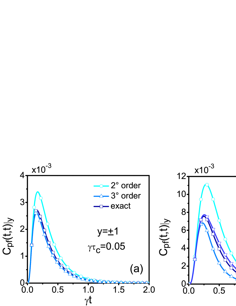
Figure 1: CPF correlation $C_{pf}(t,t)|_{y}$ $(y=\pm 1)$ obtained by adding successive contributions in the perturbation theory for the dephasing dynamics (39). The noise correlation is $\chi(t)=(\gamma/2\tau_{c})\exp[-|t|/\tau_{c}].$ The three measurements are performed in the $\hat{x}$-Bloch direction, while the system begins in its upper state. The parameters in (a) and (b) respectively are $\gamma\tau_{c}=0.05\$and $0.1.$

IV.2 Non-Markovian bosonic bath

The decay of a two-level system in a bosonic environment is described by the total Hamiltonian breuerbook

$$H_{\mathrm{tot}}=\frac{\omega_{0}}{2}\sigma_{z}+\sum_{k}\omega_{k}b_{k}^{{\dagger}}b_{k}+\sum_{k}(g_{k}\sigma_{+}b_{k}+g_{k}^{\ast}\sigma_{-}b_{k}^{{\dagger}}),$$ (40)

where $[b_{k},b_{k}^{{\dagger}}]=1$ are the creation-annihilation bosonic operators and $\sigma_{+}=|+\rangle\langle-|,$ $\sigma_{-}=|-\rangle\langle+|$ are the raising and lowering operators of the system. Memory effects in this dynamics can also be analyzed in an operational approach to quantum non-Markovianity.

We consider two different measurement schemes. In the first one, the three measurements are performed in $\hat{z}-$Bloch direction ($\hat{z}$-$\hat{z}$-$\hat{z}$ scheme) while in the second one, the first and last measurements are performed in the $\hat{x}-$Bloch direction, while the intermediate one in the $\hat{z}$-direction ($\hat{x}$-$\hat{z}$-$\hat{x}$ scheme). These observables are defined in the representation interaction with respect to the system and bath free evolutions. In this frame, the total Hamiltonian reads

$$H_{\mathrm{tot}}=\sigma_{+}B(t)+\sigma_{-}B^{\dagger}(t),$$ (41)

where $B(t)=\sum_{k}g_{k}b_{k}\exp[+i(\omega_{0}-\omega_{k})t].$ Furthermore, the initial bipartite state is taken as

$$\rho_{0}^{se}=|\psi_{0}\rangle\langle\psi_{0}|\otimes\sigma_{e},\ \ \ \ \ \ \ |\psi_{0}\rangle=(a|+\rangle+b|-\rangle),$$ (42)

with normalized coefficients $a$ and $b.$ The initial bath state $\sigma_{e}$ is taken as a thermal one. For both measurement schemes, the perturbation theory enables us to study the dependence of memory effects with temperature. Given the bosonic property of the bath, its complete set of (operator) correlations can be written in terms of only two ones,

$$\chi_{\downarrow}(t)\equiv\mathrm{Tr}_{e}[B(t)B^{\dagger}\sigma_{e}],\ \ \ \ \ \ \chi_{\uparrow}(t)\equiv\mathrm{Tr}_{e}[B^{\dagger}(t)B\sigma_{e}].$$ (43)

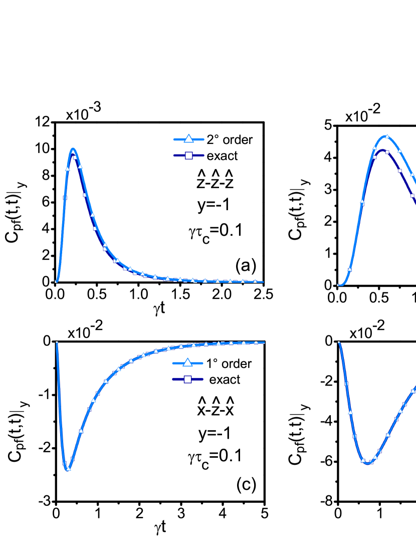
Figure 2: CPF correlation $C_{pf}(t,t)|_{y}$ $(y=-1)$ obtained in a perturbative way for the dissipative dynamics (41) with environment at zero temperature. Its correlations are $\chi_{\downarrow}(t)=(\gamma/2\tau_{c})\exp[-|t|/\tau_{c}]$ and $\chi_{\uparrow}(t)=0.$ (a) and (b) correspond to the $\hat{z}$-$\hat{z}$-$\hat{z}$ measurement scheme while (c) and (d) to the $\hat{x}$-$\hat{z}$-$\hat{x}$ scheme. The bath correlation time $\tau_{c}$ is indicated in each plot. In all cases, the initial system state is $|\psi_{0}\rangle=(\sqrt{p}|+\rangle+\sqrt{1-p}|-\rangle)$ with $p=0.8.$

Zero temperature: For different physical arrangements, the environment temperature can be (effectively) taken as null. Thus, $\sigma_{e}=|0\rangle\langle 0|,$ where $|0\rangle\equiv\prod_{k}|0\rangle_{k}.$ Each state $|0\rangle_{k}$ corresponds to the vacuum state of each bosonic mode. As is well known breuerbook , in this case the full system-environment dynamic admits a simple analytical solution, given also an exact expression for the unperturbed system propagator $\Lambda_{t,t^{\prime}}$ [Eq. (6)]. Furthermore, the CPF correlation and joint probabilities can also be calculated in an exact way. In fact, the open system dynamics and the CPF correlation have been implemented and measured in a photonic setup budiniBrasil .

We consider a Lorentzian spectral bath density. Thus, the environment correlations read $\chi_{\downarrow}(t)=(\gamma/2\tau_{c})\exp[-|t|/\tau_{c}],$ while the zero temperature condition leads to $\chi_{\uparrow}(t)=0.$ In Fig. 2 we plot the CPF correlation $C_{pf}(t,t)|_{y}$ at equal time intervals for both measurement schemes and the conditional $y=-1.$ In the $\hat{z}$-$\hat{z}$-$\hat{z}$ scheme [(a) and (b)], the first order contribution vanishes. Similarly to the previous case, (at second order) a decrease in the bath correlation time leads to a higher convergence with the exact analytical result budiniBrasil . On the other hand, in the $\hat{x}$-$\hat{z}$-$\hat{x}$ scheme, the first order contribution coincides with the exact solution. Thus, while higher order contributions do not vanish, their addition cancel out. These results also support the consistence of the perturbation theory. In addition, we found that to the same order, all joint probabilities $P(z,y,x)$ [Eq. (21)] are definite positive.

For the conditional $y=+1,$ the exact calculation of the CPF correlation leads to budiniBrasil

$$C_{pf}(t,\tau)|_{y=+1}\underset{\hat{z}\hat{z}\hat{z}}{=}0,\ \ \ \ \ \ \ \ C_{pf}(t,\tau)|_{y=+1}\underset{\hat{x}\hat{z}\hat{x}}{=}0.$$ (44)

In this case, the joint probabilities $P(z,y,x)$ can be written as $P(z,1,x)\underset{\hat{z}\hat{z}\hat{z}}{=}P(z|1)P(1|x)P(x)$and $P(z,1,x)\underset{\hat{x}\hat{z}\hat{x}}{=}P(z)P(1)P(x)$ probability . In fact, these expressions correspond to the first contribution in Eq. (21), while the integral contribution vanishes. Thus, in this restricted case $(y=+1),$ the Markov property is fulfilled leading to a vanishing CPF correlation and, consequently, the perturbation theory loses its meaning.

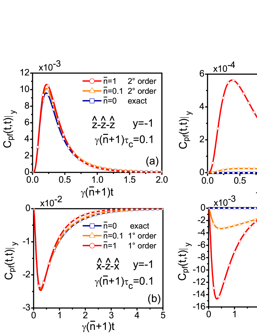
Figure 3: CPF correlation $C_{pf}(t,t)|_{y}$ obtained in a perturbative way for the dissipative dynamics (41) with an environment at finite temperature. Its correlations are $\chi_{\downarrow}(t)=(\bar{n}+1)(\gamma/2\tau_{c})\exp[-|t|/\tau_{c}]$ and $\chi_{\uparrow}(t)=\bar{n}(\gamma/2\tau_{c})\exp[-|t|/\tau_{c}].$ (a) and (b) correspond to $y=-1$ for the $\hat{z}$-$\hat{z}$-$\hat{z}$ and $\hat{x}$-$\hat{z}$-$\hat{x}$ measurement schemes, respectively. In (c) and (d) $y=+1.$ The bath correlation parameters are indicated in each plot. In all cases, the initial system state $|\psi_{0}\rangle$ is the same as in Fig. 2.

Finite temperature: For finite temperature, a simple expression for the unperturbed system propagator is not available. In addition, neither the CPF correlation nor the joint probabilities can be obtained in an exact analytical way. Nevertheless, this case can be dealt with the developed perturbation theory.

At finite temperature, both bath correlations [Eq. (43)] must be considered. As a model, we take $\chi_{\downarrow}(t)=(\bar{n}+1)(\gamma/2\tau_{c})\exp[-|t|/\tau_{c}],$ and $\chi_{\uparrow}(t)=\bar{n}(\gamma/2\tau_{c})\exp[-|t|/\tau_{c}],$ where $\bar{n}$ is the average number of bosonic bath excitations at the natural frequency of the system. When $\bar{n}=0$ the previous Lorentzian case at null temperature is recovered. This correlation model arises when the dependence on frequency of the number of thermal bath excitations is almost a flat function around the natural system frequency mandel . In this approximation, temperature increases the “intensity” of the environment fluctuations, while their correlation time is independent of it. Consistently, the unperturbed density matrix propagator is taken as the (exact) zero temperature propagator breuerbook , with an extra similar contribution that takes into account (thermally induced) transitions from the lower to the upper system state.

By using the previous assumptions, in Fig. 3 we plot the CPF correlation obtained from the perturbation theory [Eqs. (23) and (27)]. For both measurement schemes ($\hat{z}$-$\hat{z}$-$\hat{z}$ and $\hat{x}$-$\hat{z}$-$\hat{x}$), and for the conditional $y=-1$ [Figs. 3(a) and (b)], the memory effects (amplitude of the CPF correlation) weakly depends on temperature. Small departures with respect to the vanishing temperature case [Fig. 2] are observed. Due to the normalization of the time axis $[\gamma(\bar{n}+1)t],$ a natural change of time scale (shrinking due to the increasing of the effective system decay rates) is not observed.

On the other hand, for the conditional $y=+1$ [Figs. 3(c) and (d)] a strong dependence on temperature is observed in both measurement schemes. In fact, in this situation, in the limit $\bar{n}\rightarrow 0,$ the CPF correlation vanishes, Eq. (44). By increasing temperature the maximal amplitude of the CPF correlation also increases.

The previous unusual effect, that is, an increasing of the memory effects with temperature, does not rely on the specific environmental properties such as the proposed correlation model. It relies on the symmetries of the problem, which are defined by the system-environment interaction and the quantum measurement processes. For the conditional $y=+1,$ an increasing of the bath temperature leads to an extra dissipation channel that breaks the conditional statistical independence of the first and last (past and future) measurement outcomes. From the point of view of joint probabilities, temperature leads to extra contributions that break the Markovian property. In fact, for $y=+1$ we found that the first integral series contributions in Eq. (21) are proportional to $\bar{n},$ while in the previous case $(y=-1)$ are proportional to $(\bar{n}+1).$ We checked that by increasing temperature, the memory effects saturates. In addition, a vanishing of memory effects with temperature can be introduced through a temperature dependent bath correlation time.

IV.3 Generalizations

The present approach is generalizable to different cases of interest. First, the formalism can be extended by considering arbitrary initial conditions, $\rho_{0}^{se}\neq\rho_{0}\otimes\sigma_{e}.$ For example the bath state can be an arbitrary one, different from the reference state in the projectors definition [Eq. (16)]. In addition system and environment may be correlated at the initial time. These situations lead to an extra term in the perturbation theory [see Eq. (46) in the Appendix]. On the other hand, higher statistical objects can also be worked out with similar techniques. In fact, one may consider higher joint probabilities $P(x_{m},\cdots x_{1})$ involving $m$-measurement processes modi . In this case, $(m-1)$ system propagators are involved in the convolution term, while the structure of series terms assumes a similar form. The same result applies to higher CPF correlations budiniCPF .

V Summary and Conclusions

Using projector techniques, we have developed a perturbation theory for describing memory effects in operational approaches to quantum non-Markovianity, where the system dynamics is explicitly observed at different times. The formalism leads to exact expressions of both joint probabilities and correlations, which are written in terms of the unperturbed system density matrix propagator. We worked out the minimal case of three measurement processes. Memory contributions are defined by a convolution integral involving two system propagators, where the successive series terms are weighted by higher order bath correlations. In a bosonic or Gaussian case they can be reduced to two-point correlations. This result clarifies which structure determines memory effects in operational approaches to quantum non-Markovianity.

As examples, we applied the theory to different open system dynamics that admit an exact treatment, such as dephasing induced by stochastic Hamiltonians and decay of a two-level system in a bosonic reservoir at zero temperature. The consistence between the perturbation theory and exact solutions shows and guarantees the validity of the proposed approach. We also studied non-Markovian effects that emerge when considering thermal baths. Unusual memory effects arise due to the interplay between the measurement process, the bipartite dynamics, and the environment temperature. We found that, depending on the chosen measurement processes and conditionals, memory effects may grow with the environment temperature. This feature can be understood from a special interplay between the previous ingredients, where an extra dissipative channel induced by the environment temperature facilitates the developing of memory effects.

To conclude, our theory provides a solid basis for analyzing memory effects in operational approaches to quantum non-Markovianity. Application to others physical arrangements and statistical objects can be tackled by using the developed formalism.

Appendix A Formal solutions from projector techniques

As usual projectors , a bipartite system-environment evolution, $(d/dt)\rho_{t}^{se}=\mathcal{L}_{se}(t)\rho_{t}^{se},$ can be split as

$$\frac{d}{dt}\mathcal{P}\rho_{t}^{se} = \mathcal{PL}_{se}(t)\mathcal{P}\rho_{t}^{se}+\mathcal{PL}_{se}(t)\mathcal{Q}\rho_{t}^{se},$$ (45a)

$$\frac{d}{dt}\mathcal{Q}\rho_{t}^{se} = \mathcal{QL}_{se}(t)\mathcal{P}\rho_{t}^{se}+\mathcal{QL}_{se}(t)\mathcal{Q}\rho_{t}^{se},$$ (45b)

where the projectors $$\mathcal{P} \mathcal{Q} \mathcal{Q}\rho_{t}^{se}$$ and  are given by Eq. (16). The irrelevant part  can be integrated as

$$\mathcal{Q}\rho_{t}^{se}=\mathcal{G}_{t,t_{0}}\mathcal{Q}\rho_{t_{0}}^{se}+\int_{t_{0}}^{t}dt^{\prime}\mathcal{G}_{t,t^{\prime}}\mathcal{QL}_{se}(t^{\prime})\mathcal{P}\rho_{t^{\prime}}^{se},$$ (46)

where the corresponding propagator is

$$\mathcal{G}_{t,t^{\prime}}=\left\lceil\exp\int_{t^{\prime}}^{t}dt^{\prime}\mathcal{QL}_{se}(t^{\prime})\right\rceil.$$ (47)

By introducing the solution Eq. (46) into Eq. (45) the evolution of the relevant part $\mathcal{P}\rho_{t}^{se}$ can be written as

$$\frac{d}{dt}\mathcal{P}\rho_{t}^{se}=\int_{t_{0}}^{t}dt^{\prime}\mathbb{K}(t,t^{\prime})\mathcal{P}\rho_{t^{\prime}}^{se}+\mathbb{I}_{t,t_{0}},$$ (48)

where the exact memory kernel is

$$\mathbb{K}(t,t^{\prime})=\delta(t-t^{\prime})\mathcal{PL}_{se}(t)+\mathcal{PL}_{se}(t)\mathcal{G}_{t,t^{\prime}}\mathcal{QL}_{se}(t^{\prime}),$$ (49)

while the inhomogeneous term is

$$\mathbb{I}_{t,t_{0}}=\mathcal{PL}_{se}(t)\mathcal{G}_{t,t_{0}}\mathcal{Q}\rho_{t_{0}}^{se}.$$ (50)

The evolution (48) can be solved in a formal way by noticing that the solution of the homogeneous part can be written as $\mathcal{PE}_{t,t_{0}}\mathcal{P}\rho_{t_{0}}^{se}.$ Thus, the full solution is given by

$$\mathcal{P}\rho_{t}^{se}=\mathcal{PE}_{t,t_{0}}\mathcal{P}\rho_{t_{0}}^{se}+\int_{t_{0}}^{t}dt^{\prime}\mathcal{PE}_{t,t^{\prime}}\mathcal{PL}_{se}(t^{\prime})\mathcal{G}_{t^{\prime},t_{0}}\mathcal{Q}\rho_{t_{0}}^{se},$$ (51)

where we have used the explicit expression for the inhomogeneous contribution, Eq. (50). The general solution Eqs. (46) and (51) support Eqs. (18) and (20) respectively.

References

- (1) C. Cohen-Tannoudji, J. Dupont-Roc, and G. Grynberg, Atom-Photon Interactions, Basic Process and Applications (John Wiley & Sons, New York, 1992).
- (2) H. P. Breuer and F. Petruccione, The theory of open quantum systems, (Oxford University Press, 2002).
- (3) L. Mandel and E. Wolf, Optical coherence and quantum optics, (Cambridge University Press, 1995).
- (4) I. de Vega and D. Alonso, Dynamics of non-Markovian open quantum systems, Rev. Mod. Phys. 89, 015001 (2017).
- (5) L. Li, M. J. W. Hall, and H. M. Wiseman, Concepts of quantum non-Markovianity: A hierarchy, Phys. Rep. 759, 1 (2018).
- (6) R. Alicki and K. Lendi, Quantum Dynamical Semigroups and Applications, Lect. Notes Phys. 717 (Springer, Berlin Heidelberg, 1987).
- (7) H. P. Breuer, E. M. Laine, J. Piilo, and V. Vacchini, Colloquium: Non-Markovian dynamics in open quantum systems, Rev. Mod. Phys. 88, 021002 (2016).
- (8) A. Rivas, S. F. Huelga, and M. B. Plenio, Quantum non-Markovianity: characterization, quantification and detection, Rep. Prog. Phys. 77, 094001 (2014).
- (9) H. P. Breuer, E. M. Laine, and J. Piilo, Measure for the Degree of Non-Markovian Behavior of Quantum Processes in Open Systems, Phys. Rev. Lett. 103, 210401 (2009).
- (10) M. M. Wolf, J. Eisert, T. S. Cubitt, and J. I. Cirac, Assessing Non-Markovian Quantum Dynamics, Phys. Rev. Lett. 101, 150402 (2008).
- (11) A. Rivas, S. F. Huelga, and M. B. Plenio, Entanglement and Non-Markovianity of Quantum Evolutions, Phys. Rev. Lett. 105, 050403 (2010).
- (12) E. -M. Laine, J. Piilo, and H. -P. Breuer, Measure for the non-Markovianity of quantum processes, Phys. Rev. A 81, 062115 (2010).
- (13) X.-M. Lu, X. Wang, and C. P. Sun, Quantum Fisher information flow and non-Markovian processes of open systems, Phys. Rev. A 82, 042103 (2010).
- (14) A. K. Rajagopal, A. R. Usha Devi, and R. W. Rendell, Kraus representation of quantum evolution and fidelity as manifestations of Markovian and non-Markovian forms, Phys. Rev. A 82, 042107 (2010).
- (15) D. Chruściński, A. Kossakowski, and A. Rivas, Measures of non-Markovianity: Divisibility versus backflow of information, Phys. Rev. A 83, 052128 (2011).
- (16) S. Luo, S. Fu, and H. Song, Quantifying non-Markovianity via correlations, Phys. Rev. A 86, 044101 (2012).
- (17) S. Lorenzo, F. Plastina, and M. Paternostro, Geometrical characterization of non-Markovianity, Phys. Rev. A 88, 020102(R) (2013).
- (18) D. Chruściński and S. Maniscalco, Degree of Non-Markovianity of Quantum Evolution, Phys. Rev. Lett. 112, 120404 (2014).
- (19) F. F. Fanchini, G. Karpat, B. Çakmak, L. K. Castelano, G. H. Aguilar, O. Jiménez Farías, S. P. Walborn, P. H. Souto Ribeiro, and M. C. de Oliveira, Non-Markovianity through Accessible Information, Phys. Rev. Lett. 112, 210402 (2014).
- (20) C. Addis, G. Brebner, P. Haikka, and S. Maniscalco, Coherence trapping and information backflow in dephasing qubits, Phys. Rev. A 89, 024101 (2014).
- (21) M. J. W. Hall, J. D. Cresser, L. Li, and E. Andersson, Canonical form of master equations and characterization of non-Markovianity, Phys. Rev. A 89, 042120 (2014).
- (22) P. Haikka, J. D. Cresser, and S. Maniscalco, Comparing different non-Markovianity measures in a driven qubit system, Phys. Rev. A 83, 012112 (2011). C. Addis, B. Bylicka, D. Chruściński, and S. Maniscalco, Comparative study of non-Markovianity measures in exactly solvable one- and two-qubit models, Phys. Rev. A 90, 052103 (2014).
- (23) J. Trapani and M. G. A. Paris, Nondivisibility versus backflow of information in understanding revivals of quantum correlations for continuous-variable systems interacting with fluctuating environments, Phys. Rev. A 93, 042119 (2016).
- (24) B. Bylicka, M. Johansson, and A. Acín, Constructive Method for Detecting the Information Backflow of Non-Markovian Dynamics, Phys. Rev. Lett. 118, 120501 (2017).
- (25) S. Chakraborty, Generalized formalism for information backflow in assessing Markovianity and its equivalence to divisibility, Phys. Rev. A 97, 032130 (2018); S. Chakraborty and D. Chruscinski, Information flow versus divisibility for qubit evolution, Phys. Rev. A 99, 042105 (2019).
- (26) S. Milz, F. A. Pollock, and K. Modi, An introduction to operational quantum dynamics, Open Syst. Inf. Dyn. 24, 1740016 (2017).
- (27) F. A. Pollock, C. Rodríguez-Rosario, T. Frauenheim, M. Paternostro, and K. Modi, Operational Markov Condition for Quantum Processes, Phys. Rev. Lett. 120, 040405 (2018); F. A. Pollock, C. Rodríguez-Rosario, T. Frauenheim, M. Paternostro, and K. Modi, Non-Markovian quantum processes: Complete framework and efficient characterization, Phys. Rev. A 97, 012127 (2018).
- (28) A. A. Budini, Quantum Non-Markovian Processes Break Conditional Past-Future Independence, Phys. Rev. Lett. 121, 240401 (2018); A. A. Budini, Conditional past-future correlation induced by non-Markovian dephasing reservoirs, Phys. Rev. A 99, 052125 (2019).
- (29) P. Taranto, F. A. Pollock, S. Milz, M. Tomamichel, and K. Modi, Quantum Markov Order, Phys. Rev. Lett. 122, 140401 (2019); P. Taranto, S. Milz, F. A. Pollock, and K. Modi, Structure of quantum stochastic processes with finite Markov order, Phys. Rev. A 99, 042108 (2019).
- (30) M. R. Jørgensen and F. A. Pollock, Exploiting the Causal Tensor Network Structure of Quantum Processes to Efficiently Simulate Non-Markovian Path Integrals, Phys. Rev. Lett. 123, 240602 (2019).
- (31) S. Yu, A. A. Budini, Y. -T. Wang, Z. -J. Ke, Y. Meng, W. Liu, Z. -P. Li, Q. Li, Z. -H. Liu, J. -S. Xu, J. -S. Tang, C. -F. Li , and G. -C. Guo, Experimental observation of conditional past-future correlations, Phys. Rev. A 100, 050301(R) (2019).
- (32) T. de Lima Silva, S. P. Walborn, M. F. Santos, G. H. Aguilar, and A. A. Budini, Detection of quantum non-Markovianity close to the Born-Markov approximation, Phys. Rev. A 101, 042120 (2020).
- (33) Y. -Y. Hsieh, Z. -Y. Su, and H. -S. Goan, Non-Markovianity, information backflow, and system-environment correlation for open-quantum-system processes, Phys. Rev. A 100, 012120 (2019).
- (34) See supplemental material of Ref. budiniCPF for a detailed derivation.
- (35) F. Haake, Statistical treatment of open systems by generalized master equations, Springer Tracts in Modern Physics 66, 98 (1973); H. Grabert, Projection Operator Techniques in Nonequilibrium Statistical Mechanics, Springer Tracts in Modern Physics 95 (1982).
- (36) These results can straightforwardly be derived by using that where and using the exact probability expressions of Ref. budiniBrasil .