A Tree-based Semi-Varying Coefficient Model for the COM-Poisson Distribution
Abstract
We propose a tree-based semi-varying coefficient model for the Conway-Maxwell-Poisson (CMP or COM-Poisson) distribution which is a two-parameter generalization of the Poisson distribution and is flexible enough to capture both under-dispersion and over-dispersion in count data. The advantage of tree-based methods is their scalability to high-dimensional data. We develop CMPMOB, an estimation procedure for a semi-varying coefficient model, using model-based recursive partitioning (MOB). The proposed framework is broader than the existing MOB framework as it allows node-invariant effects to be included in the model. To simplify the computational burden of the exhaustive search employed in the original MOB algorithm, a new split point estimation procedure is proposed by borrowing tools from change point estimation methodology. The proposed method uses only the estimated score functions without fitting models for each split point and, therefore, is computationally simpler. Since the tree-based methods only provide a piece-wise constant approximation to the underlying smooth function, we propose the CMPBoost semi-varying coefficient model which uses the gradient boosting procedure for estimation. The usefulness of the proposed methods are illustrated using simulation studies and a real example from a bike sharing system in Washington, DC.
Key words: count data, gradient boosting, change point, model based recursive partitioning, high-dimensional, bikesharing
1 Introduction
Parametric models are often too restrictive for capturing complicated nonlinear relationships. While one could use nonparametric models to provide more flexibility, they often suffer from the “curse of dimensionality” (Park et al., 2015). A remedy is to use structural nonparametric models. Two popular and useful examples of structural nonparametric models are additive models proposed by Breiman & Friedman (1985) and varying coefficient models proposed by Hastie & Tibshirani (1993). Since additive models can be seen as a special case of varying coefficient models, we focus on the latter.
The varying coefficient model is similar to an ordinary regression model but the regression coefficients are allowed to vary based on the value of other covariates (Hastie & Tibshirani, 1993; Park et al., 2015), which are often called moderator variables. For a random sample of , i.i.d. observations with and , the varying coefficient model takes the following form:
| (1) |
where , , are dimensional functions and the random errors () are assumed to have mean zero and finite second moment. The special case of (1) with is the additive model. As long as the dimension of the moderator variables is small, Model (1) can be estimated using standard techniques such as smoothing splines (Hastie & Tibshirani, 1993), penalized splines (Wood, 2017) and kernel smoothing (Fan & Zhang, 2008). However, most of these methods break down when the dimension of is large due to the curse of dimensionality. To overcome this problem, Wang & Hastie (2014) proposed a novel tree-based varying coefficient model estimation methodology that is scalable to high-dimensional data.
In practice, not every covariate in (1) is assumed to vary with . For example, interaction models (Kaufman, 2018) have main effects in addition to the interaction terms. Moreover, there are some covariates, such as seasonal dummies in time series, that are better modeled as fixed effects rather than varying effects unless shown to actually vary. Now, a question of interest is whether the coefficient , , is really varying (e.g. Fan & Zhang, 2000). This is equivalent to testing if the entire function is zero or constant, namely, . Under , Model (1) is called a semi-varying coefficient model (see e.g. Xia et al., 2004; Zhang et al., 2002). If is true, estimating (1) with its functions yields estimates with inflated variances.
In this study, we develop a tree-based semi-varying coefficient model for count data that is more flexible than (1). While the methodology proposed by Wang & Hastie (2014) can be easily extended to popular count models such as Poisson regression or negative binomial regression, these models are not sufficiently flexible to model both over-dispersion and under-dispersion in count data. For this reason, in this study, we consider the Conway-Maxwell-Poisson (CMP or COM-Poisson) distribution (Shmueli et al., 2005) which is a two-parameter generalization of the Poisson distribution that can capture both under-dispersion and over-dispersion. The estimation methodology for the CMP semi-varying coefficient model with the low-dimensional moderator variables (or is small) is developed by Chatla & Shmueli (2018). In this study, we extend the estimation methodology to high-dimensional moderator variables (or is large) using a tree-based estimation approach.
The two most important choices in any tree building algorithm are the selection of the splitting variable and the splitting value (split point). There exist different tree algorithms such as GUIDE (Loh, 2002), CRUISE (Kim & Loh, 2001) and LOTUS (Chan & Loh, 2004) that use different methods to identify splitting variables and split points. Although any tree building algorithm can be used, we prefer the model based (MOB) recursive partitioning algorithm (Zeileis et al., 2008) as it uses coefficient-constancy tests to identify the splitting variables and is easy to implement. However, the MOB algorithm still uses an exhaustive search to estimate the optimal split point, which is computationally intensive. This is especially problematic for the CMP distribution, for which estimation is computationally heavier than for other generalized linear models such as Poisson and logistic regression.
This work offers two contributions. The first contribution is that we develop an estimation methodology for semi-varying coefficient models (CMPMOB). The proposed procedure generalizes the MOB algorithm to allow global (node invariant) variables. Additionally, to alleviate the computational burden of the existing exhaustive search method, we propose a new split point estimation method that is less computationally intensive. The second contribution is a boosted estimation approach (CMPBoost), based on the gradient boosting algorithm, that provides smoother approximations of the underlying functions. CMPBoost is more flexible than the CMPMOB tree as it allows different sets of moderators for each parameter in the CMP distribution.
The remainder of the paper is organized as follows. Section 2 provides a brief introduction of CMP regression and its current estimation methods. Section 3 introduces the methodology and algorithm for estimating the CMPMOB model. The performance of the proposed CMPMOB is evaluated using extensive simulations. In Section 4, we first provide a brief introduction of the existing gradient boosting approach for the varying coefficient model and then propose the CMPBoost estimation procedure. The usefulness of the proposed CMPBoost is evaluated using extensive simulations. Section 5 illustrates the pratical usefulness of the proposed CMPMOB and CMPBoost models by applying them to a real example from a bike sharing application. We summarize our findings and conclusions in Section 6.
2 Background
The CMP distribution is a member of the two-parameter exponential family. Suppose , then the probability mass function can be defined as
for parameters and . Although and are not the mean or the variance, it is useful to model both parameters due to the advantages of the canonical link function (Sellers & Shmueli, 2010). Recently Huang (2017) proposed an alternative parameterization (introducing a mean parameter) for the CMP distribution. Huang (2017) models the mean parameter directly by additionally assuming a log link function. While this parameterization makes model interpretations easier by providing the model parameters in the scale of the mean, we did not consider it in this study because the existing estimation method for additive models (GAM) in Chatla & Shmueli (2018) was developed using the original parameterization. However, we note that the results remain similar whether one uses the original formulation or the mean formulation . The proposed methodologies in this study can be extended to the Huang (2017) parameterization without much difficulty by modifying the estimation algorithms in Chatla & Shmueli (2018) appropriately.
Assume that we have a random sample of observations , where and . We denote the conditional mean and the conditional variance functions as and respectively. CMP regression is formulated as
| (2) | ||||
where and .
The log link is used for the model in (2). As mentioned in Sellers & Shmueli (2010), this choice of log link is useful for two reasons. First, it coincides with the link function in two well-known cases: in Poisson regression it reduces to , while in logistic regression where , it reduces to . The second advantage of using a log link function is that it leads to elegant estimation, inference, and diagnostics. At the same time, a log link function is also considered for the model, although the canonical link is identity in order to restrict model predictions to the range . This is important because, while is unconstrained, can only take positive values.
In applications, it is common to treat as a nuisance parameter. For this reason, usually the data contain only the intercept. Yet, since the parameter models the dispersion, it is always better to include covariates that can potentially control for it (Sellers & Shmueli, 2013). In theory, one could use the same predictors for modeling both parameters. However, in practice, to avoid collinearity issues, it is better to have at least one different covariate in either the or the model.
As mentioned in Sellers & Shmueli (2010), the interpretation of the regression coefficients and in (2) is not straightforward. It is not possible to compare the conditional means directly as the relationship between the conditional mean and the predictors is neither additive nor multiplicative. However, the result helps to provide a crude approximation for the relationship between regression coefficients and the conditional mean; one can simply divide the regression coefficients by to obtain the same scale as the conditional mean. We note that the parameterization in Huang (2017) does not have this problem as the regression parameters are in the same scale of the conditional mean. However, the model fit and statistical significance of regression coefficients remains the same across both the parameterizations.
Using the model formulation in (2), the log likelihood for observation can be written as
| (3) |
which yields the following score equations:
| (4) | ||||
The score equations in (4) are nonlinear as well as complicated due to involving derivatives of the infinite series and cannot be solved directly. Chatla & Shmueli (2018) proposed a two-step iteratively reweighted least squares (IRLS) algorithm that uses the following normal equations to update both and at each iteration to solve (4):
| (5) | ||||
| (6) |
where , , and . The extensions to generalized additive models using penalized splines (using the Penalized IRLS algorithm) are also discussed in Chatla & Shmueli (2018). We adopt these estimation methodologies in our proposed CMPMOB and CMPBoost approaches.
3 The CMPMOB Semi-Varying Coefficient Model
Consider a random sample of i.i.d. observations , where , and . Using a regression formulation, the CMP semi-varying coefficient model (CMPMOB) takes the following form:
| (7) | |||
| (8) |
where , , , are varying coefficients, and , are the node invariant (global) parameter vectors. We include node invariant coefficients in the model because in practice the model should have some main effects in addition to the interaction effects modelled by the varying coefficients. The node invariant coefficients in both models can be parametric, nonparametric, or a combination. If we restrict the smooth functions to belong to a finite dimensional subspace, then we can always represent the smooth functions as or . While some overlap between , and is allowed, the degree of overlap is subjective and data-dependent. In practice, to avoid multicollinearity issues and convergence challenges of the IRLS algorithm, it is preferable to have at least a few distinct variables in each set. The proposed methodologies for the estimation of (7) and (8) are also applicable to the COM-Poisson distribution’s special cases (geometric for , Poisson for , and Bernoulli for ), where the parameter needs to be fixed at the corresponding value in the IRLS algorithm.
The tree-based algorithm approximates the varying coefficients , in Models (7) and (8) by a vectorial piece-wise constant function. Similar to Bürgin & Ritschard (2015), consider a partition of the value space of the splitting variables into (terminal) nodes . The approximating true predictor functions at node are
| (9) |
where is an indicator function that takes the value 1 if the argument is true and 0 otherwise. Based on (4), the estimated score functions for the varying coefficients of the predictor functions (9) have the following form:
| (10) | ||||
The algorithm that we propose builds on the MOB framework by Zeileis et al. (2008). Since the CMPMOB formulation consists of node invariant (global) parameters, we first obtain consistent estimates for the global effects by fitting a global model and then pass them along to all nodes of the fitted tree as an offset term. This approach shares some similarities with the recent work of Bürgin & Ritschard (2015) who developed a tree-based varying coefficient regression for longitudinal data using a global random effect while the other fixed effects vary at each node.
For the selection of splitting variable at each node, the MOB algorithm uses generalized M-fluctuation tests, also known as coefficient-constancy tests (Zeileis, 2005). The same tests can be applied to the estimated score functions in (10) to identify the splitting variable in the CMPMOB tree. Based on the p-values obtained from the test, the MOB algorithm identifies the best splitting variable at each node after applying the Bonferroni or another correction for multiple testing.
The next task is to estimate the optimal split point in the chosen partitioning variable. The MOB algorithm uses an exhaustive search to do that; it fits two models for each potential split point candidate. Although this is computationally intensive, there are efficient implementations available for standard models (e.g., lmtree(), glmtree() functions in the R package partykit (Hothorn & Zeileis, 2013)), but not for the CMPMOB tree. To fill this void, we start by simplifying the exhaustive search procedure and then provide an alternative method to estimate the split point by borrowing tools from the change point estimation framework. We discuss both approaches in greater detail in the following two subsections.
3.1 Split Point Estimation Using Exhaustive Search
Suppose the coefficient-constancy test is identified the splitting variable with unique values. Then, the optimal split point is estimated based on the following objective function:
| (11) |
where is the th order statistic for and is the log-likelihood function. For every , two models need to be fitted to evaluate the two likelihood functions: and , where . This procedure is computationally heavy, especially for the CMPMOB tree. Since the goal is to compare the sum of values for different values of , there is in fact no need to compute the exact values; approximate values serve the purpose. For example, for each model, the algorithm can run for a few fixed iterations and then the values are computed.
The convergence of the IRLS algorithm for the CMP distribution is heavily dependent on the initial values chosen. Since a model is already fitted at each node, the estimated coefficients from that model can be used as the initial values for the models that are fitted for every potential split point in the exhaustive search (11). The initial estimates are very close to the estimates obtained for each split point because it is the same data used for splitting and refitting the models. For this reason, only one or two iterations are required to evaluate models for each , and this greatly reduces the computation time.
Wang & Hastie (2014) discussed some heuristics to cut-down the number of unique values in either continuous or ordinal variables so that the number of model estimations would be reduced. Their approach is to specify a threshold (say 500 for instance) and then only consider the equally spaced quantiles as the unique split points if . This approach seems reasonable and one could definitely try if the number of unique values is very large.
In practice, it is possible to have some nominal partitioning variables with many categories, in which case exhaustive search can be computationally heavy. To simplify the exhaustive search in such cases, we transform the nominal variables into ordinal variables using the CRIMCOORD methods described in Loh & Shih (1997). Once the nominal variables are transformed to ordinal variables, the above heuristics can be used to reduce the number of split points. However, care should be taken while implementing these heuristics for the CMPMOB tree as they may lead to loss of predictive power or loss of efficiency.
3.2 Split Point Estimation Using Change Point Theory
For simplicity of exposition, we consider a linear predictor function in Model (7) and assume the other linear predictor includes only an intercept. Suppose the coefficient-constancy tests on identified variable as the potential splitting variable, and that the true split point is , the th order statistic of . Now, assume the true model has the following form:
| (12) |
where are the corresponding parameter vectors when and . In the first node the working model is of the form
| (13) |
Then, from Equations (12) and (13) the true model () can be written as
where , which is the omitted part from the working model, is equal to
In other words,
| (16) |
In practice, ’s can be captured in the score functions that are calculated for the working model (13). From here onwards, we refer to the th observation in each of the score functions as . The formulation (16) makes it easy to deduce whether shows deviation in either the mean or variance or both for values . This formulation resembles a change-point problem, which is extensively studied in the literature (e.g. Hinkley, 1970; Boukai, 1993; Antoch et al., 1995; Hawkins & Zamba, 2005; Brodsky & Darkhovsky, 2013).
Banerjee & McKeague (2007) clarify that change-point and split-point are not the same and the latter can be seen as complementary to the former. While change-point analysis assumes that there is a jump discontinuity in the underlying true model, it need not be the case for split-point estimation, and the underlying true function can be a smooth curve rather than having jump discontinuity. Hence, formally, change-point estimation methods might not be useful for estimating split-points in the tree. Nonetheless, we can still use some tools from change-point analysis to at least identify some potential splitting points, thereby allowing us to reduce the search space. This is very useful in practice.
To test whether a change-point occurs at some location , the estimated residuals can be divided into two samples and , and we test whether both sets are identically distributed or not (Hinkley, 1970). More formally, the null and alternative hypotheses can be written as
| (17) | |||
| (18) |
A two-sample hypothesis test can be used to test for a change-point at . Let be the appropriately chosen test statistic, then the required split-point can be considered as . If we assume both and are Gaussian, then is equivalent to the test statistic from the generalized likelihood ratio (GLR) test.
There are efficient implementations available for detecting change-points based on different assumptions (parametric or nonparametric). For example, the M-fluctuation framework proposed by Zeileis (2005) provides some tests that are similar to the change-point tests described above. However, those tests are very specific, model based, and do not provide the test statistic values for each potential split-point. Hence, for the sake of convenience, we consider the cpm package (Ross, 2015) in the R software. Since the proposed procedure uses only the score functions from the estimated model at the parent node and there is no need to fit the models for each potential split-point, computational time can be reduced to a great extent.
Another advantage of the proposed change-point approach is that it can also be used to reduce the number of potential candidates for the default exhaustive search. The top 5% or 10% of values can be considered instead of the exhaustive search, thereby significantly reducing the search space and simplifying computations. The complete CMPMOB estimation procedure is described in Algorithm 1 in Appendix A1.
Next, we evaluate the usefulness of the CMPMOB using an extensive simulation study.
3.3 Simulation Study 1: CMPMOB
The purpose of this simulation study is to evaluate the usefulness of the CMPMOB semi-varying coefficient model and also to compare the performance of the proposed split point estimation procedure with the default exhaustive search method. For the sake of easy illustration, we present here the case where the same splitting variables are used for both models (7) and (8). The case where different splitting variables are used for each model is given in Appendix A2.
The simulation design for this example is as follows:
-
•
Simulate and .
-
•
Consider two smooth functions and .
-
•
Choose the split variable with split-point and compute the linear predictors with and with .
-
•
Simulate .
For evaluation purposes, four different sample sizes are considered and 50 datasets are generated for each sample size. For each of these datasets, we fit the model with , , and as the potential moderator/splitting variables and , as fixed effects/global terms. Split-points are estimated via: (1) exhaustive search, (2) search through a set of exact change-points for each score function, and (3) search through a set of the top 10% change-points for each score function. For each model, the estimated split-point, the sum of local values of the fitted models at all terminal nodes, and the number of terminal nodes are recorded.
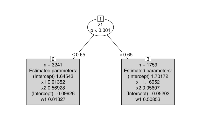
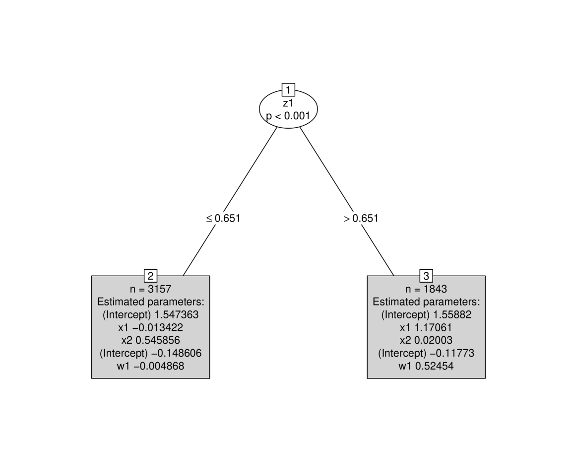
The estimated model for one of the simulated datasets with is shown in Figure 1. The results include the smooth terms for both and models and the tree.

The usefulness of the change-point estimation procedure is shown in Figure 2. When the data contains a clearly defined split-point, as in this case, it is identified by the maximum or one of the change-point statistics (in this case GLR test) calculated for each score function. It is evident from Figure 2 that the true split-point is identified by the GLR test statistics for each score function except for the score function for . Even in that case, the top 5% or 10% of the test statistics contain the true split-point.
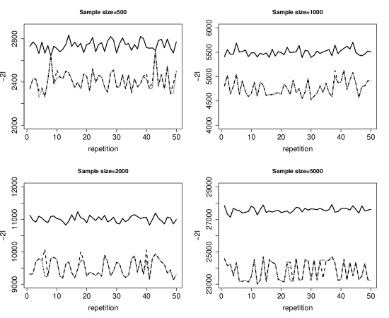
The full simulation results are described in Table 1. The results using the exhaustive search and the search with 10% change-points are identical except for one dataset with sample size . We find that the cut-off of 10% is mostly unnecessary as the cut-off of 5% suffices. While the results are slightly different for the models estimated with the exact set of change-points and the set of 10% change-points, in terms of the overall fit measures (local ), they are nearly identical. The computational times for the three models across all the simulated datasets are shown in Figure 3. Not surprisingly, the models based on change-point estimation methods are much faster compared to those based on exhaustive search, although the latter were made faster by using only one iteration from the IRLS for each potential split-point.


| Exhaustive Search | ||||
|---|---|---|---|---|
| Split-1 | ||||
| Global | ||||
| Local | ||||
| No.of terminal nodes | ||||
| Search with Exact Change-Points | ||||
|---|---|---|---|---|
| Split-1 | ||||
| Global | ||||
| Local | ||||
| No.of terminal nodes | ||||
| Search with 10% Change-Points | ||||
|---|---|---|---|---|
| Split-1 | ||||
| Global | ||||
| Local | ||||
| No.of terminal nodes | ||||
The results from Table 1 and Figure 3 indicate that when there exists a clear split-point in the data, as in the case of the simulated datasets, change-point estimation methods are useful for reducing the computational complexity. Moreover, differences from split-points estimated with the exact set of change-points do not necessarily imply estimation error, and in some cases those split-points make better sense practically, when interpreting the results. In practice, we suggest to first fit the model using the exact set of change-points and only then proceeding with the top 10% change-points or the exhaustive search method.
Appendix A2 provides a similar simulation, but where the moderator variables for and models are different. The results and conclusions are similar to those from the above example with the same moderators. When the moderator variables for and models were different, we noticed that the CMPMOB generated 3 to 4 partitions to accommodate those different splits. This is one of the limitations of CMPMOB, which is due to the dependence of the and models. More specifically, both models are estimated using the same data at each terminal node and they are not expected to have different estimated splits. In the next section, we propose a generalized model that overcomes this limitation and provides smoother approximations to the coefficient functions.
4 CMPBoost Semi-Varying Coefficient Model
4.1 Background
The CMPMOB model usually produces discontinuous and piece-wise approximations to the coefficient functions or . Gradient boosting (Freund & Schapire, 1996, 1997; Friedman, 2001) is a popular method that can provide more smoother estimates than a single tree. Gradient boosting is a recursive nonparametric algorithm with successful applications in many areas. The key idea is to combine a large number of base learners (such as simple trees) to achieve better predictive accuracy. For a comprehensive overview, see Friedman (2001) and Bühlmann (2006).
Recently, Wang & Hastie (2014) proposed a gradient boosting approach for the tree-based varying coefficient model. Our approach follows along the same lines but is more involved due to the complicated nature of the CMP distribution. We first briefly describe the approach proposed by Wang & Hastie (2014) and then propose our approach for the CMPBoost semi-varying coefficient model.
Consider the varying coefficient model: . By choosing an empirical loss function such as least square error or absolute error loss, the model can be estimated as follows:
| (19) |
where is the constrained function space. In boosting, the goal is to find an incremental model that minimizes empirical risk,
where is the model fit from the th iteration. The gradient boosting algorithm starts with a simple fit and then iteratively updates the estimate by adding the incremental model fitted on “residuals”, obtained by evaluating the negative gradient at the current fitted tree . The final boosting model has the following form:
| (20) |
with denoting the terminal node for the tree produced in the th boosting iteration and denotes the number of boosting steps. According to Wang & Hastie (2014), the boosting algorithm involves four tuning parameters: the number of boosting iterations , the learning rate , the minimal node size, and the size of each base learner . Based on Friedman (2001), one can use small values for , for example , to achieve better predictive accuracy.
The gradient boosting algorithm can be generalized to nonlinear and generalized linear models using different loss functions such as absolute error loss, Huber-loss (Bühlmann & Hothorn, 2007), or likelihood. In standard generalized linear models, the mean is related to the covariate function through a link function. Owing to this, one could follow the same approach as above to implement the gradient boosting algorithm when there is only one parameter. However, when there is a nuisance parameter in the likelihood, one possible option is to use the gradient boosting algorithm for the main parameter and later estimate the nuisance parameter directly. For example, Yang et al. (2018) provided the gradient boosting algorithm for Tweedie compound Poisson models. The authors first fix the nuisance parameter and estimate the mean parameter through gradient boosting. Once the mean parameter is estimated, they use the profile likelihood approach to estimate the nuisance parameter. While this approach works for the Tweedie compound Poisson distribution, it might not be appropriate for the CMP distribution because it is not possible to fix the parameter and estimate the parameter (or parameter in Huang (2017)) separately. For this reason, we consider updating both parameters in the gradient boosting algorithm.
4.2 CMPBoost Estimation
We propose an estimation procedure for the CMPBoost model using regression trees as base learners. Similar to the IRLS algorithm for estimating CMP regression (see Section 2), our proposed approach updates both the parameters and . For this two-step estimation, we consider the following model formulation that is even more flexible than the one in (7, 8)
| (21) | |||
| (22) |
where is another set of moderator variables. In practice, the moderator variables in both the models, and , can be the same or completely different. Note that the model formulation for the CMPMOB tree uses the same set of moderators for both (7) and (8) as both parameters need to be estimated at each terminal node using the same data. For this reason, CMPMOB tree is limited in the sense that it does not support formulation (21) and (22). On the other hand, the CMPBoost model is flexible enough to allow different moderators for each of (21) and (22), although model interpretation becomes more complicated.
Using the notation from Section 2, the adjusted dependent variable for the model in (21) for the th iteration is expressed as
where and are the estimated mean and variance for the th iteration. The linear predictor is . As in the gradient boosting approach, the linear predictor is updated using the base learners fitted with the estimated residual as the dependent variable.
Similarly, the adjusted dependent variable for the model in (22) for the th iteration is expressed as:
where and are the estimated mean and variance for in the th iteration. If the model also contains varying coefficients, the same approach is used to update the linear predictor . The base learners are fitted to the estimated residual for updating the linear predictor similar to (20).
Since the estimated residual is a continuous variable, any regression tree algorithm can be used to fit the base learner. We consider the “PartReg” algorithm (Wang & Hastie, 2014) as it is easy to control its tuning parameters and simpler to evaluate its model predictions. For example, it is not straightforward to apriori limit the number of terminal nodes in a MOB tree, since the algorithm first grows a larger-than-necessary tree and then prunes it back to the desired size. In contrast, limiting the number of terminal nodes is easy with the PartReg algorithm as it uses breadth-first search cycles. The PartReg algorithm does have some drawbacks, such as its selection bias towards variables with many split points (Strobl et al., 2008) and computational challenges for identifying split points in ordinal and nominal variables (see Wang & Hastie (2014) for a detailed discussion). Nonetheless, we still consider the PartReg algorithm as it is convenient, and we leave the MOB algorithm implementation of the CMPBoost model for future work.
The boosting algorithm has four tuning parameters, namely, , , and the minimal node size. Among these four, we fix , , or , and the minimal node size as in our simulation studies and real examples. The number of boosting iterations depends on the value chosen for ; a smaller value leads to more iterations. The choice of both and is data-dependent.111Care should be taken while setting the value for , as large values can sometimes lead to non-convergence of the algorithm. It is therefore advisable to first experiment with a few values and observe the convergence path (sequence of values) and number of iterations. We use the log likelihood evaluation criterion and stop the algorithm when there is not much improvement in the evaluation criterion, and hence is determined automatically. If a very small value is chosen for the parameter , we usually set to a fixed number, say . Finally, the parameter , the number of terminal nodes, is evaluated based on the performance on the test data.
As mentioned, one of the major limitations of the CMPMOB model is its computational complexity. However, the proposed CMPBoost model is computationally simpler than the CMPMOB, as the base learners are regular regression trees which are faster to compute. To interpret the results from CMPBoost, one can use variable importance plots and partial dependence plots as suggested by Wang & Hastie (2014). Following Friedman (2001) and Hastie et al. (2015), the importance of variable in a single tree is defined as
where denotes the variable chosen for splitting in the th step, is the number of terminal nodes, and is the improvement in the th iteration of the model fit. In boosting, we denote the th tree as and compute the relative importance of as the average of among all iterations, namely,
Coefficient interpretation has always been tricky with CMP models. Furthermore, it is also not easy to construct partial dependence plots for the proposed CMPBoost due to the two models, , , which are not orthogonal and their updates depend on each other. We illustrate some of these issues in a simulation study in the following section.
4.3 Simulation Study 2: CMPBoost
The goal of this simulation study is to showcase the flexibility of CMPBoost. We examine a case that includes varying coefficients for both intercept and slope terms in the and models with different moderator variables.
The simulation design is as follows:
-
•
Generate and , where , .
-
•
Compute the intercept functions , and the slope functions , .
-
•
Generate the dependent variable .
To allow sparsity, we let the true functions and only depend on the moderator variables and . Similarly, the true functions and depend on and , respectively. The total sample size is , and we leave 40% of the observations for the test data while the remaining 60% is used as training data. The tuning parameter , the number of terminal nodes for each base learner, is determined based on the out-of-sample prediction error (or ). In general, the algorithm iterates until there is not much change in the value or for a predefined number of iterations, , and hence is determined automatically. The minimum node size is chosen as and the learning parameter is set as .
Figure 4 shows the results for the models fitted with an increasing number of terminal nodes for base learners () on both training and test data. Both and prediction error have similar behavior and obtain their minimum at on the test data.222To remove possible overfitting associated with the number of boosting iterations, for each we let the model fitted to the training data run until there is not much change in , and we fix the same number of iterations for the model on the test data for that specific . For example, if the model with takes iteration for the training data, the same iterations are used to evaluate the prediction error on the test data.

We simulated 20 data sets with sample size and constructed the partial dependence plots. Interpreting the coefficient functions from the CMP model is not straightforward. As discussed in Section 2, the coefficients for the model depends on the parameter and are approximately scaled down by in terms of the mean parameter. Nevertheless, we constructed the partial dependence plots, for each varying coefficient function, analogous to the approach used by Wang & Hastie (2014).
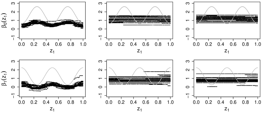
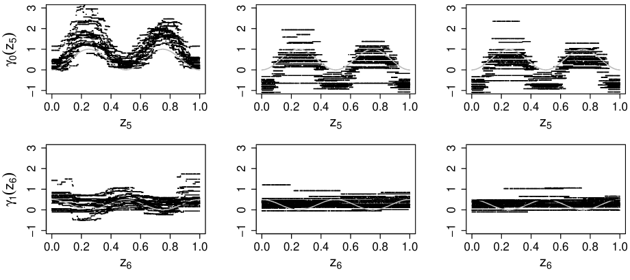
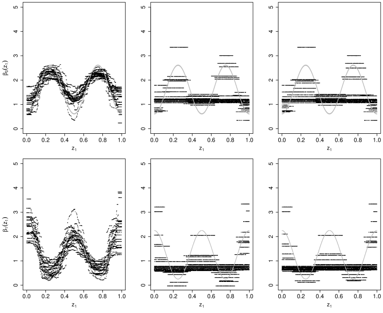
Figure 6 plots the true and estimated partial functions for both intercept and slope varying coefficients of the model, namely, where is the vector of averages of all the moderator variables except . We compared three methods: CMPBoost, CMPMOB with split points estimated via exhaustive search, and CMPMOB with split points estimated via 10% change points. The results illustrate that CMPBoost is able to reconstruct the underlying smooth function whereas CMPMOB provides only a piece-wise constant approximation. This is a key advantage of using the CMPBoost model. Further, it is computationally much simpler because of the base learner trees that are fitted using ordinary linear regression trees (for a continuous variable) which are less computationally expensive. Similarly, Figure 6 plots the true and estimated partial functions for both the intercept and slope varying coefficients of the model, namely, . From the results in both figures, we see that all three methods under-estimated the model and over-estimated the model. The reason is that the algorithms have terminated early due to the non-smooth objective function surface. The complicated nature of the simulated data can be attributed to this finding. This was verified by conducting a less complicated simulation design that considers a linear function with no varying coefficient terms for the model, in which case the proposed methods estimated the true functions without any problems (see Appendix A3).
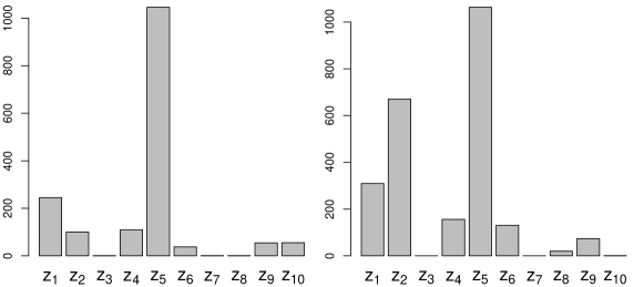
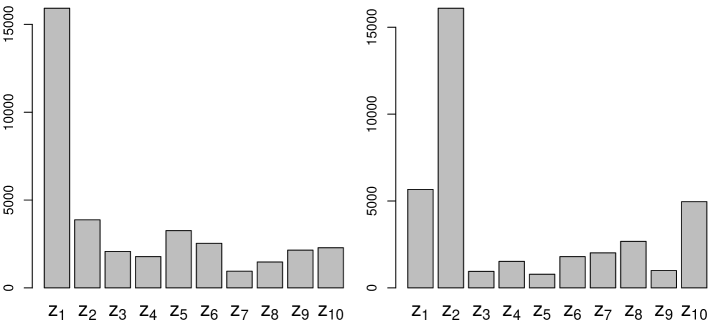
The variable importance plots for two specific datasets among the 20 simulated datasets are described in Figure 7. Although 4 true moderator variables were used to simulate the data, most of the time the moderator variables and dominated the other moderator variables. This occurs even for the CMPMOB models. Hence, the variable importance plots are correctly identifying the dominating moderators.
On the whole, the results from this example reiterate the fact that CMPBoost is a more flexible and robust approach than CMPMOB. In the following section, we apply and compare CMPMOB and CMPBoost on a real data example.
5 Modeling Data from a Bike Sharing System
We use CMPMOB and CMPBoost to analyze data from a bike sharing system. Bike sharing systems are the new generation bike rental service providers. The data come from a bike sharing service provider in Washington DC (Fanaee-T & Gama, 2014). For simplicity, we consider only data for January, 2012. It includes information on the number of hourly rentals for registered and casual users, the weather, whether or not the day is a holiday, etc. Table 2 provides the list of attributes and their descriptions. Descriptive statistics for the data are reported in Table A2 in Appendix A4. There are three missing values in the data and for that reason it included only 741 observations instead of 744 () observations. In this study, we model only the casual users; the same analysis can be repeated for the registered users.
| Name | Description |
|---|---|
| dteday | date |
| season | season (1:spring, 2:summer, 3:fall, 4:winter) |
| yr | year (0: 2011, 1:2012) |
| mnth | month ( 1 to 12) |
| hr | hour (0 to 23) |
| day | day (1 to 30 or 31) |
| holiday | whether or not the day is a holiday (extracted from |
| http://dchr.dc.gov/page/holiday-schedule) | |
| weekday | day of the week |
| workingday | if day is neither weekend nor holiday is 1, otherwise is 0. |
| weathersit | 1= Clear, Few clouds, Partly cloudy |
| 2= Mist + Cloudy, Mist + Broken clouds, Mist + Few clouds, Mist | |
| 3= Light Snow, Light Rain + Thunderstorm + Scattered clouds | |
| 4= Heavy Rain + Ice Pallets + Thunderstorm + Mist, Snow + Fog | |
| temp | Normalized temperature in Celsius. The values are divided to 41 (max) |
| atemp | Normalized feeling temperature in Celsius. The values are divided to 50 (max) |
| hum | Normalized humidity. The values are divided to 100 (max) |
| windspeed | Normalized wind speed. The values are divided to 67 (max) |
| casual | count of casual users |
| registered | count of registered users |
| cnt | count of total rental bikes including both casual and registered |
As a preliminary benchmark, we fit ordinary generalized linear models using both CMP and Poisson regressions (see Table A3 in Appendix A4). The CMP regression results in a large negative estimate for , indicating strong over-dispersion. The CMP and Poisson models diverge especially for variables hum and windspeed, which are highly significant in the Poisson but not in the CMP model. Not surprisingly, the CMP fit is much better in terms of AIC and log-likelihood.
5.1 Generalized Varying Coefficient Model
Now, we consider the following varying coefficient model:
| (23) | ||||
where and are four-dimensional functions.
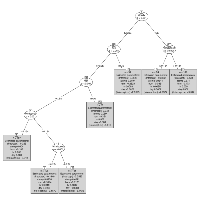
Binary coding is employed for the categorical variables (weathersit, weekday, holiday). The tree for the estimated CMPMOB with exhaustive search is shown in Figure 8. The tree identified cloudy, windspeed, sun and mon as significant. The exact same tree is obtained for CMPMOB model with the 10% change point method. The results indicate that ridership patterns are different for cloudy vs. non cloudy days and on weekdays vs. weekends. This is meaningful because weather and holidays play a significant role. Another important finding is that, although windspeed is not significant in the CMP regression model as a main effect, it is significant as a moderator in the CMPMOB tree.
The estimated Poisson MOB (Figure A6 in Appendix A4) identified sat and sun as significant moderators. Surprisingly, windspeed which is selected as a main effect in the Poisson regression is not included in the tree. This might be due to the inability of the Poisson distribution to capture over-dispersion.
To assess the variable importance and to provide smoother approximations for Model (23), we fitted the CMPBoost model. The tuning parameter for minimum node size is chosen as 20, and is chosen to reduce the number of boosting iterations , which is determined automatically. For the number of terminal nodes , we used a test data (January, 2011) to find the optimal value . With these tuning parameters, the CMPBoost took iterations. The variable importance plot is shown in Figure 9. Similar to the CMPMOB tree, the CMPBoost identified windspeed as the most significant. Apart from that, sat, lightrain and notholiday have high importance scores. Surprisingly, cloudy, which is selected as a significant variable in the CMPMOB Tree in Figure 8, has a low variable importance score. This could be attributed to the instability problem of a single tree.

To gain further insight into the results from the CMPBoost model, partial dependence plots for windspeed are constructed (Figure 10). Similar plots can be constructed for other significant moderator variables such as sat, notholiday or lightrain. Figure 10 shows that for moderate wind speed, atemp seems to have a positive effect on ridership. Similarly, hum seems to have an overall negative effect on ridership except for a few moderate wind speed values. In contrast, hr has a positive relationship with ridership except for a few moderate values of wind speed. It is surprising to see that the partial dependence plots in Figure 10 are not smooth as expected in the CMPBoost model. This may be due to the presence of categorical variables in the functions in (23) that make the underlying true function itself not smooth.

5.2 A More Flexible Generalized Semi-Varying Coefficient Model
To provide even more flexibility, we consider the following semi-varying coefficient model:
| (24) | ||||
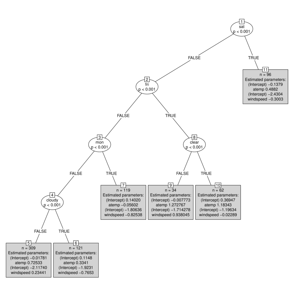
where and functions , are global, and are not re-estimated at each node of the tree or in the boosting algorithm. The tree for the CMPMOB (Figure A8 in Appendix A4) selected the variables sat, fri, mon, clear and cloudy as significant moderators. The variable atemp has a positive effect on ridership except on Mondays, when the effect seems to be negative. Similarly, windspeed seems to create more variation in ridership on Fridays, Saturdays and Mondays if the weather is clear, and also on the remaining days if the weather is cloudy. The global smooth functions are presented in Figure 11, showing that rentals follow a cyclical pattern across days, which could be due to a weekend/weekday effect. Further, rentals are highest in the afternoon compared to evenings or early mornings.

The CMPBoost model is fitted using the same tuning parameters as in the previous model. The overall likelihood value () is slightly better than the CMPMOB tree. Comparing the CMPMOB tree (Figure A8 in Appendix A4) and the variable importance measures of the CMPBoost (Figure A7 in Appendix A4), in both cases fri and sat are the most influential variables. More importantly, the model selected fri as the most influential moderator whereas the model selected the variable sat. Based on this finding, we constructed the partial dependence plots for the coefficient functions , with respect to fri, and for the functions , with respect to sat. The results are shown in Figure 12.

To conclude, the results show that both the CMPBoost and CMPMOB are very flexible for modeling the bike sharing data and they provide valuable insights.
6 Summary and Conclusions
We proposed a novel tree-based semi-varying coefficient model for the CMP distribution. Our CMPMOB model formulation is more flexible than existing tree-based models for count data, as it allows including node-invariant (global) effects in the model. A known drawback of tree-based methods is that they only provide a piece-wise constant approximation to the underlying smooth functions. To overcome this limitation, we also developed a boosting approach, CMPBoost, to provide smoother estimates of the underlying varying coefficient functions. We provide R code for all of these procedures at https://github.com/SuneelChatla/CMPTree.
We used the MOB algorithm to estimate the proposed tree-based semi-varying coefficient model because it provides coefficient-constancy tests that are easy to implement. The methodology can be extended to any tree-based estimation approach, such as PartReg. The existing MOB algorithm uses exhaustive search to identify potential split points and is computationally intensive for the CMP distribution. We provided some heuristics to reduce the computational burden and at the same time, we proposed a new split point estimation approach by borrowing tools from the change-point estimation literature.
On the whole, the proposed semi-varying coefficient models (CMPBoost and CMPMOB) are shown to be useful for handling count data. In addition to their ability to capture both over- and under-dispersion, their flexibility to model complex nonlinear relationships makes them powerful tools for analyzing count data in a wide range of applications.
References
- (1)
- Antoch et al. (1995) Antoch, J., Hušková, M. & Veraverbeke, N. (1995), ‘Change-point problem and bootstrap’, Journal of Nonparametric Statistics 5(2), 123–144.
- Banerjee & McKeague (2007) Banerjee, M. & McKeague, I. W. (2007), ‘Confidence sets for split points in decision trees’, The Annals of Statistics 35(2), 543–574.
- Boukai (1993) Boukai, B. (1993), ‘A nonparametric bootstrapped estimate of the change-point’, Journal of Nonparametric Statistics 3(2), 123–134.
- Breiman & Friedman (1985) Breiman, L. & Friedman, J. H. (1985), ‘Estimating optimal transformations for multiple regression and correlation’, Journal of the American statistical Association 80(391), 580–598.
- Brodsky & Darkhovsky (2013) Brodsky, E. & Darkhovsky, B. S. (2013), Nonparametric Methods in Change point Problems, Vol. 243, Springer Science & Business Media.
- Bühlmann (2006) Bühlmann, P. (2006), ‘Boosting for high-dimensional linear models’, The Annals of Statistics 34(2), 559–583.
- Bühlmann & Hothorn (2007) Bühlmann, P. & Hothorn, T. (2007), ‘Boosting algorithms: Regularization, prediction and model fitting’, Statistical Science 22(4), 477–505.
- Bürgin & Ritschard (2015) Bürgin, R. & Ritschard, G. (2015), ‘Tree-based varying coefficient regression for longitudinal ordinal responses’, Computational Statistics & Data Analysis 86, 65–80.
- Chan & Loh (2004) Chan, K.-Y. & Loh, W.-Y. (2004), ‘Lotus: An algorithm for building accurate and comprehensible logistic regression trees’, Journal of Computational and Graphical Statistics 13(4), 826–852.
- Chatla & Shmueli (2018) Chatla, S. B. & Shmueli, G. (2018), ‘Efficient estimation of COM-Poisson regression and additive model’, Computational Statistics and Data Analysis 121, 71–88.
- Fan & Zhang (2000) Fan, J. & Zhang, W. (2000), ‘Simultaneous confidence bands and hypothesis testing in varying-coefficient models’, Scandinavian Journal of Statistics 27(4), 715–731.
- Fan & Zhang (2008) Fan, J. & Zhang, W. (2008), ‘Statistical methods with varying coefficient models’, Statistics and its Interface 1(1), 179.
- Fanaee-T & Gama (2014) Fanaee-T, H. & Gama, J. (2014), ‘Event labeling combining ensemble detectors and background knowledge’, Progress in Artificial Intelligence 2(2-3), 113–127.
-
Freund & Schapire (1996)
Freund, Y. & Schapire, R. E. (1996), Experiments with a new boosting algorithm, in ‘Proceedings of the
Thirteenth International Conference on International Conference on Machine
Learning’, ICML’96, Morgan Kaufmann Publishers Inc., San Francisco, CA, USA,
pp. 148–156.
http://dl.acm.org/citation.cfm?id=3091696.3091715 - Freund & Schapire (1997) Freund, Y. & Schapire, R. E. (1997), ‘A decision-theoretic generalization of on-line learning and an application to boosting’, Journal of Computer and System Sciences 55(1), 119–139.
- Friedman (2001) Friedman, J. H. (2001), ‘Greedy function approximation: A gradient boosting machine’, Annals of Statistics 29(5), 1189–1232.
- Hastie & Tibshirani (1993) Hastie, T. & Tibshirani, R. (1993), ‘Varying-coefficient models’, Journal of the Royal Statistical Society. Series B (Methodological) 55(4), 757–796.
- Hastie et al. (2015) Hastie, T., Tibshirani, R. & Wainwright, M. (2015), Statistical Learning with Sparsity: The Lasso and Generalizations, Chapman & Hall/CRC.
- Hawkins & Zamba (2005) Hawkins, D. M. & Zamba, K. (2005), ‘A change-point model for a shift in variance’, Journal of Quality Technology 37(1), 21.
- Hinkley (1970) Hinkley, D. V. (1970), ‘Inference about the change-point in a sequence of random variables’, Biometrika 57(1), 1–17.
- Hothorn & Zeileis (2013) Hothorn, T. & Zeileis, A. (2013), ‘Partykit: A toolkit for recursive partytioning, 2013’, R package version 0.1-6 66.
- Huang (2017) Huang, A. (2017), ‘Mean-parametrized conway–maxwell–poisson regression models for dispersed counts’, Statistical Modelling 17(6), 359–380.
- Kaufman (2018) Kaufman, R. L. (2018), Interaction Effects in Linear and Generalized Linear Models: Examples and Applications Using Stata, Vol. 12, SAGE Publications.
- Kim & Loh (2001) Kim, H. & Loh, W.-Y. (2001), ‘Classification trees with unbiased multiway splits’, Journal of the American Statistical Association 96(454), 589–604.
- Loh (2002) Loh, W.-Y. (2002), ‘Regression trees with unbiased variable selection and interaction detection’, Statistica Sinica 12, 361–386.
- Loh & Shih (1997) Loh, W.-Y. & Shih, Y.-S. (1997), ‘Split selection methods for classification trees’, Statistica Sinica 7, 815–840.
- Park et al. (2015) Park, B. U., Mammen, E., Lee, Y. K. & Lee, E. R. (2015), ‘Varying coefficient regression models: A review and new developments’, International Statistical Review 83(1), 36–64.
-
Ross (2015)
Ross, G. (2015), ‘Parametric and
nonparametric sequential change detection in r: The cpm package’, Journal of Statistical Software, Articles 66(3), 1–20.
https://www.jstatsoft.org/v066/i03 - Sellers & Shmueli (2010) Sellers, K. F. & Shmueli, G. (2010), ‘A flexible regression model for count data’, Annals of Applied Statistics 4(2), 943–961.
- Sellers & Shmueli (2013) Sellers, K. F. & Shmueli, G. (2013), ‘Data dispersion: Now you see it– now you don’t’, Communications in Statistics-Theory and Methods 42(17), 3134–3147.
- Shmueli et al. (2005) Shmueli, G., Minka, T. P., Kadane, J. B., Borle, S. & Boatwright, P. (2005), ‘A useful distribution for fitting discrete data: Revival of the Conway-Maxwell-Poisson distribution’, Journal of the Royal Statistical Society: Series C (Applied Statistics) 54(1), 127–142.
- Strobl et al. (2008) Strobl, C., Boulesteix, A.-L., Kneib, T., Augustin, T. & Zeileis, A. (2008), ‘Conditional variable importance for random forests’, BMC Bioinformatics 9(1), 307.
- Wang & Hastie (2014) Wang, J. C. & Hastie, T. (2014), ‘Boosted varying-coefficient regression models for product demand prediction’, Journal of Computational and Graphical Statistics 23(2), 361–382.
-
Wood (2017)
Wood, S. N. (2017), ‘mgcv’, R Package
Version 1.8-18 .
https://CRAN.R-project.org/package=mgcv - Xia et al. (2004) Xia, Y., Zhang, W. & Tong, H. (2004), ‘Efficient estimation for semivarying-coefficient models’, Biometrika 91(3), 661–681.
- Yang et al. (2018) Yang, Y., Qian, W. & Zou, H. (2018), ‘Insurance premium prediction via gradient tree-boosted tweedie compound poisson models’, Journal of Business & Economic Statistics 36(3), 456–470.
- Zeileis (2005) Zeileis, A. (2005), ‘A unified approach to structural change tests based on ml scores, f statistics, and ols residuals’, Econometric Reviews 24(4), 445–466.
- Zeileis et al. (2008) Zeileis, A., Hothorn, T. & Hornik, K. (2008), ‘Model-based recursive partitioning’, Journal of Computational and Graphical Statistics 17(2), 492–514.
- Zhang et al. (2002) Zhang, W., Lee, S.-Y. & Song, X. (2002), ‘Local polynomial fitting in semivarying coefficient model’, Journal of Multivariate Analysis 82(1), 166–188.
A1 Appendix A1: CMPMOB Algorithm
The algorithm for CMPMOB semi-varying coefficient model is given below. First, it fits a global model with all the terms in the model including fixed effects terms using all the data. Once the fixed/global effects are estimated, the MOB procedure starts by constructing a tree with the splitting variables. The estimated fixed effects values will be treated as offset terms in all the subsequent models. After the tree is fitted, the fixed/global effects are re-estimated using the tree model as an offset term.
A2 Appendix A2: CMPMOB Simulation with Different Split Variables for the model
The simulation design for this example is same as for the example in Section 3.3 except that both and use different split variables and split points. More specifically, we now consider with and with . The remaining details are same as in Section 3.3.
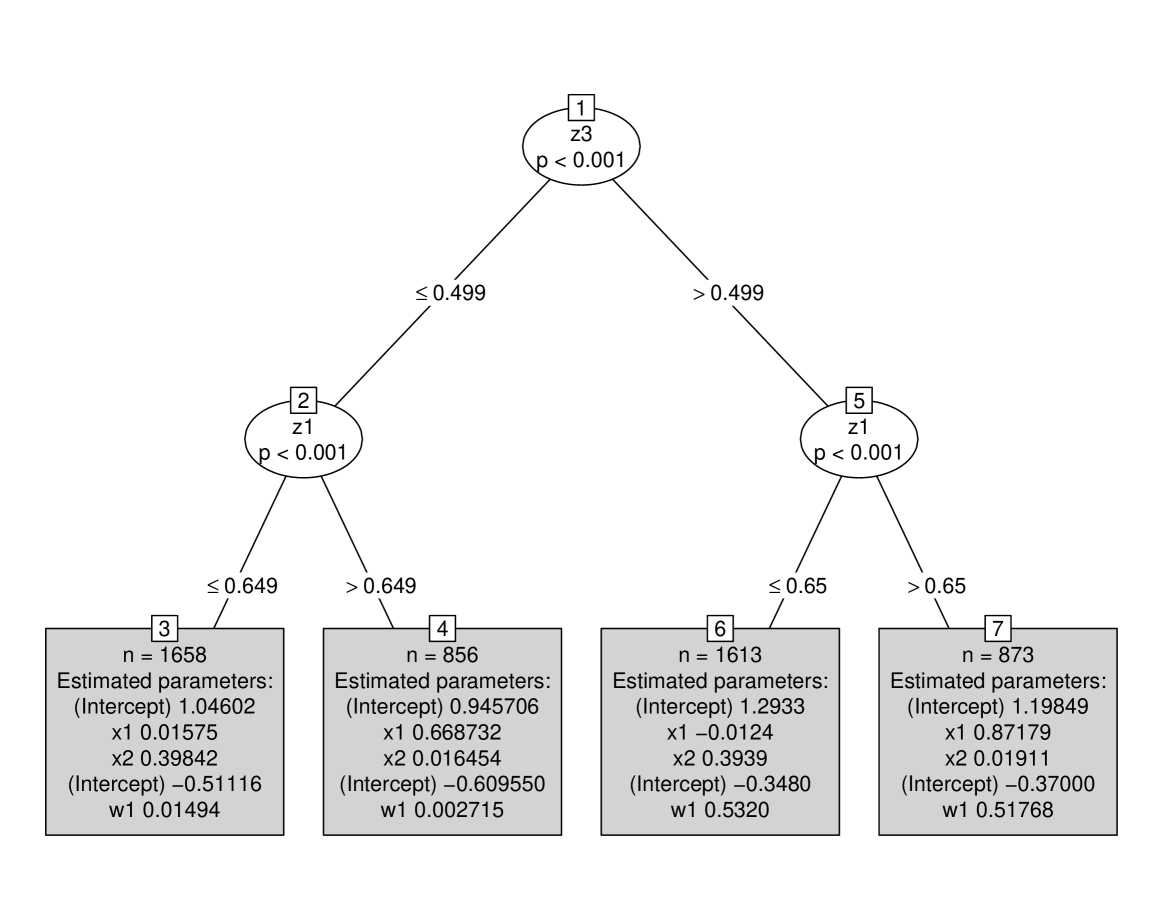
The estimated tree for one of the data sets is shown in Figure A1. This time, the first tree chose 4 terminal nodes to accommodate the two true underlying splits. The estimated splits are . On the other hand, the second tree has only 3 terminal nodes in which the variable is probably not significant under . Obviously, the fit measure for the first tree (rep 1) is much better than the second tree (rep 20) which is evident from the right bottom plot in Figure A2. Note that both and must be estimated simultaneously using the same data and hence they cannot have different splits at the same time. This is the reason why we considered the same splitting variables in both (7) and (8).
The findings from this example are consistent with the findings in Section 4.3. As shown in Figure A2 and Table A1, the results from 10% change points are identical to the results from exhaustive search except for the data sets with . Even in that case, the results are not practically different as their overall fit measures are very close. The results from the model estimated using the exact set of change points are also very close to the results from the model estimated using exhaustive search, both in terms of overall fit and the estimated split points.
| Exhaustive Search | ||||
|---|---|---|---|---|
| Split-1 | ||||
| Split-2 | ||||
| Split-3 | ||||
| Split-4 | ||||
| Global | ||||
| Local | ||||
| Search with Exact Change Points | ||||
|---|---|---|---|---|
| Split-1 | ||||
| Split-2 | ||||
| Split-3 | ||||
| Global | ||||
| Local | ||||
| Search with 10% Change Points | ||||
|---|---|---|---|---|
| Split-1 | ||||
| Split-2 | ||||
| Split-3 | ||||
| Split-4 | ||||
| Global | ||||
| Local | ||||
A3 Appendix A3: CMPBoost Simulation with Linear Function (no varying coefficient terms) for
The simulation design is exactly as described in Section 4.3 except that we do not use varying coefficients for the model, but rather a linear function of the form .
Figure A3 shows the results for the models fitted with an increasing number of terminal nodes for base learners () on both training and test data. Both and prediction error have similar behavior and obtain their minimum at on the test data.

Figure A4 plots the true and estimated partial functions for both intercept and slope varying coefficients where is the vector of averages of all the moderator variables except . As in Section 4.3, we compared three methods: CMPBoost, CMPMOB with split points estimated via exhaustive search, and CMPMOB with split points estimated via 10% change points. And similarly to the varying coefficients example in Section 4.3, the results here illustrate that CMPBoost is able to reconstruct the underlying smooth function whereas CMPMOB provides only a piece-wise constant approximation.
Based on the results obtained from the CMPBoost model, we also constructed the variable importance plot for the moderator variables (Figure A5). As expected, both and are the only significant moderator variables. For the majority of the datasets (out of 20 simulations), the variable importance measure is higher for moderator variable although both and are used in the simulation. For a few simulations, the variable importance measure is higher for . This might be a result of sampling variation.
On the whole, these results reiterate the fact that CMPBoost is a more flexible and robust approach than CMPMOB.
A4 Appendix A4: Bike Sharing Analysis - Comparison with Poisson and CMP GLM
| Statistic | N | Mean | St. Dev. | Min | Pctl(25) | Pctl(75) | Max |
|---|---|---|---|---|---|---|---|
| holiday | 741 | 0.063 | 0.244 | 0 | 0 | 0 | 1 |
| weekday | 741 | 2.811 | 2.011 | 0 | 1 | 5 | 6 |
| workingday | 741 | 0.645 | 0.479 | 0 | 0 | 1 | 1 |
| temp | 741 | 0.275 | 0.103 | 0.020 | 0.200 | 0.340 | 0.580 |
| atemp | 741 | 0.275 | 0.101 | 0.015 | 0.212 | 0.333 | 0.546 |
| hum | 741 | 0.587 | 0.203 | 0.210 | 0.420 | 0.760 | 1.000 |
| windspeed | 741 | 0.217 | 0.130 | 0 | 0.1 | 0.3 | 1 |
| casual | 741 | 12.104 | 19.478 | 0 | 1 | 14 | 156 |
| registered | 741 | 118.455 | 109.922 | 1 | 29 | 168 | 518 |
| cnt | 741 | 130.559 | 119.797 | 1 | 32 | 191 | 559 |
This appendix contains results that supplement Section 5. Table A3 contains the results from both Poisson and CMP generalized linear models. Not surprisingly, the CMP GLM performed better in terms of overall fit. In addition, Poisson regression, which is not flexible enough to model the data over dispersion, identifies hum and windspeed as significant while the CMP GLM does not. Since the MOB framework uses coefficient constancy tests, it is possible that the limitations of Poisson regression are carried over to the Poisson MOB tree. For this reason, the Poisson MOB tree in Figure A6 looks completely different from the CMPMOB tree in Figure 8.
| Poisson GLM | CMP GLM | |
| day | 0.007∗∗∗ (0.001) | 0.001∗∗∗ (0.001) |
| hr | 0.026∗∗∗ (0.002) | 0.003∗∗∗ (0.001) |
| holiday: holiday | 0.629∗∗∗ (0.075) | 0.113∗∗ (0.034) |
| weekday: mon | 0.998∗∗∗ (0.058) | 0.138∗∗∗(0.028) |
| weekday: tue | 1.100∗∗∗ (0.040) | 0.126∗∗∗ (0.015) |
| weekday: wed | 0.641∗∗∗ (0.043) | 0.070∗∗∗ (0.017) |
| weekday: thu | 0.919∗∗∗ (0.044) | 0.103∗∗∗ (0.018) |
| weekday: fri | 1.021∗∗∗ (0.041) | 0.110∗∗∗ (0.016) |
| weekday: sat | 0.021 (0.031) | 0.019⋅ (0.010) |
| weathersit: cloudy | 0.165∗∗∗ (0.030) | 0.028∗ (0.011) |
| weathersit: light rain/fog | 0.844∗∗∗ (0.070) | 0.145∗∗∗(0.037) |
| weathersit: heavy rain/fog | 0.353 (0.380) | 0.101 (0.228) |
| atemp | 5.709∗∗∗ (0.114) | 0.617∗∗∗ (0.047) |
| hum | 0.595∗∗∗ (0.074) | 0.045 (0.029) |
| windspeed | 0.326∗∗∗ (0.096) | 0.010 (0.036) |
| Constant | 1.155∗∗∗ (0.069) | 0.108∗∗∗ (0.028) |
| 2.99∗∗∗ (0.022) | ||
| Observations | 741 | 741 |
| Log Likelihood | 4951.48 | 2417.20 |
| Akaike Inf. Crit. | 9934.96 | 4869.40 |
| ⋅p0.1; ∗p0.05; ∗∗p0.01 ; ∗∗∗p0.001 |
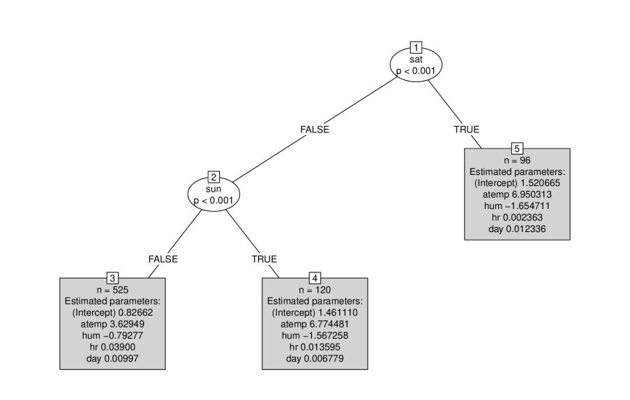
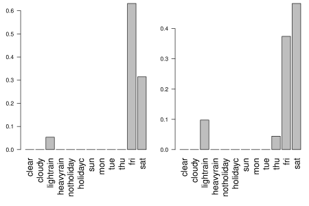
For the more flexible model in (24), the CMPMOB tree is given in Figure A8. Similar to the CMPMOB tree in Figure 8, it identified weather and weekday as the significant factors affecting demand after controlling for the other factors such as atemp and hum.
For the CMPBoost semi-varying coefficient model, the variable importance results for both the parameters are given in Figure A7. As mentioned in Section 5, while the model identified fri and sat as the top 2 variables, the model identified sat and fri as the top 2 variables. These results illustrate the flexibility of the CMPBoost semi-varying coefficient model.
