A Barometric Exponential Model of the Atmosphere’s Refractive Index: Zenith Angles and Second Order Aberration in the Entrance Pupil

Abstract

This report models the refractive index above a telescope site by an atmosphere with exponential decay of the refractive index (susceptibility) as a function of altitude. The air is represented as a spherical hull around the surface. We compute (i) the differential zenith angle — the difference between the actual zenith angle at arrival of rays at the telescope and a hypothetical zenith angle without the atmosphere — and (ii) the optical path length distribution of rays at arrival in the entrance pupil as a function of the distance to the pupil center.

The key technique in this work is to expand some integrals — that depend on the refractive index profile along the curved path of each ray from some virtual plane in the direction of the star up to the entrance pupil — in power series of small parameters.

I Spherical Symmetry of the Atmospheric Hull

In ground-based astronomy, light emitted by astronomical objects is tilted more toward the zenith axis when arriving at the telescope than computed by standard spherical astronomy; the atmosphere acts like a gradient lens, and the actual zenith angle of arrival $z_{0}$ differs from the astrometric zenith angle $z$ of a hypothetical Earth in vacuum by an angle

$$R=z-z_{0}.$$ (1)

Figure 1 sketches the relevant variables.

Figure 1: Distance $\rho$ of the telescope to the Earth center, distance $r$ of a point on the curved path of the ray, true zenith angle $z_{0}$, astrometric zenith angle $z$, and impact parameter $I$. (Not to scale.)

Applying successively Snell’s equations as light changes its direction when it encounters gradients in the refractive index $n$, the angle $R$ is a functional of the refractive index along the path Mahan (1962); Green (1985); Thomas and Joseph (1996); Auer and Standish (2000); Nener et al. (2003); Noerdlinger (1999); Tannous and Nigrin (2001)

$$R=\rho n_{0}\sin z_{0}\int_{1}^{n_{0}}\frac{dn}{n\sqrt{r^{2}n^{2}-\rho^{2}n_{0}^{2}\sin^{2}z_{0}}}$$ (2)

measured in radians. $\rho\approx 6378$ km is the radius of the Earth representing the curvature of the atmosphere above the telescope National Imagery and Mapping Agency (2000). $n(r)$ is the refractive index at a distance $r\geq\rho$ to the Earth center (!); it equals unity high above the atmosphere and increases to $n_{0}>1$ at the telescope’s altitude.

Evaluating $R$ is a key to faithful pointing models and all-sky mapping of astrometry. Inserting wavelength-dependent refractive indices $n$ leads to designs of atmospheric dispersion correctors.

We start from the Taylor expansion of $R$ in odd powers of the tangent of the observed zenith angle Stone (1996, 2002),

$$R\equiv\sum_{i=1,3,5,\ldots}\gamma_{i}\tan^{i}z_{0},$$ (3)

such that Mathar (2005)

$$\gamma_{1} = \rho n_{0}\int_{1}^{n_{0}}\frac{1}{n^{2}r}dn;$$ (4)

$$\gamma_{3} = \frac{1}{2}\rho n_{0}\int_{1}^{n_{0}}\frac{\rho^{2}n_{0}^{2}-r^{2}n^{2}}{n^{4}r^{3}}dn;$$ (5)

$$\gamma_{5} = \frac{3}{8}\rho n_{0}\int_{1}^{n_{0}}\frac{(\rho^{2}n_{0}^{2}-r^{2}n^{2})^{2}}{n^{6}r^{5}}dn;$$ (6)

$$\gamma_{i} = {{i-1}\choose{\lfloor i/2\rfloor}}\frac{1}{4^{\lfloor i/2\rfloor}}\rho n_{0}\int_{1}^{n_{0}}\frac{(\rho^{2}n_{0}^{2}-r^{2}n^{2})^{\lfloor i/2\rfloor}}{n^{i+1}r^{i}}dn,\quad i=1,3,5,\ldots\,\mathrm{odd},$$ (7)

where $\lfloor.\rfloor$ is the floor function, the largest integer not larger than the term inside the bracket.

II Exponential Refractivity of Altitude

The first theme of this manuscript is to derive manageable formulas for the coefficients $\gamma_{i}$ by introducing an exponential model of the refractive index $n(r)$ as a function of altitude Berberan-Santos et al. (1997); West (1996). The refractive index is related to the susceptibility $\chi$ via

$$n(r)=\sqrt{1+\chi(r)}$$ (8)

and we assume that the susceptibility is essentially proportional to an air density of scale height $K$ such that

$$\chi(r)=\chi_{0}e^{-(r-\rho)/K}.$$ (9)

[Note that this is not Fletcher’s model Fletcher (1931) which has another term proportional to $e^{-(r-\rho)/K}/(r-\rho)$.] At typical altitudes of observatories the susceptibility at the telescope is $\chi_{0}\approx 4\times 10^{-4}$, and the Earth atmosphere has a scale height $K\approx 9.6$ km.

With such an explicit refractive index profile, refractive indices are mapped onto dimensionless altitudes $\zeta\equiv(r-\rho)/K$:

$$\frac{dn}{d\zeta}=\frac{1}{2n}\frac{d\chi}{d\zeta},$$ (10)

$$\frac{d\chi}{d\zeta}=-\chi(\zeta),$$ (11)

and so the variables in the integrals of the previous chapter turn into:

$$\gamma_{1} = \rho n_{0}\int_{0}^{\infty}\frac{1}{n^{2}(\rho+\zeta K)}\frac{1}{2n}\chi(\zeta)d\zeta;$$ (12)

$$\gamma_{3} = \rho n_{0}\frac{1}{2}\int_{0}^{\infty}\frac{\rho^{2}n_{0}^{2}-r^{2}n^{2}}{n^{4}(\rho+\zeta K)^{3}}\frac{1}{2n}\chi(\zeta)d\zeta;$$ (13)

$$\gamma_{5} = \rho n_{0}\frac{3}{8}\int_{0}^{\infty}\frac{(\rho^{2}n_{0}^{2}-r^{2}n^{2})^{2}}{n^{6}(\rho+\zeta K)^{5}}\frac{1}{2n}\chi(\zeta)d\zeta.$$ (14)

The associated bivariate power series of $\gamma_{1}$ in terms of the small $\chi_{0}$ and $K/\rho$ is written down up to mixed third order in these two variables and integrated term-by-term:

$$\gamma_{1} = \rho n_{0}\frac{1}{2}\int_{0}^{\infty}\frac{1}{n^{3}(\rho+\zeta K)}\chi_{0}e^{-\zeta}d\zeta$$ (15)

$$= n_{0}\chi_{0}\frac{1}{2}\int_{0}^{\infty}\frac{1}{(1+\chi_{0}e^{-\zeta})^{3/2}(1+\zeta K/\rho)}e^{-\zeta}d\zeta$$

$$= n_{0}\chi_{0}\frac{1}{2}\int_{0}^{\infty}e^{-\zeta}\big{[}1-\frac{3}{2}e^{-\zeta}\chi_{0}-\zeta\frac{K}{\rho}+\frac{15}{8}e^{-2\zeta}\chi_{0}^{2}+\frac{3}{2}\zeta e^{-\zeta}\chi_{0}\frac{K}{\rho}+\zeta^{2}(\frac{K}{\rho})^{2}$$

$$+\frac{35}{16}e^{-3\zeta}\chi_{0}^{3}-\frac{15}{8}\zeta e^{-2\zeta}\chi_{0}^{2}\frac{K}{\rho}-\frac{3}{2}\zeta^{2}e^{-\zeta}\chi_{0}(\frac{K}{\rho})^{2}-\zeta^{3}(\frac{K}{\rho})^{3}\pm\cdots\big{]}d\zeta$$

$$= n_{0}\chi_{0}\frac{1}{2}\left[1-\frac{3}{4}\chi_{0}-\frac{K}{\rho}+\frac{5}{8}\chi_{0}^{2}+\frac{3}{8}\chi_{0}\frac{K}{\rho}+2(\frac{K}{\rho})^{2}-\frac{35}{64}\chi_{0}^{3}-\frac{5}{24}\chi_{0}^{2}\frac{K}{\rho}-\frac{3}{8}\chi_{0}(\frac{K}{\rho})^{2}-6(\frac{K}{\rho})^{3}\pm\cdots\right].$$

This kind of expansion as a power series of $K/\rho$ is not new Eshagh (2008).

• In practise $\chi_{0}$ is known not better than a relative accuracy of $10^{-4}$, and $K/\rho$ is of the same magnitude; so keeping more than the first 3 terms in the square bracket in that expansion is a mere academic exercise from the point of view of an error budget.

• If gas mixtures of the air are treated as independent linear responses such that $\chi_{0}$ is an additive composition proportional to the weighted contribution of the air components, this formula does obviously not apply beyond the first terms in the square bracket, because otherwise mixed quadratic terms of the individual $\chi_{0}$ of the constituents interfere with the higher orders (App. A).

• At a precision of better than a milli-arcsecond, the oblate ellipsoidal Earth model introduces two different principal curvatures $1/\rho$ here that induce an azimuthal wobble of the terms Mathar (2009).

For the third order in $\tan z_{0}$ up to second mixed order

$$\gamma_{3} = \rho n_{0}\frac{1}{4}\int_{0}^{\infty}\frac{\rho^{2}n_{0}^{2}-(\rho+\zeta K)^{2}n^{2}}{n^{5}(\rho+\zeta K)^{3}}\chi_{0}e^{-\zeta}d\zeta$$ (16)

$$= n_{0}\chi_{0}\frac{1}{4}\int_{0}^{\infty}\frac{n_{0}^{2}-(1+\zeta K/\rho)^{2}n^{2}}{(1+\chi_{0}e^{-\zeta})^{5/2}(1+\zeta K/\rho)^{3}}e^{-\zeta}d\zeta;$$

$$= n_{0}\chi_{0}\frac{1}{4}\left[\frac{1}{2}\chi_{0}-2\frac{K}{\rho}-\frac{5}{12}\chi_{0}^{2}-\frac{3}{2}\chi_{0}\frac{K}{\rho}+10(\frac{K}{\rho})^{2}\pm\cdots\right]$$

For the fifth order in $\tan z_{0}$ up to second mixed order

$$\gamma_{5} = \rho n_{0}\frac{3}{16}\int_{0}^{\infty}\frac{(\rho^{2}n_{0}^{2}-(\rho+\zeta K)^{2}n^{2})^{2}}{n^{7}(\rho+\zeta K)^{5}}\chi_{0}e^{-\zeta}d\zeta$$ (17)

$$= n_{0}\chi_{0}\frac{3}{16}\int_{0}^{\infty}\frac{(n_{0}^{2}-(1+\zeta K/\rho)^{2}n^{2})^{2}}{(1+\chi_{0}e^{-\zeta})^{7/2}(1+\zeta K/\rho)^{5}}e^{-\zeta}d\zeta$$

$$= n_{0}\chi_{0}\frac{3}{16}\left[\frac{1}{3}\chi_{0}^{2}-3\chi_{0}\frac{K}{\rho}+8(\frac{K}{\rho})^{2}\pm\cdots\right].$$

More $\gamma_{i}$ coefficients are in the function gamm() in the file RefrExpo.cxx in the source code (see App. C).

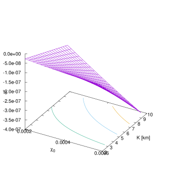
The difference between including only $\tan z_{0}$ and including all four terms up to $\tan^{7}z_{0}$ is for example 0.8 arcsec (112.60 arcsec versus 111.79 arcsec) for $z_{0}=70^{\circ}$ at $\chi_{0}=4\times 10^{-4}$ and $K/\rho=9.6/6380$. Then $\tan z_{0}=2.7$, and the dominating contribution to the 0.8 arcsec is the cube of 2.7 multiplied by the characteristic $\gamma_{3}\approx 40$ mas of Figure 3.

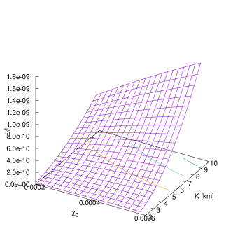
Figure 2: The coefficient $\gamma_{1}$ in radians as a function of $\chi_{0}$ and $K$ at $\rho=6380$ km. At this resolution there is almost no dependence on the scale height $K$, so $\gamma_{1}\approx n_{0}\chi_{0}/2$. $2\times 10^{-4}$ rad is equivalent to 41 arcsec at $z_{0}=45^{\circ}$.

Figure 3: The coefficient $\gamma_{3}$ in radians as a function of $\chi_{0}$ and $K$ at $\rho=6380$ km. $2\times 10^{-7}$ rad are equivalent to 40 mas at $z_{0}=45^{\circ}$.

Figure 4: The coefficient $\gamma_{5}$ in radians as a function of $\chi_{0}$ and $K$ at $\rho=6380$ km. $10^{-9}$ rad are equivalent to 0.2 mas at $z_{0}=45^{\circ}$.

III Active Optics Aberrations

The implication of the previous section for telescope operation is that the telescope axis is corrected by a tilt $R$ while acquiring an object at an astrometric zenith angle $z$. Which further imprint does the asymmetry of the global spherical atmosphere leave if the telescope’s primary mirror collects light from a beam which does not have a perfect cylindrical symmetry because the center of curvature of the atmosphere is not on the telescope axis? Which quasi-static aberrations beyond that type of ‘lowest Zernike order’ appear, and how much is the wavefront already curved as it hits the primary?

We answer this question quantitatively by representing the entrance pupil of the primary as a (continuous) set of baselines, with the same mathematical tools as for interferometric baselines Mathar (2005).

III.1 Optical Path Length

In a global coordinate system centered at the Earth center, the star light is represented by a bundle of parallel rays approaching the Earth starting at very large values on the positive $x$-axis. (This does not restrict the results because we may tilt the Earth axis here such that the star is in the equatorial plane.) The center of the primary mirror has a distance $\rho$ from the Earth center and is located at geodetic latitude $\varphi$,

$$\vec{m}(0,0)=\rho\left(\begin{array}[]{c}\cos\varphi\\ 0\\ \sin\varphi\end{array}\right).$$ (18)

The astrometric zenith angle $z$ is $z=\varphi$, representing a direction $(1,0,0)$ in the global coordinate system. The actual pointing axis of the telescope is along the zenith angle $z_{0}=\varphi-R$, which is the direction $(\cos R,0,\sin R)$ in the global coordinate system. The points in the entrance pupil of the primary mirror have local coordinates $m_{h,v}$ where $m_{h}$ points along the local horizontal and $m_{v}$ from the center to the upper rim, and where $m_{h}^{2}+m_{v}^{2}$ is smaller than the squared radius of the primary.

The task is to calculate the optical path length

$$L=\int_{n=1}^{n=n_{0}}n\frac{dr}{\cos\psi},$$ (19)

the air mass weighted with the refractive index, given $m_{h}$ and $m_{v}$ in the entrance pupil, or, more precisely, recovering the differential optical path length relative to the center. This becomes a mixed boundary problem: we define locations of the rays in the entrance pupil, but directions (their tilts, derivatives) at some common virtual entrance pupil high above the atmosphere.

III.2 Spanning the Entrance Pupil

Figure 5: The telescope points into a direction described by $z_{0}(0,0)$. $m_{h}$ (not shown, pointing into the drawing plane) and $m_{v}$ are directions orthogonal to that pointing direction. Two bent rays from a common star run parallel high above the atmosphere and reach the pupil with two different sets of zenith angles $z$, $z_{0}$, impact parameters $I$, and air densities. (Not to scale.)

The global position of a point in the circular entrance pupil is the center of the pupil plus two components perpendicular to the pointing direction $z_{0}(0,0)$ with local horizontal and vertical Cartesian coordinates $m_{h}$ and $m_{v}$:

$$\vec{m}(m_{h},m_{v})=\vec{m}(0,0)+m_{v}\left(\begin{array}[]{c}-\sin R(0,0)\\ 0\\ \cos R(0,0)\end{array}\right)+m_{h}\left(\begin{array}[]{c}0\\ 1\\ 0\end{array}\right)=\left(\begin{array}[]{c}\rho(0,0)\cos z(0,0)-m_{v}\sin R(0,0)\\ m_{h}\\ \rho(0,0)\sin z(0,0)+m_{v}\cos R(0,0)\end{array}\right).$$ (20)

The zenith angles $z$ and $z_{0}$, the refractive indices $n$ and $\chi_{0}$, and the distances $\rho$ and $r$ to the Earth center are functions of the $(m_{h},m_{v})$ coordinates of the pupil coordinates. The refinement of Figure 1 for a bundle of rays which enter from the right leads to Figure 5. The incidence plane that contains the refracted ray along its entire path is tilted by the angle $\phi$ out of the drawing plane of Figure 5; the ratio of the lower two components of Eq. (20) yields

$$\tan\phi=\frac{m_{h}}{\rho(0,0)\sin z(0,0)+m_{v}\cos R(0,0)}.$$ (21)

The distance of such a point to the Earth center is $|\vec{m}|$ and defines the variation of the local refractive index due to the variation of the air density in the entrance pupil:

$$|\vec{m}(m_{h},m_{v})|=\rho(m_{h},m_{v})=\sqrt{\rho^{2}(0,0)+m_{h}^{2}+m_{v}^{2}+2\rho(0,0)m_{v}\sin z_{0}(0,0)}.$$ (22)

The direction of the zenith of these points in the entrance pupil is $\vec{m}/|\vec{m}|$, defined as to split the entrance pupil into smaller areas which share a common pointing axis but which collect light that is bent along individual curved paths. The astrometric zenith angles $z(m_{h},m_{v})$ of points in the entrance pupil are aligned (above the atmosphere) to a common direction; by building the dot product of the unit vector $\vec{m}/|\vec{m}|$ with the vector (1,0,0) of the incoming light, $z$ is fixed by

$$\cos z(m_{h},m_{v}) = \frac{1}{|\vec{m}(m_{h},m_{v})|}[\rho(0,0)\cos z(0,0)-m_{v}\sin R(0,0)]$$ (23)

$$= \frac{\rho(0,0)\cos z(0,0)-m_{v}\sin R(0,0)}{\sqrt{\rho^{2}(0,0)+m_{h}^{2}+m_{v}^{2}+2\rho(0,0)m_{v}\sin z_{0}(0,0)}}.$$ (24)

This is inconvenient because the application further down is formulated in terms of the true zenith angle $z_{0}(m_{h},m_{v})$. To obtain $z_{0}(m_{h},m_{v})$ we may

• recompute $R$ in terms of $\tan z$ Mathar (2005): Define coefficients $\bar{\gamma}_{i}$ via

  $$R\equiv\sum_{i=1,3,5,7,\ldots}\bar{\gamma}_{i}\tan^{i}z.$$ (25)

  There is a Taylor expansion of $\tan z_{0}$ in orders of $R$, then $R$ can be rephrased with Eq. (25):

  $$\tan z_{0} = \tan(z-R)=\tan z-(1+\tan^{2}z)R+\tan(z)[1+\tan^{2}z]R^{2}-[\frac{4}{3}\tan^{2}z+\tan^{4}z+\frac{1}{2}]R^{3}+O(R^{4})$$ (26)

  $$= (1-\bar{\gamma}_{1})\tan z-(\bar{\gamma}_{1}-\bar{\gamma}^{2}_{1}+\frac{1}{3}\bar{\gamma}^{3}_{1}+\bar{\gamma}_{3})\tan^{3}z+O(\tan^{5}z).$$

  Inserting odd powers of this into (3) yields

  $$\gamma_{1}\tan z_{0}+\gamma_{3}\tan^{3}z_{0}+O(\tan^{5}z_{0})=\gamma_{1}(1-\bar{\gamma}_{1})\tan z+[\gamma_{1}(-\bar{\gamma}_{1}-\bar{\gamma}_{3}-\frac{1}{3}\bar{\gamma}_{1}^{3}+\bar{\gamma}_{1}^{2})+\gamma_{3}(1-\bar{\gamma}_{1})^{3}]\tan^{3}z+O(\tan^{5}z).$$ (27)

  Equating this with (25) and comparison of equal powers of $\tan z$ on both sides gives a system of self-consistent equations

  $$\bar{\gamma}_{1} = \gamma_{1}(1-\bar{\gamma}_{1}),$$ (28)

  $$\bar{\gamma}_{3} = \gamma_{1}(-\bar{\gamma}_{1}-\bar{\gamma}_{3}-\frac{1}{3}\bar{\gamma}_{1}^{3}+\bar{\gamma}_{1}^{2})+\gamma_{3}(1-\bar{\gamma}_{1})^{3},$$ (29)

  which are solved in that order by

  $$\bar{\gamma}_{1} = \frac{\gamma_{1}}{1+\gamma_{1}},$$ (30)

  $$\bar{\gamma}_{3} = -\frac{\gamma_{1}^{4}+3\gamma_{1}^{3}+3\gamma_{1}^{2}-3\gamma_{3}}{3(1+\gamma_{1})^{4}}.$$ (31)

  More terms are listed in the function gammBar() in the file RefrExpo.cxx in the source code. Because the number of terms in these relations grows rapidly as a function of the index $i$, this is numerically less stable and not used here.

• or solve (1), $z-z_{0}=\sum_{i=1,3,5,\ldots}\gamma_{i}\tan^{i}z_{0}$, for $z_{0}$ via a few iterations of a Newton method:

  $$z_{0}^{(j)}=z_{0}^{(j-1)}-\frac{z_{0}-z+\sum_{i=1,3,5,\ldots}\gamma_{i}\tan^{i}z_{0}^{(j-1)}}{1+\sum_{i=1,3,5,\ldots}i\gamma_{i}\tan^{(i-1)}z_{0}^{(j-1)}[1+\tan^{2}z_{0}^{(j-1)}]},$$ (32)

  starting with a first estimate $z_{0}^{(0)}=z$.

Each point in the entrance pupil has a path length $L(m_{h},m_{v})$ of a ray that terminates there. Rephrasing (19) with the Fresnel law (see Mathar (2005)) gives

$$L=\int_{n=1}^{n=n_{0}}rn^{2}\frac{dr}{\sqrt{n^{2}r^{2}-n_{0}^{2}\rho^{2}\sin^{2}z_{0}}}.$$ (33)

The aberration across the pupil, measured in length units, is the path length difference between a ray that ends at a general general point and a ray that ends at the center:

$$\Delta L=\int_{n=1}^{n=n_{0}(m_{h},m_{v})}rn^{2}\frac{dr}{\sqrt{n^{2}r^{2}-n_{0}(m_{h},m_{v})^{2}\rho(m_{h},m_{v})^{2}\sin^{2}z_{0}(m_{h},m_{v})}}$$

$$-\int_{n=1}^{n=n_{0}(0,0)}rn^{2}\frac{dr}{\sqrt{n^{2}r^{2}-n_{0}(0,0)^{2}\rho(0,0)^{2}\sin^{2}z_{0}(0,0)}}.$$ (34)

III.3 Series Expansions

The first integral may be split by prolonging the ray to the atmospheric layer of the center and by backing up from there to the layer in the pupil:

$$\Delta L=\int_{n=1}^{n=n_{0}(0,0)}rn^{2}\frac{dr}{\sqrt{n^{2}r^{2}-n_{0}(m_{h},m_{v})^{2}\rho(m_{h},m_{v})^{2}\sin^{2}z_{0}(m_{h},m_{v})}}$$

$$+\int_{n=n_{0}(0,0)}^{n=n_{0}(m_{h},m_{v})}rn^{2}\frac{dr}{\sqrt{n^{2}r^{2}-n_{0}(m_{h},m_{v})^{2}\rho(m_{h},m_{v})^{2}\sin^{2}z_{0}(m_{h},m_{v})}}$$

$$-\int_{n=1}^{n=n_{0}(0,0)}rn^{2}\frac{dr}{\sqrt{n^{2}r^{2}-n_{0}(0,0)^{2}\rho(0,0)^{2}\sin^{2}z_{0}(0,0)}}.$$ (35)

Define impact parameters $I$

$$I(m_{h},m_{v})\equiv n_{0}(m_{h},m_{v})\rho(m_{h},m_{v})\sin z_{0}(m_{h},m_{v}).$$ (36)

The aberration is split into a contribution of the second integral and a compound term of the first and third integral, $\Delta L=\Delta L^{(1)}+\Delta L^{(2)}$. The second integral is rephrased as a function of the variables of Section II:

$$\Delta L^{(1)}=\int_{n=n_{0}(0,0)}^{n=n_{0}(m_{h},m_{v})}rn^{2}\frac{dr}{\sqrt{n^{2}r^{2}-I^{2}(m_{h},m_{v})}}=\int_{r=\rho(0,0)}^{r=\rho(m_{h},m_{v})}r(1+\chi)\frac{dr}{\sqrt{(1+\chi)r^{2}-I^{2}(m_{h},m_{v})}}$$

$$=K\int_{\zeta=0}^{\zeta=\zeta(m_{h},m_{v})}(1+\zeta K/\rho)(1+\chi_{0}e^{-\zeta})\frac{d\zeta}{\sqrt{(1+\chi_{0}e^{-\zeta})(1+\zeta K/\rho)^{2}-I^{2}(m_{h},m_{v})/\rho^{2}}}.$$ (37)

This is expanded in a bivariate power series for small $\chi_{0}$ and $K/\rho$:

$$\Delta L^{(1)}=K\int_{\zeta=0}^{\zeta=\zeta(m_{h},m_{v})}\big{[}\frac{1}{(1-\hat{I}^{2})^{1/2}}-\frac{\hat{I}^{2}}{(1-\hat{I}^{2})^{3/2}}\zeta\frac{K}{\rho}+\frac{1}{2}\frac{1-2\hat{I}^{2}}{(1-\hat{I}^{2})^{3/2}}e^{-\zeta}\chi_{0}+\frac{3}{2}\frac{\hat{I}^{2}}{(1-\hat{I}^{2})^{5/2}}\zeta^{2}(\frac{K}{\rho})^{2}$$

$$+\frac{1}{2}\frac{\hat{I}^{2}(1+2\hat{I}^{2})}{(1-\hat{I}^{2})^{5/2}}\zeta e^{-\zeta}\frac{K}{\rho}\chi_{0}-\frac{1}{8}\frac{\hat{1}-4\hat{I}^{2}}{(1-\hat{I}^{2})^{5/2}}e^{-2\zeta}\chi_{0}^{2}$$

$$-\frac{1}{2}\frac{\hat{I}^{2}(4+\hat{I}^{2})}{(1-\hat{I}^{2})^{7/2}}\zeta^{3}(\frac{K}{\rho})^{3}-\frac{3}{4}\frac{\hat{I}^{2}(1+4\hat{I}^{2})}{(1-\hat{I}^{2})^{7/2}}\zeta^{2}e^{-\zeta}(\frac{K}{\rho})^{2}\chi_{0}$$

$$-\frac{3}{8}\frac{\hat{I}^{2}(1+4\hat{I}^{2})}{(1-\hat{I}^{2})^{7/2}}\zeta e^{-2\zeta}\frac{K}{\rho}\chi_{0}^{2}+\frac{1}{16}\frac{1-6\hat{I}^{2}}{(1-\hat{I}^{2})^{7/2}}e^{-3\zeta}\chi_{0}^{3}+\cdots\big{]}d\zeta$$ (38)

where $\chi_{0}=\chi_{0}(0,0)$, $\rho=\rho(0,0)$ and $\hat{I}\equiv I(m_{h},m_{v})/\rho$. Term-by-term integration yields

$$\Delta L^{(1)}=K\big{[}\frac{1}{(1-\hat{I}^{2})^{1/2}}\zeta-\frac{1}{2}\frac{\hat{I}^{2}}{(1-\hat{I}^{2})^{3/2}}\zeta^{2}\frac{K}{\rho}-\frac{1}{2}\frac{1-2\hat{I}^{2}}{(1-\hat{I}^{2})^{3/2}}e^{-\zeta}\chi_{0}+\frac{1}{2}\frac{\hat{I}^{2}}{(1-\hat{I}^{2})^{5/2}}\zeta^{3}(\frac{K}{\rho})^{2}$$

$$-\frac{1}{2}\frac{\hat{I}^{2}(1+2\hat{I}^{2})}{(1-\hat{I}^{2})^{5/2}}(1+\zeta)e^{-\zeta}\frac{K}{\rho}\chi_{0}+\frac{1}{16}\frac{\hat{1}-4\hat{I}^{2}}{(1-\hat{I}^{2})^{5/2}}e^{-2\zeta}\chi_{0}^{2}$$

$$-\frac{1}{8}\frac{\hat{I}^{2}(4+\hat{I}^{2})}{(1-\hat{I}^{2})^{7/2}}\zeta^{4}(\frac{K}{\rho})^{3}+\frac{3}{4}\frac{\hat{I}^{2}(1+4\hat{I}^{2})}{(1-\hat{I}^{2})^{7/2}}(2+2\zeta+\zeta^{2})e^{-\zeta}(\frac{K}{\rho})^{2}\chi_{0}$$

$$+\frac{3}{32}\frac{\hat{I}^{2}(1+4\hat{I}^{2})}{(1-\hat{I}^{2})^{7/2}}(1+2\zeta)e^{-2\zeta}\frac{K}{\rho}\chi_{0}^{2}-\frac{1}{48}\frac{1-6\hat{I}^{2}}{(1-\hat{I}^{2})^{7/2}}e^{-3\zeta}\chi_{0}^{3}+\cdots\big{]}_{\zeta=0}^{\zeta(m_{h},m_{v})}.$$ (39)

More terms are listed in the function deltaL1Int() in the file M1aberr.cxx in the source code.

The first and third term of (35) are expanded in powers of $\Delta I\equiv I(0,0)-I(m_{h},m_{v})$, which is of the order of the pupil radius because the atmosphere is thin:

$$\frac{1}{\sqrt{n^{2}r^{2}-I^{2}(m_{h},m_{v})}}-\frac{1}{\sqrt{n^{2}r^{2}-I^{2}(0,0)}}=-\frac{I(m_{h},m_{v})}{(n^{2}r^{2}-I(m_{h},m_{v}))^{3/2}}\Delta I$$

$$-\frac{1}{2}\frac{n^{2}r^{2}+2I^{2}(m_{h},m_{v})}{(n^{2}r^{2}-I(m_{h},m_{v}))^{5/2}}(\Delta I)^{2}$$

$$-\frac{3}{2}\frac{[3n^{2}r^{2}+2I^{2}(m_{h},m_{v})]I(m_{h},m_{v})}{(n^{2}r^{2}-I(m_{h},m_{v}))^{7/2}}(\Delta I)^{3}$$

$$-\frac{1}{8}\frac{3n^{4}r^{4}+24n^{2}r^{2}I^{2}(m_{h},m_{v})+8I^{4}(m_{h},m_{v})}{(n^{2}r^{2}-I(m_{h},m_{v}))^{9/2}}(\Delta I)^{4}+\cdots.$$ (40)

$$\Delta L^{(2)} = \int_{r=\infty}^{\rho(0,0)}dr\left[\frac{rn^{2}}{\sqrt{n^{2}r^{2}-I^{2}(m_{h},m_{v})}}-\frac{rn^{2}}{\sqrt{n^{2}r^{2}-I^{2}(0,0)}}\right]$$ (41)

$$= K\int_{\zeta=\infty}^{0}d\zeta\big{[}-\frac{(1+\zeta K/\rho)(1+\chi_{0}e^{-\zeta})\hat{I}}{(n^{2}r^{2}-\hat{I})^{3/2}}(\Delta I)/\rho$$

$$-\frac{1}{2}\frac{(1+\zeta K/\rho)n^{2}[n^{2}(1+\zeta K/\rho)^{2}+2\hat{I}^{2}]}{(n^{2}r^{2}-\hat{I})^{5/2}}(\Delta I/\rho)^{2}$$

$$-\frac{3}{2}\frac{(1+\zeta K/\rho)n^{2}[3n^{2}(1+\zeta K/\rho)^{2}+2\hat{I}^{2}]\hat{I}}{(n^{2}r^{2}-\hat{I})^{7/2}}(\Delta I/\rho)^{3}$$

$$-\frac{1}{8}\frac{(1+\zeta K/\rho)n^{2}[3n^{4}(1+\zeta K/\rho)^{4}+24n^{2}(1+\zeta K/\rho)^{2}\hat{I}^{2}+8\hat{I}^{4}]}{(n^{2}r^{2}-\hat{I})^{9/2}}(\Delta I/\rho)^{4}+\cdots\big{]}.$$

In a double expansion in orders of $K/\rho$ and $\chi_{0}$, we integrate the orders of $\chi_{0}^{0}$ all in once:

$$\Delta L^{(2)}\stackrel{{\scriptstyle\chi_{0}\to 0,n\to 1}}{{\longrightarrow}} \int_{r=\infty}^{\rho(0,0)}dr\big{[}\frac{r}{\sqrt{r^{2}-I^{2}(m_{h},m_{v})}}-\frac{r}{\sqrt{r^{2}-I^{2}(0,0)}}\big{]}$$ (42)

$$=\sqrt{\rho^{2}-I^{2}(m_{h},m_{v})}-\sqrt{\rho^{2}-I^{2}(0,0)}.$$

The full expansion in powers of $K/\rho$, $\chi_{0}$ and $\Delta I/\rho$ can then be written as

$$\Delta L^{(2)}=\sqrt{\rho^{2}-I^{2}(m_{h},m_{v})}-\sqrt{\rho^{2}-I^{2}(0,0)}+K\sum_{k\geq 0}\sum_{c\geq 1}\sum_{i\geq 1}\alpha_{k,c,i}(K/\rho)^{k}\chi_{0}^{c}(\Delta I/\rho)^{i}\frac{1}{(1-\hat{I}^{2})^{1/2+k+c+i}}.$$ (43)

where $K/\rho$ is of the order of 10 kilometers over the Earth radius, $\chi_{0}$ is of the order of a few $\times 10^{-4}$ for typical optical telescopes, and where $\Delta I/\rho$ is of the order of the primary mirror radius over the Earth radius. Some $\alpha_{k,c,i}$ are tabulated in Table 1; an extended set is in the function deltaL2Series() in the file M1aberr.cxx of the source code.

$k$	$c$	$i$	$\alpha$
0	1	1	$-\frac{\hat{I}(1+2\hat{I}^{2})}{2}$
0	1	2	$-\frac{1+10\hat{I}^{2}+4\hat{I}^{4}}{4}$
0	1	3	$-\frac{(9+22\hat{I}^{2}+4\hat{I}^{4})\hat{I}}{4}$
1	1	1	$\frac{(2+11\hat{I}^{2}+2\hat{I}^{4})\hat{I}}{2}$
1	1	2	$\frac{2+45\hat{I}^{2}+54\hat{I}^{4}+4\hat{I}^{6}}{4}$
1	1	3	$\frac{(36+177\hat{I}^{2}+98\hat{I}^{4}+4\hat{I}^{6})\hat{I}}{4}$
0	2	1	$\frac{3(1+4\hat{I}^{2})\hat{I}}{16}$
0	2	2	$\frac{3+54\hat{I}^{2}+48\hat{I}^{4}}{32}$
0	2	3	$\frac{5(9+38\hat{I}^{2}+12\hat{I}^{4})\hat{I}}{32}$
2	1	1	$-\frac{3(2+21\hat{I}^{2}+12\hat{I}^{4})\hat{I}}{2}$

Table 1: $\alpha$-coefficients of Eq. (43) for small powers of the three expansion coefficients.

III.4 Numerical Example

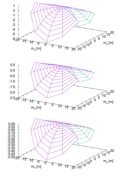
The result for prototypical E-ELT variables is shown in Figure 6: With Ciddor’s formulas for the index of refraction we assume a wavelength of 500 nm, a temperature of 10^∘ C, a pressure of 697 hPa, a CO₂ content of 470 ppm, so the refractive index is 1.000195229, and $\chi_{0}=3.9\times 10^{-4}$. The semi-major axis and flattening of the WGS84 National Imagery and Mapping Agency (2000) at a geographic latitude of $\varphi=24^{\circ}35^{\prime}$, and sea level altitude 3046 m gives a distance $\rho(0,0)=6377.5$ km to the Earth center. Results are plotted for a radius up to $\sqrt{m_{h}^{2}+m_{v}^{2}}\leq 19.6$ m and a scale height of $K=9600$ m. The conclusion is:

• There is almost no residual optical path length along the horizontal ($m_{h}$) axis (tip).

• There is essentially no tilt component left, which means a tilt of the telescope axis by $R$ as computed in Section II removes the first-order Zernike terms, as expected.

• The residual difference of the path length of the upper and lower rim ($m_{v}$) relative to the center is up to 6 $\mu$m of uni-axial defocus at a zenith distance of 60^∘.

• The residual difference is approximately proportional to the residual air mass: $|\Delta L|\propto\frac{1}{\cos z}-1$.

Figure 6: The optical path length difference $\Delta L$ in micrometer in the entrance pupil of a 40-m telescope for zenith angles of 60 (top), 40 (middle) and 20 degrees (bottom) at $\chi_{0}=3.9\times 10^{-4}$.

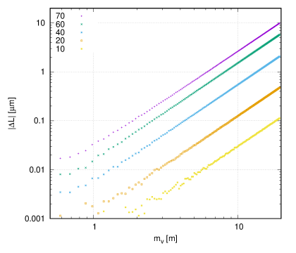
We may zoom into such a graph and plot the absolute value of $\Delta L$ in a cut from the center of the pupil to the upper rim, which yields Figure 7. This plot with a double logarithmic scale of the optical path difference shows that

• the functions are almost straight lines for zenith distances up to 60^∘; the aberration is approximately proportional to the squared distance (not a pure second-order Zernike term). For a 8m-telescope at $z=60^{\circ}$ the path difference is only 0.26 $\mu$m.

• the numerical implementation has jitters on path length scales of typically 3 nanonmeters. This is likely a consequence of rounding errors with the double-precision arithmetics in the C++ source code, plus precision limits caused by cut-offs in the number of taylor terms included while computing $\Delta L^{(1)}$ and $\Delta L^{(2)}$.

Figure 7: The absolute value of optical path length difference $\Delta L$ in microns in the entrance pupil between the upper rim and the center for zenith angles of 70, 60, 40, 20 and 10 degrees (top to bottom). These are cuts through graphs of Figure 6 at $m_{h}=0$.

In a general telescope operation effects of the order calculated here are probably not observed, because a focusing model that includes flexure compensations or wind loads as a function of zenith angle must handle basically the same data.

With another cut through the parameter set we may keep $z_{0}$ and $m_{v}$ fixed and look at $\Delta L$ as a function of the refractive index at the ground; this is relevant if the adaptive optics system and the science cameras observe at different wavelengths and hence at different $\chi_{0}$. The numerical data of Figure 8 reveal that the change in $\Delta L$ is practically proportional to $\chi_{0}$ as long as the scale height is fixed. In consequence one may map relative differential chromatic differences in the susceptibilities directly to relative differential aberrations in the entrance pupil.

Figure 8: The optical path length difference $\Delta L$ in microns in the entrance pupil at the upper rim 19.6m away from the center for a zenith angle of 60^∘.

IV Summary

In a barometric exponential model of the the air susceptibility profile above the telescope we presented approximate analytical formulas

1. of the differential zenit angle $R$ as a power series of the tangent of the zenith angle with expansion coefficients summarized in (15), (16) and (17);

2. of the path length distribution $\Delta L$ of rays in the entrance pupil with two contributions summarized by (39) and (43).

Appendix A Segregated Scale Heights

If gas mixtures of the air are treated as independent linear responses such that $\chi_{0}$ is an additive composition proportional to the weighted contribution of the air components, Equation (15) breaks already in the first three terms in the square brackets if the scale heights of the molecular constituents differ. The typical case is an additive mixture of dry air and water vapor, where dry air has a scale height $K$ near 9 kilometers, but water vapor disappears at a scale height of approximately 2 kilometers Turner et al. (2001); Cahen et al. (1982); Parameswaran and Murthy (1990); Otárola et al. (2010). To illustrate that variant, one would introduce a susceptibility with two scale heights $K_{1}$ and $K_{2}$,

$$\chi(r)=\chi_{01}e^{-(r-\rho)/K_{1}}+\chi_{02}e^{-(r-\rho)/K_{2}}=\chi_{01}e^{-(r-\rho)/K_{1}}+(1\leftrightarrow 2),$$ (44)

where $1\leftrightarrow 2$ means the previous terms is repeated where the roles of $K_{1}$ and $K_{2}$ are swapped, and also the roles of $\chi_{01}$ and $\chi_{02}$ are swapped. The lowest order expansion for small $\hat{K}_{1}\equiv K_{1}/\rho$ and $\hat{K}_{2}\equiv K_{2}/\rho$ and small $\chi_{01}$, $\chi_{02}$ is

$$\gamma_{1} = \frac{1}{2}\rho n_{0}\int_{1}^{n_{0}}\frac{1}{n^{3}r}d\chi$$ (45)

$$= \frac{1}{2}\rho n_{0}\int_{\rho}^{\infty}\frac{1}{[1+\chi_{01}e^{-(r-\rho)/K_{1}}+\chi_{02}e^{-(r-\rho)/K_{2}}]^{3/2}r}[\frac{1}{K_{1}}\chi_{01}e^{-(r-\rho)/K_{1}}+\frac{1}{K_{2}}\chi_{02}e^{-(r-\rho)/K_{2}}]dr$$

$$= \frac{1}{2}\rho n_{0}\int_{0}^{\infty}\frac{1}{[1+\chi_{01}e^{-r/K_{1}}+\chi_{02}e^{-r/K_{2}}]^{3/2}(r+\rho)}[\frac{1}{K_{1}}\chi_{01}e^{-r/K_{1}}+\frac{1}{K_{2}}\chi_{02}e^{-r/K_{2}}]dr$$

$$= \frac{1}{2}\frac{\rho}{K_{1}}n_{0}\chi_{01}\int_{0}^{\infty}\frac{e^{-r/K_{1}}}{[1+\chi_{01}e^{-r/K_{1}}+\chi_{02}e^{-r/K_{2}}]^{3/2}(r+\rho)}dr+(1\leftrightarrow 2)$$

$$\approx \frac{\chi_{01}}{8(\hat{K}_{1}+\hat{K}_{2})}\left[4(\hat{K}_{1}+\hat{K}_{2}-\hat{K}_{1}\hat{K}_{2}-\hat{K}_{1}^{2})+2\chi_{02}\hat{K}_{1}-4\chi_{02}\hat{K}_{2}-\chi_{01}(\hat{K}_{1}+\hat{K}_{2})\right]+(1\leftrightarrow 2).$$

Appendix B Cassini’s model

B.1 Tilt Correction

The Cassini model of a homogeneous single-layer atmosphere of height $h$ leads to a difference between observed and astrometric zenith angles of (Young, 2004, §9.5)Corbard et al. (2019); van den Born and Jellema (2020)

$$R^{(C)}=\arcsin\left(\frac{n_{0}\rho\sin z_{0}}{\rho+h}\right)-\arcsin\left(\frac{\rho\sin z_{0}}{\rho+h}\right).$$ (46)

The bivariate Taylor expansion in orders of $n_{0}-1$ and $q$ starts

$$R^{(C)} = (n_{0}-1)\tan z_{0}\big{[}1-\frac{q}{\cos^{2}z_{0}}+\frac{1}{2}(n_{0}-1)\tan^{2}z_{0}+\frac{1}{2}\frac{q^{2}(3-\cos^{2}z_{0})}{\cos^{4}z_{0}}-\frac{3}{2}\frac{(n_{0}-1)q\tan^{2}z_{0}}{\cos^{2}z_{0}}$$ (47)

$$\quad+\frac{1}{6}\frac{(n_{0}-1)^{2}\tan^{2}z_{0}(3-2\cos^{2}z_{0})}{\cos^{2}z_{0}}+\cdots\big{]}$$

where $q=h/\rho$. The small difference $R-R^{(C)}$ for a parameter set of $\rho=6377.36$ km, $h=K=9.6$ km and $n_{0}=1.000284$ is illustrated in Figure 9.

Figure 9: The difference between the refraction predicted by (46) and the model of exponential slope, $R-R^{(C)}$, as a function of zenith distance with $\chi_{0}=0.000568081$ and $\rho=6377.36$ km and $K=9.6$ km. Less than 30 mas for zenith angles below $70^{\circ}$.

Expansion of $R^{(C)}$ in powers of $\tan z_{0}$ defines coefficients $\gamma_{i}^{(C)}$:

$$R^{(C)}\equiv\sum_{i=1,3,5,\ldots}\gamma_{i}^{(C)}\tan^{i}z_{0},$$ (48)

such that up to third mixed order in $\chi_{0}$ and $q$

$$\gamma_{1}^{(C)}=n_{0}\chi_{0}\frac{1}{2}\left[1-\frac{3}{4}\chi_{0}-q+\frac{5}{8}\chi_{0}^{2}+\frac{3}{4}\chi_{0}q+q^{2}+\ldots\right],$$ (49)

$$\gamma_{3}^{(C)}=n_{0}\chi_{0}\frac{1}{4}\left[\frac{1}{2}\chi_{0}-2q-\frac{5}{12}\chi_{0}^{2}+5q^{2}+\ldots\right],$$ (50)

$$\gamma_{5}^{(C)}=n_{0}\chi_{0}\frac{3}{16}\left[\frac{1}{3}\chi_{0}^{2}-2\chi_{0}q+4q^{2}+\ldots\right].$$ (51)

The difference between the Cassini model and the exponential model is given by subtracting (49) and (50) from (15) and (16),

$$R-R^{(c)}\approx\frac{1}{2}n_{0}\chi_{0}\left(-\frac{3}{4}\chi_{0}q+q^{2}+\cdots\right)\tan z_{0}+\frac{1}{4}n_{0}\chi_{0}\left(-\frac{3}{2}\chi_{0}q+5q^{2}+\cdots\right)\tan^{3}z_{0}+\cdots$$ (52)

B.2 Aberration

The ray that will arrive at $(m_{h},m_{v})$ in the input pupil hits the top of the atmosphere at a global coordinate

$$[\rho(0,0)+h]\left(\begin{array}[]{c}\cos\alpha(m_{h},m_{v})\\ \sin\alpha(m_{h},m_{v})\sin\phi(m_{h},m_{v})\\ \sin\alpha(m_{h},m_{v})\cos\phi(m_{h},m_{v})\end{array}\right)$$ (53)

where $\phi$ of Eq. (21) fixes the incidence plane. The distance between this point and $\vec{m}(m_{h},m_{v})$, multiplied by $n_{0}$, is the optical path length in air (substituting $R\to R^{(C)}$ where necessary). The angle of incidence of the ray traveling above the atmosphere in the direction $(-1,0,0)$ is $\alpha$. Snell’s law gives an exit angle $\alpha^{\prime}$ of $\sin\alpha=n_{0}\sin{\alpha^{\prime}}$ relative to the local normal vector.

$$\alpha-\alpha^{\prime}=R^{(C)}=z-z_{0}.$$ (54)

The incidence point has a geometric path difference $l$ to the telescope

$$[\rho(0,0)+h]\left(\begin{array}[]{c}\cos\alpha\\ \sin\alpha\sin\phi\\ \sin\alpha\cos\phi\end{array}\right)=\rho(m_{h},m_{v})\left(\begin{array}[]{c}\cos z(m_{h},m_{v})\\ \sin z(m_{h},m_{v})\sin\phi(m_{h},m_{v})\\ \sin z\cos\phi(m_{h},m_{v})\end{array}\right)+l\left(\begin{array}[]{c}\cos R^{(C)}(m_{h},m_{v})\\ \sin R^{(C)}(m_{h},m_{v})\sin\phi(m_{h},m_{v})\\ \sin R^{(C)}(m_{h},m_{v})\cos\phi(m_{h},m_{v})\end{array}\right).$$ (55)

Adding the squares of the three Cartesian components gives a quadratic equation for $l$ which is solved by

$$l=-\rho(m_{h},m_{v})\cos z_{0}(m_{h},m_{v})+\sqrt{[\rho(0,0)+h]^{2}-\rho^{2}(m_{h},m_{v})\sin^{2}z_{0}(m_{h},m_{v})}.$$ (56)

The optical path length is this path through air plus a stretch in vacuum which we let start at a reference plane tangential to the top of the atmosphere:

$$L^{(C)}=n_{0}l+[\rho(0,0)+h](1-\cos\alpha).$$ (57)

We are only interested in path differences, so we drop the constant $\rho(0,0)+h$, then substitute the first component of the vector in Eq. (55):

$$L^{(C)} = [n_{0}-\cos R^{(C)}(m_{h},m_{v})]\left[\sqrt{[\rho(0,0)+h]^{2}-\rho^{2}(m_{h},m_{v})\sin^{2}z_{0}(m_{h},m_{v})}-\rho(m_{h},m_{v})\cos z_{0}(m_{h},m_{v})\right]$$ (58)

$$-\rho(m_{h},m_{v})\cos z(m_{h},m_{v}).$$

Insertion of (23) gives

$$\Delta L^{(C)}= [n_{0}-\cos R^{(C)}(m_{h},m_{v})]\left[\sqrt{(\rho(0,0)+h)^{2}-\rho^{2}(m_{h},m_{v})\sin^{2}z_{0}(m_{h},m_{v})}-\rho(m_{h},m_{v})\cos z_{0}(m_{h},m_{v})\right]$$

$$-[n_{0}-\cos R^{(C)}(0,0)]\left[\sqrt{(\rho(0,0)+h)^{2}-\rho^{2}(0,0)\sin^{2}z_{0}(0,0)}-\rho(0,0)\cos z_{0}(0,0)\right]+m_{v}\sin R^{(C)}(0,0)$$

$$= [n_{0}-\cos R^{(C)}(m_{h},m_{v})]\left[\sqrt{(\rho(0,0)+h)^{2}-\rho^{2}(m_{h},m_{v})\sin^{2}z_{0}(m_{h},m_{v})}-\sqrt{\rho^{2}(m_{h},m_{v})-\rho^{2}(m_{h},m_{v})\sin^{2}z_{0}(m_{h},m_{v})}\right]$$ (59)

$$-((m_{h},m_{v})\to(0,0))+m_{v}\sin R^{(C)}(0,0).$$

Numerical evaluation like in Figure 10 shows that the effect $|\Delta L^{(C)}|$ in the Cassini model is roughly a tenth of the values $|\Delta L|$ of the exponential model.

Figure 10: Absolute value of the aberrations in the pupil plane with the Cassini single-layer model, Eq. (59), with the parameters of Figure 7.

Appendix C C++ implementation

C.1 Differential zenith angle

A C++ program to compute $R$ as a function of $\chi_{0}$ and $K/\rho$ up to the order $\tan^{11}z_{0}$ with up to mixed 5th order for $\tan z_{0}$ and up to mixed 4th order for $\tan^{3}z_{0}$, $\tan^{5}z_{0}$ and higher is in the anc directory of the arXiv database. The source files are r.cxx, RefreExpo.cxx and RefrExpo.h. The program is compiled with

g++ -o r -O2 r.cxx RefrExpo.cxx

or

make

or

autoreconf -i -s
configure --prefix=$PWD
make

and is run with up to 4 options:

r [-C] [-c chi0] [-K K] [-r rho]

where chi0 is the value of $\chi_{0}$ at the telescope site, K is the scale height in meters, and rho is the sum of the Earth radius and telescope sea level altitude in meters. The switch -C produces results with Cassini’s model, using K for the layer height and rho for the earth radius. The program produces a table of $z_{0}$ in degrees and values of $R$ in arcseconds.

C.2 Input Pupil Aberration

Another C++ program to compute $\Delta L$ as a function of $\chi_{0}$, $K$, $\rho$, $m_{h}$ and $m_{v}$ is also attached. Source files are named raberr.cxx, RefreExpo.cxx, RefrExpo.h, M1aberr.cxx and M1aberr.h; it is compiled with

g++ -o raberr -O2 raberr.cxx RefrExpo.cxx M1aberr.cxx

or

make

or

autoreconf -i -s
configure --prefix=$PWD
make

and is called as

raberr [-c chi0] [-K K] [-r rho] [-R radius] [-1 Nstps] -z zenith

where chi0, K and rho have the same meaning as above, where radius is the entrance pupil (primary) radius in meters, and where zenith is the zenith angle in degrees.

If the option -1 is not used, it generates a table with three values per line suitable to create Figure 6: $m_{h}$ and $m_{v}$ in meters along concentric circles of the azimuth of the entrance pupil, and $\Delta L$ in micrometers.

If the option -1 is used, it generates a table with three values per line suitable to create Figure 7: $m_{v}$ in meters for positive $m_{v}$, $|\Delta L|$ in micrometers, and the air mass $1/\cos(z_{0})$. Nstps is the number of points on the $m_{v}$ axis with a maximum set by radius.

The Maple program CassAber.mp computes a table of values like shown in Figure 10. Because this is a straight implementation without any further precautions against cancellations of digits, the internal number of digits has been set to near-quad precision in the program. The procedure Cassgam contains an extended version of the $\gamma_{i}^{(C)}$-expansions following (49).